Algorithm/Architecture Co-design of Proportionate-type LMS Adaptive Filters for Sparse System Identification

Abstract

This paper investigates the problem of implementing proportionate-type LMS family of algorithms in hardware for sparse adaptive filtering applications especially the network echo cancelation. We derive a re-formulated proportionate type algorithm through algorithm-architecture co-design methodology that can be pipelined and has an efficient architecture for hardware implementation. We study the convergence, steady state and tracking performances of these re-formulated algorithms for white, color and speech inputs before implementing them in hardware. To the best of our knowledge this is the first attempt to implement proportionate-type algorithms in hardware. We show that Delayed $\mu$-law Proportionate LMS (DMPLMS) algorithm for white input and Delayed Wavelet MPLMS (DWMPLMS) for colored input are the robust VLSI solutions for network echo cancelation where the sparsity of the echo paths can vary with time. We implemented all the designs considering $16$-bit fixed point representation in hardware, synthesized the designs and synthesis results show that DMPLMS algorithm with $\approx 25\%$ increase in hardware over conventional DLMS architecture, achieves $3X$ improvement in convergence rate for white input and DWMPLMS algorithm with $\approx 58\%$ increase in hardware achieves $15X$ improvement in convergence rate for correlated input conditions.

I Introduction

Many real-life systems such as network echo cancelation [1], underwater communication [2] and HDTV terrestrial transmission [3] exhibit impulse responses which are often sparse and sparse system identification [4] became an important research area in the last decade with the invention of proportionate-type algorithms. First member of Proportionate-type LMS family of algorithms is the Proportionate Normalized Least Mean Square (PNLMS) algorithm [5], which updates the filter coefficients by assigning a gain proportional to the magnitude of the current coefficient. The PNLMS algorithm has been shown to outperform the LMS and NLMS [6] algorithms when operating on a sparse impulse response.

However, PNLMS algorithm performance degrades and becomes worse than the NLMS algorithm when the impulse response is dispersive. Several improved PNLMS algorithms [7]- [9] were proposed in literature to address this issue and to make the algorithms more robust against varying sparsity.

Another set of algorithms was designed by seeking a condition to achieve the fastest overall convergence when all coefficients reach the $\epsilon$-vicinity of their true values simultaneously (where $\epsilon$ is a small positive number). This approach results in the $\mu$-law PNLMS (MPNLMS) [10] and its variant $\epsilon$-law PNLMS [11] (EPNLMS). The MPNLMS algorithm addresses the issue of assigning too much update gain to large coefficients, which occurs in the PNLMS algorithms. Even the MPNLMS convergence rate becomes prohibitively slow for correlated input conditions such as speech. Wavelet MPNLMS (WMPNLMS) [12] is designed to address this issue by de-correlating the input at the same time preserving the sparseness of the impulse response.

As we can see significant research effort has been dedicated to the development of high-performance adaptive algorithms based on proportionate adaptation. However, much less is known about their optimized implementation in dedicated hardware because of the huge computational penalty. In this paper we try to address this gap. To the best of our knowledge this is the first attempt to implement proportionate type algorithms in hardware. we make several reformulations to the original PNLMS algorithm to make it VLSI friendly and the reformulated algorithm is implemented in hardware. Our main contributions include :

1. Various proportionate-type LMS algorithms and their VLSI implementation aspects are studied in detail.

2. Proposed DMPLMS for white input and DWMPLMS algorithm for color input through algorithm-architecture co-design and we show that the entailed loss in performance due to complexity reduction is negligible.

3. Proposed a novel multiplier-less $3$-level sliding HAAR wavelet transform for DWMPLMS algorithm, to exploit the redundancies that exist in wavelet computation of streaming input samples .

4. As a proof-of-concept, we provide a synthesis study in $180$nm-CMOS technology of the proposed DPLMS, DMPLMS and DWMPLMS architectures and compare the improvement in rate of convergence vs hardware efficiency.

The rest of the paper is organized as follows. In the next section, we explain the motivation and formulate the problem. In Section III, we propose the algorithmic re-formulations and the corresponding VLSI architecture. Section IV deals with the transform domain proportionate type algorithms and their VLSI implementation aspects. Simulation results are presented in Section V and ASIC synthesis results are presented in Section VI and we conclude the paper in Section VII.

II Background and Motivation

II-A Review of Proportionate-type NLMS (Pt-NLMS) Algorithms

Consider the problem of identifying an unknown sparse system modeled by the $L$ tap coefficient vector $\textbf{w}_{opt}$ which takes a signal $u(n)$ with variance $\sigma_{u}^{2}$ as input and produces the observable output $d(n)=\textbf{w}_{opt}^{T}\textbf{u}(n)+v(n)$, where $\textbf{u}(n)=[u(n),u(n-1),...,u(n-L+1)]^{T}$ is the input regressor and $v(n)$ is an observation noise with variance $\sigma_{v}^{2}$ which is assumed to be white and independent of $u(m)$, for all m, n. Then the Pt-NLMS algorithm iteratively updates the filter coefficient vector, $\textbf{w}=[w_{0},w_{1},...,w_{L-1}]^{T}$ as follows:

$$\textbf{w}(n+1)=\textbf{w}(n)+\mu\frac{\textbf{G}(n)\textbf{u}(n)e(n)}{\textbf{u}^{T}(n)\textbf{G}(n)\textbf{u}(n)+\delta_{p}},$$ (1)

where the estimated error $e(n)=d(n)-y(n)$ with filter output $y(n)=\textbf{w}^{T}(n)\textbf{u}(n)$ and $\mu$ is the adaptation step size. $\delta_{p}$ is the regularization parameter, and $\textbf{G}(n)$ is the gain matrix. This gain matrix is the key factor here which distinguishes Pt-NLMS from conventional NLMS. The gain matrix $\textbf{G}(n)$ is diagonal i.e., $\textbf{G}(n)=diag(g_{0}(n),g_{1}(n),...g_{L-1}(n))$, with $g_{i}(n)\propto|w_{i}(n)|$ is the gain factor for the tap $i$. For Proportionate NLMS, $g_{i}(n)$ is evaluated as follows:

$$g_{i}(n)=\frac{\gamma_{i}(n)}{\frac{1}{L}\sum\limits_{i=0}^{L-1}\gamma_{i}(n)},\mspace{8.0mu}0\leq i\leq(L-1),$$ (2)

where

$$\gamma_{i}(n)=max[\rho\mspace{4.0mu}\gamma_{min}(n),\mathrm{F}[|w_{i}(n)|]]$$ (3)

$$\gamma_{min}(n)=max(\delta,\mathrm{F}[|w_{0}(n)|],...,\mathrm{F}[|w_{L-1}(n)|],$$ (4)

$\mathrm{F}[|w_{i}(n)|]=|w_{i}(n)|$ for PNLMS. here $\delta$ is used to prevent the coefficients from stalling during initialization stage when all the coefficients are reset to $0$. The parameter $\rho$ ensures minimum gain to inactive coefficients. It can be seen that if the current magnitude of a coefficient is large, a large step size parameter will be assigned, where as for a small coefficient the proportionate step size is small. In this way it emphasizes the large coefficients to speed up their convergence, so it demonstrates very fast initial convergence for sparse impulse response. However, this performance improvement comes at the cost of complexity. In their $2004$ Freescale application note [13] Dybe et.al. felt that because of a significant computational penalty imposed by the modified adaptation formula combined with the generation of matrix $G(n)$, the PNLMS algorithm appears to be most suitable for implementation in an ASIC technology. However, Jie, Chen in his PhD dissertation in $2008$ [14] stated that ’The high complexity associated with both PNLMS and IPNLMS algorithms makes them unsuitable for hardware implementation’. In the light of these two observations, we carry out a detailed complexity analysis of the PNLMS algorithm to show its inapplicability for VLSI implementation in its native form.

II-B Complexity Analysis

There are four main tasks performed in each iteration of the PNLMS which are elaborated below and all these steps need to be completed for one iteration before proceeding to the next iteration.

1. Filter output calculation: This step is basically computing the inner product of input vector with the weight vector which requires L multiplications which can happen in parallel and adding all the partial results in an adder tree structure which require L adders and has a time complexity of $T_{mult}+\log_{2}(L)T_{add}$.

2. Weighted euclidian norm calculation : This step is to calculate the vector matrix vector product $\textbf{u}^{T}(n)\textbf{G}(n)\textbf{u}(n)+\delta_{p}$ in each iteration which requires $2$L multiplications, L additions and has time complexity of $2T_{mult}+(1+log_{2}(L))T_{add}$

3. Gain Calculation : This has two max finding steps, one multiplication, one division, one $F(.)$ evaluation and summation of L terms and has time complexity of $2log_{2}(L)T_{cmp}+T_{mult}+T_{div}+T_{F_{eval}}$.

4. Weight update : This requires L multiplications and L additions and all of them can happen in parallel. Thus time complexity is $T_{mult}+T_{add}$.

The complexities of all the steps are summarized in Table 1 and Table 2. We see that time complexities of all the steps add up for the critical path which is shown below:

$$T_{crit}=5T_{mult}+(2+3log_{2}(L))T_{add}+2log_{2}(L)T_{cmp}+T_{div}+T_{F\_eval}.$$

This severely limits the applicability of the original PNLMS algorithm for real-time VLSI implementations which have stringent throughput requirements. In order to achieve an efficient VLSI implementation, actions must be taken at the algorithm level to further simplify the complexity characteristic of PNLMS (without compromising the performance) before going into the architecture design. We discuss these simplifications in the next section.

Table I: Area Complexity of PNLMS

  Step Mult Div Add Cmp   Filter output L 0 L 0 Weighted normalization 2L 0 L 0 Weight update 2L 1 L 0 Gain calculation 2 1 L 2L  

Table II: Time Complexity of PNLMS

Step	Critical path
Filter output	$T_{mult}+\log_{2}(L)$
Weighted normalization	$2T_{mult}+(1+log_{2}(L))T_{add}$
Weight update	$T_{mult}+T_{add}$
Gain calculation	$2log_{2}(L)T_{cmp}+T_{mult}+T_{div}+T_{F_{eval}}$

III Algorithmic Re-formulations and proposed architecture

In this section we make several reformulations to the original PNLMS algorithm to make it VLSI friendly without compromising the performance of the algorithm. To ensure this, we compare the performance of the algorithm after each simplification with that of the original algorithm and finally we design a low complexity VLSI architecture for the re-formulated algorithm.

III-A Simplified Gain Calculation

The first simplification is in the calculation of the gain calculation. For the simplified PNLMS algorithm, the gain factors are evaluated as follows:

$$g_{i}(n)=\frac{\gamma_{i}(n)}{\sum\limits_{i=0}^{L-1}\gamma_{i}(n)},\mspace{8.0mu}0\leq i\leq(L-1),$$ (5)

where

$$\gamma_{i}(n)=\mathrm{F}[(w_{i}(n)+\rho)],$$ (6)

and

$$\mathrm{F}[(w_{i}(n)=|w_{i}(n)|.$$ (7)

the parameter $\rho$ is a small positive constant added to avoid the stalling when all the tap weights are zero at the reset and also to ensure minimum gain to the inactive coefficients. We can see that even with this simplified gain calculation, the adaptation gain is proportional to the magnitude of the filter tap at time index $n$. The simplified gain calculation avoids the usage of the $max$ functions which are employed in the original PNLMS, there by reduces the time complexity. We can use an adder tree structure for adding the absolute weights of all the taps to get the denominator of Eq. 5 and then the reciprocal of this sum can be fed to all the taps for proportional gain calculation.

III-B Proportionate LMS

Unlike the NLMS, the normalization in the denominator of PNLMS update is a weighted normalization of the input vector and the weight matrix (G) changes in each iteration. So we can’t compute the normalization term recursively and calculating this vector matrix vector product freshly in each iteration requires 2L multiplications, L additions and adds significant area and time complexity (complexity grows with L, L would be generally large for real-time applications) to the already complex proportionate adaptation. To alleviate this problem, we proposed PLMS [15] (which is similar to LMS) by removing this weighted normalization and analyzed the convergence performance and it is shown that the PLMS algorithm is stable under $0<\mu<2$ for a white input with mean zero and unit variance and is able to perform as the original PNLMS. The PLMS update equation is given by,

$$\textbf{w}(n+1)=\textbf{w}(n)+\mu\hskip 1.42262pt{\textbf{G}}(n)\hskip 1.42262pt\textbf{u}(n)\hskip 1.42262pte(n),$$ (8)

where gain matrix calculation is same as that of simplified PNLMS algorithm. Now, the performance of the re-formulated algorithm is compared (with simplified gain calculation and without normalization) with that of the original PNLMS. For this, we considered a sparse system identification problem and we use the the sparseness measure $S_{m}=\frac{L}{L-\sqrt{L}}\big{(}1-\frac{{\parallel h\parallel}_{1}}{\sqrt{L}{\parallel h\parallel}_{2}}\big{)}$ to characterize the sparse system. The unknown system of length $512$ of which only $64$ taps are active ($S_{m}=0.8637$) is considered. Learning curves (Normalized MSD vs Iterations) shown in Fig. 1 are obtained by averaging over $500$ experiments. All the other simulation parameters are shown in the text box. As we can see PNLMS and reformulated PLMS outperforms the conventional NLMS significantly. We can also see that the performances of reformulated PLMS and PNLMS are same and there is no penalty for the proposed reformulations.

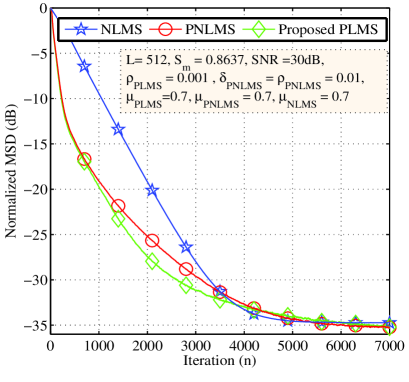
Fig. 1: Performance comparison of PNLMS with Reformulated PLMS

III-C Delayed Proportionate LMS (DPLMS)

The LMS algorithm in its original form is not suitable for realtime VLSI implementations because of the coefficient update feedback loop. To overcome this, LMS is modified to a form known as delayed LMS (DLMS) [16]-[17] with an assumption that the error gradient $e(n)*{\bf u}(n)$ does not change much with the delay $M$. The weight update equation of DLMS is shown below:

$$\begin{split}{\bf w}(n+1)={\bf w}(n)+\mu\hskip 1.42262pt{\bf u}(n-M)\hskip 1.42262pte(n-M),\end{split}$$ (9)

where $e(n-M)=d(n-M)-y(n-M)$. With the introduction of the $M$ delay registers in the feedback loop, we can apply re-timing [18] to the LMS circuit, so that the critical path is reduced to either one multiplier $T_{mult}$ or one adder $T_{add}$ as desired by the application. The concept of delayed adaptation can be extended to proportionate LMS also and the corresponding weight update equation for the delayed PLMS (DPLMS) algorithm is given by,

$$\textbf{w}(n+1)=\textbf{w}(n)+\mu{\textbf{G}(n-M)\textbf{u}(n-M)e(n-M)},$$ (10)

where

$$\textbf{G}(n-M)=diag(g_{0}(n-M),g_{1}(n-M),...g_{L-1}(n-M)),$$ (11)

with

$$g_{i}(n-M)=\frac{\gamma_{i}(n-M)}{\sum\limits_{i=0}^{L-1}\gamma_{i}(n-M)},\mspace{8.0mu}0\leq i\leq(L-1),$$ (12)

and

$$\gamma_{i}(n-M)=\mathrm{F}[(w_{i}(n-M)+\rho)],$$ (13)

$$\mathrm{F}[(w_{i}(n-M)=|w_{i}(n-M)|.$$ (14)

Now we compare the performance of the DPLMS with that of PLMS. We consider the same sparse system identification problem as in last subsection and simulation parameters are shown in the text box. Learning curves (Normalized MSD vs Iterations) shown in Fig. 2 are obtained by averaging over $500$ experiments. We can notice that after the initial phase, the convergence rate of the PLMS algorithm slows down significantly, even becoming slower than NLMS. The large coefficients converge very fast at the cost of slowing down dramatically convergence of the small coefficients. DPLMS suffers even more because of the direct proportional gain and delayed adaptation. To address this issue, these re-formulations are extended to the $\mu$-Law PLMS (MPLMS) which has more balanced gain distribution.

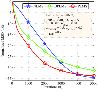
Fig. 2: Performance comparison of PLMS with Delayed PLMS

III-D Delayed $\mu$-Law PLMS (DMPLMS)

$\mu$-Law PNLMS (MPNLMS) [10] offers more balanced distribution of the adaptation energy among all the coefficients as it is based on the optimization criteria that all the coefficients converge simultaneously to the $\epsilon$-vicinity of their true value so that the overall convergence is the fastest. Here gain is proportional to the natural logarithm of the absolute value of the current weight instead of the absolute of current weight itself. This logarithm in the $\mathrm{F}[(.)]$ equation (which is shown below) is the only difference between MPNLMS and PNLMS. The parameter $\xi$ is a very small positive number and its value should be chosen based on the measurement noise level. For applications such as network echo cancelation, $\xi=0.001$ is a good choice because the echo below $-60dBm$ is negligible.

$$\mathrm{F}[(w_{0}(n))]=\ln(1+\frac{|w_{0}(n)|}{\xi}).$$ (15)

We extended all the aforementioned re-formulations to MPNLMS and also we simplified the $\mathrm{F}[(.)]$ equation to the following equation for our VLSI implementations and verified its effectiveness through simulations. Since we changed the natural logarithm to base-2 logarithm, $k$ is chosen to be $6$.

$$\mathrm{F}[(w_{0}(n))]=\log_{2}(1+\frac{|w_{0}(n)|}{2^{-k}}).$$ (16)

Because of this balanced gain distribution delayed adaptation of MPLMS doesn’t suffer much and performances of MPLMS and DMPLMS (for same experimental conditions) are shown in Fig. 3. We can see that delayed MPLMS with logarithmic simplifications is a robust algorithm for white input case which is suitable for VLSI implementation. The formal algorithm is summarized in Algorithm 1.

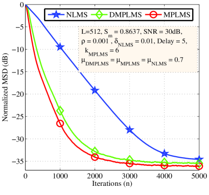
Fig. 3: Performance comparison of MPLMS with Delayed MPLMS

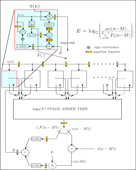
Fig. 4: MPLMS Architecture

Initialization : $w_{i}(1)=0,\mspace{8.0mu}0\leq i\leq(L-1)$

Parameters : $\mu$, $\rho$, $k$

Updation :

$e(n)=d(n)-\textbf{w}^{T}(n)\textbf{u}(n)$

$\mathrm{F}[(w_{i}(n))]=\log_{2}(1+\frac{|w_{i}(n)|}{2^{-k}})$

$\gamma_{i}(n)=\mathrm{F}[(w_{i}(n)+\rho)]$

$g_{i}(n)=\frac{\gamma_{i}(n)}{\sum\limits_{i=0}^{L-1}\gamma_{i}(n)},\mspace{8.0mu}0\leq i\leq(L-1)$

$\textbf{G}(n)$ = $diag(g_{0}(n),g_{1}(n),...g_{L-1}(n))$

$\Delta\textbf{W}=\mu{\textbf{G}(n-M)\textbf{u}(n-M)e(n-M)}$

$\textbf{w}(n+1)=\textbf{w}(n)+\Delta\textbf{W}$

Algorithm 1 Delayed MPLMS algorithm

III-E Logarithmic Number System to calculate the gradient

Even the simplified DPLMS gradient calculation involves division and fixed point division is quite a bit more complicated [19] than fixed point multiplication, and usually takes a lot more cycles than performing a multiplication. Thus we use logarithmic number system (LNS) which simplifies the division. The logarithmic conversion of a real number $Q$ can be obtained by $\log_{2}(Q)=k+\log_{2}(1+x)$ when $Q=2^{k}(1+x)$, $k$ is the leading one bit position and $x$ is a fraction. Depending on how we approximate this $\log_{2}(1+x)$ there have been multiple schemes in the literature. This can be achieved by using a LUT with $x$ as index and $\log_{2}(1+x)$ as the value or performing simple conversion on $x$. Mitchell [20] used the value of $x$ to directly approximate $\log_{2}(1+x)$. In this scheme the log-converter contains a simple Leading One Detector (LOD) circuit followed by a barrel shifter and antilog converter is a concatenation of $1$ and $x$ followed by a barrel shifter. DMPLMS architecture employing these log/antilog converters will be explained in the next section.

III-F Proposed Architecture

The architecture for the proposed DMPLMS and DPLMS is shown in Fig. 4. Please note that the only difference between DPLMS and DMPLMS architectures is the $F(.)$ module. One of the PLMS/MPLMS tap is zoomed and showed separately. Each tap gets two inputs one is the regressor input from the tapped delay line, the other is the quantity E, which is defined as,

$$E=\log_{2}\left(\frac{\mu\hskip 1.42262pte(n-M)}{\sum\limits_{i=0}^{L-1}F_{i}(n-M)}\right).$$ (17)

and it is used in the gradient calculation. As mentioned in previous subsection, to reduce the complexity we use the LNS for gradient calculation. Since logarithm of a negative number is undefined, we take the logarithm of absolute value of $e(n-M)$ and propagate the sign of $e(n-M)$ to the sign conversion unit in each tap. Please note that sign of this E is same as sign of $e(n-M)$ as the denominator of Equation (17) is always positive. Gradient in LNS format can be written as

$$\Delta\textbf{W}=2^{\log_{2}(\mu\hskip 1.42262pt{\textbf{G}}(n-M)\hskip 1.42262pt\textbf{u}(n-M)\hskip 1.42262pte(n-M))}.$$ (18)

By expanding the gain matrix and by separating the terms which are independent of tap and which are dependent on tap, we get

$$\Delta\textbf{W}=2^{\log_{2}\left(\frac{\mu\hskip 1.42262pt|e(n-M)|}{\sum\limits_{i=0}^{L-1}\mathrm{F}[w_{i}(n-M)]}\right)+\log_{2}({\mathrm{F}[|w_{i}(n-M)|]|\textbf{u}(n-M)})|}.$$ (19)

By replacing the first term with E which was defined above, we get the final equation for the gradient

$$\Delta\textbf{W}=2^{E+\log_{2}(\mathrm{F}[w_{i}(n-M)])+\log_{2}(|\textbf{u}(n-M)|)}.$$ (20)

As shown in each tap, logarithms of $\mathrm{F}[|w_{i}(n)|])$ and $|u_{i}(n)|$ are added and delayed by the required amount to match the delay in the filter output path and the sum is then added to $E$, finally antilogarithm is applied to the resultant to get the magnitude of the gradient. Sign of the gradient is decided by XOR operation between sign$(e(n-M))$ and sign$(u(n-M))$. After the required sign conversion, the result is added to the old weight to get the new weight for each tap. Each tap generates two outputs namely $Tap\_out$ and $\mathrm{F}[w_{i}(n)]$. These two quantities of all the taps need to be added using an adder tree structure to calculate the final filter output and the denominator of the gain matrix respectively. So we fold the adder tree by a folding factor of $2$ i.e., use the same adder tree in a time shared fashion to calculate both these quantities. If we use a carry save adder tree, the propagation delay would be less and thus we can run the adder tree at twice the clock rate compared to the FIR filter.

III-G Fixed point implementation

We have done simulations using MATLAB with $16$-bit fixed point representations and with all the above suggested re-formulations and compared the results with those of floating point simulations to see if the algorithms are tolerant to the re-formulations and LNS approximations. Fig. 5 shows the comparison of both DPLMS and DMPLMS algorithms learning curves of MSD by averaging over $10$ runs. Because of the iterative and stochastic nature of the algorithms, we can notice that they are tolerant to the logarithmic approximations and hence $16$-bit fixed point and floating point curves coincide.

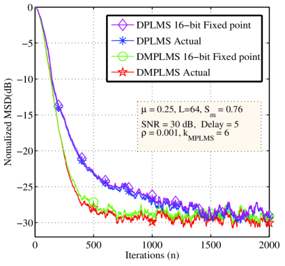
Fig. 5: Performance of fixed point implementation

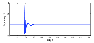
(a) Sparse Impulse Response.

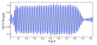
(b) DCT Weights.

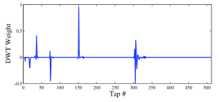
(c) DWT Weights.

Fig. 6: Comparison of DCT/DWT coefficients.

IV Transform Domain Delayed Wavelet MPLMS Algorithm

IV-A Motivation

The convergence performance of LMS-type filters is highly dependent on the correlation of the input data and, in particular, on the eigenvalue spread of the input correlation matrix $\bf{R}$. Because of this, the convergence of LMS-type filters becomes prohibitively slow for correlated input such as speech. We also found that the effect of delayed adaptation on the convergence is much more pronounced in the case of colored input compared to the white input, which can be observed from Fig. 7,

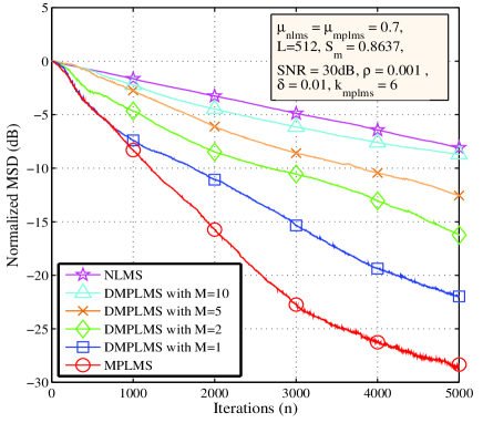
Fig. 7: Performance degradation of DMPLMS for color input

It can also be noted that the performance degrades with the adaptation delay $M$ for the DMPLMS algorithm and becomes worse than that of NLMS when the adaptation delay is increased beyond $10$ clocks. This problem can be addressed by transform domain adaptive filters [21]. The main idea behind transform domain adaptive filters is that a de-correlating unitary transform is applied to the input and then by power normalizing each input component in the transform domain, we can make the autocorrelation matrix approximately an identity matrix. This approximate white input is then fed to the adaptive filter for adaptation. However, please note that now the estimated filter weights are also in transform domain. Hence we need to select the transform which de-correlates the input while preserving the sparsity of the transformed filter weights. For example Discrete Cosine Transform (DCT) [21] which has excellent de-correlating properties but doesn’t preserve the sparsity which can be observed from Fig. 6(a) and Fig. 6(b), and thus we will loose the advantage of proportional adaptation. On the other hand, Discrete Wavelet Transform (DWT) with its time frequency localization property, preserves the sparseness of impulse response [22] as shown in Fig.6(c) and also exhibits decent de-correlation property. Thus Wavelet MPNLMS (WMPNLMS) [12] is more suitable for sparse adaptive filters under correlated input. Hence, before feeding the input to the proposed DMPLMS adaptive filter, it will be de-correlated using DWT. The resultant DWMPLMS algorithm with all the proposed re-formulations is summarized in Algorithm 2.

Initialization : $w_{i}(1)=0,\mspace{8.0mu}0\leq i\leq(L-1)$

Parameters : $\mu$, $\rho$, $\beta$, $k$

Updation :

$\textbf{u}_{T}(n)=\textbf{T}\textbf{u}(n)$

$\Psi_{i}(n)=\beta\Psi_{i}(n-1)+(1-\beta)|(u_{T,i}(n))|,\mspace{8.0mu}0\leq i\leq(L-1)$

$\textbf{D}(n)$ = diag($\Psi_{i}(n)$)

$e(n)=d(n)-\textbf{w}_{T}^{T}(n)\textbf{u}_{T}(n)$

$\mathrm{F}[(w_{T,i}(n))]=\log_{2}(1+\frac{|w_{T,i}(n)|}{2^{-k}})$

$\gamma_{i}(n)=\mathrm{F}[(w_{T,i}(n))+\rho]$

$g_{i}(n)=\frac{\gamma_{i}(n)}{\sum\limits_{i=0}^{L-1}\gamma_{i}(n)},\mspace{8.0mu}0\leq i\leq(L-1)$

$\textbf{G}(n)$ = $diag(g_{0}(n),g_{1}(n),...g_{L-1}(n))$

$\Delta\textbf{w}=\mu{\textbf{G}(n-M)\textbf{D}^{-1}(n-M)\textbf{u}(n-M)e(n-M)}$

$\textbf{w}_{T}(n+1)=\textbf{w}_{T}(n)+\Delta\textbf{w}$

Algorithm 2 Delayed WMPLMS algorithm

In the next section we study different wavelet transforms and their convergence performances in the framework of delayed proportionate adaptation.

IV-B Study of various wavelet Transforms and their de-correlating properties

We considered three families of wavelets [23] namely Haar, Symlets denoted as Sym4 and Daubechies denoted as db4 for the comparative study of their convergence performance when used in DWMPLMS algorithm and the results are shown in Fig. 8. We see that DWMPLMS algorithms outperforms DMPLMS and DPLMS algorithms significantly. Among the wavelet families Sym4 perform better than the other two. Even though Haar wavelet’s performance is inferior to the other two, when we consider the performance complexity tradeoff as a metric, we show that Haar is the better than the rest. Next we analyzed the performance with various levels of Haar decomposition and we noticed that there is a significant performance improvement from two to three levels and beyond three levels of decomposition the performance improvement is negligible. Thus we considered $3$-level Haar wavelet for implementing DWMPLMS algorithm. In the next section we show that how a fast sliding wavelet transform can be computed by taking the streaming nature of the input data into account.

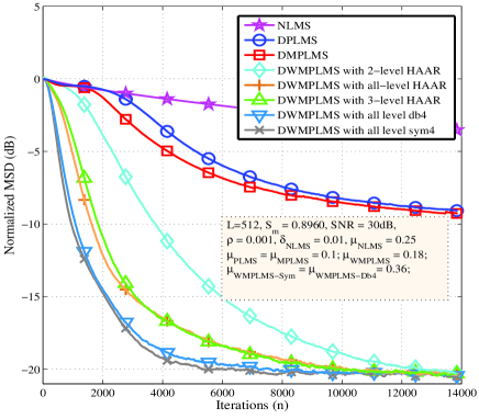
Fig. 8: Performance of 3-level HAAR DWMPLMS

IV-C Sliding Wavelet transform

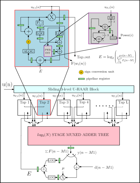
(a) DWMPLMS Architecture.

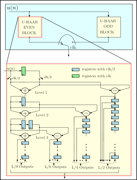
(b) Sliding HAAR Architecture.

Fig. 9: Proposed Architectures.

The data vector $\textbf{u}(n)$ (which is defined as $\textbf{u}(n)=[u(n)u(n-1)...u(n-N+1)]^{T}$) is updated at each new iteration by letting one data sample to enter in and one to leave. The transformed input vector is denoted by $\textbf{u}_{T}(n)$ i.e. $\textbf{u}_{T}(n)=\textbf{T}\textbf{u}(n)$. The streaming nature of the input can be used to exploit the redundancies that exist between calculation of running wavelet transforms of $\textbf{u}(n)$ and $\textbf{u}(n+2)$ (where $\textbf{u}(n+2)=[u(n+2)u(n+1)...u(n-N+3)]^{T}$). Let $\textbf{T}_{8}$ be 8-point $Sym2$ DWT which has four low frequency coefficients $h0,h1,h2$ and $h3$ and four high frequency coefficients $g0,g1,g2$ and $g3$. Now consider the matrix vector products $\textbf{T}_{8}\textbf{u}(n)$ which is shown below and $\textbf{T}_{8}\textbf{u}(n+2)$ for an $8$-tap filter

$$\begin{pmatrix}h0&h1&h2&h3&0&0&0&0\\ 0&0&h0&h1&h2&h3&0&0\\ 0&0&0&0&h0&h1&h2&h3\\ h2&h3&0&0&0&0&h0&h1\\ g0&g1&g2&g3&0&0&0&0\\ 0&0&g0&g1&g2&g3&0&0\\ 0&0&0&0&g01&g1&g2&g3\\ g2&g3&0&0&0&0&g0&g1\end{pmatrix}\begin{pmatrix}u(n)\\ u(n-1)\\ u(n-2)\\ u(n-3)\\ u(n-4)\\ u(n-5)\\ u(n-6)\\ u(n-7)\end{pmatrix}.$$

In [24], it has been shown that by defining basic adder cells and reusing the partial sums, computational complexity can be significantly reduced and the number of multiplications can even become independent of the filter order under certain conditions. However, this reduction is true only for one level of decomposition. Once we go for second level of decomposition, i.e., $\left(\begin{matrix}\textbf{T}_{4}&\textbf{0}_{4}\\ \textbf{0}_{4}&\textbf{I}_{4}\end{matrix}\right)\textbf{T}_{8}\textbf{u}(n)$, the redundancies cease to exist since the wavelet coefficients obtained in the first level, i.e., $\textbf{T}_{8}\textbf{u}(n)$ no longer have the streaming nature.

This complicates the wavelet transform computation and thus not suitable for DWMPLMS algorithm where we need at least 3-levels of decomposition to get good de-correlating properties. On the other hand if we consider the un-normalized Haar wavelet whose coefficients are simple $\pm 1$s, the redundancies continue to exist through multiple levels of decomposition and we can exploit them using a regular structure. For example consider 8-point un-normalized HAAR wavelet matrix with two levels of decomposition (i.e., the product matrix $\begin{pmatrix}\textbf{T}_{4}&\textbf{0}_{4}\\ \textbf{0}_{4}&\textbf{I}_{4}\end{pmatrix}\textbf{T}_{8}$ ) which is shown below:

$$\begin{pmatrix}1&1&1&1&0&0&0&0\\ 0&0&0&0&1&1&1&1\\ 1&1&-1&-1&0&0&0&0\\ 0&0&0&0&1&1&-1&-1\\ 1&-1&0&0&0&0&0&0\\ 0&0&1&-1&0&0&0&0\\ 0&0&0&0&1&-1&0&0\\ 0&0&0&0&0&0&1&-1\end{pmatrix}\begin{pmatrix}u(n)\\ u(n-1)\\ u(n-2)\\ u(n-3)\\ u(n-4)\\ u(n-5)\\ u(n-6)\\ u(n-7)\end{pmatrix}.$$

Now, consider the low frequency wavelet components at $n^{th}$ time index

$$\begin{split}u_{T,0}(n)&=u(n)+u(n-1)+u(n-2)+u(n-3),\\ u_{T,1}(n)&=u(n-4)+u(n-5)+u(n-6)+u(n-7),\\ u_{T,2}(n)&=u(n)+u(n-1)-[u(n-2)+u(n-3)],\\ u_{T,3}(n)&=u(n-4)+u(n-5)-[u(n-6)+u(n-7)],\\ \end{split}$$ (21)

if we define $a(n)=u(n)+u(n-1)$, then $u_{T,0}(n)=a(n)+a(n-2)$ and $u_{T,2}(n)=a(n)-a(n-2)$. Similarly at $(n+2)^{th}$ time index

$$\begin{split}u_{T,0}(n+2)&=u(n+2)+u(n+1)+u(n)+u(n-1),\\ u_{T,1}(n+2)&=u(n-2)+u(n-3)+u(n-4)+u(n-5),\\ u_{T,2}(n+2)&=u(n+2)+u(n+1)-[u(n)+u(n-1)],\\ u_{T,3}(n+2)&=u(n-2)+u(n-3)-[u(n-4)+u(n-5)].\\ \end{split}$$ (22)

Now, $u_{T,0}(n+2)=a(n+2)+a(n)$ and $u_{T,2}(n+2)=a(n+2)-a(n)$. Note that only $a(n+2)$ need to be evaluated at $(n+2)^{th}$ time index and all the other partial sums can be reused. Similarly high frequency components at $n^{th}$ time index

$$\begin{split}u_{T,4}(n)&=u(n)-u(n-1),\\ u_{T,5}(n)&=u(n-2)-u(n-3),\\ u_{T,6}(n)&=u(n-4)-u(n-5),\\ u_{T,7}(n)&=u(n-6)-u(n-7),\\ \end{split}$$ (23)

and at $(n+2)^{th}$ time index

$$\begin{split}u_{T,0}(n+2)&=u(n+2)-u(n+1),\\ u_{T,0}(n+2)&=u(n)-u(n-1),\\ u_{T,0}(n+2)&=u(n-2)-u(n-3,\\ u_{T,0}(n+2)&=u(n-4)-u(n-5).\\ \end{split}$$ (24)

Once two input samples are subtracted, the resultant is passed through a tapped delay line and $\frac{L}{2}$ outputs are taken from $\frac{L}{2}$ registers. Similar redundancies exist between $(n-1)^{th}$ and $(n+1)^{th}$ time indices. This scheme can be extended to multiple levels of decomposition using only adders/subtractors and registers. However, please note that un-normalized Haar wavelet is non-orthogonal and this creates issue while computing the filter output, which need to be addressed and it is explained later. The architecture of DWMPLMS with sliding wavelet implementation is explained in the next section.

IV-D Proposed Architecture

DWMPLMS architecture is shown in Fig. 9(a) and is similar to DMPLMS Architecture except for the sliding wavelet transform block, muxed adder tree and power normalization block in each tap. These changes will be explained in detail. In this subsection we explain the sliding Haar wavelet block and in subsequent sections we explain the others. Sliding un-normalized Haar wavelet implementation is shown in the Fig. 9(b). It contains two identical blocks U-HAAR even and U-HAAR odd blocks. U-HAAR even block is zoomed and shown separately. The switches shown in this U-HAAR even block closes at the rate of $\frac{clk}{2}$ so as to sample only non-overlapped even pairs like $u(n),u(n-1)$ and $u(n+2),u(n+1)$. Similarly the odd pairs $u(n+1),u(n)$ and $u(n+3),u(n+2)$ are sampled in U-HAAR odd block. Once the even pair is received, it is added and subtracted to get the low and high frequency components and high frequency components are passed through a series of registers which are clocked on $\frac{clk}{2}$ which forms the tapped delay line and the $\frac{L}{2}$ high frequency outputs come from this delay line. The low frequency components are passed through the second level of decomposition. For second level difference components, valid outputs are generated once in four clocks. Hence we require two registers which run on $\frac{clk}{2}$. If we use one register which run on $\frac{clk}{4}$, we loose the intermediate results and hence output would be erroneous. Except the top latch shown in green color, all other latches run on $\frac{clk}{2}$. Similarly in the third level, we need four registers running on $\frac{clk}{2}$ between valid outputs to capture all the intermediate results. In the first level, we need $\frac{(L-2)}{2}$ registers for the difference. Similarly at the second stage we need $\frac{(L-4)}{2}$ registers and at the final stage we need $\frac{(L-8)}{2}$ registers for detail coefficients and another $\frac{(L-8)}{2}$ registers for average coefficients. We see that it is a register hungry design but the critical path is just three adders/subtractors since there are no multipliers. Similarly the redundancies between $\bf{u}(n+1)$ and $\bf{u}(n-1)$ are exploited in the U-HAAR ODD block. U-HAAR ODD block also has a same structure and also it runs on $\frac{clk}{2}$ but in the complementary phase of U-HAAR EVEN block clock. At the output there is a switch which touches one of the sides depending the even/odd number of clock and the wavelet components are fed to the adaptive filter. We can observe that the critical path for both DMPLMS and DWMPLS architectures is $T_{mult}$ i.e. delay of one multiplier.

IV-E Un-normalized Haar Transform

The filter output of transform domain adaptive filters is given below. Since both filter weights and input are in transform domain and if the transform is orthogonal, then the filter output remains unchanged as shown.

$$\begin{split}y(n)&=\textbf{w}_{T}^{T}(n)\textbf{u}_{T}(n)\\ &=(\textbf{T}\textbf{w}(n))^{T}\textbf{T}\textbf{u}(n)\\ &=\textbf{w}^{T}(n)(\textbf{T}^{T}\textbf{T})\textbf{u}(n)\\ &=\textbf{w}^{T}(n)(\textbf{I})\textbf{u}(n)\\ &=\textbf{w}^{T}(n)\textbf{u}(n).\end{split}$$ (25)

However, since the Haar wavelet used above is not orthogonal, with $3$-levels of decomposition $(\textbf{T}^{T}\textbf{T})$ becomes

$$(\textbf{T}^{T}\textbf{T})=\left(\begin{matrix}8&0&0&0&0&0&0&0\\ 0&8&0&0&0&0&0&0\\ 0&0&4&0&0&0&0&0\\ 0&0&0&4&0&0&0&0\\ 0&0&0&0&2&0&0&0\\ 0&0&0&0&0&2&0&0\\ 0&0&0&0&0&0&2&0\\ 0&0&0&0&0&0&0&2\end{matrix},\right)$$ (26)

and hence y(n) is given by

$$\begin{split}y(n)=8[(w_{0}u(n)+w_{1}u(n-1)]+4[w_{2}u(n-2)+w_{3}u(n-3)]\\ +2[w_{4}u(n-4)+w_{5}u(n-5)+w_{6}u(n-6)+w_{7}u(n-7)].\end{split}$$ (27)

In this result, half of the partial MAC (multiply-accumulate) terms are scaled up by a factor of $2$, similarly half of the remaining terms are scaled up by a factor of $4$ and remaining terms by $8$. These terms need to be scaled down by the same factors to get the correct output $y(n)$. we can achieve this by right shifting the result of the particular adder tree branch as shown in Fig. 10.

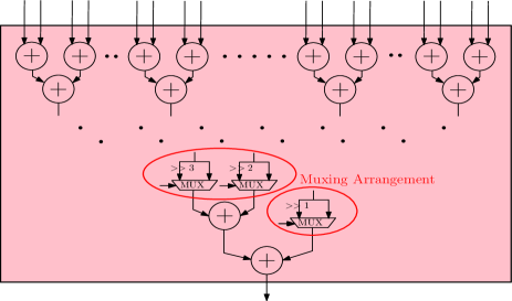
Fig. 10: Mux Add Tree Architecture

Note that this arrangement is independent of the filter length. In the adder tree architecture, the MAC terms which are scaled up by a factor of $2$ always come from second branch of the adder tree and hence this result is right shifted by one bit position to scale it down by $2$ and this doesn’t require any extra hardware.. Similarly the results of other two branches are right shifted by $2$ and $3$ bit positions. The choice of un-normalized HAAR wavelet has three advantages. We could exploit the redundancies in sliding wavelet transform through multiple levels of decomposition, we can get away with multipliers in calculating DWT and finally no special hardware required for scaling down the output. Multiplexing arrangement is necessary in the adder tree since we are folding the adder tree by a factor of $2$ (just like the DMPLMS case) and scaling is not needed during calculation of the denominator of proportional gain.

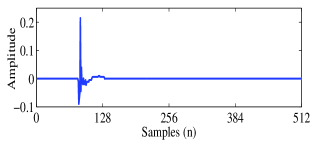
(a) Highly sparse system (sparse network echo path in ITU-T G.168), $S_{m}=0.8960$.

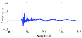
(b) Semi sparse system, $S_{m}=0.5560$.

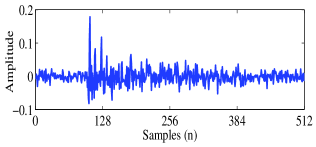
(c) Non-sparse system, $S_{m}=0.3486$.

Fig. 11: System impulse responses used in simulations.

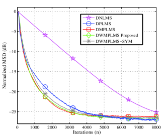
(a) White input sparse system.

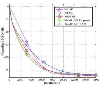
(b) White input semi sparse system.

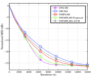
(c) White input disperse system

(d) color input sparse system.

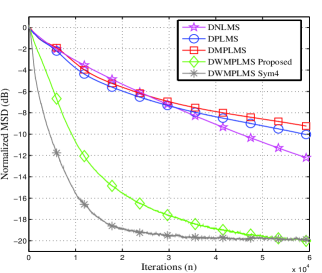
(e) color input semi sparse system.

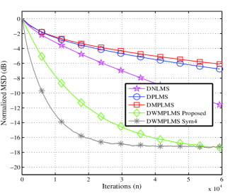
(f) color input disperse system.

Fig. 12: Performance comparisons.

IV-F Absolute power normalization

In this section we explain the third difference between DMPLMS and DWMPLMS architectures i.e. power normalization. After applying the orthogonal transform to the input, the input correlation matrix becomes diagonal but it doesn’t become identity matrix. Thus we need to normalize the correlation matrix with the power of each tap to make it identity matrix. The power of each tap is generally estimated using the following equation

$$\Psi_{i}(n)=\beta\Psi_{i}(n-1)+(1-\beta)(u_{T,i}(n))^{2},\mspace{4.0mu}0\leq i\leq(L-1).$$ (28)

However, this adds a significant area penalty as it effects all the taps and to simplify this we used absolute of the input instead of the square of the input and the new equation is shown below. We will show that the penalty for this approximation is negligible through simulations which are explained in the next section.

$$\Psi_{i}(n)=\beta\Psi_{i}(n-1)+(1-\beta)|(u_{T,i}(n))|,\mspace{2.0mu}0\leq i\leq(L-1).$$ (29)

We choose $\beta=0.125$ i.e. $\frac{1}{8}$ to avoid multiplication and this power estimation block is zoomed and shown in Fig. 9(a). In the next section we present detailed simulation results for the proposed algorithm.

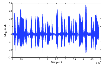
(a) Speech i/p.

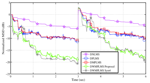
(b) Tracking performance.

Fig. 13: Performance comparison for speech input.

Table III: Synthesis results for TS18 180nm CMOS technology

Algorithm	# of taps	Clock freq.(MHz)	Leakage Power ($\mu$W)	Dynamic Power (mW)	Cell Area(kGE) a	Core Area($\mu m^{2})$
DLMS	$16$	$100$	$0.609$	$38.03$	$41.1$	$539290$
	$32$	$100$	$1.21$	$66.45$	$82.04$	$1085032$
	$64$	$100$	$2.43$	$114.39$	$164.1$	$2176258$
DPLMS	$16$	$100$	$0.802$	$33.36$	$49.57$	$650031$
	$32$	$100$	$1.57$	$61.95$	$97.26$	$1280869$
	$64$	$100$	$3.13$	$119.45$	$193.47$	$2558840$
DMPLMS	$16$	$100$	$0.867$	$47.67$	$52.88$	$693356$
	$32$	$100$	$1.70$	$91.72$	$103.83$	$1367065$
	$64$	$100$	$3.39$	$176.97$	$206.98$	$2736847$
DWMPLMS	$16$	$100$	$1.007$	$58.31$	$66.18$	$863061$
	$32$	$100$	$2.01$	$115.1656$	$130.84$	$1722799$
	$64$	$100$	$3.39$	$229.8$	$260.13$	$3441479$

• One gate equivalent corresponds to the size of a two input NAND gate of size $12.54\mu m^{2}$

V Simulation Results

For evaluating the performance of the DWMPLMS algorithm with all the proposed re-formulations and $3$-level un-normalized Haar wavelet, Experiments were performed in the context of echo cancelation which is the main application of sparse adaptive filters. we considered three systems of varying sparsity. The first system is a network echo path from G168 Recommendation and its impulse response can be considered to be very sparse since the associated sparseness measure is $0.89$, the second one is a semi sparse system with a sparsity measure of $0.5$ and third system is a disperse system with a sparsity of $0.3$. All the impulse responses have $512$ coefficients, using a sampling rate of $8$ kHz. All adaptive filters used in the experiments have the same length, i.e., L = $512$. The far-end signal (i.e., the input signal) is either a white Gaussian signal or a color input obtained by passing a white Gaussian input through an first order AR process with the pole at $0.95$ and speech sequence. The output of the echo path is corrupted by an independent white Gaussian noise (i.e., the background noise at the near-end) with $30$ dB echo-to-noise ratio (ENR). Adaptation step sizes for color input case are same as those mentioned in and for white case, $\mu_{dnlms}=\mu_{dmplms}=\mu_{dwmplms-sym4}=0.25,\mu_{dplms}=0.22,\mu_{dwmplms-proposed}=0.15$. Step sizes are adjusted such that steady state MSD is equal. We can see from Fig. 12, For both color and white inputs, as the sparsity decreases performance of DPLMS/DMPLMS becomes worse than that of DNLMS where as DWMPLMS is able to perform better or equal to the DNLMS. For the network echo cancelation which comes under color input sparse system, DWMPLMS significantly outperforms all the other three. We see that even if the sparsity or input correlation varies over wide range, DWMPLMS is able to perform consistently. We also evaluated the tracking performance (by changing the echo path in the midway by shifting the impulse response to the right by $12$ samples) of the proposed algorithm using the speech input shown in Fig. 13(a) for the sparse system and result is shown in Fig. 13(b). All other simulation parameters are same as that of color case and $\mu_{dnlms}=0.2,\mu_{dmplms}=\mu_{dplms}=50,\mu_{dwmplms-sym4}=2.5,\mu_{dwmplms-proposed}=1.1$. Please note that we need to adjust the step sizes depending on the input variance which is very low for the speech input and hence large value of $\mu$ for DMPLMS and DPLMS. We can see that the performances are similar to color case and we can conclude that DWMPLMS with U-HAAR 3-level decomposition is the robust VLSI solution to the echo cancelation with varying sparsity.

VI VLSI Implementation results and comparative study

In this section we provide the synthesis results of the proposed DWMPLMS, DMPLMS and DPLMS architectures and since there are no previous architectures reported for them in literature, we compare the results with standard DLMS to see how much is the complexity increase for the given convergence performance improvement. All the designs are implemented in Verilog, synthesized using Synopsys Design Compiler with TS$18$ standard cell library (Tower Semiconductor $180$nm CMOS technology). $16$-bit fixed point representation is considered for all the designs. Filter lengths of $16,32$ and $64$ are considered for comparing the scalability of time and area complexities and all the designs are targeted for $100$ MHz for fair comparison. The results are summarized in Table. III.

Compared to standard DLMS, re-formulated DPLMS has $20.53\%,18.04\%$ and $17.57\%$ more area complexity for $16,32$ and $64$ taps respectively. We see that the complexity increase is not exactly linear and it is intuitive because of overheads like adder tree, error calculation and G calculation blocks. Similarly DMPLMS has $28.56\%,25.99\%,25.75\%$ area complexity increase compared to DLMS. So roughly with $25\%$ increase in hardware we are getting 3x improvement in convergence performance in case of white input. Finally for color input when we consider DWMPLMS, it has $60.03\%,58.77\%,58.13\%$ area increase compared to DLMS complexity for $16,32$ and $64$ taps respectively. So we can conclude that with $58\%$ increase in hardware we are able to achieve 15x improvement in convergence for color input.

Finally we realized one higher order filter with 256-tap for the proposed DWMPLMS and the synthesis results at $100$MHz target frequency are shown in Table. IV and the detailed area break-up is shown in Table. V. We see that filter taps occupy most of the of area, followed by sliding HAAR unit which occupy around $10\%$ of the area. However, one can notice that the core area is on the higher side but thats because of $180$nm process and with more advanced technology nodes it will be scaled down accordingly.

Table IV: Synthesis Results of $256$-tap DWMPLMS

Parameter	Value
Clock freq	$100$ MHz
Dynamic Power	$417$ mW
Leakage Power	$16.9$ $\mu$W
Cell Area	$1037$ kGE
Core Area	$13.78$ mm2

Table V: Area Break Down of the Sub-blocks

	kGE	%
E Calculation	$1.62$	$0.16$
Adder Tree	$27.98$	$2.7$
$256$ Taps	$898.75$	$86.62$
Sliding HAAR unit	$109.1$	$10.52$
Total	$1037.45$	$100$

VII Conclusions and Future Work

Proportionate-type adaptive algorithms can significantly improve the convergence performance of the sparse adaptive filters compared to conventional LMS algorithm. However, the huge computational penalty associated with these algorithms make their VLSI realization a highly challenging task even with the most advanced technology nodes. By utilizing the fact that stochastic gradient algorithms are tolerant to approximations, we proposed several re-formulations in this paper to simplify the original PNLMS algorithms and compared the performances of these algorithms with those of the original algorithm and proposed an efficient VLSI architectures for these re-formulated algorithms. We also demonstrated that the DWMPLMS with the proposed $3$-level un-normalized HAAR wavelet is a robust VLSI solution for the practical echo cancelers with time varying sparsity. This is the first attempt to implement proportionate type algorithms in hardware and this result will motivate other researchers to explore more efficient hardware solutions to further improve the sparse adaptive filter architectures.

References

- [1] S. Weinstein, “Echo Cancellation in the Telephone Network”, in IEEE Communi- cations Magazine, vol. 15, iss. 1, pp. 8-15, Jan. 1977.
- [2] M. Stojanovic and J. Preisig, “Underwater Acoustic Communication Channels: Propagation Models and Statistical Characterization,” in IEEE Communications Magazine, pp. 84-88, January 2009.
- [3] L. Fan, C. He, D. Wang, and L. Jiang, “Efficient Robust Adaptive Decision Feedback Equalizer for Large Delay Sparse Channel,” in IEEE Trans. on Consumer Electronics, vol. 51, No. 2, pp. 449-456, May 2005.
- [4] C. Paleologu, J. Benesty, S. Ciochin, Sparse Adaptive Filters for Echo Cancellation, 2010, Morgan & Claypool.
- [5] D. L . Duttweiler, “Proportionate normalized least-mean-squares adaptation in echo cancelers”, in IEEE Trans. Speech Audio Process., vol. 8, no. 5, pp. 508-518, 2000.
- [6] S. Haykin and B. Widrow, Least-Mean-Square Adaptive Filters. Hoboken, NJ, USA: Wiley, 2003.
- [7] S. Gay, “An efficient, fast converging adaptive filter for network echo cancellation,” in Proc. 32nd Asilomar Conf. on Signal and System for Computing, vol. 1, 1998, pp. 394-398.
- [8] J. Benesty and S. L. Gay, “An improved PNLMS algorithm,” in IEEE Int. Conf. Acoust., Speech Signal Process. (ICASSP), vol. 2, pp.1881-1884, 2002.
- [9] H. Deng and M. Doroslovacki, “Proportionate Algorithms for Echo Cancellation”, in IEEE Trans. on Signal Processing., vol. 54, no. 5, pp. 1794-1803, May 2006.
- [10] H. Deng and M. Doroslovacki, “Improving convergence of the PNLMS algorithm for sparse impulse response identification,” in IEEE Signal Process. Letters, vol. 12, no. 3, pp. 181-184, 2005.
- [11] K. Wagner, M. Doroslovacki, and H. Deng “Convergecne of proportionate-type NLMS adaptive filters and choice of gain matrix,” Proc. 40th Asilomar on Sig- nals, Systems, and Computers, Pacific Grove, CA, Oct. 29 - Nov. 1, 2006.
- [12] H. Deng and M. Doroslovacki, “Wavelet-Based MPNLMS Adaptive Algorithm for Network Echo Cancellation,” EURASIP Journal on Audio, Speech, and Music Processing., vol. 2007, Oct. 2007.
- [13] Dyba, Roman A and He, Perry P and Pessoa, Lúcio FC, Network Echo Cancellers and Freescale Solutions Using the StarCore SC140 Core , 2004, Freescale Application Note AN2598/D.
- [14] Chen, Jie, Efficient VLSI Architectures for High-Speed Ethernet Transceivers, , 2008, ProQuest.
- [15] V. C. Gogineni, S. Mula, R. L. Das and M. Chakraborty, “Performance analysis of proportionate-type LMS algorithms,“ 2016 Signal Processing: Algorithms, Architectures, Arrangements, and Applications (SPA), Poznan, Poland, 2016, pp. 177-181.
- [16] G. Long, F. Ling, and J. G. Proakis, “The LMS algorithm with delayed coefficient adaptation,“ in IEEE Trans. Acoust., Speech, Signal Process., vol. 37, pp. 1397-1405, Sep. 1989.
- [17] P. K. Meher and S. Y. Park, “Area-Delay-Power Efficient Fixed-Point LMS Adaptive Filter With Low Adaptation-Delay,”in IEEE Trans., Very Large Scale Integr. (VLSI) Syst., vol. 22, no. 2, pp. 362-371, 2014.
- [18] T. C. Denk and K. K. Parhi, “Exhaustive scheduling and retiming of digital signal processing systems,“ in IEEE Trans., Circuits Syst. II, Analog Digit. Signal Process.,, vol. 45, no. 7, pp. 821-838, Jul 1998.
- [19] S. F. Oberman and M. Flynn, “Division algorithms and implementations,“ IEEE Trans. Comput., vol. 46, no. 8, pp. 833-854, Aug. 1997.
- [20] J. N. Mitchell, Jr., “Computer multiplication and division using binary logarithms,“ in IRE Trans. Electron. Comput., vol. 11, no. 11, pp. 512-517, Aug. 1962.
- [21] D. F. Marshall, W. K. Jenkins and J. J. Murphy, “The use of orthogonal transforms for improving performance of adaptive filters,“ in IEEE Trans., Circuits Syst.,, vol. 36, no. 4, pp. 474-484, Apr 1989.
- [22] K. C. Ho and S. D. Blunt, ”Adaptive sparse system identification using wavelets,” in IEEE Trans., Circuits Syst. II, Analog Digit. Signal Process.,, vol. 49, no. 10, pp. 656-667, Oct 2002.
- [23] G. Strang and T. Nguyen,Wavelets and Filter Banks. Cambridge, MA: Wellesley-Cambridge , 1996.
- [24] Samir Attallah, “The Wavelet Transform-Domain LMS Algorithm: A More Practical Approach,“ in IEEE Trans., Circuits Syst. II, Analog Digit. Signal Process.,, vol. 47, no. 3, pp. 209-213, Mar 2000.