Terrestrial planet formation: Dynamical shake-up and the low mass of Mars

Abstract

We consider a dynamical shake-up model to explain the low mass of Mars and the lack of planets in the asteroid belt. In our scenario, a secular resonance with Jupiter sweeps through the inner solar system as the solar nebula depletes, pitting resonant excitation against collisional damping in the Sun’s protoplanetary disk. We report the outcome of extensive numerical calculations of planet formation from planetesimals in the terrestrial zone, with and without dynamical shake-up. If the Sun’s gas disk within the terrestrial zone depletes in roughly a million years, then the sweeping resonance inhibits planet formation in the asteroid belt and substantially limits the size of Mars. This phenomenon likely occurs around other stars with long-period massive planets, suggesting that asteroid belt analogs are common.

1 Introduction

The Sun’s rocky planets arose from many small dust particles that were concentrated into a few larger ones (Safronov, 1969). Although this process of coagulation, accretion and merging is slow, it is efficient (e.g., Chambers & Wetherill, 1998; Kenyon & Bromley, 2006), creating Venus and Earth out of the primordial dust in the inner solar nebula. Yet just beyond 1 AU, Mars grew to only a tenth of an Earth mass. The asteroid belt, with just a few percent of a Lunar mass in total, has no planets at all. Some aspect of planet formation, either its efficiency or the abundance of solids, prevented the growth of Earth-mass planets beyond 1 AU. To learn the history of our solar system and to predict the prevalence of rocky planets throughout the Universe, it is important to understand the physical processes responsible for a low-mass Mars.

If the Sun’s protoplanetary disk was truncated just past the Earth’s orbit, the low mass of Mars and the depletion of solids in the asteroid belt are natural outcomes (Jin et al., 2008; Hansen, 2009; Izidoro et al., 2014; Walsh & Levison, 2016; Haghighipour & Winter, 2016). Possibly, the disk was born that way. However, dynamical excitation and depletion can also explain the orbital architecture of the inner solar system (Izidoro et al., 2015). Long-range interactions with Jupiter and Saturn may provide these excitations (Wetherill, 1992; Nagasawa et al., 2005; Raymond et al., 2009). Alternatively, the gas giants themselves might have migrated through the disk, drifting inward to the terrestrial zone and then outward in a “Grand Tack” that cleared material in their path (Walsh et al., 2011).

After the formation of the gas giants, the remaining gas disk continues to dissipate from viscous diffusion, photoevaporation, and erosion by a stellar wind (e.g., Chambers, 2009; Alexander & Armitage, 2009; Matsuyama et al., 2009). In the late stages of depletion, the gravity of the disk and the gravity of the gas giants conspire to generate secular resonances in the inner solar system (Heppenheimer, 1980; Ward, 1981; Lecar & Franklin, 1997; Nagasawa et al., 2000). Within the $\nu_{5}$ resonance, where the local apsidal precession rate matches Jupiter’s rate of precession, orbiting bodies experience repeated eccentricity kicks. As the disk’s gravity fades, the location of this resonance sweeps inward, pumping the eccentricity of all objects in its path (Nagasawa et al., 2005; Thommes et al., 2008). This dynamical “shake-up” sculpts the inner solar system, leaving its imprint on Mars and the asteroid belt (O’Brien et al., 2007; Nagasawa et al., 2007; Haghighipour & Winter, 2016).

Timing is an important constraint for assessing the impact of the Grand Tack, dynamical shake-up, and other sculpting mechanisms. Calculations of planet formation for the inner solar system predict that Mars-size protoplanets form on million-year time scales at 1.5 AU (Chambers & Wetherill, 1998; Kenyon & Bromley, 2006; Raymond et al., 2009). Radiometric data support this idea, indicating a fully assembled Mars within $\sim$4 Myr (Dauphas & Pourmand, 2011). With depletion of the reservoir of gas in $\sim$1–5 Myr (Haisch et al., 2001; Kennedy & Kenyon, 2009; Wang et al., 2017), the gas giants probably form before Mars reaches its final mass. Thus, within a few million years of the collapse of the solar nebula, the gas giants were largely in place, the gas disk was diminished, and Mars was near completion.

Compared to these evolutionary time scales, the Grand Tack model operates on a tight schedule (Walsh et al., 2011). In this picture, the gas giants fully form within a million years and begin to migrate within an undepleted gaseous disk. After Jupiter and Saturn begin their return trip through the gaseous disk — the “tack” — the gas beyond the asteroid belt must dissipate rapidly to end outward migration. The outcome of this process is a reduced surface density of solids beyond 1 AU, leaving a small Mars and a dynamically excited, depleted asteroid belt. While compelling, this picture requires careful synchronization between gas giant formation, the evolution of the gas disk, and the growth of solids at 1–3 AU (Raymond & Morbidelli, 2014).

In contrast, the main timing constraints for dynamical shake-up are that (i) the gas disk vanishes inside 5–10 AU after the formation of Jupiter and (ii) the disk inside the Kuiper belt dissipates on time scales of millions of years (Nagasawa et al., 2000). The dissipation rate governs (i) how quickly the $\nu_{5}$ and other resonances sweep through the inner solar system and (ii) how long individual objects experience the resonance. A resonance that sweeps rapidly may not shake up anything; a slowly moving resonance can lead to dynamical ejections. For disk dissipation time scales in the range favored by observations (e.g., Haisch et al., 2001; Kennedy & Kenyon, 2009; Bell et al., 2013; Pfalzner et al., 2014; Ribas et al., 2015; Wang et al., 2017), resonances sweep through slowly enough to make an impact with little sensitivity to the way the disk dissipates (Nagasawa et al., 2000). Therefore, a dynamical shake-up almost certainly played an important role in the formation of the solar system.

Here, we consider the possibility that the low mass of Mars and the asteroid belt might result directly from the dynamical shake-up, without the need for large-scale migration of the gas giants. Although previous studies (Nagasawa et al., 2005; O’Brien et al., 2007; Nagasawa et al., 2007; Thommes et al., 2008) showed promising results, both the shake-up and the formation of Mars were thought to have occurred after $\sim 5$–10 Myr. Armed with more recent estimates of Mars’ formation time, we propose that the shake-up happened earlier, when planet formation in the inner solar system was far from complete. To assess the impact of this early shake-up requires tracking the evolution of planetesimals, including the physics of coagulation. Collisional damping is also critical to the outcome, as it counteracts dynamical excitations from sweeping resonances. Our new contribution is a set of calculations that include these effects, performed with our planet formation code, Orchestra (Bromley & Kenyon, 2006, 2011, 2013).

We organize this paper as follows. In §2 we consider orbital dynamics in the inner solar system, including the nature of particle orbits in the presence of outer gas giants and the mechanics of a sweeping resonance driven by an evolving gas disk. We incorporate these phenomena in our planet formation code, summarized in §3. In §4, we present the results from two extensive multiannulus simulations that compare rocky planet formation with and without a dynamical shake-up. In our conclusion, §6, we summarize the advantages and limitations of dynamical shake-up for explaining the low mass of Mars. We also discuss the implications of our results for terrestrial planet formation elsewhere in the Universe.

2 Orbital dynamics in the inner solar system

We first consider the orbital dynamics of growing planetesimals and protoplanets within the context of the shake-up model. Our motivation here is to understand how to include the gravitational effects of giant planets and a gas disk in our planet formation code. First, we focus on Jupiter, which produces a significant time varying gravitational potential that affects orbital motion throughout the solar system. Outside of its Hill sphere, however, there are sets of “most-circular” orbital paths that enable disks of particles to be dynamically cold. Along these orbits, stirring by Jupiter is negligible. Thus, planet formation in the inner solar system can proceed as if Jupiter were not there. A similar situation exists for binary stars (Bromley & Kenyon, 2015).

The presence of a massive gaseous disk in the Sun–Jupiter binary complicates this simple picture. From secular perturbation theory, orbital precession driven by Jupiter and the disk can lead to secular resonances that excite eccentricities of planetesimals and protoplanets. The resonance location changes along with the disk potential as the disk evolves. Although aerodynamic drag and dynamical friction with the gas can (i) damp eccentricity and (ii) remove small particles from the system, strong secular resonances that sweep through the disk can generate large orbital eccentricity $e$ that may persist even after the disk vanishes.

In this section, we cover orbital dynamics in the presence of an outer giant planet, an evolving gas disk, and the sweeping resonances they produce. Following Nagasawa et al. (2005) and Thommes et al. (2008), we focus here on the strong $\nu_{5}$ apsidal resonance, although nodal resonances may also contribute to a shake-up (e.g., Haghighipour & Winter, 2016). We include several examples that illustrate how a sweeping resonance might have affected protoplanetary orbits in the terrestrial zone of the young Sun.

2.1 Orbit solutions and “most circular” paths

To quantify the orbits of small bodies in the inner solar system, we first consider the isolated influence of Jupiter, treating it as a binary partner to the Sun. Following the theory of Lee & Peale (2006) and Leung & Lee (2013), we assume that particle orbits make small excursions about a guiding center on a circular track around the Sun. We then solve equations of motion to linear order in these excursion distances. Lee & Peale (2006) and Leung & Lee (2013) originally focused on circumbinary systems where the eccentricities of all objects, including the binary, are low. Here we extend this theory to the intrabinary (circumprimary) case.

Using the prescription in Appendix A, we obtain orbit solutions for tests particles interior to Jupiter’s orbit. For orbital excursions that are small compared to Jupiter’s semimajor axis ${a_{\rm J}}$ and for low orbital eccentricities $e$, orbit solutions are

$$R(t) \approx {R_{\rm g}}\left[1-e_{\rm free}\cos(\kappa_{\rm e}t+\psi_{e})-e_{\rm force}\cos({\Omega_{\rm g}}t)-F(t,{R_{\rm g}},)\right],$$ (1)

$$\phi(t) \approx {\Omega_{\rm g}}\left[1+\frac{2e_{\rm free}}{\kappa_{\rm e}}\sin(\kappa_{\rm e}t+\psi_{e})+\frac{2e_{\rm force}}{{\Omega_{\rm g}}}\sin({\Omega_{\rm g}}t)+G(t,{R_{\rm g}})\right],$$ (2)

$$z(t) \approx {R_{\rm g}}i\sin(\kappa_{\rm i}t+\psi_{i})$$ (3)

where $R$, $\phi$ and $z$ are cylindrical coordinates with the origin at the Sun and with Jupiter in the $z=0$ plane. We define the other variables and functions according to how they contribute to the test particle’s motion:

1. The radius ${R_{\rm g}}$ defines the circular path of the particle’s guiding center, which has an orbital frequency ${\Omega_{\rm g}}$;

2. The “free eccentricity” $e_{\rm free}$ and inclination $i$ describe motion in the epicyclic approximation of Keplerian orbits around the Sun, with the angular frequencies $\kappa_{\rm e}$ and $\kappa_{\rm i}$, respectively, which differ slightly from ${\Omega_{\rm g}}$;

3. The “forced eccentricity” $e_{\rm force}$ corresponds to epicyclic motion in the Sun-Jupiter plane, driven at angular frequency ${\Omega_{\rm g}}$ by Jupiter; and

4. The functions $F$ and $G$ quantify additional modes of oscillation that depend on harmonics of Jupiter’s mean motion and the synodic frequency of Jupiter and the test particle.

The remaining variables, $\psi_{e}$ and $\psi_{i}$, are phase angles defined to apsidally align the test particle with Jupiter at $t=0$.

Because a test particle’s epicyclic frequency $\kappa_{\rm e}$ and vertical frequency $\kappa_{\rm i}$ differ from the mean motion ${\Omega_{\rm g}}$, its argument of perihelion and ascending node precess (Appendix A). For ${a_{\rm J}}$ = 5.2 AU, the apsidal precession rate is

$$\dot{\varpi}_{\rm p,J}\equiv{\Omega_{\rm g}}-\kappa_{\rm e}\approx\frac{3}{4}{\Omega_{\rm kep}}\frac{M_{J}}{M_{\odot}}\frac{a^{3}}{{a_{\rm J}}^{3}}\approx 36\times\left[\frac{a}{\textrm{\small 1\,AU}}\right]^{3/2}\ \textrm{rad/Myr,}$$ (4)

where we have replaced ${R_{\rm g}}$ with orbital distance $a$, and the subscript (${p,J}$) specifies precession of the test particle — representing a planetesimal or protoplanet — as a result of Jupiter’s influence. The corresponding apsidal precession time is

$$T_{p,J}\approx 0.17\left[\frac{a}{\textrm{\small 1\,AU}}\right]^{-3/2}\ \textrm{Myr.}$$ (5)

This time scale is (i) short compared to the 3–5 Myr lifetime of the gaseous disk (e.g., Bell et al., 2013; Ribas et al., 2015) and (ii) comparable with the time scale for Jupiter and Saturn to migrate through the disk (e.g., Walsh et al., 2011).

The forced eccentricity imposed by Jupiter on a small body orbiting interior to the gas giant is

$$e_{\rm force}\approx\frac{5}{4}\frac{a}{{a_{\rm J}}}{e_{\rm J}}\approx 0.012\left[\frac{a}{\textrm{\small 1\,AU}}\right]\left[\frac{{e_{\rm J}}}{\textrm{\small 0.049}}\right]\ \ \ \ \ \textrm{($a\ll{a_{\rm J}}$)},$$ (6)

where ${e_{\rm J}}$ is Jupiter’s eccentricity. Unlike the free eccentric motion, the forced eccentric mode remains apsidally aligned with Jupiter’s orbit.

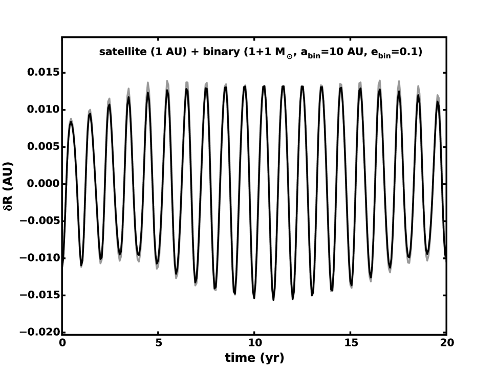
Figure 1: Radial position of a test particle (a “satellite”, such as a planetesimal or protoplanet) on a most circular orbit about a star in a stellar binary system. The two stars have mass equal to 1 $M_{\odot}$ and orbit with semimajor axis $a$ = 10 AU and eccentricity $e_{\rm bin}=0.1$. The particle’s average distance from its primary host is ${R_{\rm g}}=1$ AU. The radial fluctuations show the rapid forced eccentric oscillations plus slower modulations from the binary’s epicyclic motion. For the Sun-Jupiter system, the rapid radial oscillations are similar to the curve in the plot, but the slower modulations are not evident.

From the orbit solutions, planetesimal and protoplanets follow “most circular” paths when $e_{\rm free}$ goes to zero. These trajectories are generalizations of circular orbits around an isolated star that allow for ebb and flow in response to gravitational perturbations from Jupiter (e.g., Lee & Peale, 2006; Youdin et al., 2012; Bromley & Kenyon, 2015). Figure 1 illustrates most-circular orbit solutions for an intrabinary planetesimal in the extreme case of an equal-mass stellar binary. To achieve these orbits, swarms of planetesimals collisionally damp, ridding themselves of free eccentricity. The time scale for this dynamical cooling process is limited by the precession time of the free eccentricity, Equation (5), as well as the collision time. Furthermore for settling to occur, the binary eccentricity must be modestly low (${e_{\rm J}}\lesssim 0.5$), so that most-circular orbits are nested and non-intersecting (see below).

2.2 Orbits in a massive gas disk

To include a gaseous disk in our planet formation calculation, we adopt a simple axisymmetric model, with surface density

$$\Sigma(a,t)=\Sigma_{0}\exp(-t/\tau)\left(\frac{a}{a_{0}}\right)^{-n}\ \ \ \ \ \ \ \ \ \text{($a_{in}<a<a_{out}$ [0 otherwise])},$$ (7)

where $a$ is the distance from the Sun, $t$ is time, $\Sigma_{0}$, $n$ and $\tau$ are constants, $a_{in}$ and $a_{out}$ are inner and outer disk radii, and $a_{0}\equiv 1$ AU. By setting $\Sigma_{0}=2000$ g/cm² and $n=1$, we adopt a model similar to the Minimum Mass Solar Nebula (MMSN; Weidenschilling, 1977b; Hayashi, 1981), which is comparable in mass with some disks observed around young stars (e.g., Andrews et al., 2009, 2010; Dent et al., 2013; Andrews et al., 2013). Choosing a time scale $\tau\sim 1$–3 Myr reproduces observed disk dissipation rates if the disk erodes “uniformly” over its surface (Haisch et al., 2001; Williams & Cieza, 2011). Alternatively, the disk may erode from the inside out with an inner disk radius

$$a_{in}(t)=a_{in}(0)+{\dot{a}_{{\rm in}}}t,$$ (8)

where ${\dot{a}_{{\rm in}}}$ is a constant expansion rate. Theory (Owen et al., 2012; Clarke & Owen, 2013) and observations of transition disks (Calvet et al., 2005; Currie et al., 2008; Andrews et al., 2011) suggest that ${\dot{a}_{{\rm in}}}\gtrsim 10$ AU/Myr (see also Owen, 2016). Here, our disk models either decay uniformly with a finite $\tau$ or they have an expanding inner edge, but not both. In all cases, we fix $a_{out}$ to be 100 AU. Results described below are insensitive to this choice.

For the vertical structure of the disk, we set the characteristic density in the disk as $\rho\sim\Sigma/h$ with vertical scale height

$$h=h_{0}\left(\frac{a}{a_{0}}\right)^{5/4},$$ (9)

and $h_{0}=0.04$ AU (Kenyon & Hartmann, 1987; Andrews & Williams, 2007; Andrews et al., 2009).

To model the spatial distribution of solids, we assume that the surface density $\Sigma_{s,0}=10$ g/cm² and $n=1.5$ for material inside the snow line. Solids in the terrestrial zone then comprise about 0.5% of the initial disk mass. Solid particles have a size-dependent scale height, which depends on the relative importance of settling, gas drag, and gravitational stirring (Weidenschilling, 1980; Goldreich et al., 2004; Chiang & Youdin, 2010). For simplicity, we assume that the surface density of solids does not deplete with the gas, but evolves independently of the gas disk.

Finally, we assume that Jupiter and Saturn create and maintain gaps in both the gas and solid particle disks. Thus we set the surface density to zero in annuli of width 1 AU, centered on each of the gas giants. This point is important because the sense of apsidal precession of the gas giants themselves depends on whether they are embedded in the disk. We discuss this issue next.

2.2.1 Disk gravity

The non-Keplerian potential of a massive disk also results in orbital precession. Aside from contributing to the location of secular resonances, the time-varying gravitational potential of the disk as it dissipates is the key to resonant sweeping and the dynamical shake-up model. While we use a grid-based method to handle disk gravity in our orbit solvers (Bromley & Kenyon, 2011), analytical estimates offer some insight into the impact of a disk on solid objects.

For a simple, power-law disk with no gaps, the potential at distance $a$ within the bulk of the disk is

$$\Phi_{d}(a)\approx\begin{cases}2\pi G\Sigma_{0}\exp(-t/\tau)a_{0}\log(a/a_{0})&\ \ \ \ \ \ \ \ \textrm{($n=1$; gas)}\\ -8.8\pi G\Sigma_{0}\exp(-t/\tau)a_{0}(a/a_{0})^{1.5}&\ \ \ \ \ \ \ \ \textrm{($n=1.5$; solids)}\end{cases}$$ (10)

(Appendix A of Bromley & Kenyon, 2011). This potential induces apsidal precession at a rate of

$$\dot{\varpi}_{\rm p,d}\approx-\pi\frac{a^{2}\Sigma(a,t)}{M}{\Omega_{\rm kep}}\ \ \ \ \ \ \ \ \ \ \ \textrm{(extended power-law disk),}$$ (11)

where the subscript (${p,d}$) signifies the precession of a planetesimal (or protoplanet) caused by the disk (Appendix B, Equation (B6)). This expression is exact for $n=1$ and is accurate to about 10% for $n=1.5$ (e.g., Rafikov, 2013; Silsbee & Rafikov, 2015). The negative sign indicates that a planetesimal embedded in a disk has an apside that precesses in a sense opposite to its orbital motion. The precession period is

$$T_{p,d}\approx 0.14\left[\frac{a}{\textrm{\small 1\,AU}}\right]^{5/2}\left[\frac{\Sigma(a,t)}{\textrm{\small 20\,g/cm${}^{2}$}}\right]^{-1}\ \textrm{Myr}\ \ \ \ \ \ \ \ \ \ \ \textrm{($a_{in}\ll a\ll a_{out}$, $n=1$)}.$$ (12)

We choose numerical factors to highlight conditions where the precession from the disk is comparable to the precession induced by Jupiter (Equation (5)). Similar precession periods lead to resonances and the dynamical shake-up.

The disk gravity affects the gas giants as well, but because these planets can clear gaps, the nature of their precession is different. For Jupiter centered in a 1 AU full-width gap, the precession rate is

$$\dot{\varpi}_{\rm J,d}=1.25\pi\frac{{a_{\rm J}}^{2}\Sigma({a_{\rm J}})}{M}{\Omega_{\rm J}}$$ (13)

where ${\Omega_{\rm J}}$ is the angular speed of Jupiter’s orbit. We obtain the numerical coefficient from numerical experiments (see below) using a disk with a gap and a finite scale height. This value is within a factor of about two of the analytical estimate of Nagasawa et al. (2005, Equation (23) therein) for an infinitesimally thin disk.

To describe scenarios in which the circumsolar gas erodes from the inside out, we estimate the precession rate of a planetesimal or protoplanet using Equation (4) for the orbit-averaged precession induced by a planetary perturber. By substituting $2\pi\Sigma a^{\prime}da^{\prime}$ for the perturber mass and integrating over orbital distance $a^{\prime}$,

$$\dot{\varpi}_{\rm p,d}\approx\frac{3}{4}{\Omega_{\rm kep}}\frac{\pi a_{in}^{2}\Sigma(a_{in})}{M_{\odot}}\frac{a^{3}}{a_{in}^{3}}\ \ \ \ \ \ \ \ \ \ \ \textrm{($a\ll a_{in}$, $n=1$; {inner cavity})}.$$ (14)

This expression is valid when the inner edge of the disk is far beyond the orbit of the planetesimal or protoplanet. When resonances sweep through the terrestrial zone, the inner edge of the disk is well outside of Saturn’s orbit. This expression is then a useful approximation. The precession period is

$$T_{p,d}=0.19\left[\frac{a}{\textrm{\small 1\,AU}}\right]^{-3/2}\left[\frac{\Sigma(a_{in})}{\textrm{\small 200\,g/cm${}^{2}$}}\right]^{-1}\left[\frac{a_{in}}{\textrm{\small 10\,AU}}\right]\ \textrm{Myr.}\ \ \ \ \ \ \ \ \ \ \ \textrm{($a\ll a_{in}$; $n=1$)},$$ (15)

where the choice of numerical factors reflects the fact that the surface density of a MMSN disk at 10 AU is 200 g/cm² when $n$ = 1.

In comparing an extended power law disk and a disk with an inner cavity, a planetesimal or protoplanet within a disk cavity or gap precesses in the same sense as its orbital motion, while an object embedded within a power-law disk precesses in the opposite sense. Despite these differences, in our models the magnitude of $\dot{\varpi}_{\rm p,d}$ generally decreases monotonically with $a$. Furthermore, the effect of the disk on the precession of a planetesimal in the terrestrial zone relative to Jupiter is fairly insensitive to the way the disk dissipates in our models.

For disks with finite spatial extent and gaps, we use a numerical approximation to quantify the gravitational acceleration. After dividing the disk into 2500 annuli spanning orbital distances from 0.1 AU to 100 AU, we evaluate the disk gravity at each annulus and derive real-time acceleration evaluations by interpolation (see Bromley & Kenyon, 2011). In this way we can accommodate a wide range of disk surface density profiles. Our code can perform these calculations in 3-D around an axisymmetric disk. However, our focus here is on eccentricity pumping, and we work only in the disk midplane, defined to have no inclination with respect to the Sun-Jupiter binary.

2.2.2 Resonant excitations

Even with only modest eccentricity, Jupiter continuously pumps the eccentricity of objects throughout the solar system. The pumping rate is

$${\dot{e}_{{\rm pump}}}\approx\frac{15}{16}{\Omega_{\rm kep}}\frac{M_{J}}{M_{\odot}}\frac{a^{4}}{{a_{\rm J}}^{4}}\,{e_{\rm J}}\approx 0.44\times\left[\frac{a}{\textrm{\small 1\,AU}}\right]^{5/2}\left[\frac{{e_{\rm J}}}{\textrm{\small 0.049}}\right]\ \textrm{Myr${}^{-1}$}$$ (16)

(Appendix B, Equation (B5)). If a planetesimal experiences apsidal precession relative to Jupiter, then its orbit can be stable, despite the pumping: Precession constantly reorients the planetesimal’s orbit, preventing the eccentricity from coherently building up. The forced eccentric motion arises from a balance between pumping and precession; the more rapid the relative precession, the smaller the forced eccentricity.

By modulating the precession rates of both Jupiter and a planetesimal, a massive gas disk complicates this picture. The forced eccentricity becomes (Appendix B)

$$e_{\rm force}\approx\frac{5}{4}\left[\frac{\dot{\varpi}_{\rm p,J}}{(\dot{\varpi}_{\rm p,J}+\dot{\varpi}_{\rm p,d})-\dot{\varpi}_{\rm p,J}}\right]\frac{a}{{a_{\rm J}}}{e_{\rm J}},$$ (17)

where $\dot{\varpi}_{\rm J,d}$ is the apsidal precession rate of Jupiter from the disk. Thus, the denominator describes the precession rate of the planetesimal relative to Jupiter.

This form of the forced eccentricity has implications for the ability of a swarm of planetesimals to settle on most circular orbits. Near a secular resonance, where planetesimals and Jupiter precess at the same rate, the forced eccentricity diverges and orbits necessarily cross. Thus, there are regions near the resonance where solid material cannot settle onto most circular orbits. To prevent orbit crossing,

$$\left|e_{\rm force}+a\frac{de_{\rm force}}{da}\right|<1~{},$$ (18)

which comes from the requirement that the perihelion distance of planetesimals on adjacent most-circular orbits do not overlap. In regions where this condition is met, away from secular resonances, non-intersecting most circular orbits exist, and small solids can settle to a dynamically cold state.

2.2.3 Resonant sweeping

We derive more general circumstances for secular resonances by expressing the precession rate of a planetesimal (or protoplanet) relative to Jupiter as

$$\dot{\varpi}_{\rm p}-\dot{\varpi}_{\rm J} = \dot{\varpi}_{\rm p,J}+\dot{\varpi}_{\rm p,S}+\dot{\varpi}_{\rm p,d}-\dot{\varpi}_{\rm J,S}-\dot{\varpi}_{\rm J,d},$$ (19)

where $\dot{\varpi}_{\rm p,S}$ and $\dot{\varpi}_{\rm J,S}$ are the precession rates that Saturn imposes on the planetesimal and Jupiter, respectively. When $\dot{\varpi}_{\rm p}=\dot{\varpi}_{\rm J}$, the planetesimal experiences the $\nu_{5}$ secular resonance with Jupiter. The location of the resonance varies with the evolution of the disk. In a very massive disk, planetesimal orbits precess so rapidly that no resonance exists within the orbit of Jupiter ($|\dot{\varpi}_{\rm p}|\gg|\dot{\varpi}_{\rm J}|$ for all $a<{a_{\rm J}}$). As the disk dissipates, the planetesimal precession slows, until the effect of precession from Jupiter’s gravity kicks in. Because Jupiter causes precession most strongly at orbital distances closest to it, the $\nu_{5}$ resonance appears first beyond the terrestrial zone, and sweeps inward as the disk fades away, settling just beyond the orbit of Venus.

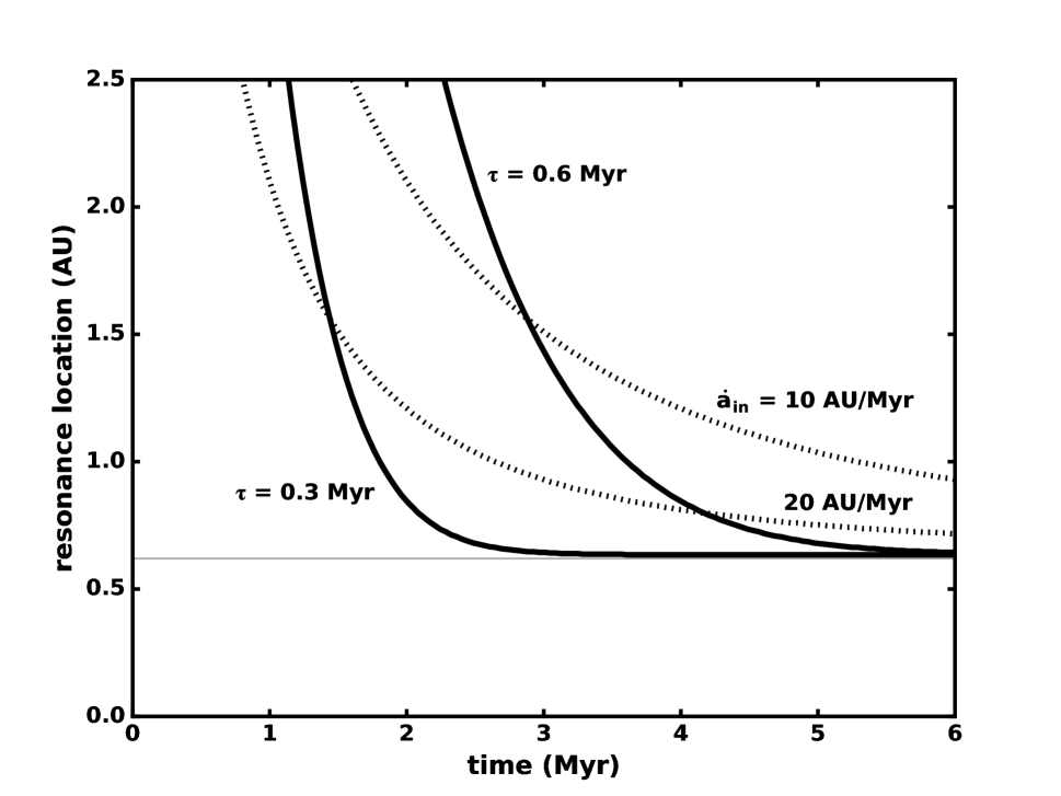
Figure 2: The location of the $\nu_{5}$ secular resonance in two types of disk evolution models with Jupiter (Saturn) in orbit at $a_{J}$ = 5.20 AU ($a_{S}$ = 9.58 AU). The solid curves show the orbital distance where (i) a test particle’s apsidal precession rate matches Jupiter’s and (ii) the gas disk depletes uniformly with depletion time scale $\tau$. The dotted curves correspond to inside-out depletion of the disk, where ${\dot{a}_{{\rm in}}}$ is the expansion rate of the disk’s inner edge. The curves come from analytical approximations that include the gravity of the disk, Saturn’s influence, and a Jupiter which clears a gap in the disk if the disk’s inner edge is within Jupiter’s orbit.

Figure 2 illustrates the evolving location of the $\nu_{5}$ resonance in the uniform depletion and inside-out disk dissipation models. To estimate this location, we calculate eigenfrequencies of precession for the Jupiter-Saturn system in secular theory (e.g., Heppenheimer, 1980; Nagasawa et al., 2000), adopting the present-day orbital configuration of the two gas giants ($a_{J}$ = 5.20 AU; $a_{S}$ = 9.58 AU). The figure shows that the timing and location of the sweeping resonance depends on the form of disk dissipation. Slower dissipation yields a more slowly sweeping resonance. The resonance sweeps through the inner solar system more slowly with inside-out dissipation than with homologous disk depletion.

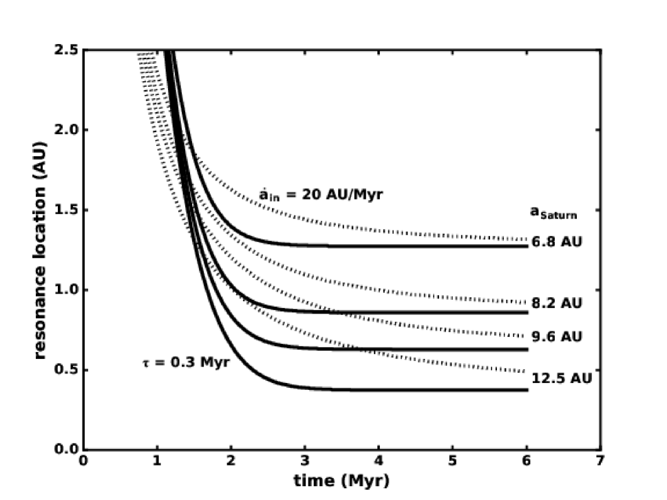
Figure 3: The location of the $\nu_{5}$ secular resonance for several different orbits of Saturn. As in the preceding Figure, the solid curves correspond to uniform disk depletion, while the dotted curves correspond to inside-out depletion of the disk. Parameters for each model are shown. For each disk depletion model, the position of the resonance is calculated with Saturn at one of four positions: Two positions correspond to the 3:2 and 2:1 Jupiter-Saturn commensurabilities near 6.8 AU and 8.2 AU respectively, while the third is near Saturn’s present-day orbit. The fourth position for Saturn is chosen as an example when the Jupiter-Saturn orbital separation was greater than the present day value. In all cases, Jupiter is at an orbital distance of 5.2 AU.

Figure 3 highlights the role of Saturn in setting the pace and timing of resonance sweeping. Although the final position of the resonance is sensitive to Saturn’s orbital distance, the timing of sweeping beyond 1 AU is rather insensitive to $a_{S}$. In inside-out dissipation with Jupiter and Saturn near the 3:2 orbital commensurability, the $\nu_{5}$ resonance settles at roughly 1.3 AU; the sweep rate is then comparatively slow as the resonance crosses Mars’ orbit. The disk model then mimics a more slowly evolving disk. In calculations with larger $a_{S}$, the resonance sweeps rapidly through Mars’ orbit independent of the exact value of $a_{S}$.

These results demonstrate that outcomes of dynamical shake-up calculations are not sensitive to $a_{S}$. Whether Saturn orbits in its current location as in classical models (e.g., Haghighipour & Winter, 2016) or in a more compact configuration with Jupiter as in the Nice model (Tsiganis et al., 2005), the $\nu_{5}$ resonance passes through the asteroid belt and the orbit of Mars. The pace and timing of resonance sweeping are more sensitive to the form and timing of disk evolution than the orbit of Saturn.

2.2.4 Dynamical friction and eccentricity damping

In addition to generating an overall axisymmetric potential, the gas disk produces gravitationally important density wakes as it responds to the local gravity of large planetesimals, protoplanets and planets. By creating these wakes, a massive object experiences eccentricity damping and radial migration through the disk (Lin & Papaloizou, 1979; Goldreich & Tremaine, 1980; Lin & Papaloizou, 1986; Artymowicz, 1993; Ward, 1997). Eccentricity damping arises because of the “downstream” density enhancements caused by Rutherford scattering as a planet plows through the gas disk. Once it has circularized, the planet feels torque from the gas in Keplerian flows streaming by, flowing in one direction on interior orbits and the other direction on exterior orbits. The slight torque differential causes the planet to drift radially. The exact mechanism depends on whether the planet is massive enough to clear a gap in the disk (Ward, 1997). Small planets unable to generate a gap experience type I migration, which typically is slow in the terrestrial zone compared to the disk lifetimes considered here. More massive planets that open a gap undergo Type II migration, which operates on viscous time scales that are short compared to the disk depletion time scale in a massive disk.

We focus first on eccentricity damping. The damping time scale is

$$\tau_{\rm damp} \equiv \frac{e}{\dot{e}}=\frac{1}{{\Omega_{\rm kep}}}\ \frac{M_{\odot}}{m_{{\rm p}}}\ \frac{M_{\odot}}{a^{2}\Sigma}\ \frac{h^{4}}{a^{4}}$$

$$\approx 0.6\left[\frac{a}{\textrm{\small 1\,AU}}\right]^{1/2}\left[\frac{m}{\textrm{\small 0.1\,M${}_{\oplus}$}}\right]^{-1}\left[\frac{\Sigma(a,t)}{\textrm{\small 20\,g/cm${}^{2}$}}\right]^{-1}\left[\frac{h_{0}}{\textrm{\small 0.04\,AU}}\right]^{5}\ \textrm{Myr}$$ (20)

(Artymowicz, 1993; Agnor & Ward, 2002). When the surface density of the disk is close to its initial value, $\sim$ 1000–2000 g cm^-2, $e$ damps quickly for planets with $m\gtrsim$ 0.01 $\rm M_{\oplus}$. When the $\nu_{5}$ resonance sweeps through the inner solar system, $\Sigma\sim$ 20 g cm^-2. Over the remaining lifetime of the disk, damping is important only for planets with masses comparable to or larger than Mars.

Gravitational wakes also produce radial drift (Lin & Papaloizou, 1979; Goldreich & Tremaine, 1980). For objects in the terrestrial zone with insufficient mass to create a gap in the gas disk, the slow drift time scale for Type 1 migration is

$$\tau_{\rm drift} \equiv \frac{a}{\dot{a}}\approx\frac{1}{{\Omega_{\rm kep}}}\ \frac{M_{\odot}}{m_{{\rm p}}}\ \frac{M_{\odot}}{a^{2}\Sigma}\ \frac{h^{2}}{a^{2}}\ \ \ \ \ \ \ \ \ \ \ \ \ \ \ \ \textrm{(Type I)}$$

$$\approx 400\left[\frac{m}{\textrm{\small 0.1\,M${}_{\oplus}$}}\right]^{-1}\left[\frac{\Sigma(a,t)}{\textrm{\small 20\,g/cm${}^{2}$}}\right]^{-1}\left[\frac{h_{0}}{\textrm{\small 0.04\,AU}}\right]^{2}\ \textrm{Myr}$$ (21)

(Tanaka et al., 2002). In an evolved gas disk, Type I migration is not important for planet formation in the inner solar system.

Planets with masses large enough to carve a gap in the gas disk can experience Type II migration (Lin & Papaloizou, 1986; Ward, 1997). For these objects, the radial drift time is

$$\tau_{\rm drift} \approx 0.1\frac{a^{2}}{\alpha{\Omega_{\rm kep}}h^{2}}\frac{m_{{\rm p}}}{\pi a^{2}\Sigma}\ \ \ \ \ \ \ \ \ \ \ \ \ \ \ \ \ \textrm{(Type II)}$$

$$\approx 7.3\left[\frac{\alpha}{\textrm{\small 1$\times$10${}^{-4}$}}\right]^{-1}\left[\frac{h_{0}}{\textrm{\small 0.04\,AU}}\right]^{-2}\left[\frac{m}{\textrm{\small 1\,$M_{J}$}}\right]\left[\frac{\Sigma_{0}}{\textrm{\small 2000\,g/cm${}^{2}$}}\right]^{-1}\exp[0.25t/\tau]\ \textrm{Myr}$$ (22)

where $\alpha$ is the disk viscosity parameter (see D’Angelo et al., 2003; Papaloizou et al., 2007; Alexander & Armitage, 2009; Duffell et al., 2014; Dürmann & Kley, 2015; Tanigawa & Tanaka, 2016). Here, we choose to evaluate the disk surface density at four e-folding times, just prior to the resonant sweeping in the asteroid belt (cf. Nagasawa et al., 2005). This expression applies only to planets that are Saturn-mass or larger; smaller planets have Hill radii smaller than the disk scale height and cannot clear a gap (e.g., Crida et al., 2006). For Jupiter in a massive disk, drift times are short, as in the Grand Tack model. When the $\nu_{5}$ resonance sweeps through the inner solar system, however, the low surface density limits the radial drift of Jupiter through the disk. With a drift time longer than the disk lifetime, Jupiter must be close to its present location during the dynamical shake-up.

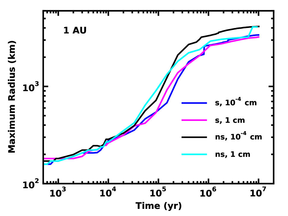
Figure 6: Time evolution of $r_{max}$ the size of the largest object at 1 AU for systems starting with 100 km planetesimals, $r_{min}$ = 1 $\rm\,\mu{\rm m}$ or 1 cm (as labeled), and with (‘s’) or without (‘ns’) stirring from dynamical shake-up. The magnitude of dynamical shake-up and the size of the smallest object in the coagulation grid have little impact on collision outcomes at 1 AU.

At the onset of dynamical shake-up, the migration time scale for Saturn is shorter than for Jupiter. However, a drift time of 2 Myr is still longer than the short disk dissipation time scales considered here. Even if Saturn drifts during the shake-up, the pace and timing of resonance sweep through the asteroid belt and across the orbit of Mars are not expected to change (see Fig. 3). While faster, Type III migration is possible for Saturn when the disk is massive (Masset & Papaloizou, 2003), rapid drift is unlikely when the gas disk surface density is as low as in the scenarios considered here (e.g., Papaloizou et al., 2007, Fig. 6, therein). While migration may be essential for establishing the orbital configuration of Saturn and Jupiter at early times (e.g., Masset & Snellgrove, 2001; Morbidelli & Crida, 2007; Zhang & Zhou, 2010), it is not an important consideration during dynamical shake-up.

Although a lower mass planet may not experience steady inspiral through Type I or Type II migration during dynamical shake-up, it can drift inward if it initially has some eccentricity. As its eccentricity damps, the planet loses energy and drifts radially inward (Adachi et al., 1976; Thommes et al., 2003; Nagasawa et al., 2005). However the drift time is roughly the eccentricity damping time scaled by $e^{-2}$. As long as damping keeps the eccentricity low, radial drift is insignificant. The scenarios considered here have short episodes of eccentricity pumping; radial drift is then small. We confirm this behavior in $n$-body simulations and therefore omit it from consideration. In contrast, Nagasawa et al. (2005) and Thommes et al. (2008) consider models with episodes of eccentricity pumping and damping that last for millions of years. Radial drift is an important feature in those scenarios.

2.2.5 Gas drag

Aerodynamic drag also impacts the orbits of solid particles in the disk (e.g., Chiang & Youdin, 2010). The behavior of solids depends on the mean free path of gas molecules (Adachi et al., 1976; Weidenschilling, 1977a):

$$\lambda_{\rm mfp}\approx\frac{1}{\sigma n_{{\rm gas}}}\approx 100\left[\frac{a}{\textrm{\small 1\,AU}}\right]^{5/4}\left[\frac{\Sigma(a,t)}{\textrm{\small 20\,g/cm${}^{2}$}}\right]^{-1}\left[\frac{h_{0}}{\textrm{\small 0.04\,AU}}\right]\ \textrm{cm},$$ (23)

where $\sigma$ is the cross section of gas molecules, $n_{{\rm gas}}$ is their number density, and the numerical factors in the rightmost expression are suggestive of circumstellar nebula conditions after the gas giants have formed. If particles are comparably sized or smaller than $\lambda_{\rm mfp}$, then molecular collisions dominate the dynamics according to Epstein’s Law. Larger particle sizes or high relative speeds can cause different behavior: Slowly moving particles larger than $\lambda_{\rm mfp}$ experience a viscous force that is proportional to the relative speed — Stoke’s Law. Particles with a radius $r_{{\rm p}}\gg\lambda_{\rm mfp}$ or which have a speed that greatly exceeds the sound speed of the gas produce turbulence and feel a force proportional to the square of the relative speed.

To quantify the importance of gas drag, we consider the stopping time of a particle, defined as

$$t_{\rm stop}\equiv\left|\Delta v/a_{{\rm aero}}\right|,$$ (24)

where $a_{{\rm aero}}$ is the acceleration from aerodynamic drag and $\Delta v$ is the relative speed between the particle and the gas. An astrophysically important value for $\Delta v$ is the difference between the Keplerian orbital speed of a particle, $v_{\rm kep}$, and the circular speed of the gas disk, $v_{\rm gas}$, which is slower because of pressure support. From simple assumptions about the gas pressure (e.g., Youdin & Kenyon, 2013),

$$v_{\rm kep}-v_{\rm gas}\equiv\eta v_{\rm kep},\ \ \ \ \textrm{with}\ \ \ \ \eta\sim(h/a)^{2}\sim 10^{-3},$$ (25)

the “headwind” felt by the particle has a Mach number of

$$\mu=\eta\frac{v_{\rm kep}}{c_{s}}\sim\frac{h}{a}=0.04{\left[\frac{h_{0}}{\textrm{\small 0.04\,AU}}\right]}\left[\frac{a}{\textrm{\small 1\,AU}}\right]^{1/4},$$ (26)

where we have used a sound speed $c_{s}\sim hv_{\rm kep}/a$. With this Mach number and the mean free path in the disk, we can determine the stopping time as a function of particle size.

When the gas density drops to about 1% of its MMSN value, the stopping time becomes comparable to a dynamical time for centimeter-size particles. Just as for meter-size particles at earlier epochs (the ‘meter-size barrier’; Weidenschilling, 1977a; Johansen et al., 2007), these solids cannot become fully entrained in the gas and are doomed to spiral in toward the Sun on a time scale of $\sim 1/\eta$ orbital periods. Under these conditions, smaller dust particles are entrained in the gas. Larger planetesimals are less affected by aerodynamic drag. For example, objects with a size of roughly 10 km are in the turbulent, quadratic regime with stopping times exceeding millions of years.

When the gas is more tenuous and optically thin, the smallest particles dynamically damp, but are then driven away by radiation pressure (Weidenschilling, 1977a; Takeuchi & Artymowicz, 2001). This process plays a key role in planet formation: growing planets stir smaller bodies, triggering a collisional cascade that collisionally grinds debris into dust. The tenuous gas disk and starlight remove material from the small-size tail of the cascade. Thus, there is a mass “drain” for the system that can limit the ultimate size of the planets that drive the cascade (see Kenyon et al., 2016). This phenomenon is the basis for the present work, in which the mass of Mars comes out small because of a collisional cascade driven by dynamical shake-up.

2.3 Secular evolution in the inner solar system

Combining the physics of precession, eccentricity pumping and gas damping, we can track orbits of planetesimals and protoplanets in the inner solar system during the epoch of a sweeping $\nu_{5}$ resonance. From Appendix B, the evolution equations for orbital elements are

$$\frac{de}{dt} = -(\dot{\varpi}_{\rm p}-\dot{\varpi}_{\rm J})e_{\rm force}\sin(\varpi_{s}-\varpi_{J})+e/\tau_{\rm damp},$$ (27)

$$\frac{d\varpi}{dt} = (\dot{\varpi}_{\rm p}-\dot{\varpi}_{\rm J})\left[1-\frac{e_{\rm force}}{e}\cos(\varpi_{s}-\varpi_{J})\right].$$ (28)

We integrate these equations to determine the orbital evolution of a protoplanet, starting from a circular orbit at some early time. We also specify an initial orbital configuration for Jupiter and Saturn, as well as a decay mode for the disk. Our results were validated with numerical simulations based on the $n$-body component of Orchestra with a binned representation of the disk (§2.2.1).

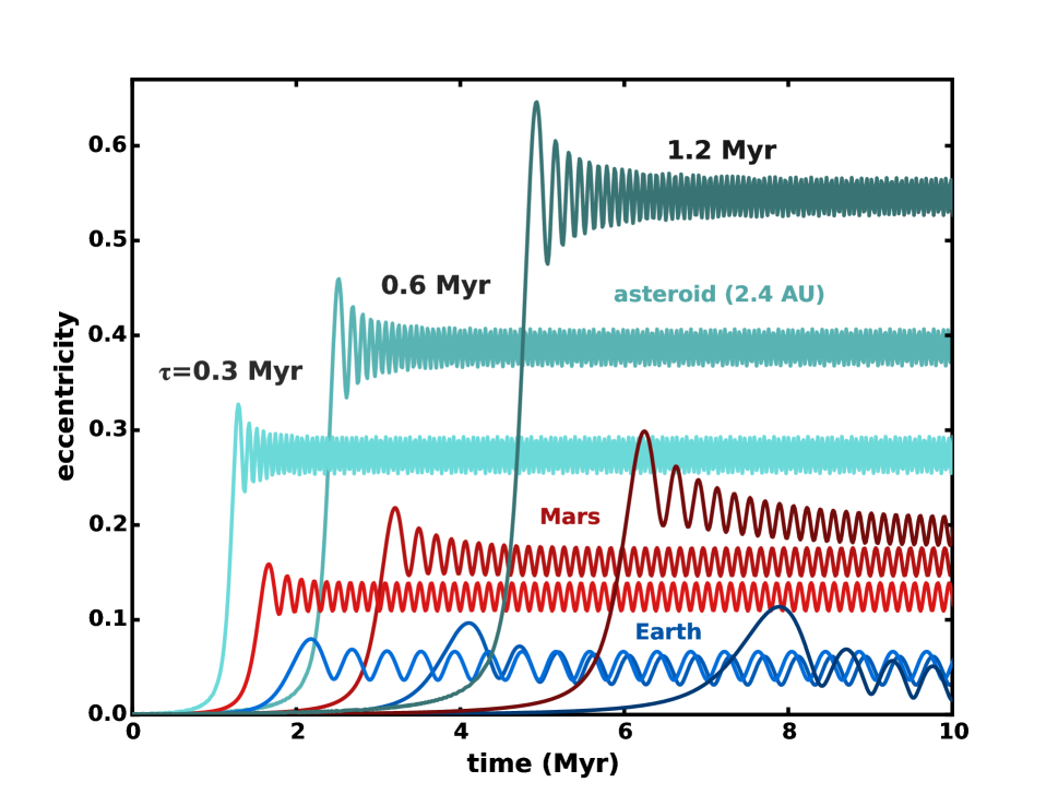
Figure 4: Eccentricity evolution in a gas disk that undergoes uniform depletion. The plot shows the eccentricity of Mars (red curves) and a Ceres-size asteroid at 2.4 AU (cyan curves) as a function of time. The three curves in each set are for different depletion time scales ($\tau$), as labeled (darker is slower depletion). For Mars, some eccentricity damping is apparent, but only for the more slowly decaying disk. With a greater mass, the Earth damps more strongly than Mars and the asteroid. Note that the sweeping resonance hits earlier and with greater effect at larger orbital distance and when the decay of the disk is slow.

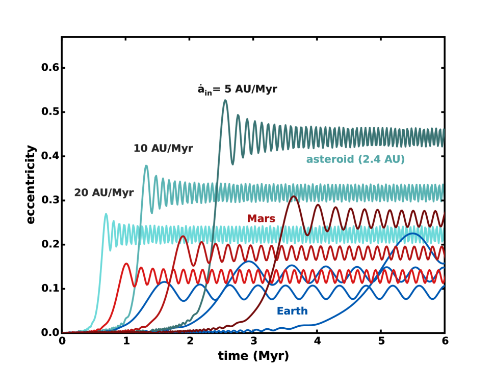
Figure 5: Eccentricity evolution in a disk with an expanding inner edge. As in the previous Figure, the eccentricity of Mars is indicated by the red curves, with darker values corresponding to longer-lived disks (slower ${\dot{a}_{{\rm in}}}$). The curves showing the evolution of a Ceres-like asteroid are in cyan. Slower disk evolution and closer proximity to Jupiter mean more eccentricity pumping. Since the sweeping resonance hits when the disk’s inner edge is well clear of the inner solar system, there is no gas drag in these models.

Figures 4 and 5 show the secular evolution of an Earth-mass planet at 1 AU, Mars at 1.52 AU, and a Ceres-mass asteroid at 2.40 AU in response to Jupiter (5.20 AU) and Saturn (9.58 AU). We assume that only Jupiter contributes to the eccentricity pumping, and we adopt an eccentricity of ${e_{\rm J}}=0.03$, which gives an approximate time-average value as Jupiter’s orbit evolves under the influence of Saturn. To give a sense of the state of the disk when the resonance sweeps inward, the surface density at Mars is 40 g/cm² (compared to an initial $\sim$1300 g/cm²) in the uniform depletion model. In the inside-out erosion scenario, the disk’s inner edge crosses just beyond 15 AU when the resonance hits Mars.

Figures 4 and 5 illustrate that proximity to Jupiter is a key factor in dynamical shake-up (see also Nagasawa et al., 2000, 2005; Thommes et al., 2008). Planetesimals and protoplanets closer to the gas giant experience more eccentricity pumping. The rate of resonance sweeping is also important. Rapidly evolving disks (small $\tau$ or large ${\dot{a}_{{\rm in}}}$) leave protoplanetary orbits less excited. Comparing the final outcomes of the uniform dissipation model and the inside-out clearing scenario, we infer the role of eccentricity damping by gravity wakes (Equation (2.2.4)); the uniform dissipation model has gas in the inner solar system, so objects more massive than Mars orbitally damp by this mechanism. In all other cases involving these short-lived gas disks, orbital damping by gravity wakes is not important.

Although not included in the models described in this section, the inner solar system may have had a long-lived residual disk, replenished by comets or collisions between asteroids (the disk around $\beta$ Pic provides an example; Lagrange et al., 1987; Beust et al., 1996; Czechowski & Mann, 2007; Kral et al., 2016). Even with a low surface density ($\Sigma\ll 10$ g/cm²) this component may help to clear collisional debris during planet formation (Kenyon et al., 2016) and damp eccentricities well after the planets formed. From Equation (2.2.4), we estimate that a residual disk with a surface density of roughly 0.01 g/cm² can damp the orbit of Mars in roughly 1 Gyr.

3 Numerical Simulations

To illustrate the impact of dynamical shake-up on numerical simulations of planet formation, we consider a representative example designed to remove solid material at $a\gtrsim$ 1.5 AU well before protoplanets reach the mass of Mars. From previous simulations of terrestrial planet formation with little dynamical depletion at 1.5–3 AU (e.g., Kenyon & Bromley, 2006; Lunine et al., 2011; Chambers, 2013; Walsh & Levison, 2016; Haghighipour & Winter, 2016), giant impacts produce Mars-mass (Earth-mass) objects in 1–10 Myr (10–100 Myr). Radiometric analyses suggest Mars achieved most of its final mass in $\lesssim$ 3–5 Myr (Dauphas & Chaussidon, 2011; Dauphas & Pourmand, 2011). Thus, we focus on dynamical shake-up scenarios where sweeping secular resonances pass through the terrestrial zone at 1–2 Myr.

Within this scenario, we consider the following sequence of events.

Cloud collapse:

Current models envision formation of a star + disk system during the collapse of a dense core in a giant molecular cloud (McKee & Ostriker, 2007, and references therein). As cloud material falls onto the outer disk, the central protostar and inner disk eject material in a high velocity bipolar jet (e.g., Bontemps et al., 1996; Bally et al., 2007). After roughly 0.5–1 Myr, infall and outflow effectively cease, leaving behind a fairly massive circumstellar disk surrounding a pre-main sequence star (e.g., van Kempen et al., 2009; Eisner, 2012). Radiometric data and the demographics of circumstellar disks suggest formation of 10–100 km or larger planetesimals during this class I phase of evolution (Greaves & Rice, 2010; Dauphas & Chaussidon, 2011; Najita & Kenyon, 2014). In our calculations, the formal $t$ = 0 occurs sometime during the class I phase.

Gas giant formation:

Growth of gas giants is a several step process, involving (i) production of a multi-Earth-mass core of ice and rock, (ii) gradual accumulation of a gaseous atmosphere, and (iii) more rapid accretion of gas from the disk (Pollack et al., 1996; Pierens & Nelson, 2013; Piso & Youdin, 2014). We assume that Jupiter and Saturn grow quickly out of icy planetesimals on a time scale of $\tau_{f}\approx$ 0.5–1 Myr (Kenyon & Bromley, 2009; Bromley & Kenyon, 2011; Levison et al., 2015; Chambers, 2016). The nominal formation time is sensitive to the mode of disk dispersal: gas giants need to form more rapidly in disks dissipating from the inside-out than in disks depleting homologously with radius. Depending on conditions within the disk, cores may migrate as they grow (see, e.g., Paardekooper & Mellema, 2006; Lyra et al., 2010; Cossou et al., 2014; Bitsch et al., 2015).

Disk dissipation:

Disk depletion occurs in parallel with the growth of gas giant planets. For simplicity, we adopt a uniform depletion model with $\tau=0.3$ Myr. Dynamical shake-up with inside-out depletion at ${\dot{a}_{{\rm in}}}=20$ AU/Myr has a similar impact on the growth of solids at 1.5–3 AU. The major difference between the two scenarios is the amount of residual gas available to clear collisional debris in the terrestrial zone.

Gas giant migration:

Once gas giants reach a critical mass, they open up a gap and begin to migrate through the disk. When $\tau_{f}\ll\tau$, migration is ubiquitous (e.g., Walsh et al., 2011). If $\tau_{f}\gtrsim\tau$, however, the smaller surface densities in the disk lead to longer drift time scales (Equation (22)). Gas giants then may be unable to migrate far once they approach their final masses.

Resonance sweeping:

As the disk depletes, resonant excitations sweep through the terrestrial zone. Material closest to the giant planets experience resonances before material closer to the Sun (Figure 2). In contrast, growth of solids is faster closer to the Sun. Thus, growth is limited most (least) severely in the asteroid belt (inside 1 AU). Depending on the level of gas depletion, aerodynamic drag may remove collision fragments with sizes of 1 cm and smaller (see also Kenyon et al., 2016).

In our approach, Jupiter and Saturn reach their final masses rapidly and are in place when resonance sweeping begins. These assumptions are reasonable for (i) systems with $\tau_{f}\ll\tau$, where the gas giants finish any migration through the gas (including a Grand Tack) prior to significant disk depletion and (ii) systems with $\tau_{f}\approx\tau$, where the surface density of the disk is too small to support much radial migration. We further assume that any migration of the gas giants has a negligible impact on the surface density of solids, which allows us to compare the depletion that might be produced by migration (Walsh et al., 2011; Batygin & Laughlin, 2015) with the depletion due to resonance sweeping.

To follow the evolution of solids in the terrestrial zone, we perform a coagulation calculation (Safronov, 1969; Spaute et al., 1991; Kenyon & Luu, 1998; Ohtsuki et al., 2002; Kenyon & Bromley, 2006, 2008). In our approach, described in Appendix C, we seed 32 concentric annuli with a swarm of 1–100 km planetesimals having $\Sigma_{s}\propto a^{-3/2}$ over 1–3 AU. Within each annulus, we track the mass and velocity evolution of particles with sizes ranging from a minimum size $r_{min}$ to a maximum size $r_{max}$. For improved accuracy, the mass spacing factor between adjacent bins is $\delta=2^{1/4}$. Using well-tested statistical techniques, the code calculates the outcomes of gravitational scattering and physical collisions among all mass bins in all annuli. The appendix describes the algorithms in more detail.

For this study, we add a mechanism for eccentricity pumping from Jupiter during the phase of the sweeping secular resonance:

$$\dot{e}=\begin{cases}\frac{1}{\sqrt{2}}{\dot{e}_{{\rm pump}}}&\ \ \ \textrm{if $(e<\sqrt{2}e_{\rm force})$}\\ 0&\ \ \ \textrm{otherwise.}\end{cases}$$ (29)

This algorithm works well in reproducing the eccentricity pumping in numerical experiments using secular perturbation theory and the $n$-body component of Orchestra. In the presence of a dissipating gas disk, we apply this algorithm at all times. If the disk is static or absent altogether, we turn off this stirring.

For this calculation, we consider a mono-disperse set of solid planetesimals with initial radius $R_{0}$ = 100 km and total mass $M_{0}$. The planetesimals have mass density $\rho_{{\rm p}}$ = 3 $\rm g~{}cm^{-3}$, initial eccentricity $e_{0}=10^{-3}$, and initial inclination $\imath_{0}=e/2$. We consider grids extending from 1 AU to 3 AU with $r_{min}$ = 1 $\rm\,\mu{\rm m}$ or 1 cm. For simplicity, we neglect gas drag. Throughout the evolution we consider, collisional damping, dynamical friction, and viscous stirring dominate reduction of small particle velocities by gas drag (e.g., Wetherill & Stewart, 1993; Kenyon & Luu, 1998). However, the gas can still generate a substantial radial drift, which removes small particles from the grid (e.g., Kenyon et al., 2016). Adopting two different values for $r_{min}$ allows us to quantify the potential importance of radial drift without spending extra cpu time on a more complicated calculation. Here our goal is to learn whether dynamical shake-up can prevent the growth of protoplanets inside of 3 AU. In a more realistic system, gas drag probably aids planet growth at the inner edge of the grid and prevents growth at the outer edge.

4 Results

In calculations with no sweeping resonance, growth follows a standard pattern. Collisions among 100 km planetesimals with $e_{0}=10^{-3}$ produce mergers and some debris. As the largest objects grow, dynamical friction damps their orbits. Damping leads to larger gravitational focusing factors and a short phase of runaway growth when protoplanets reach radii of 1000-2000 km. During runaway growth, viscous stirring excites the orbits of leftover planetesimals and smaller particles of debris. Stirring initiates a collisional cascade which grinds leftovers into smaller and smaller particles that are ejected by radiation pressure. Loss of material slows the growth of protoplanets, which reach a characteristic maximum size of 3000 km.

When the resonance sweeps through the grid, it tends to drive all of the solids to large $e$ (e.g., Figure 4). Among the solids, dynamical friction tries to damp $e$ and $i$ of the largest protoplanets. When the resonance is strong (weak), dynamical friction cannot (can) keep up with resonant stirring. Thus, strong resonances drive a collisional cascade before protoplanets have a chance to grow.

Figure 6 illustrates the evolution of the largest objects at 1 AU in four separate simulations. Early on, 100 km objects collide and merge into larger objects. After $1-2\times 10^{4}$ yr, the largest objects reach 300 km sizes. By $10^{5}$ yr, mergers have produced a set of 500–600 km objects. After $10^{5}$ yr, the largest objects in the simulations follow similar but somewhat divergent tracks. Fairly independent of $r_{min}$, systems with no dynamical stirring (labeled ‘ns’ in the Figure) grow somewhat faster than systems with dynamical stirring (labeled ‘s’). After 10 Myr, the largest objects in the ‘ns’ (‘s’) tracks reach sizes of 4000 km (3000 km).

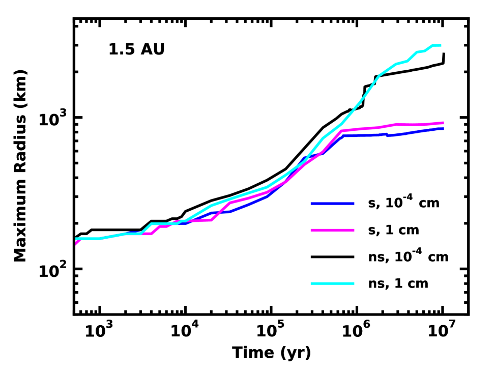
Figure 7: As in Figure 6 for calculations at 1.5 AU. Collision outcomes do not depend on $r_{min}$(values are listed in the legend); however, dynamical shake-up (’s’) reduces $r_{max}$ by factors of 3–5 on time scales of 1–10 Myr as compared with no dynamical stirring (’ns’).

At 1.5 AU, the differences in the evolution are more dramatic (Figure 7). As in systems of planetesimals at 1 AU, the evolution for 0.1–0.3 Myr is independent of $r_{min}$ or the level of stirring. By 1 Myr, slower growth in systems with dynamical stirring is evident. After 10 Myr, systems with (without) stirring have objects with maximum sizes of 800–1000 km (2000–3000 km). Independent of stirring, the maximum size is insensitive to $r_{min}$.

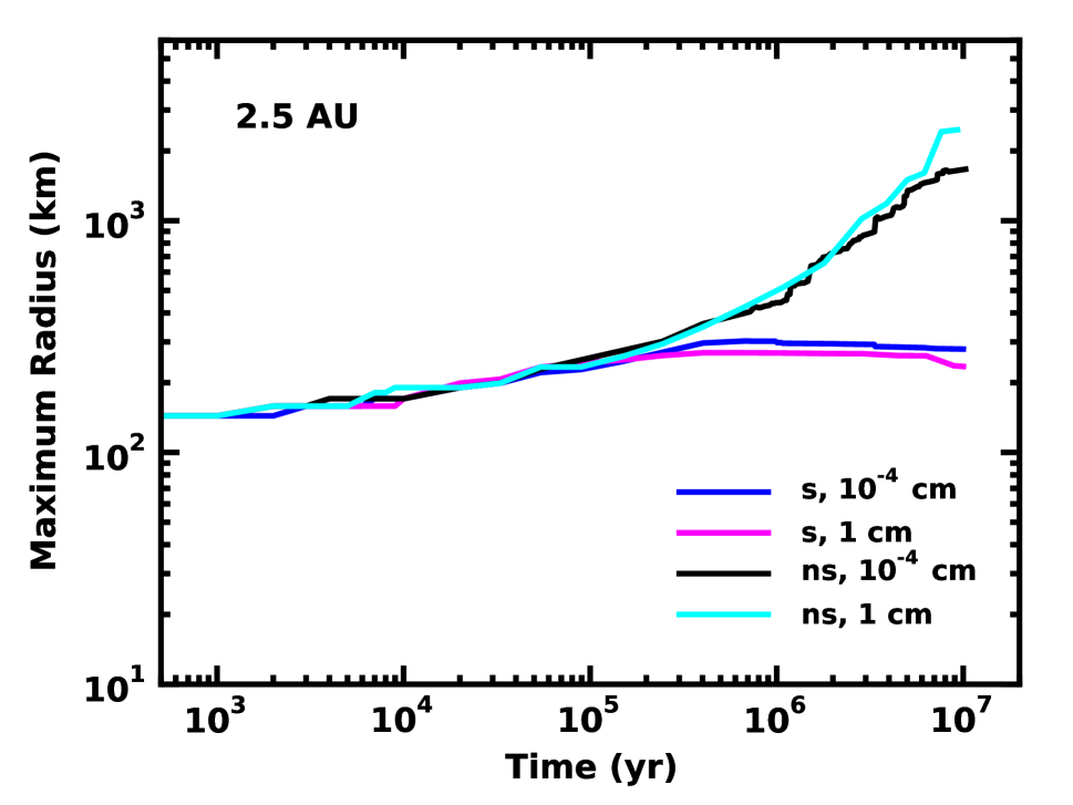
Figure 8: As in Figure 6 for calculations at 2.5 AU. Dynamical shake-up (’s’; $r_{min}$ values are shown) reduces $r_{max}$ by factors of 10, compared to calculations with no stirring (’ns’).

At 2.5 AU, dynamical stirring prevents large objects from growing past 200–300 km (Figure 8). After 0.1–0.3 Myr of growth, the largest objects reach typical maximum sizes of 300 km. In models with no dynamical stirring, the largest objects grow slowly to 500 km sizes at 1 Myr and 2000 km sizes at 10 Myr. In models with dynamical stirring, however, growth effectively ceases once stirring begins. As the evolution proceeds, high velocity collisions with small objects gradually diminish the sizes of the largest objects. After reaching peak sizes of 300 km at roughly 1 Myr, the largest objects have radii of roughly 200 km after 10–100 Myr.

In this example, collisional cascades driven solely by dynamical shake-up remove a large fraction of solid material from the system. When $r_{min}$ = 1 $\rm\,\mu{\rm m}$ (1 cm), systems with dynamical shake-up lose 30% (95%) of their initial mass in solids. In models without dynamical shake-up, mass loss by collisional disruption is much less severe, $\lesssim$ 5% when $r_{min}$ = 1 $\rm\,\mu{\rm m}$ and 60% when $r_{min}$ = 1 cm.

These results demonstrate that sweeping secular resonances have a profound influence on the outcomes of terrestrial planet formation inside the orbit of Jupiter (see also Thommes et al., 2008). For the initial conditions examined here, there is little impact on planet formation inside 1 AU: planet formation is fairly rapid and dynamical shake-up is rather weak. At larger $a$ where the resonance is much stronger, the growth of planets is much slower. At 1.5 AU, protoplanet growth stalls at 1000 km. At 2.5 AU, protoplanets barely grow larger than 300 km.

The models considered here assume that Saturn orbits at its current position. Unless Saturn is closer than the 3:2 orbital commensurability with Jupiter, relaxing this assumption does not change our results significantly. In compact configurations, the $\nu_{5}$ resonance crosses just inside of Mars’ orbit and fails to reach 1 AU (Fig. 3). Dynamical excitation may then completely clear a narrow region between Earth and Mars, without stirring Earth’s progenitors at all. Moving both gas giants to larger orbital distance, decreasing their separation, or both, can prevent the sweeping resonance from reaching Mars. Moving both giants closer can destructively stir material even at Earth’s location. Thus, the orbits and masses of Earth and Mars provide constraints on the history gas giant’s orbital configuration (see Brasser et al., 2009; Minton & Malhotra, 2011; Agnor & Lin, 2012; Kaib & Chambers, 2016; Haghighipour & Winter, 2016).

5 Implications for exoplanetary systems

Dynamical shake-up is likely to occur around stars other than the Sun. We expect sweeping resonances within circumstellar disks in stellar binaries (e.g., Heppenheimer, 1978; Kley & Nelson, 2008; Paardekooper et al., 2008; Rafikov, 2013) and in circumbinary disks (e.g., Marzari et al., 2008; Silsbee & Rafikov, 2015). For star-planet binaries like the Sun and Jupiter, and for regions interior to the giant planet, we can use Equation (16) for eccentricity pumping to estimate under what conditions a dynamical shake-up is important. By multiplying the pumping rate and the gas disk life-time, we find

$$e_{\rm bin}\,\mu_{\rm bin}\,\left(\frac{T_{\rm gas}}{T_{\rm bin}}\right)\left(\frac{T}{T_{\rm bin}}\right)^{\!5/3}\ \gtrsim\ 0.1\,,$$ (30)

where $e_{\rm bin}$ is the binary eccentricity, $\mu_{\rm bin}$ is the giant planet’s mass relative to the host star, $T_{\rm bin}$ is its orbital period, $T_{\rm gas}$ characterizes the gas disk life time, and $T$ is an interior body’s Keplerian orbital period. For Earth’s location in the Sun-Jupiter binary, and with $T_{\rm gas}$ set to $10^{6}$ yr, the left-hand side of the expression is roughly 0.05, suggesting that dynamical shake-up is not important. On the other hand, the left-hand side exceeds the threshold value of 0.1 for both Mars at 1.5 AU and an asteroid at 2.5 AU, with values of 0.13 and 0.45, respectively.

Stars with a massive planet near or beyond the snow line are fairly common. Radial velocity surveys (Bonfils et al., 2011) and microlensing studies (Shvartzvald et al., 2016) suggest that as many as 50% of M dwarfs host icy super-Earths, and up to 5% host Jupiter-mass planets. Eccentricity estimates of all known long-period exoplanets are consistent with $e\gtrsim 0.02$ (Han et al., 2014). Equation (30) suggests that even super-Earths can cause a shake-up, when (i) the mass of the host star is low, (ii) the gas dissipation time scale is long, and/or (iii) the eccentricity of the massive planet is large. Thus, scaled-down versions of asteroid belts around M dwarfs are plausible.

Unless the star’s disk dissipates slowly or the planet’s orbit is strongly eccentric, a Sun-like star requires a Jupiter-mass planet for shake-up. Radial velocity studies suggest that 5–10% of Sun-like stars host gas giants out to 5 AU (Cumming et al., 2008; Zechmeister et al., 2013). Consistent with theory (Kennedy & Kenyon, 2008), more massive (A- and F-type) stars show a slight increase in the frequency of giant planets (Lovis & Mayor, 2007; Johnson et al., 2007; Bowler et al., 2010). While most of the observed giant planets have shorter orbital periods than the Sun-Jupiter binary, they still admit the possibility of an extended region in the terrestrial zone that experienced dynamical shake-up. We conclude that asteroid belt analogs may be found interior to the gas giants in a broad range of stellar hosts.

From our sample calculations of dynamical shake-up, planetary systems that experience a sweeping resonance have an early, enhanced production of dusty debris compared to systems with no outer gas giant. In systems where the gas has negligible surface density, copious dust production is probably visible (e.g., Kenyon & Bromley, 2004b, 2016). If the disk has a modest surface density of 0.01–20 g cm^-2 during the shake-up, however, collisional debris is probably cleared out rapidly by gas drag and radiation pressure (Weidenschilling, 1977a; Takeuchi & Artymowicz, 2001). In these systems, rocky planet formation may be “quick” and “neat” (Kenyon et al., 2016).

6 Summary

In this paper, we describe a scenario for rocky planet formation that includes a sweeping secular resonance driven by Jupiter and the dissipating solar nebula. As in the dynamical shake-up models proposed in previous work (Nagasawa et al., 2005, 2007; O’Brien et al., 2007; Thommes et al., 2008), we try to explain the low mass of Mars and the asteroid belt. Our new contribution is to explore outcomes when the resonance sweeps through the inner solar system quickly, before the formation of Mars is complete. This key modification allows Jupiter’s eccentricity pumping to increase fragmentation from high velocity collisions during the runaway and oligarchic phases of planet formation. Coupled with clearing of small debris particles by gas drag and radiation pressure, this process yields a way to inhibit the growth of protoplanets beyond 1 AU.

Our coagulation calculations with the Orchestra code illustrate that an early sweep of the $\nu_{5}$ secular resonance explains the low mass of Mars, as well as the sizes of objects and total mass in the asteroid belt. We ran two extensive multi-annulus coagulation simulations, with and without a sweeping resonance. As in other simulations of planet formation within the terrestrial zone (e.g., Chambers, 2001; O’Brien et al., 2006; Kenyon & Bromley, 2006; Raymond et al., 2009; Morishima et al., 2010), calculations without the resonance yielded Earth-size protoplanets on a Myr time scale. In contrast, calculations with the sweeping resonance produce protoplanets that reach only $10^{3}$ km in a significantly depleted disk.

Models with a dynamical shake-up at later times, with disk dissipation time scales of 5–10 Myr, successfully limit the mass of Mars and clear the asteroid belt (e.g., Nagasawa et al., 2007). In these scenarios, orbital energy losses of solids in a more slowly sweeping resonance and a longer-lived gas disk become important, and material drifts radially inward. The building blocks of the rocky planets then originate as far way as the asteroid belt and migrate inward with the resonance. The formation time for Mars in these scenarios exceeds 10 Myr, consistent with available radiometric data at the time (Jacobsen, 2005). Our version of the shake-up scenario with in situ formation is motivated by more recent evidence for a shorter formation time for Mars (Dauphas & Pourmand, 2011).

In dynamical shake-up scenarios like those discussed here, Jupiter is in place near its present orbital distance. While we also choose Saturn’s orbit to be similar to its present-day configuration, a shake-up will occur at Mars’ location and in the asteroid belt even if Saturn is near the 3:2 commensurability, around 7 AU. Thus, dynamical shake-up may occur as a precursor to late-time orbital instability scenarios like the Nice model (Tsiganis et al., 2005), which requires Saturn’s to orbit closer to Jupiter than it is now.

Jupiter’s orbital eccentricity is key to dynamical shake-up. If the gas giant was assembled close to its current location, as in “classical” models (see Haghighipour & Winter, 2016, and references therein), interactions with the gas disk produce a large enough eccentricity to drive a shake-up (Goldreich & Sari, 2003; Duffell & Chiang, 2015). In other scenarios, convergent migration leads to resonance trapping between Jupiter and Saturn (Masset & Snellgrove, 2001; Morbidelli & Crida, 2007). The Grand Tack (Walsh et al., 2011) is one example, tuned to trigger the resonance trap and mutual outward drift only after the gas giants are deep inside the terrestrial zone. Jupiter’s eccentricity in these models may have been low (e.g., Morbidelli et al., 2007; Deienno et al., 2016). However, 2D hydrodynamical calculations suggest that with Jupiter and Saturn in a 2:1 mean-motion resonance (a configuration favored in the Nice model; Nesvorný & Morbidelli, 2012), Jupiter’s eccentricity is ${e_{\rm J}}\approx 0.03$ (Pierens et al., 2014), as in our shake-up models. There is also evidence from 3D simulations that ${e_{\rm J}}$ can grow to this level when Jupiter and Saturn occupy the 3:2 resonance (D’Angelo & Marzari, 2012). Thus, conditions for dynamical shake-up arise in a variety of scenarios.

As a constraint for planet formation theory, the mass of Mars is a challenge (Wetherill, 1991). Models allow a range of possibilities, including an initially truncated protoplanetary disk at 1 AU (Jin et al., 2008; Hansen, 2009; Izidoro et al., 2014; Haghighipour & Winter, 2016), dynamical excitation and depletion (Wetherill, 1992; Raymond et al., 2009), and the Grand Tack (Walsh et al., 2011). Compared to these scenarios, a dynamical shake-up has a clear advantage: a sweeping resonance generated by the dissipation of a disk where the gas giants formed seems inevitable. Our work here suggests that this phenomenon alone can explain the low mass of Mars and a depleted asteroid belt.

As these theoretical scenarios become more complete, it should become possible to predict the formation time scale of Mars, $\tau_{f}$, as well as the dynamical architecture of Mars and the asteroid belt as functions of $\tau_{f}$ and the gas disk lifetime, $\tau$. We expect that systems with $\tau_{f}\ll\tau$ will be prone to depletion from Grand Tack and dynamical shake-up; systems with longer $\tau_{f}$ may only undergo dynamical shake-up. If this hypothesis is correct, disks with longer $\tau_{f}$ may yield more massive analogs of Mars and the asteroid belt than those with smaller $\tau_{f}$. As observational constraints on $\tau$ and $\tau_{f}$ improve (e.g., Dauphas & Chaussidon, 2011; Connelly et al., 2012; Tang & Dauphas, 2014; Morris et al., 2015; Schiller et al., 2015; Dauphas, 2017; Fischer-Gödde & Kleine, 2017; Wang et al., 2017), it will be possible to test this prediction.

Our models have several connections to observations of exoplanetary systems. If dynamical shake-up is inevitable for a planetary system with a long-period giant planet, asteroid belt analogs should be as common as gas giant planets. Roughly 10% of Sun-like stars with Jupiter-mass planets and a higher fraction of M dwarfs with super-Earths and Neptunes are configured in this way. Assuming an initially massive disk of solids between the super-Earth/gas giant and the central star, Mars analogs and extrasolar asteroid belts should be similarly frequent. Future exoplanet searches may detect these planets directly from transits (e.g., Borucki et al., 2013), while sensitive microlensing surveys may reveal extrasolar asteroid belts (Lake et al., 2017).

Observations of young planetary systems may reveal dynamical shake-up in action, since a large amount of debris is produced compared to systems without a shake-up. Detection of this debris depends on the timing of resonance sweeping and the manner of disk depletion. Unless the gas drags solid material into the central star (Kenyon et al., 2016), we expect brighter dust signatures in transition disk systems with gas giant planets at 5–10 AU than in those without gas giants.

The results of this preliminary study are promising. In future work we will include a more accurate treatment of the dynamics within Orchestra’s $n$-body code. Then we can begin to compare the final outcomes of an early dynamical shake-up with the observed orbits of the Sun’s asteroids. We also plan to include more detailed modeling of the small debris from collisions. Our assumptions here are that this debris is rapidly cleared from the terrestrial zone, making its detection in this region difficult (cf. Kenyon & Bromley, 2004b). If this idea is true, it would explain the low incidence of debris disks in the terrestrial zones of other stars (e.g., Mamajek et al., 2004) while still offering hope that these stars host planets like Earth.

Appendix A Theory of circumstellar orbits in a binary system

Here we derive analytical expressions that describe the orbit of a small body, such as an isolated planetesimal or protoplanet, in a binary system. Taking the approach of Lee & Peale (2006) and Leung & Lee (2013) for circumbinary orbits, our starting point is the restricted three-body problem (see Szebehely, 1967; Murray & Dermott, 1999). The primary and secondary have masses $M_{1}$ and $M_{2}$, respectively; the binary has separation ${a_{\rm bin}}$ and eccentricity $e_{\rm bin}$. To quantify positions and velocities, we choose a cylindrical coordinate system with the binary at zero altitude ($z=0$) and an origin located on the primary or the binary’s center of mass, depending on whether we are interested in circumbinary (P-type) or “intrabinary” (S-type) orbits. In the intrabinary case, we take the “primary” to mean the star that hosts the planetesimal or protoplanet in question. The theory presented below holds even if the “secondary” is more massive than the primary.

The gravitational potential at the position $(R,\phi,z)$ of a small body on an intrabinary orbit is

$$\Phi=-\frac{GM_{1}}{\sqrt{R^{2}+z^{2}+R_{1}^{2}+2RR_{1}\cos\Delta\phi}}-\frac{GM_{2}}{\sqrt{R^{2}+z^{2}+R_{2}^{2}-2RR_{2}\cos\Delta\phi}},$$ (A1)

where $R_{1}$ ($R_{2}$) is the distance from the origin to the primary (secondary), $G$ is the gravitational constant, and $\Delta\phi$ is the small body’s position angle relative to the direction of the secondary. The gradient of this potential contributes to the small object’s equations of motion, from which we obtain orbit solutions by following Lee & Peale (2006) and Leung & Lee (2013): We first express the potential as a cosine series, taken to first order in the binary eccentricity. Then, we adopt a coordinate system that describes the small body’s position and velocity relative to a circular guiding center, and linearize the equations of motion in these coordinates. This strategy allow orbits to be solved in the manner of a driven harmonic oscillator. Lee & Peale (2006) and Leung & Lee (2013) provide details, along the lines of these instructions:

1. Create a series expansion of the potential, first in terms of powers of angle cosines, then rewritten with harmonics:

   $$\Phi=\sum_{k=0}^{\infty}P_{k}\cos^{k}(\Delta\phi)=\sum_{k=0}^{\infty}P^{\prime}_{k}\cos(k\Delta\phi),$$ (A2)

   using multiple angle formulae. For the intrabinary case, we set the coordinate origin to be coincident with the primary, and we modify the potential to account for this choice of a non-inertial frame:

   $$\Phi\rightarrow\Phi+\frac{GM_{2}R}{R_{2}^{2}}\cos(\Delta\phi).$$ (A3)

   The new term compensates for the motion of the primary in the equations of motion.

2. Include the dependence on binary eccentricity by writing

   $$R_{2}/{a_{\rm bin}}\approx 1-e_{\rm bin}\cos{\Omega_{\rm bin}}t,$$ (A4)

   and

   $$\Delta\phi=\phi-\phi_{2}\approx{\Omega_{\rm bin}}t+2e_{\rm bin}\sin{\Omega_{\rm bin}}t$$ (A5)

   where $\phi_{2}$ is the azimuthal coordinate of the secondary, ${\Omega_{\rm bin}}$ is the binary’s mean motion, and time $t$ is chosen to place the binary at periapse when $t=0$ and $\phi_{2}=0$. In the circumbinary case, Equation (A4), along with one like it for $R_{1}$, includes a mass ratio factor to account for center-of-mass coordinates (see Leung & Lee, 2013).

3. Expand the potential to first order in $e_{\rm bin}$ with the form

   $$\Phi(z=0) = \sum_{k=0}^{\infty}\left[\Phi_{k}-e_{\rm bin}\cos({\Omega_{\rm bin}}t)\Phi^{e}_{k}\right]\cos(k\Delta\phi)$$ (A6)

   $$= \sum_{k=0}^{\infty}\Bigg{\{}\Phi_{k}\cos k(\phi-{\Omega_{\rm bin}}t)+$$

   $$e_{\rm bin}\bigg{[}\left(k\Phi_{k}-\text@frac{1}{2}\Phi^{e}_{k}\right)\cos(k\phi-(k+1){\Omega_{\rm bin}}t)+$$

   $$\ \ \ \ \,\left(-k\Phi_{k}-\text@frac{1}{2}\Phi^{e}_{k}\right)\cos(k\phi-(k-1){\Omega_{\rm bin}}t)\bigg{]}\Bigg{\}}$$

   where the upper equation defines $\Phi_{k}$ and $\Phi^{e}_{k}$ (following the convention of Leung & Lee 2013) as expansion coefficients when we take into account the dependence on $e_{\rm bin}$ in the binary’s radial position ($R_{1}$ and $R_{2}$, as in Equation (A4)) but not in the angular coordinates $k\Delta\phi$. The lower equation, which shows full first-order dependence on $e_{\rm bin}$, takes advantage of multiple angle formulae and a Taylor expansion of $\cos\Delta\phi$ to express the potential as a cosine series. Here we limit our analysis to the plane of the binary.

4. Solve equations of motion, including

   $$\ddot{R}-R\dot{\phi}^{2}=-\frac{\partial\Phi}{\partial R}\ \ \ \ \ \textrm{and}\ \ \ \ \ R\ddot{\phi}+2\dot{R}\dot{\phi}=-\frac{1}{R}\frac{\partial\Phi}{\partial\phi},$$ (A8)

   in terms of variables ${R_{\rm g}}+R_{1}$, and ${\Omega_{\rm g}}t+\phi_{1}$, where ${R_{\rm g}}$ is the orbital radius of a guiding center on a circular path about the primary (or center of mass, in the circumbinary case), and ${\Omega_{\rm g}}$ is the mean motion at that orbital distance, given by

   $${\Omega_{\rm g}}^{2}=\frac{1}{{R_{\rm g}}}\left.\frac{d\Phi_{0}}{dR}\right|_{R_{\rm g}}.$$ (A9)

   Keeping only terms that are linear in variables $R_{1}$ and $\phi_{1}$, use the approximation of $\Phi$ as a sum of harmonic modes. The equations of motion and their solutions are the same as in a simple, driven harmonic oscillator; solutions to $R$, $\phi$ (and $z$, it turns out) will also be sums of these same modes.

These steps, with straightforward modification to include motion in the $z$ direction (out of the binary’s orbital plane), lead to these solutions:

$$R(t) = {R_{\rm g}}\left\{1-e_{\rm free}\cos(\kappa_{\rm e}t+\psi_{e})\ -\sum_{k=1}^{\infty}{C_{k}}\cos(k(\omega_{\rm rel}+{\gamma})t)\right.$$

$$\left.-e_{\rm bin}\left[{\tilde{C}}^{e}_{0}\cos({\Omega_{\rm bin}}t+\psi_{\rm bin})+\sum_{k=1}^{\infty}{\tilde{C}}^{+}_{k}\cos(k(\omega_{\rm rel}-{\Omega_{\rm bin}}+{\gamma})t-\psi_{\rm bin})\right.\right.$$

$$\left.\left.\ \ \ \ \ \ \ \ \ \ \ \ \ \ \ \ \ \ \ \ \ \ \ \ \ \ \ \ \ \ \ \ \ \ \ +\sum_{k=1}^{\infty}{\tilde{C}}^{-}_{k}\cos(k(\omega_{\rm rel}+{\Omega_{\rm bin}}+{\gamma})t+\psi_{\rm bin})\right]\right\}$$

$$\phi(t) = {\Omega_{\rm g}}\left\{t+\frac{2e_{\rm free}}{\kappa_{\rm e}}\sin(\kappa_{\rm e}t+\psi_{e})\ \ +\sum_{k=1}^{\infty}\frac{D_{k}}{k\omega_{\rm rel}}\sin(k(\omega_{\rm rel}+{\gamma})t)\right.$$

$$\left.+e_{\rm bin}\left[\frac{{\tilde{D}}^{e}_{0}}{{\Omega_{\rm bin}}}\sin({\Omega_{\rm bin}}t+\psi_{\rm bin})+\sum_{k=1}^{\infty}\frac{{\tilde{D}}^{+}_{k}\sin(k(\omega_{\rm rel}-{\Omega_{\rm bin}}+{\gamma})t-\psi_{\rm bin})}{k\omega_{\rm rel}-{\Omega_{\rm bin}}}\right.\right.$$

$$\left.\left.\ \ \ \ \ \ \ \ \ \ \ \ \ \ \ \ \ \ \ \ \ \ \ \ \ \ \ \ \ \ \ \ \ \ \ \ \ +\sum_{k=1}^{\infty}\frac{{\tilde{D}}^{-}_{k}\sin(k(\omega_{\rm rel}+{\Omega_{\rm bin}}+{\gamma})t+\psi_{\rm bin})}{k\omega_{\rm rel}+{\Omega_{\rm bin}}}\right]\right\}$$

$$z(t)=i{R_{\rm g}}\cos(\kappa_{\rm i}t+\psi_{i}),\hskip 271.0125pt$$ (A12)

where $\omega_{\rm rel}\equiv{\Omega_{\rm g}}-{\Omega_{\rm bin}}$ (a negative value indicates a circumbinary orbit), $e_{\rm free}$ is the “free” eccentricity, $i$ is the inclination, ${\gamma}\equiv{\psi_{\rm g}}-\psi_{\rm bin}-\varpi_{\rm bin}$, where $\varpi_{\rm bin}$ is the binary’s longitude of periastron, and the phase angles ${\psi_{\rm g}}$, $\psi_{\rm bin}$, $\psi_{e}$ and $\psi_{i}$ are constants. The epicyclic frequencies that appear in these solutions are

$$\kappa_{\rm e}^{2}\equiv{R_{\rm g}}\left.\frac{d{\Omega_{\rm g}}^{2}}{dR}\right|_{R_{\rm g}}\!\!+4{\Omega_{\rm g}}^{2}\ \ \ \ \ \textrm{and}\ \ \ \ \ \kappa_{\rm i}^{2}\equiv\left.\frac{1}{z}\frac{d\Phi}{dz}\right|_{z=0,{R_{\rm g}}},$$ (A13)

while the mode amplitudes are

$$C_{k} = \frac{1}{{R_{\rm g}}(\kappa_{\rm e}^{2}-k^{2}\omega_{\rm rel}^{2})}\left[\frac{d\Phi_{k}}{dR}+\frac{2{\Omega_{\rm g}}\Phi_{k}}{{R_{\rm g}}\omega_{\rm rel}}\right]_{{R_{\rm g}}},$$ (A14)

$${\tilde{C}}^{e}_{0} = -\frac{1}{{R_{\rm g}}(\kappa_{\rm e}^{2}-{\Omega_{\rm bin}}^{2})}\left[\frac{d\Phi^{e}_{0}}{dR}\right]_{{R_{\rm g}}},$$ (A15)

$${\tilde{C}}^{\pm}_{k} = \frac{1}{R[\kappa_{\rm e}^{2}-(k\omega_{\rm rel}\pm{\Omega_{\rm bin}})^{2}]}\left[\pm k\frac{d\Phi_{k}}{dR}-\frac{1}{2}\frac{d\Phi^{e}_{k}}{dR}+\frac{k{\Omega_{\rm g}}(\pm 2k\Phi_{k}-\Phi^{e}_{k})}{R(k\omega_{\rm rel}\pm{\Omega_{\rm bin}})}\right]_{{R_{\rm g}}},$$ (A16)

and

$$D_{k} = 2C_{k}-\left[\frac{\Phi_{k}}{{R_{\rm g}}^{2}{\Omega_{\rm g}}\omega_{\rm rel}}\right]_{{R_{\rm g}}},$$ (A17)

$${\tilde{D}}^{e}_{0} = 2{\tilde{C}}^{e}_{0},$$ (A18)

$${\tilde{D}}^{\pm}_{k} = 2{\tilde{C}}^{\pm}_{k}-\left[\frac{k(\pm 2k\Phi_{k}-\Phi^{e}_{k})}{2{R_{\rm g}}^{2}{\Omega_{\rm g}}(k\omega_{\rm rel}\pm{\Omega_{\rm bin}})}\right]_{{R_{\rm g}}}$$ (A19)

(Equations (28–30) and (32–34) in Leung & Lee, 2013).

To complete the problem, we need only calculate the coefficients $\Phi_{k}$ and $\Phi^{e}_{k}$ from Taylor expansions of the full potential, $\Phi$. For the circumbinary case, the expansion variable is ${a_{\rm bin}}/{R_{\rm g}}$, while for an intrabinary orbit, we use ${R_{\rm g}}/{a_{\rm bin}}$. For example, in the intrabinary configuration, the first few coefficients are

$$\Phi_{0} = -\frac{GM_{1}}{{R_{\rm g}}}-\frac{GM_{2}}{{a_{\rm bin}}}\left(1+\frac{1}{4}\frac{{R_{\rm g}}^{2}}{{a_{\rm bin}}^{2}}+\frac{9}{64}\frac{{R_{\rm g}}^{4}}{{a_{\rm bin}}^{4}}+\frac{25}{256}\frac{{R_{\rm g}}^{6}}{{a_{\rm bin}}^{6}}+\dots\right),$$ (A20)

$$\Phi_{1} = -\frac{GM_{2}}{{a_{\rm bin}}}\left(\frac{3}{8}\frac{{R_{\rm g}}^{3}}{{a_{\rm bin}}^{3}}+\frac{15}{64}\frac{{R_{\rm g}}^{5}}{{a_{\rm bin}}^{5}}+\dots\right),$$ (A21)

$$\Phi_{2} = -\frac{GM_{2}}{{a_{\rm bin}}}\left(\frac{3}{4}\frac{{R_{\rm g}}^{2}}{{a_{\rm bin}}^{2}}+\frac{5}{16}\frac{{R_{\rm g}}^{4}}{{a_{\rm bin}}^{4}}+\frac{105}{512}\frac{{R_{\rm g}}^{6}}{{a_{\rm bin}}^{6}}+\dots\right),$$ (A22)

and

$$\Phi^{e}_{0} = \frac{GM_{2}}{{a_{\rm bin}}}\left(1+\frac{3}{4}\frac{{R_{\rm g}}^{2}}{{a_{\rm bin}}^{2}}+\frac{45}{64}\frac{{R_{\rm g}}^{4}}{{a_{\rm bin}}^{4}}+\frac{175}{256}\frac{{R_{\rm g}}^{6}}{{a_{\rm bin}}^{6}}+\dots\right),$$ (A23)

$$\Phi^{e}_{1} = \frac{GM_{2}}{{a_{\rm bin}}}\left(\frac{3}{2}\frac{{R_{\rm g}}^{3}}{{a_{\rm bin}}^{3}}+\frac{45}{32}\frac{{R_{\rm g}}^{5}}{{a_{\rm bin}}^{5}}+\dots\right),$$ (A24)

$$\Phi^{e}_{2} = \frac{GM_{2}}{{a_{\rm bin}}}\left(\frac{9}{4}\frac{{R_{\rm g}}^{2}}{{a_{\rm bin}}^{2}}+\frac{25}{16}\frac{{R_{\rm g}}^{4}}{{a_{\rm bin}}^{4}}+\frac{735}{512}\frac{{R_{\rm g}}^{6}}{{a_{\rm bin}}^{6}}+\dots\right),$$ (A25)

while the angular frequencies (Equations (A9) and (A13)) are

$${\Omega_{\rm g}}={\Omega_{\rm kep}}\left(1-\frac{1}{4}\frac{M_{J}}{M_{\odot}}\frac{{R_{\rm g}}^{3}}{{a_{\rm J}}^{3}}-\dots\right),$$ (A26)

$$\kappa_{\rm e}={\Omega_{\rm kep}}\left(1-\frac{M_{J}}{M_{\odot}}\frac{{R_{\rm g}}^{3}}{{a_{\rm J}}^{3}}-\dots\right),$$ (A27)

$$\kappa_{\rm i}={\Omega_{\rm kep}}\left(1+\frac{M_{J}}{M_{\odot}}\frac{{R_{\rm g}}^{3}}{{a_{\rm J}}^{3}}+\dots\right),$$ (A28)

where ${\Omega_{\rm kep}}$ is the Keplerian frequency (${\Omega_{\rm kep}}^{2}=GM_{\odot}/{R_{\rm g}}^{3}$). Bromley & Kenyon (2015) provide a similar list for circumbinary orbits.

For comparison with test particle orbits in binaries derived from secular perturbation theory (e.g., Heppenheimer, 1974; Murray & Dermott, 1999), we rewrite orbit solutions to separate out non-secular terms. For example,

$$R(t) \approx {R_{\rm g}}\left[1-e_{\rm free}\cos(\kappa_{\rm e}t+\psi_{e})-e_{\rm force}\cos({\Omega_{\rm g}}t)-F(t,{R_{\rm g}},)\right]$$ (A29)

where $F$ is a cosine series with the non-secular part, and motion with a corresponding forced eccentricity of

$$e_{\rm force}={\tilde{C}}^{-}_{1}e_{\rm bin}\approx\frac{5}{4}\frac{{R_{\rm g}}}{{a_{\rm bin}}}e_{\rm bin}$$ (A30)

with a similar expression for $\phi(t)$, taking advantage of the approximation that ${\tilde{D}}^{-}_{1}=2{\tilde{C}}^{-}_{1}$, which neglects terms of order $(M_{2}/M_{1})({R_{\rm g}}/{a_{\rm bin}})^{4}$.

Appendix B Eccentricity evolution from secular perturbation theory

In contrast to the instantaneous orbit solutions of Lee-Peale-Leung theory, secular perturbation theory identifies long-term trends in the orbital elements of a planetesimal. We specialize our analysis to the solar system, where the starting point is the disturbing function (Murray & Dermott, 1999),

$${\cal R}=-\Phi-\frac{GM_{J}}{{a_{\rm J}}^{2}}R\cos(\Delta\phi)+\frac{GM_{\odot}}{R}~{}.$$ (B1)

Here $\Phi$ is the potential of the planetesimal as measured in a reference frame tied to the Sun. The second term accounts for the acceleration of that reference frame stemming from Jupiter; the last term is the potential in the absence of the perturbations. Thus $\cal{R}$ is a measure of the effect of perturbers on the planetesimal’s otherwise Keplerian motion.

To derive the secular changes in the planetesimal’s orbit, we obtain the orbit-averaged value of $\cal{R}$, expressed using the Keplerian semimajor axis $a$, eccentricity $e$ and argument of perihelion $\varpi$ (here we neglect inclination $i$). Following convention, we introduce the variables

$$h=e\sin(\varpi)\ \ \ \mbox{\rm{and}}\ \ \ \ k=e\cos(\varpi);$$ (B2)

We then write the orbit-averaged perturbing function to first order in the eccentricity of Jupiter, and second order in the planetesimal’s eccentricity,

$$\left<{\cal R}\right>\approx{\Omega_{\rm kep}}^{2}a^{2}\left[\frac{1}{2}A(h^{2}+k^{2})+B(k\cos\varpi_{J}-h\sin\varpi_{J})+C\right]$$ (B3)

where $\varpi_{J}$ is Jupiter’s argument of perihelion, $A$ is the precession rate of the planetesimal, $B$ is an eccentricity driving term, and $C$ is a constant. In the absence of perturbers other than Jupiter,

$$A\rightarrow\dot{\varpi}_{\rm p,J}\approx\frac{3}{4}{\Omega_{\rm kep}}\frac{M_{J}}{M_{\odot}}\frac{a^{3}}{{a_{\rm J}}^{3}},$$ (B4)

and

$$B\rightarrow-\frac{15}{16}{e_{\rm J}}{\Omega_{\rm kep}}\frac{M_{J}}{M_{\odot}}\frac{a^{4}}{{a_{\rm J}}^{4}}.$$ (B5)

Other perturbers add contributions linearly to these terms. In an axisymmetric (i.e., non-eccentric) disk, only the precession factor changes. We then add the disk-induced precession rate,

$$\dot{\varpi}_{\rm disk} = -\left[\frac{1}{2{\Omega_{\rm kep}}R^{2}}\frac{d}{dR}\left(R^{2}\frac{d\Phi_{d}}{dR}\right)\right]_{R=a}$$ (B6)

where $\Phi_{d}$ is the disk potential.

The evolution of the orbital elements derives from the time-independence of the orbit-averaged perturbing function:

$$\frac{d}{dt}\left<{\cal R}\right>=\frac{dk}{dt}\frac{\partial}{\partial k}\left<{\cal R}\right>+\frac{dh}{dt}\frac{\partial}{\partial h}\left<{\cal R}\right>=0;$$ (B7)

Thus,

$$\frac{dh}{dt}=\frac{1}{{\Omega_{\rm kep}}a^{2}}\frac{\partial}{\partial k}\left<{\cal R}\right>=Ak+B\cos\varpi_{J}$$ (B8)

$$\frac{dk}{dt}=-\frac{1}{{\Omega_{\rm kep}}a^{2}}\frac{\partial}{\partial h}\left<{\cal R}\right>=-Ah+B\sin\varpi_{J}.$$ (B9)

We can extract from these expressions the overall evolution of the eccentricity and argument of perihelion,

$$\frac{de}{dt} = B\sin(\varpi-\varpi_{J})$$ (B10)

$$\frac{d\varpi}{dt} = A+\frac{B}{e}\cos(\varpi-\varpi_{J})$$ (B11)

(Nagasawa et al., 2005).

Solutions to these evolution equations for small bodies, with constant eccentricity and apsidal alignment with Jupiter, yield the forced eccentricity,

$$e_{\rm force}=-\frac{B}{A}.$$ (B12)

The value of $A$ can be positive or negative. If negative, then a body’s forced eccentric orbit is anti-aligned with Jupiter. More generally, the evolution equation describes motion with a forced eccentricity that does not precess and a free eccentricity that precesses at a rate given by $A$.

Appendix C Numerical Simulations of Planet Formation

To study the growth and evolution of rocky planets in the inner solar system, we rely on Orchestra, a parallel C++/MPI hybrid coagulation + $n$-body code that tracks the accretion, fragmentation, and orbital evolution of solid particles ranging in size from a few microns to thousands of km (Kenyon & Bromley, 2008; Bromley & Kenyon, 2011; Kenyon & Bromley, 2016). The ensemble of codes within Orchestra includes a multi-annulus coagulation code for small particles, an $n$-body code for large particles, and a radial diffusion code to follow the evolution of the gaseous disk. Other algorithms link the codes together, enabling each component to react to the evolution of other components.

In the coagulation code (Kenyon & Bromley, 2001, 2002, 2004a, 2008, 2010, 2012, 2015), we divide a circumstellar disk with inner radius $a_{in}$ and outer radius $a_{out}$ into $N$ concentric annuli with width $\Delta a_{i}$ centered at $a_{i}$. Within each annulus, there are $M$ mass batches with characteristic mass $m_{k}$ and logarithmic spacing $\delta=m_{k+1}/m_{k}$. Batches contain $N_{ik}$ particles with total mass $M_{ik}$, average mass $\bar{m}_{ik}=M_{ik}/N_{ik}$, horizontal velocity $h_{ik}$, and vertical velocity $v_{ik}$. For this suite of calculations, we ignore the interactions of solid material with the gaseous component of the disk. Once we specify an initial distribution of masses in each annulus, the numbers and velocities of each batch evolve through physical collisions and gravitational interactions with all other mass batches in the disk.

To specify collision rates, we adopt the particle-in-a-box algorithm. For a particle in annulus $i$ and mass batch $k$, the collision rate with other particles is $N_{jl}~{}\sigma~{}v~{}f_{g}~{}p/V$ where $N_{jl}$ is the number of particles in another batch, $\sigma$ is the geometric cross-section, $v$ is the relative velocity, $f_{g}$ is the gravitational focusing factor, $p$ is the probability that particles interact, and $V$ is the volume occupied by the particles (Kenyon & Bromley, 2002). The relative velocity depends on $h_{ik}$ and $v_{ik}$ for each batch. When relative velocities are large (small), the gravitational focusing factor is derived in the dispersion (shear) regime (Kenyon & Bromley, 2004a, 2012). For batches in the same annulus, $p$ = 1; otherwise, $p$ depends on the fraction of overlapping volumes occupied by the particles (e.g., Kenyon & Bromley, 2002).

Collision outcomes depend on the ratio of the center-of-mass collision energy $Q_{c}$ and the collision energy required to eject half of the mass to infinity $Q_{D}^{\star}$. When two particles collide, the mass of the merged particle is

$$m=m_{ik}+m_{jl}-m_{esc}~{},$$ (C1)

where the mass of debris ejected in a collision is

$$m_{esc}=0.5~{}(m_{ik}+m_{jl})\left(\frac{Q_{c}}{Q_{D}^{*}}\right)^{b_{d}}~{}$$ (C2)

and $b_{d}$ is a constant of order unity. Here, we adopt $b_{d}$ = 1 and set fragmentation parameters in the $Q_{D}^{\star}$ relation to those appropriate for rocky material: $Q_{b}\approx 3\times 10^{7}$ erg g^-1 cm${}^{-\beta_{b}}$, $\beta_{b}\approx-0.40$, $Q_{g}\approx$ 0.3 erg g^-2 cm${}^{3-\beta_{g}}$, and $\beta_{g}\approx$ 1.35 for particles with mass density $\rho_{p}$ = 3 $\rm g~{}cm^{-3}$ (see also Davis et al., 1985; Holsapple, 1994; Love & Ahrens, 1996; Housen & Holsapple, 1999; Ryan et al., 1999; Arakawa et al., 2002; Giblin et al., 2004; Burchell et al., 2005). Particles in the debris have a power-law cumulative size distribution, $n(>m)\propto m^{1/6}$, where the largest particle in the debris has

$$m_{max,d}=m_{L,0}~{}\left(\frac{Q_{c}}{Q_{D}^{*}}\right)^{-b_{L}}~{}m_{esc}~{},$$ (C3)

$m_{L,0}\approx$ 0.01–0.5, and $b_{L}\approx$ 0–1.25 (Wetherill & Stewart, 1993; Kenyon & Bromley, 2008; Kobayashi & Tanaka, 2010; Weidenschilling, 2010). We adopt $m_{L,0}=$ 0.2 and $b_{L}\approx$ 1.

Within the coagulation grid, $h_{ik}$ and $v_{ik}$ evolve due to collisional damping from inelastic collisions and gravitational interactions. For inelastic and elastic collisions, we follow the statistical, Fokker-Planck approaches of Ohtsuki (1992) and Ohtsuki et al. (2002), which treat pairwise interactions (e.g., dynamical friction and viscous stirring) between all objects. We also compute long-range stirring from distant oligarchs (Weidenschilling, 1989).

Calculations begin with an initial mass distribution between minimum radius $r_{min}$ and maximum radius $R_{0}$ in each annulus. The initial surface density is $\Sigma=\Sigma_{0}(a/{\rm 1~{}AU})^{-3/2}$; $\Sigma_{0}$ = 10 $\rm g~{}cm^{-2}$ is roughly the surface density of solids in the Minimum Mass Solar Nebula. The initial velocities $h_{0}$ and $v_{0}$ are related to the initial orbital $e$ and $i$: $h_{0}=0.79e_{0}V_{K}$ and $v_{0}={\rm sin}~{}i~{}V_{K}/\sqrt{2}$, where $V_{K}$ is the local circular velocity. We set $e_{0}$ and $i_{0}$ to yield relative velocities smaller than the escape velocity of the largest object in the annulus and gravitational focusing factors in the dispersion regime.

As calculations proceed, the algorithm sets the time step based on the changes to particle numbers and velocities in all of the mass bins. The algorithm has been tuned to match analytic solutions to the coagulation equation (e.g., Kenyon & Luu, 1998; Kenyon & Bromley, 2015) and numerical solutions of solid evolution derived by other investigators (e.g., Wetherill & Stewart, 1993; Weidenschilling et al., 1997). Overall, solutions conserve mass and energy to machine accuracy over $10^{7}-10^{8}$ time steps. In addition to Kenyon & Luu (1998) and Kenyon & Bromley (2015), Bromley & Kenyon (2006), Bromley & Kenyon (2011) and Kenyon & Bromley (2016) describe tests of the multiannulus coagulation code.

References

- Adachi et al. (1976) Adachi, I., Hayashi, C., & Nakazawa, K. 1976, Progress of Theoretical Physics, 56, 1756
- Agnor & Lin (2012) Agnor, C. B., & Lin, D. N. C. 2012, ApJ, 745, 143
- Agnor & Ward (2002) Agnor, C. B., & Ward, W. R. 2002, ApJ, 567, 579
- Alexander & Armitage (2009) Alexander, R. D., & Armitage, P. J. 2009, ApJ, 704, 989
- Andrews et al. (2013) Andrews, S. M., Rosenfeld, K. A., Kraus, A. L., & Wilner, D. J. 2013, ApJ, 771, 129
- Andrews & Williams (2007) Andrews, S. M., & Williams, J. P. 2007, ApJ, 671, 1800
- Andrews et al. (2011) Andrews, S. M., Wilner, D. J., Espaillat, C., et al. 2011, ApJ, 732, 42
- Andrews et al. (2009) Andrews, S. M., Wilner, D. J., Hughes, A. M., Qi, C., & Dullemond, C. P. 2009, ApJ, 700, 1502
- Andrews et al. (2010) —. 2010, ApJ, 723, 1241
- Arakawa et al. (2002) Arakawa, M., Leliwa-Kopystynski, J., & Maeno, N. 2002, Icarus, 158, 516
- Artymowicz (1993) Artymowicz, P. 1993, ApJ, 419, 166
- Bally et al. (2007) Bally, J., Reipurth, B., & Davis, C. J. 2007, Protostars and Planets V, 215
- Batygin & Laughlin (2015) Batygin, K., & Laughlin, G. 2015, Proceedings of the National Academy of Science, 112, 4214
- Bell et al. (2013) Bell, C. P. M., Naylor, T., Mayne, N. J., Jeffries, R. D., & Littlefair, S. P. 2013, MNRAS, 434, 806
- Beust et al. (1996) Beust, H., Lagrange, A.-M., Plazy, F., & Mouillet, D. 1996, A&A, 310, 181
- Bitsch et al. (2015) Bitsch, B., Johansen, A., Lambrechts, M., & Morbidelli, A. 2015, A&A, 575, A28
- Bonfils et al. (2011) Bonfils, X., Delfosse, X., Udry, S., et al. 2011, ArXiv e-prints, arXiv:1111.5019
- Bontemps et al. (1996) Bontemps, S., Andre, P., Terebey, S., & Cabrit, S. 1996, A&A, 311, 858
- Borucki et al. (2013) Borucki, W. J., Agol, E., Fressin, F., et al. 2013, Science, 340, 587
- Bowler et al. (2010) Bowler, B. P., Johnson, J. A., Marcy, G. W., et al. 2010, ApJ, 709, 396
- Brasser et al. (2009) Brasser, R., Morbidelli, A., Gomes, R., Tsiganis, K., & Levison, H. F. 2009, A&A, 507, 1053
- Bromley & Kenyon (2006) Bromley, B. C., & Kenyon, S. J. 2006, AJ, 131, 2737
- Bromley & Kenyon (2011) —. 2011, ApJ, 731, 101
- Bromley & Kenyon (2013) —. 2013, ApJ, 764, 192
- Bromley & Kenyon (2015) —. 2015, ArXiv e-prints, arXiv:1503.03876
- Burchell et al. (2005) Burchell, M. J., Leliwa-Kopystyński, J., & Arakawa, M. 2005, Icarus, 179, 274
- Calvet et al. (2005) Calvet, N., D’Alessio, P., Watson, D. M., et al. 2005, ApJ, 630, L185
- Chambers (2001) Chambers, J. E. 2001, Icarus, 152, 205
- Chambers (2009) —. 2009, ApJ, 705, 1206
- Chambers (2013) —. 2013, Icarus, 224, 43
- Chambers (2016) —. 2016, ApJ, 825, 63
- Chambers & Wetherill (1998) Chambers, J. E., & Wetherill, G. W. 1998, Icarus, 136, 304
- Chiang & Youdin (2010) Chiang, E., & Youdin, A. N. 2010, Annual Review of Earth and Planetary Sciences, 38, 493
- Clarke & Owen (2013) Clarke, C. J., & Owen, J. E. 2013, MNRAS, 433, L69
- Connelly et al. (2012) Connelly, J. N., Bizzarro, M., Krot, A. N., et al. 2012, Science, 338, 651
- Cossou et al. (2014) Cossou, C., Raymond, S. N., Hersant, F., & Pierens, A. 2014, A&A, 569, A56
- Crida et al. (2006) Crida, A., Morbidelli, A., & Masset, F. 2006, Icarus, 181, 587
- Cumming et al. (2008) Cumming, A., Butler, R. P., Marcy, G. W., et al. 2008, PASP, 120, 531
- Currie et al. (2008) Currie, T., Kenyon, S. J., Balog, Z., et al. 2008, ApJ, 672, 558
- Czechowski & Mann (2007) Czechowski, A., & Mann, I. 2007, ApJ, 660, 1541
- D’Angelo et al. (2003) D’Angelo, G., Henning, T., & Kley, W. 2003, ApJ, 599, 548
- D’Angelo & Marzari (2012) D’Angelo, G., & Marzari, F. 2012, ApJ, 757, 50
- Dauphas (2017) Dauphas, N. 2017, Nature, 541, 521
- Dauphas & Chaussidon (2011) Dauphas, N., & Chaussidon, M. 2011, Annual Review of Earth and Planetary Sciences, 39, 351
- Dauphas & Pourmand (2011) Dauphas, N., & Pourmand, A. 2011, Nature, 473, 489
- Davis et al. (1985) Davis, D. R., Chapman, C. R., Weidenschilling, S. J., & Greenberg, R. 1985, Icarus, 63, 30
- Deienno et al. (2016) Deienno, R., Gomes, R. S., Walsh, K. J., Morbidelli, A., & Nesvorný, D. 2016, Icarus, 272, 114
- Dent et al. (2013) Dent, W. R. F., Thi, W. F., Kamp, I., et al. 2013, PASP, 125, 477
- Duffell & Chiang (2015) Duffell, P. C., & Chiang, E. 2015, ApJ, 812, 94
- Duffell et al. (2014) Duffell, P. C., Haiman, Z., MacFadyen, A. I., D’Orazio, D. J., & Farris, B. D. 2014, ApJ, 792, L10
- Dürmann & Kley (2015) Dürmann, C., & Kley, W. 2015, A&A, 574, A52
- Eisner (2012) Eisner, J. A. 2012, ApJ, 755, 23
- Fischer-Gödde & Kleine (2017) Fischer-Gödde, M., & Kleine, T. 2017, Nature, 541, 525
- Giblin et al. (2004) Giblin, I., Davis, D. R., & Ryan, E. V. 2004, Icarus, 171, 487
- Goldreich et al. (2004) Goldreich, P., Lithwick, Y., & Sari, R. 2004, ARA&A, 42, 549
- Goldreich & Sari (2003) Goldreich, P., & Sari, R. 2003, ApJ, 585, 1024
- Goldreich & Tremaine (1980) Goldreich, P., & Tremaine, S. 1980, ApJ, 241, 425
- Greaves & Rice (2010) Greaves, J. S., & Rice, W. K. M. 2010, MNRAS, 407, 1981
- Haghighipour & Winter (2016) Haghighipour, N., & Winter, O. C. 2016, Celestial Mechanics and Dynamical Astronomy, 124, 235
- Haisch et al. (2001) Haisch, Jr., K. E., Lada, E. A., & Lada, C. J. 2001, ApJ, 553, L153
- Han et al. (2014) Han, E., Wang, S. X., Wright, J. T., et al. 2014, PASP, 126, 827
- Hansen (2009) Hansen, B. M. S. 2009, ApJ, 703, 1131
- Hayashi (1981) Hayashi, C. 1981, Progress of Theoretical Physics Supplement, 70, 35
- Heppenheimer (1974) Heppenheimer, T. A. 1974, Icarus, 22, 436
- Heppenheimer (1978) —. 1978, A&A, 65, 421
- Heppenheimer (1980) —. 1980, Icarus, 41, 76
- Holsapple (1994) Holsapple, K. A. 1994, Planet. Space Sci., 42, 1067
- Housen & Holsapple (1999) Housen, K. R., & Holsapple, K. A. 1999, Icarus, 142, 21
- Izidoro et al. (2014) Izidoro, A., Haghighipour, N., Winter, O. C., & Tsuchida, M. 2014, ApJ, 782, 31
- Izidoro et al. (2015) Izidoro, A., Raymond, S. N., Morbidelli, A., & Winter, O. C. 2015, MNRAS, 453, 3619
- Jacobsen (2005) Jacobsen, S. B. 2005, Annual Review of Earth and Planetary Sciences, 33, 531
- Jin et al. (2008) Jin, L., Arnett, W. D., Sui, N., & Wang, X. 2008, ApJ, 674, L105
- Johansen et al. (2007) Johansen, A., Oishi, J. S., Mac Low, M.-M., et al. 2007, Nature, 448, 1022
- Johnson et al. (2007) Johnson, J. A., Butler, R. P., Marcy, G. W., et al. 2007, ApJ, 670, 833
- Kaib & Chambers (2016) Kaib, N. A., & Chambers, J. E. 2016, MNRAS, 455, 3561
- Kennedy & Kenyon (2008) Kennedy, G. M., & Kenyon, S. J. 2008, ApJ, 673, 502
- Kennedy & Kenyon (2009) —. 2009, ApJ, 695, 1210
- Kenyon & Bromley (2001) Kenyon, S. J., & Bromley, B. C. 2001, AJ, 121, 538
- Kenyon & Bromley (2002) —. 2002, AJ, 123, 1757
- Kenyon & Bromley (2004a) —. 2004a, AJ, 127, 513
- Kenyon & Bromley (2004b) —. 2004b, ApJ, 602, L133
- Kenyon & Bromley (2006) —. 2006, AJ, 131, 1837
- Kenyon & Bromley (2008) —. 2008, ApJS, 179, 451
- Kenyon & Bromley (2009) —. 2009, ApJ, 690, L140
- Kenyon & Bromley (2010) —. 2010, ApJS, 188, 242
- Kenyon & Bromley (2012) —. 2012, AJ, 143, 63
- Kenyon & Bromley (2015) —. 2015, ApJ, 806, 42
- Kenyon & Bromley (2016) —. 2016, ApJ, 817, 51
- Kenyon & Hartmann (1987) Kenyon, S. J., & Hartmann, L. 1987, ApJ, 323, 714
- Kenyon & Luu (1998) Kenyon, S. J., & Luu, J. X. 1998, AJ, 115, 2136
- Kenyon et al. (2016) Kenyon, S. J., Najita, J. R., & Bromley, B. C. 2016, ArXiv e-prints, arXiv:1608.05410
- Kley & Nelson (2008) Kley, W., & Nelson, R. P. 2008, A&A, 486, 617
- Kobayashi & Tanaka (2010) Kobayashi, H., & Tanaka, H. 2010, Icarus, 206, 735
- Kral et al. (2016) Kral, Q., Wyatt, M., Carswell, R. F., et al. 2016, MNRAS, 461, 845
- Lagrange et al. (1987) Lagrange, A. M., Ferlet, R., & Vidal-Madjar, A. 1987, A&A, 173, 289
- Lake et al. (2017) Lake, E., Zheng, Z., & Dong, S. 2017, MNRAS, 465, 2010
- Lecar & Franklin (1997) Lecar, M., & Franklin, F. A. 1997, Icarus, 129, 134
- Lee & Peale (2006) Lee, M. H., & Peale, S. J. 2006, Icarus, 184, 573
- Leung & Lee (2013) Leung, G. C. K., & Lee, M. H. 2013, ApJ, 763, 107
- Levison et al. (2015) Levison, H. F., Kretke, K. A., & Duncan, M. J. 2015, Nature, 524, 322
- Lin & Papaloizou (1979) Lin, D. N. C., & Papaloizou, J. 1979, MNRAS, 186, 799
- Lin & Papaloizou (1986) —. 1986, ApJ, 307, 395
- Love & Ahrens (1996) Love, S. G., & Ahrens, T. J. 1996, Icarus, 124, 141
- Lovis & Mayor (2007) Lovis, C., & Mayor, M. 2007, A&A, 472, 657
- Lunine et al. (2011) Lunine, J. I., O’brien, D. P., Raymond, S. N., et al. 2011, Advanced Science Letters, 4, 325
- Lyra et al. (2010) Lyra, W., Paardekooper, S.-J., & Mac Low, M.-M. 2010, ApJ, 715, L68
- Mamajek et al. (2004) Mamajek, E. E., Meyer, M. R., Hinz, P. M., et al. 2004, ApJ, 612, 496
- Marzari & Scholl (2000) Marzari, F., & Scholl, H. 2000, ApJ, 543, 328
- Marzari et al. (2008) Marzari, F., Thébault, P., & Scholl, H. 2008, ApJ, 681, 1599
- Masset & Snellgrove (2001) Masset, F., & Snellgrove, M. 2001, MNRAS, 320, L55
- Masset & Papaloizou (2003) Masset, F. S., & Papaloizou, J. C. B. 2003, ApJ, 588, 494
- Matsuyama et al. (2009) Matsuyama, I., Johnstone, D., & Hollenbach, D. 2009, ApJ, 700, 10
- McKee & Ostriker (2007) McKee, C. F., & Ostriker, E. C. 2007, ARA&A, 45, 565
- Minton & Malhotra (2011) Minton, D. A., & Malhotra, R. 2011, ApJ, 732, 53
- Morbidelli & Crida (2007) Morbidelli, A., & Crida, A. 2007, Icarus, 191, 158
- Morbidelli et al. (2007) Morbidelli, A., Tsiganis, K., Crida, A., Levison, H. F., & Gomes, R. 2007, AJ, 134, 1790
- Morishima et al. (2010) Morishima, R., Stadel, J., & Moore, B. 2010, Icarus, 207, 517
- Morris et al. (2015) Morris, M. A., Garvie, L. A. J., & Knauth, L. P. 2015, ApJ, 801, L22
- Murray & Dermott (1999) Murray, C. D., & Dermott, S. F. 1999, Solar system dynamics (Princeton: Princeton University Press)
- Nagasawa et al. (2005) Nagasawa, M., Lin, D. N. C., & Thommes, E. 2005, ApJ, 635, 578
- Nagasawa et al. (2000) Nagasawa, M., Tanaka, H., & Ida, S. 2000, AJ, 119, 1480
- Nagasawa et al. (2007) Nagasawa, M., Thommes, E. W., Kenyon, S. J., Bromley, B. C., & Lin, D. N. C. 2007, Protostars and Planets V, 639
- Najita & Kenyon (2014) Najita, J. R., & Kenyon, S. J. 2014, MNRAS, 445, 3315
- Nesvorný & Morbidelli (2012) Nesvorný, D., & Morbidelli, A. 2012, AJ, 144, 117
- O’Brien et al. (2007) O’Brien, D. P., Morbidelli, A., & Bottke, W. F. 2007, Icarus, 191, 434
- O’Brien et al. (2006) O’Brien, D. P., Morbidelli, A., & Levison, H. F. 2006, Icarus, 184, 39
- Ohtsuki (1992) Ohtsuki, K. 1992, Icarus, 98, 20
- Ohtsuki et al. (2002) Ohtsuki, K., Stewart, G. R., & Ida, S. 2002, Icarus, 155, 436
- Owen (2016) Owen, J. E. 2016, PASA, 33, e005
- Owen et al. (2012) Owen, J. E., Clarke, C. J., & Ercolano, B. 2012, MNRAS, 422, 1880
- Paardekooper & Mellema (2006) Paardekooper, S.-J., & Mellema, G. 2006, A&A, 459, L17
- Paardekooper et al. (2008) Paardekooper, S.-J., Thébault, P., & Mellema, G. 2008, MNRAS, 386, 973
- Papaloizou et al. (2007) Papaloizou, J. C. B., Nelson, R. P., Kley, W., Masset, F. S., & Artymowicz, P. 2007, Protostars and Planets V, 655
- Pfalzner et al. (2014) Pfalzner, S., Steinhausen, M., & Menten, K. 2014, ApJ, 793, L34
- Pierens & Nelson (2013) Pierens, A., & Nelson, R. P. 2013, A&A, 556, A134
- Pierens et al. (2014) Pierens, A., Raymond, S. N., Nesvorny, D., & Morbidelli, A. 2014, ApJ, 795, L11
- Piso & Youdin (2014) Piso, A.-M. A., & Youdin, A. N. 2014, ApJ, 786, 21
- Pollack et al. (1996) Pollack, J. B., Hubickyj, O., Bodenheimer, P., et al. 1996, Icarus, 124, 62
- Rafikov (2013) Rafikov, R. R. 2013, ApJ, 764, L16
- Raymond & Morbidelli (2014) Raymond, S. N., & Morbidelli, A. 2014, ArXiv e-prints, arXiv:1409.6340
- Raymond et al. (2009) Raymond, S. N., O’Brien, D. P., Morbidelli, A., & Kaib, N. A. 2009, Icarus, 203, 644
- Ribas et al. (2015) Ribas, Á., Bouy, H., & Merín, B. 2015, A&A, 576, A52
- Ryan et al. (1999) Ryan, E. V., Davis, D. R., & Giblin, I. 1999, Icarus, 142, 56
- Safronov (1969) Safronov, V. S. 1969, Evoliutsiia doplanetnogo oblaka. (Evolution of the Protoplanetary Cloud and Formation of the Earth and Planets, Nauka, Moscow [Translation 1972, NASA TT F-677] (1969.)
- Schiller et al. (2015) Schiller, M., Connelly, J. N., Glad, A. C., Mikouchi, T., & Bizzarro, M. 2015, Earth and Planetary Science Letters, 420, 45
- Shvartzvald et al. (2016) Shvartzvald, Y., Maoz, D., Udalski, A., et al. 2016, MNRAS, 457, 4089
- Silsbee & Rafikov (2015) Silsbee, K., & Rafikov, R. R. 2015, ApJ, 798, 71
- Spaute et al. (1991) Spaute, D., Weidenschilling, S. J., Davis, D. R., & Marzari, F. 1991, Icarus, 92, 147
- Szebehely (1967) Szebehely, V. 1967, Theory of orbits. The restricted problem of three bodies (Academic Press, New York, NY)
- Takeuchi & Artymowicz (2001) Takeuchi, T., & Artymowicz, P. 2001, ApJ, 557, 990
- Tanaka et al. (2002) Tanaka, H., Takeuchi, T., & Ward, W. R. 2002, ApJ, 565, 1257
- Tang & Dauphas (2014) Tang, H., & Dauphas, N. 2014, Earth and Planetary Science Letters, 390, 264
- Tanigawa & Tanaka (2016) Tanigawa, T., & Tanaka, H. 2016, ApJ, 823, 48
- Thébault et al. (2002) Thébault, P., Marzari, F., & Scholl, H. 2002, A&A, 384, 594
- Thébault et al. (2006) —. 2006, Icarus, 183, 193
- Thommes et al. (2008) Thommes, E., Nagasawa, M., & Lin, D. N. C. 2008, ApJ, 676, 728
- Thommes et al. (2003) Thommes, E. W., Duncan, M. J., & Levison, H. F. 2003, Icarus, 161, 431
- Tsiganis et al. (2005) Tsiganis, K., Gomes, R., Morbidelli, A., & Levison, H. F. 2005, Nature, 435, 459
- van Kempen et al. (2009) van Kempen, T. A., van Dishoeck, E. F., Salter, D. M., et al. 2009, A&A, 498, 167
- Walsh & Levison (2016) Walsh, K. J., & Levison, H. F. 2016, AJ, 152, 68
- Walsh et al. (2011) Walsh, K. J., Morbidelli, A., Raymond, S. N., O’Brien, D. P., & Mandell, A. M. 2011, Nature, 475, 206
- Wang et al. (2017) Wang, H., Weiss, B. P., Bai, X.-N., et al. 2017, Science, 355, 623
- Ward (1981) Ward, W. R. 1981, Icarus, 47, 234
- Ward (1997) —. 1997, Icarus, 126, 261
- Weidenschilling (1977a) Weidenschilling, S. J. 1977a, MNRAS, 180, 57
- Weidenschilling (1977b) —. 1977b, Ap&SS, 51, 153
- Weidenschilling (1980) —. 1980, Icarus, 44, 172
- Weidenschilling (1989) —. 1989, Icarus, 80, 179
- Weidenschilling (2010) —. 2010, ApJ, 722, 1716
- Weidenschilling et al. (1997) Weidenschilling, S. J., Spaute, D., Davis, D. R., Marzari, F., & Ohtsuki, K. 1997, Icarus, 128, 429
- Wetherill (1991) Wetherill, G. W. 1991, in Lunar and Planetary Science Conference, Vol. 22, Lunar and Planetary Science Conference, 1495
- Wetherill (1992) Wetherill, G. W. 1992, Icarus, 100, 307
- Wetherill & Stewart (1993) Wetherill, G. W., & Stewart, G. R. 1993, Icarus, 106, 190
- Williams & Cieza (2011) Williams, J. P., & Cieza, L. A. 2011, ARA&A, 49, 67
- Youdin & Kenyon (2013) Youdin, A. N., & Kenyon, S. J. 2013, in Planets, Stars and Stellar Systems. Volume 3: Solar and Stellar Planetary Systems, ed. T. D. Oswalt, L. M. French, & P. Kalas, 1
- Youdin et al. (2012) Youdin, A. N., Kratter, K. M., & Kenyon, S. J. 2012, ApJ, 755, 17
- Zechmeister et al. (2013) Zechmeister, M., Kürster, M., Endl, M., et al. 2013, A&A, 552, A78
- Zhang & Zhou (2010) Zhang, H., & Zhou, J.-L. 2010, ApJ, 714, 532