Variations on Debris Disks IV. An Improved Analytical Model for Collisional Cascades

Abstract

We derive a new analytical model for the evolution of a collisional cascade in a thin annulus around a single central star. In this model, $r_{max}$ the size of the largest object changes with time, $r_{max}\ \propto t^{-\gamma}$, with $\gamma\approx$ 0.1–0.2. Compared to standard models where $r_{max}$ is constant in time, this evolution results in a more rapid decline of $M_{d}$ the total mass of solids in the annulus and $L_{d}$ the luminosity of small particles in the annulus: $M_{d}\propto t^{-(\gamma+1)}$ and $L_{d}\propto t^{-(\gamma/2+1)}$. We demonstrate that the analytical model provides an excellent match to a comprehensive suite of numerical coagulation simulations for annuli at 1 AU and at 25 AU. If the evolution of real debris disks follows the predictions of the analytical or numerical models, the observed luminosities for evolved stars require up to a factor of two more mass than predicted by previous analytical models.

1 INTRODUCTION

For over three decades, observations from IRAS, ISO, AKARI, Spitzer, Herschel, and WISE have revealed infrared excess emission from optically thin rings and disks of small solid particles surrounding hundreds of main sequence stars (e.g., Backman & Paresce, 1993; Wyatt, 2008; Matthews et al., 2014; Kuchner et al., 2016). Together with occasional direct images, the data suggest typical dust temperatures, 30–300 K, and luminosities, $\sim 10^{-5}$–$10^{-2}$, relative to the central star. Although young A-type stars have the highest frequency of these ‘debris disks,’ disks around young FGK stars are also common. Binary systems are almost as likely to harbor debris disks as apparently single stars (Trilling et al., 2007; Stauffer et al., 2010; Kennedy et al., 2012; Rodriguez & Zuckerman, 2012; Rodriguez et al., 2015). Among all stars, the frequency of debris disks declines roughly linearly with stellar age (e.g., Rieke et al., 2005; Currie et al., 2008; Carpenter et al., 2009b, a; Kennedy & Wyatt, 2013).

Interpreting observations of debris disks requires a physical model which predicts observable properties of the solid particles as a function of stellar spectral type and age. The currently most popular model involves a collisional cascade within material left over from planet formation (e.g., Aumann et al., 1984; Backman & Paresce, 1993; Wyatt & Dent, 2002; Kenyon & Bromley, 2002b; Dominik & Decin, 2003; Krivov et al., 2006; Wyatt, 2008; Matthews et al., 2014). In this picture, planets excite the orbits of leftover planetesimals. Destructive collisions among the planetesimals produce small dust grains which scatter and absorb/reradiate light from the central star. As radiation pressure removes the smallest grains, ongoing collisions replenish the debris. Over time, gradual depletion of the solid reservoir reduces the disk luminosity; the debris disk slowly fades from view.

Although analytical and numerical calculations of debris disks successfully account for many observations, the models have a major inconsistency. In analytical models, the radius of the largest objects undergoing destructive collisions ($r_{max}$) is fixed in time (Wyatt & Dent, 2002; Dominik & Decin, 2003; Wyatt et al., 2007a, b; Kobayashi & Tanaka, 2010; Wyatt et al., 2011). At late times, the disk mass $M_{d}$ and luminosity $L_{d}$ in a thin annulus then decline linearly with time, $L_{d},M_{d}\propto t^{-n}$ with $n\approx 1$. In numerical simulations, collisions gradually reduce the size of the largest object; $r_{max}$ then declines with time (e.g., Kenyon & Bromley, 2002b, 2008, 2016). As a result, $L_{d}$ and $M_{d}$ decline somewhat more rapidly ($n\approx$ 1.1–1.2) than predicted by the analytical model.

To reconcile the two approaches, we develop an analytical theory for the decline of $r_{max}$ with time. Combining our result with the standard theory for the decline of the disk mass leads to a self-consistent picture for the long-term evolution of $r_{max}$, $M_{d}$, and $L_{d}$ which generally matches the results of numerical simulations. The new theory should enable more robust comparisons of models with observations of debris disks.

After briefly summarizing existing theory, we formulate and solve an analytical model for the evolution of $r_{max}$ in §2. In addition to matching current theory when $r_{max}$ is constant, the model predicts how the decline of $r_{max}$ with time depends on the physical properties of the solids in the disk. The analytical solutions for $r_{max}$ agree remarkably well results from a suite of numerical simulations (§3). In §4, we conclude with a brief summary.

2 EXPANDED ANALYTIC MODEL

In the standard analytic model for collisional cascades, solid particles with radius $r$, mass $m$, and mass density $\rho$ orbit with eccentricity $e$ and inclination $i$ inside a cylindrical annulus with width $\delta a$ centered at distance $a$ from a central star with mass $M_{\star}$ and luminosity $L_{\star}$. For particles smaller than some maximum size $r_{max}$ (mass, $m_{max}$), all collisions are destructive. Among particles ejected in a collision, radiation pressure removes those smaller than some minimum size $r_{min}$ (mass, $m_{min}$). This loss of material leads to a gradual reduction in the total mass $M_{d}$ with time. If the swarm of particles has a size distribution $N(r)$, integrating the collision rate over all sizes $r\leq r_{max}$ yields the time evolution of the total mass, $M_{d}(t)$ (e.g., Dohnanyi, 1969; Hellyer, 1970; Williams & Wetherill, 1994; O’Brien & Greenberg, 2003; Kobayashi & Tanaka, 2010; Wyatt et al., 2011; Kenyon & Bromley, 2016).

To expand the analytical theory to include a changing $r_{max}$, we separate collisions into cratering and catastrophic regimes (see also Krivov et al., 2006; Kobayashi & Tanaka, 2010; Wyatt et al., 2011, and references therein). For a collision between two particles with masses $m_{1}$ and $m_{2}$ ($m_{2}\leq m_{1}$) and radii $r_{1}$ and $r_{2}$ ($r_{2}\leq r_{1}$), catastrophic collisions result in a cloud of debris with a mass similar to the combined mass of the colliding particles and particle sizes much smaller than $r_{1}$. In cratering outcomes, the ejected mass is often larger than $m_{2}$ but significantly smaller than $m_{1}$; thus, $m_{1}$ loses mass. Our goal is to derive an analytical prescription for the change in $r_{max}$ from cratering.

We begin our derivation with the collision time $t_{0}$. For a swarm of identical solid particles with radius $r_{max}$ (Wyatt & Dent, 2002; Dominik & Decin, 2003; Wyatt, 2008; Kobayashi & Tanaka, 2010; Wyatt et al., 2011; Kenyon & Bromley, 2016):

$$t_{0}={r_{0}\rho P\over 12\pi\Sigma_{0}}~{},$$ (1)

where $r_{0}$ is the initial radius of the largest particles in the swarm, $P$ is the orbital period, $\Sigma_{0}=M_{0}/2\pi a\delta a$ is the initial surface density of solids, and $M_{0}$ is the initial mass of the swarm. By construction, collisions among these largest particles are catastrophic.

To simplify comparisons with previously published expressions for $t_{0}$ (e.g., Wyatt & Dent, 2002; Dominik & Decin, 2003; Krivov et al., 2005, 2006; Kobayashi & Tanaka, 2010), we express $t_{0}$ in terms of the initial cross-sectional area of the swarm, $A_{0}$. Adopting $M_{0}/A_{0}=4\rho r_{0}/3$, $t_{0}=2\pi a\delta aP/A_{0}$. In this form, the collision time depends only on the geometry of the annulus, the orbital period, and the cross-sectional area of the swarm.

In an ensemble of mono-disperse objects with radius $r_{max}$ and total mass $M_{d}$, the instantaneous mass loss rate is $\dot{M}=-M_{d}/t_{max}$, where $t_{max}$ is the collision time. When the swarm contains particles with radii smaller than $r_{max}$, the collision time depends on the relative number of cratering and catastrophic collisions and the way these collisions re-distribute mass through the swarm. To quantify this process, we set $\dot{M}=-M_{d}/\alpha t_{max}$. Initially, $t_{max}=t_{0}$; as the swarm evolves, $r_{max}$ and $M_{d}$ grow smaller. Setting $t_{max}=(r_{max}/r_{0})(M_{0}/M_{d})t_{0}$ allows us to relate the evolving collision time to changes in $M_{d}$ and $r_{max}$. Smaller $r_{0}$ ($M_{d}$) results in shorter (longer) collision times.

These definitions yield a simple differential equation for $M_{d}(t)$ that depends on the initial state of the system and the two unknowns $r_{max}$ and $M_{d}$:

$$\dot{M}_{d}=-\left({M_{d}^{2}\over\alpha M_{0}t_{0}}\right)\left({r_{0}\over r_{max}}\right)~{}.$$ (2)

With $r_{max}\leq r_{0}$, $M_{d}$ declines more rapidly with time compared to models with constant $r_{max}$.

Deriving $\alpha$ requires a collision model. Following methods pioneered by Safronov (1969), the rate particles with radius $r_{1}$ experience collisions with all particles with radius $r_{2}\leq r_{1}$ is $n_{2}\sigma v$, where $n_{2}$ is the number density of smaller particles, $\sigma$ is the cross-section, and $v$ is the collision velocity. To express this rate in terms of the properties of the swarm, we adopt the formalism developed for our numerical simulations of planet formation (e.g., Kenyon & Luu, 1998; Kenyon & Bromley, 2002a, 2004, 2008, 2012, 2016, and references therein). Specifically,

$${dN_{1}\over dt}={\epsilon N_{1}N_{2}(r_{1}+r_{2})^{2}\Omega\over 4a\delta a}~{},$$ (3)

where $N_{1}$ ($N_{2}$) is the number of particles with radius $r_{1}$ ($r_{2}$), $\Omega=2\pi/P$ is the angular velocity of particles orbiting the central star, and $\epsilon\simeq$ 1.044 is a factor that includes geometric factors in the cross-section, the distribution of particle velocities, and the ratio $i/e$ = 0.5 for the swarm. For this derivation, we assume the gravitational focusing factor is unity.

Collision outcomes depend on the ratio of the collision energy $Q_{c}$ to the binding energy $Q_{D}^{\star}$. Here, we assume $Q_{D}^{\star}$ is independent of particle size. After a collision, the mass of the combined object is $m=m_{1}+m_{2}-m_{e}$ where $m_{e}$ is the mass that escapes as debris. In our approach, $Q_{c}=m_{1}m_{2}v^{2}/2(m_{1}+m_{2})^{2}$ and $m_{e}=0.5(m_{1}+m_{2})(Q_{c}/Q_{D}^{\star})^{b_{d}}$, where $b_{d}$ is a constant of order unity. Setting $x=r_{2}/r_{1}$,

$$m_{e}=\left({m_{2}\over 4(1+x^{3})}\right)\left({v^{2}\over Q_{D}^{\star}}\right)^{b_{d}}~{}.$$ (4)

Depending on $v^{2}/Q_{D}^{\star}$, the ejected mass ranges from zero to the combined mass $m_{1}+m_{2}$. For equal mass particles ($x$ = 1), catastrophic collisions eject half of the combined mass when $v^{2}/Q_{D}^{\star}$ = 8.

The fate of the ejected mass depends on the size distribution. Although numerical calculations provide some guidance on the ejecta at large sizes (e.g., Benz & Asphaug, 1999; Durda et al., 2004, 2007; Leinhardt et al., 2008; Leinhardt & Stewart, 2009; Morbidelli et al., 2009; Leinhardt & Stewart, 2012), there is little information on small sizes (e.g., Krijt & Kama, 2014). For simplicity, we adopt a standard power law $N_{e}(r)\propto r^{-3.5}$ (see also Kobayashi & Tanaka, 2010; Weidenschilling, 2010; Wyatt et al., 2011, and references therein), where the size of the largest object in the debris is

$$m_{l}=0.2\left({v^{2}\over Q_{D}^{\star}}\right)^{-b_{l}}m_{e}~{}$$ (5)

and $b_{l}$ is another constant of order unity. If radiation pressure removes all particles with mass $m\leq m_{min}$, the amount of mass lost in each collision is then $m_{e}(m_{min}/m_{l})^{1/2}$.

With expressions for $dN_{1}/dt$, $m_{e}$, and $m_{l}$, we can derive $\dot{M}_{d}$ by integrating the mass loss rate for a single collision over $r_{2}$ and $r_{1}$:

$$\dot{M}_{d}=-\int\int\delta_{12}m_{e}~{}\left({m_{min}\over m_{l}}\right)^{1/2}~{}{dN_{1}\over dt}~{}dr_{1}dr_{2}~{},$$ (6)

where $\delta_{12}$ is a factor which prevents double-counting of collisions among identical particles. Accomplishing this task requires a simple numerical integration. We divide particles into a set of $N_{b}$ logarithmic mass bins ranging in size from $r_{min}$ to $r_{max}$ with a ratio $\delta_{r}=r_{i+1}/r_{i}$ between bins. For an adopted size distribution $N(r)$, our algorithm establishes the mass in each bin and then integrates over the bins to infer the mass loss rate. For any set of initial conditions,

$$\alpha=-\left({M_{0}\over t_{0}}\right)\dot{M}_{d}^{-1}~{}.$$ (7)

Experiments with different $\delta r$ suggest that the integrals converge to better than 0.1% with 2048–4096 mass bins between $r_{min}$ = 1 $\rm\,\mu{\rm m}$ and $r_{max}$ = 100 km.

For this analysis, we consider two initial size distributions. In the simplest case, $N(r)=N_{0}r^{-3.5}$ where $N_{0}$ is a constant which sets the total mass of the swarm, $M_{0}=(8\pi\rho/3)N_{0}r_{max}^{1/2}$ when $r_{max}\gg r_{min}$. In an equilibrium collisional cascade, however, the size distribution develops a wavy pattern superimposed on the simple power law (Campo Bagatin et al., 1994; O’Brien & Greenberg, 2003; Wyatt et al., 2011). For cascades where catastrophic collisions dominate, Kenyon & Bromley (2016) derive a recursive solution for the equilibrium size distribution from a formalism developed by Wyatt et al. (2011). Kenyon & Bromley (2016) also show that numerical solutions to collisional cascades which include cratering yield size distributions reasonably close to the analytical result.

To compare solutions for $\alpha$ with different initial size distributions, we consider debris in an annulus with $\Sigma_{0}$ = 10 $\rm g~{}cm^{-2}$, $a$ = 1 AU, $\delta a$ = 0.2 AU. Particles have sizes ranging from $r_{min}$ = 1 $\rm\,\mu{\rm m}$ to $r_{max}$ = 100 km and mass density $\rho$ = 3 $\rm g~{}cm^{-3}$. We also set $b_{d}$ = 1 and $b_{l}$ = 1. For these starting conditions, $t_{0}\simeq 7.96\times 10^{4}$ yr. With the power law initial size distribution, we derive $\alpha$ for $v^{2}/Q_{D}^{\star}\ \geq 1$. In our formalism, we construct equilibrium size distributions only in systems where collisions between equal mass objects are catastrophic, e.g., $v^{2}/Q_{D}^{\star}\ \geq$ 8. Thus, we do not infer $\alpha$ for systems with $v^{2}/Q_{D}^{\star}$ = 1–8 and the equilibrium size distribution. For either initial size distribution, the derived $\alpha$ is somewhat sensitive to $b_{d}$ and $b_{l}$ but is independent of $a$, $\delta a$, $\Sigma_{0}$, $r_{min}$, $r_{max}$, and $\rho$.

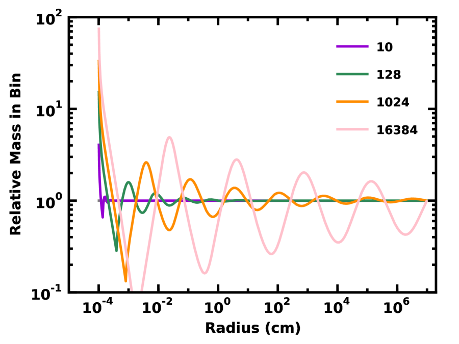
Figure 1: Relative mass distributions for equilibrium models of collisional cascades. The legend indicates $v^{2}/Q_{D}^{\star}$ for each curve. Systems with larger $v^{2}/Q_{D}^{\star}$ have more wavy mass distributions.

Fig. 1 compares the relative mass distributions for equilibrium solutions with different values of $v^{2}/Q_{D}^{\star}$. In systems with the simple power law ($N(r)\propto r^{-3.5}$), the relative mass distribution follows a straight horizontal line. For equilibrium mass distributions, the lack of grains with $r\leq r_{min}$ prevents collisional disruption of particles with $r\approx$ 1–3 $r_{min}$ and produces an excess of these objects (Campo Bagatin et al., 1994; O’Brien & Greenberg, 2003; Wyatt et al., 2011; Kenyon & Bromley, 2016). Similarly, the excess of particles just larger than $r_{min}$ produces a deficit of particles with $r\approx$ 10 $r_{min}$. At small $v^{2}/Q_{D}^{\star}$, the waviness in the relative mass distribution is minimal and confined to particle sizes $r\lesssim$ 10–30 $r_{min}$. As the adopted $v^{2}/Q_{D}^{\star}$ grows, the relative mass distribution becomes wavier and wavier at larger and larger sizes.

Along with dramatic changes in waviness as a function of $v^{2}/Q_{D}^{\star}$, these size distributions have very different ratios of the cross-sectional area ($A_{d}$) to the total mass of the swarm ($M_{d}$). In a standard power-law size distribution, $N\propto r^{-3.5}$, with $r_{min}$ = 1 $\rm\,\mu{\rm m}$ and $r_{max}$ = 100 km, ${M_{d}}/A_{d}\approx$ $12.65(r_{max}/{\rm 1~{}km})^{1/2}$. In wavy size distributions with $v^{2}/Q_{D}^{\star}$ = 8, $A_{d}/{M_{d}}$ is identical to the power-law ratio. The derived ${M_{d}}/A_{d}$ slowly drops with increasing $v^{2}/Q_{D}^{\star}$, falling by a factor of roughly 3 (10) when $v^{2}/Q_{D}^{\star}$ = $10^{3}$ ($10^{5}-10^{6}$). For $v^{2}/Q_{D}^{\star}$ $\leq 10^{3}$, decline in ${M_{d}}/A_{d}$ is fairly independent of $r_{max}$. At larger $v^{2}/Q_{D}^{\star}$, the amount of waviness and ${M_{d}}/A_{d}$ are more sensitive to $r_{max}$.

With $L_{d}\propto A_{d}$, systems with the equilibrium size distribution and $v^{2}/Q_{D}^{\star}$$\geq$ 10 require less mass to produce the same infrared excess. This mass monotonically decreases with increasing $v^{2}/Q_{D}^{\star}$.

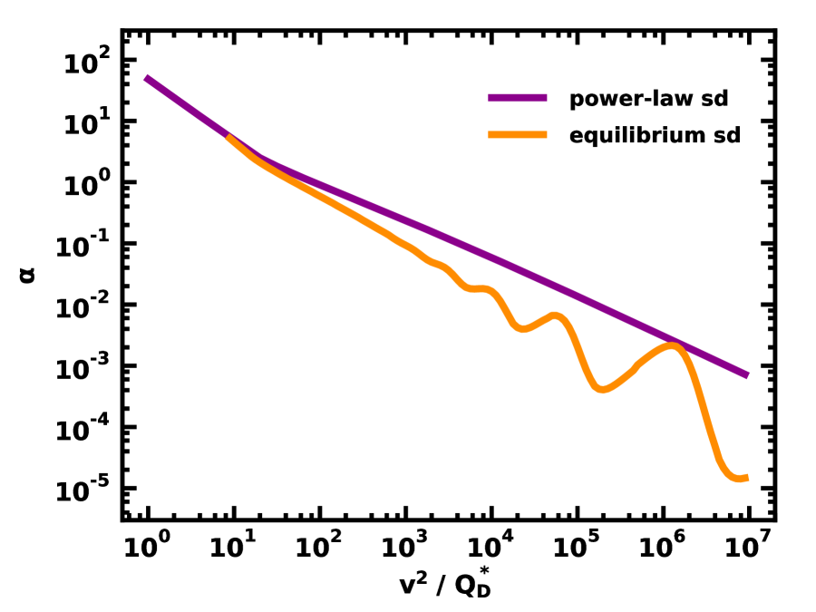
Figure 2: Collision time parameter $\alpha$ for power-law (magenta symbols) and equilibrium (orange symbols) size distributions. With $t_{c}=\alpha t_{0}$, systems with larger $v^{2}/Q_{D}^{\star}$ have shorter collision times. For equilibrium models, extremely wavy size distributions at large $v^{2}/Q_{D}^{\star}$ yield wavy behavior in $\alpha$.

Fig. 2 illustrates the impact of the adopted size distribution on $\alpha$ for a broad range of $v^{2}/Q_{D}^{\star}$. When $v^{2}/Q_{D}^{\star}\ \leq 8$, most collisions eject little mass from the combined object. With $\dot{M}_{d}$ small, $t_{c}$ is larger than $t_{0}$. As $v^{2}/Q_{D}^{\star}$ grows, collisions produce more and more debris. Systems with larger mass loss rates evolve more rapidly. Thus, $\alpha$ declines with $v^{2}/Q_{D}^{\star}$.

To construct a simple analytical relation for $\alpha$, we derive least-squares fits to the data in Fig. 2. Models with $\alpha=\alpha_{1}(v^{2}/Q_{D}^{\star})^{-e_{1}}+\alpha_{2}(v^{2}/Q_{D}^{\star})^{-e_{2}}$ yield $\alpha_{1}$ = 38.71, $e_{1}$ = 1.637, $\alpha_{2}$ = 16.32, and $e_{2}$ = 0.620 (power-law size distribution) and $\alpha_{1}$ = 13.00, $e_{1}$ = 1.237, $\alpha_{2}$ = 20.90, and $e_{2}$ = 0.793 (equilibrium size distribution). For the power-law size distribution, the model matches the data to better than 5% over the entire range in $v^{2}/Q_{D}^{\star}$. Although waviness in $\alpha$ for the equilibrium size distribution precludes such a good match for all $v^{2}/Q_{D}^{\star}$, the model agrees within 5% for $v^{2}/Q_{D}^{\star}\lesssim$ 3000.

To identify a second equation for $r_{max}$, we first set the boundary between catastrophic and cratering collisions. We define $f_{c}$ as the critical ratio of the collision energy $Q_{c}$ to the binding energy $Q_{D}^{\star}$ which separates catastrophic and cratering outcomes. If all particles have the same velocity $v$, collisions among more massive particles have larger center-of-mass collision energy $Q_{c}$. Thus, we can adopt a maximum $x$, $x_{cc}$, which results in a cratering collision. Collisions with $x>x_{cc}$ result in catastrophic outcomes.

In principle, establishing $x_{cc}$ is straightforward. Recalling the mass ejected in a collision when $b_{d}$ = 1, $m_{e}=0.5(m_{1}+m_{2})Q_{c}/Q_{D}^{\star}$, we require $Q_{c}/Q_{D}^{\star}<f_{c}$ for cratering and $Q_{c}/Q_{D}^{\star}\geq f_{c}$ for catastrophic fragmentation. Adopting a value for $f_{c}<$ 1 results in a quadratic equation for $x_{cc}^{3}$, which has real solutions for $v^{2}/Q_{D}^{\star}\geq 8f_{c}$ and one solution for $x_{cc}\ \leq$ 1.

With $x_{cc}$ known, we derive an expression for $\dot{r}_{max}=\dot{m}_{max}/4\pi\rho r_{max}^{2}$ = $-\int^{x_{cc}}_{0}~{}dx~{}dN_{1}/dt~{}(m_{e}~{}-~{}m_{2})$:

$$\dot{r}_{max}=-\left({\epsilon r_{0}\over 96t_{0}}\right)\left({v^{2}\over 4Q_{D}^{\star}}X_{1}(x_{cc})-X_{2}(x_{cc})\right)$$ (8)

where

$$X_{1}=\int^{x_{cc}}_{0}{x^{-1/2}(1+x)^{2}dx\over(1+x^{3})}=2~{}{\rm tan^{-1}}({x_{cc}^{1/2}\over x-1})~{}$$ (9)

and

$$X_{2}=\int^{x_{cc}}_{0}x^{-1/2}(1+x)^{2}dx=(3x_{cc}^{1/2}+10x_{cc}\ +15)\left({2x_{cc}^{1/2}\over 15}\right)~{}$$ (10)

Defining

$$\beta={\epsilon\alpha\over 96}\left({v^{2}\over 2Q_{D}^{\star}}X_{1}(x_{cc})-X_{2}(x_{cc})\right)~{},$$ (11)

we have a simple expression for $\dot{r}_{max}$:

$$\dot{r}_{max}=-\beta{M\over M_{0}}{r_{0}\over\alpha t_{0}}~{},$$ (12)

For the standard power-law size distribution $N(r)=N_{0}r_{max}^{-3.5}x^{-3.5}$, there is a simple solution to the system of two equations (eqs. 2 and 12) for the two unknowns $M$ and $r_{max}$:

$$r_{max}(t) = {r_{0}\over(1+t/\tau_{0})^{\gamma}}$$ (13)

$$M_{d}(t) = {M_{0}\over(1+t/\tau_{0})^{(1+\gamma)}}$$ (14)

where

$$\gamma=\frac{\beta}{1-\beta}$$ (15)

and

$$\tau_{0}=(\gamma+1)t_{c}=(\gamma+1)\alpha t_{0}~{}.$$ (16)

Using a more general expression for the size distribution – e.g., $N(r)\propto N_{0}f(x)r_{max}^{-3.5}x^{-3.5}$ where $f(x)$ is some function which relates the standard power-law to the general size distribution – leads to the same result except for modest changes to the integrals $X_{1}$ and $X_{2}$. Because our main focus is on the time variation of $r_{max}$ and $M_{d}$, we proceed with the solution in eqs. 13–16.

The form of the equations for $r_{max}$ and $M_{d}$ mirror those in the standard analytical model. When $r_{max}$ is constant in time, $\gamma$ = 0. At late times, $r_{max}$ and $M_{d}$ follow simple power laws: $r_{max}(t)=r_{0}(t/\tau_{0})^{-\gamma}$ and ${M_{d}}(t)=M_{0}(t/\tau_{0})^{-(\gamma+1)}$.

Connecting the evolution of $r_{max}$ and $M_{d}$ to the dust luminosity $L_{d}$ is straightforward. In the standard analytical model, $L_{d}=L_{0}/(1+t/t_{0})$, where $L_{0}$ depends on the total cross-sectional area $A_{d}$ of the swarm of solids. Expressing $A_{d}$ in terms of a time-dependent $M_{d}$ and $r_{max}$,

$$L_{d}={L_{0}\over(1+t/\tau_{0})^{-(1+\gamma/2)}}~{}.$$ (17)

In this expression, the $\gamma/2$ component results from the relationship between $L_{0}$ and $r_{max}$: $L_{0}\propto r_{max}^{-1/2}$.

Independent of the input parameters, the simple solutions for $r_{max}(t)$, $M_{d}(t)$, and $L_{d}(t)$ yield several robust results. At early times, the evolution follows standard analytical models with constant $r_{max}$: $M_{d}$ and $L_{d}$ fall to half of their initial values in one collision time $\alpha t_{0}$. After several collision times, $r_{max}$ starts to approach the asymptotic result, $r_{max}\ \propto t^{-\gamma}$. On the same time scale, $M_{d}$ and $L_{d}$ also begin to follow power-law declines with an exponent $1+\gamma$ for $M_{d}(t)$ and $1+\gamma/2$ for $L_{d}(t)$.

For any adopted $f_{c}\leq 1$, any initial size distribution, and any $v^{2}/Q_{D}^{\star}$ $\leq$ 4 ($v^{2}/Q_{D}^{\star}$ $\geq$ 5), the model predicts the largest objects grow (diminish) with time. Once $f_{c}$ is known, other aspects of the model (including a specific $v^{2}/Q_{D}^{\star}$ where $\dot{r}_{max}$ = 0) follow uniquely. In practice, however, there is no clear boundary between cratering and catastrophic collisions. For this study, we use the results of numerical simulations to establish $\tau_{0}$ and $\gamma$.

In addition to $f_{c}$, the analytic model relies on a constant $Q_{D}^{\star}$ and the exponents, $b_{d}$ and $b_{l}$, in the relations for the ejected mass and size of the largest object in the ejecta. Variations in $b_{l}$ have modest impact on the evolution of $r_{max}$, $M_{d}$, and $L_{d}$; however, small differences in $b_{d}$ produce measurable changes in the evolution of $r_{max}$ and $L_{d}$ (Kenyon & Bromley, 2016). While Kenyon & Bromley (2016) did not discuss how outcomes with constant $Q_{D}^{\star}$ differ from those where $Q_{D}^{\star}$ varies with $r$, they note that the evolution of $L_{d}$ in planet formation simulations is not sensitive to the form of $Q_{D}^{\star}$ (see also Kenyon & Bromley, 2008, 2010, 2012). We return to this issue in §3.3.

3 COMPARISON WITH NUMERICAL SIMULATIONS

To test the analytical model, we compare with results from numerical simulations of collisional cascades at 1 AU and at 25 AU. As in Kenyon & Bromley (2016), we use Orchestra, an ensemble of computer codes developed to track the formation and evolution of planetary systems. Within the coagulation component of Orchestra, we seed a single annulus with a swarm of solids having minimum radius $r_{min}$ and maximum radius $r_{max}$. The annulus covers 0.9–1.1 AU at 1 AU (22.5–27.5 AU at 25 AU). At 1 AU (25 AU), the solids have initial mass $M_{d}$ = 5 $\rm M_{\oplus}$ (700 $\rm M_{\oplus}$), mass density $\rho_{s}$ = 3 $\rm g~{}cm^{-3}$ (1.5 $\rm g~{}cm^{-3}$), surface density $\Sigma_{0}$ = 106 $\rm g~{}cm^{-2}$ (24 $\rm g~{}cm^{-2}$), and collision time $t_{0}\simeq 7.51\times 10^{3}$ yr ($2.07\times 10^{6}$ yr).

To evolve this system in time, the code derives collision rates and outcomes following standard particle-in-a-box algorithms. For these simulations, the initial size distribution of solids follows a power-law, $N\propto r^{-3.5}$, with a mass spacing between mass bins $\delta\equiv m_{i+1}/m_{i}$ = 1.05–1.10. The orbital eccentricity $e$ and inclination $i$ of all solids are held fixed throughout the evolution: $e_{0}$ = 0.1 at 1 AU (0.2 at 25 AU) and $i_{0}$ = $e_{0}/2$.

In any time step, all changes in particle number for $N\leq 2\times 10^{9}$ are integers. The collision algorithm uses a random number generator to round fractional collision rates up or down. This approach creates a realistic ‘shot noise’ in the collision rates which leads to noticeable fluctuations in $r_{max}$ and $L_{d}$ as a function of time.

Collision outcomes depend on the ratio $v^{2}/Q_{D}^{\star}$. In our approach, $v^{2}$ depends on $a$, $e$, $i$, and the mutual escape velocity of colliding particles. Although our formalism also includes gravitational focusing (Kenyon & Bromley, 2012, and references therein), focusing factors are of order unity. For simplicity, we set $Q_{D}^{\star}$ = constant; varying the constant allows us to evaluate how the evolution depends on the initial $v^{2}/Q_{D}^{\star}$. As $r_{max}$ declines with time, $v^{2}/Q_{D}^{\star}$ also slowly declines. Thus, we expect some deviations from the predictions of the analytical model. For additional details on algorithms in the coagulation code, see Kenyon & Luu (1998, 1999, and references therein); Kenyon & Bromley (2001, 2002a, and references therein); Kenyon (2002, and references therein); Kenyon & Bromley (2004, 2008, 2012, 2016, and references therein).

3.1 Results at 1 AU

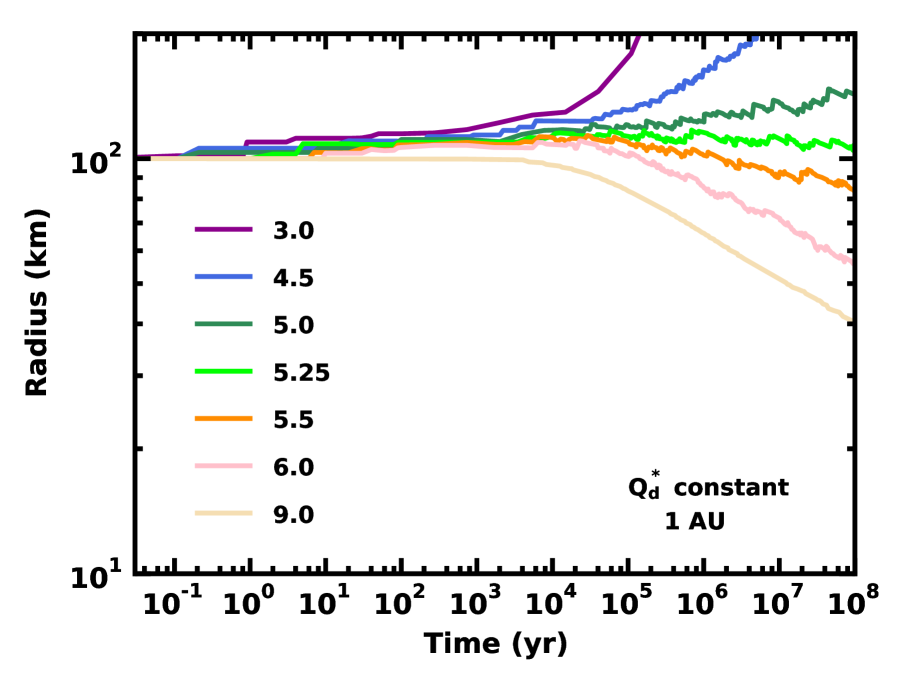
Figure 3: Time evolution of $r_{max}$, the size of the largest object in the cascade, as a function of $v_{2}/Q_{D}^{\star}$ for numerical simulations of collisional evolution at 1 AU. The legend associates $v^{2}/Q_{D}^{\star}$ with each curve. In systems with $v^{2}/Q_{D}^{\star}\lesssim$ 5.25, the largest object grows with time. When $v^{2}/Q_{D}^{\star}\gtrsim$ 5.25, catastrophic and cratering collisions steadily remove material from the largest objects.

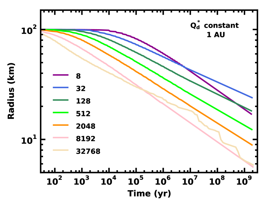
Figure 4: As in Fig. 3 for calculations with $v^{2}/Q_{D}^{\star}\geq$ 8. Systems with larger $v^{2}/Q_{D}^{\star}$ have more destructive collisions and generally evolve more rapidly.

Figs. 3–4 illustrate the evolution of the largest objects in a collisional cascade at 1 AU (see also Kenyon & Bromley, 2016). When $v^{2}/Q_{D}^{\star}\lesssim$ 8 (Fig. 3), collisions among equal-mass particles yield one larger merged object and a substantial amount of debris. Collisions with smaller particles always produce debris and may augment the mass of the larger object.

The balance between accretion and mass loss depends on $v^{2}/Q_{D}^{\star}$. For this suite of simulations where $Q_{D}^{\star}$ is independent of particle mass density and radius, the largest objects gain (lose) mass when $v^{2}/Q_{D}^{\star}\leq$ 5.0 ($v^{2}/Q_{D}^{\star}\geq$ 5.5). When $v^{2}/Q_{D}^{\star}\ \approx$ 5.0–5.5, growth and destruction roughly balance. Depending on the mix of collisions as the system evolves, $r_{max}$ sporadically increases and decreases. This critical value for $v^{2}/Q_{D}^{\star}$ is close to the value of 4–5 predicted from the analytical model.

In systems with much larger $v^{2}/Q_{D}^{\star}$ (Fig. 4), the collision time generally decreases monotonically with increasing $v^{2}/Q_{D}^{\star}$. As predicted by the analytical model, systems with larger $v^{2}/Q_{D}^{\star}$ initially evolve more rapidly. Once $r_{max}$ begins to decline, however, three evolutionary trends emerge. When $v^{2}/Q_{D}^{\star}$ $\approx$ 8–12, $r_{max}$ declines rather rapidly. When $v^{2}/Q_{D}^{\star}$ $\geq 10^{4}$ , the initially rapid evolution in $r_{max}$ slows considerably and then fluctuates dramatically. At intermediate values (12 $\leq v^{2}/Q_{D}^{\star}\leq 10^{4}$), $r_{max}$ evolves much more smoothly at an intermediate rate.

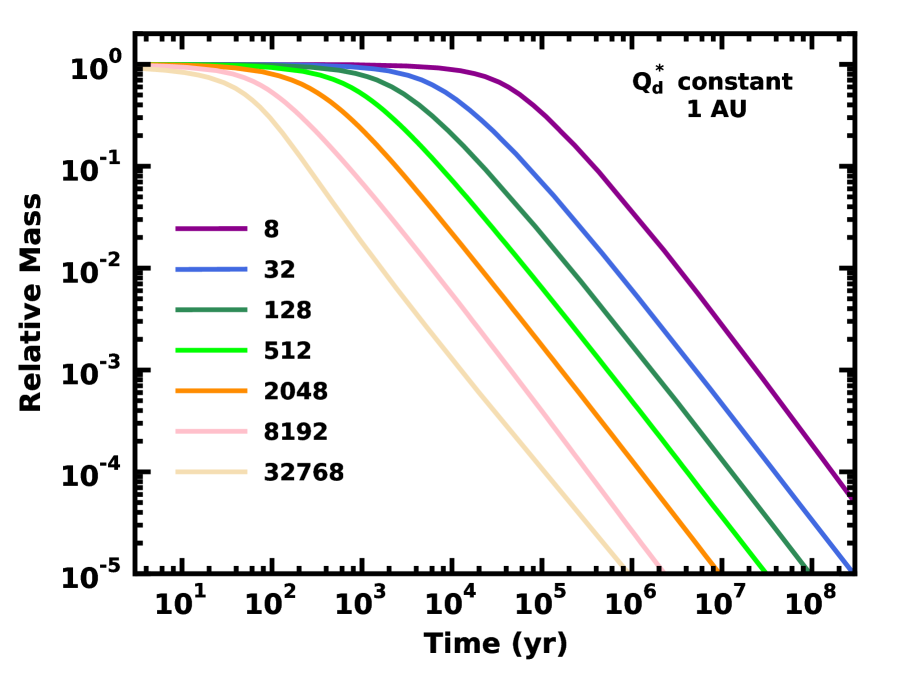
Figure 6: As in Fig. 4 for the total mass.

These differences have simple physical explanations. When $v^{2}/Q_{D}^{\star}$ $\gtrsim 10^{4}$, the collision parameter $\alpha\lesssim 10^{-2}$ (Fig. 2). With a short collision time, $t_{c}=\alpha t_{0}\lesssim 10^{3}$ yr, the system loses mass rapidly (see Fig. 6 below). Within 1 Myr, the system loses 99.99% of its initial mass. At this point, collisions among the largest objects are sporadic; shot noise dominates the evolution.

When $v^{2}/Q_{D}^{\star}\ \approx$ 8–12, only collisions among roughly equal mass objects yield catastrophic outcomes. Collisions between one object and a much smaller particle yield some growth and some debris. After several collisions times, systems with $v^{2}/Q_{D}^{\star}\approx$ 8–12 have (i) relatively more mass in the largest objects and (ii) shorter collision times than those systems with $v^{2}/Q_{D}^{\star}\gtrsim$ 12. As a result, the largest objects evolve somewhat faster at later times when $v^{2}/Q_{D}^{\star}\approx$ 8.

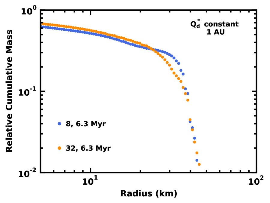
Figure 5: Relative cumulative mass distributions at 6 Myr for calculations with $r_{max}$ = 45 km and either $v^{2}/Q_{D}^{\star}$ = 8 (blue points) or $v^{2}/Q_{D}^{\star}$ = 32 (orange points). Despite identical $r_{max}$, the calculation with smaller $v^{2}/Q_{D}^{\star}$ has more total mass and more (less) mass in objects with $r\gtrsim$ 25 km ($\lesssim$ 25 km). The system with $v^{2}/Q_{D}^{\star}$ = 8 thus evolves more rapidly than the system with $v^{2}/Q_{D}^{\star}$ = 32.

To illustrate this point, Fig. 5 compares mass distributions for calculations with $v^{2}/Q_{D}^{\star}$ = 8 and 32 at 6 Myr, when both have the same $r_{max}$. The plot shows the relative cumulative mass distribution, defined as the cumulative mass from $r_{max}$ to $r$, $M_{d}(>r)$, relative to the total mass $M_{d}$ in the grid. This ratio grows from roughly $10^{-2}$ at $r=r_{max}$ to unity at $r=r_{min}$. For these two calculations, it is clear that the system with $v^{2}/Q_{D}^{\star}$ = 8 has relatively more mass in solids with $r\gtrsim$ 25 km and somewhat less mass in solids with $r\lesssim$ 25 km.

In addition to having more mass in large objects, the calculation with $v^{2}/Q_{D}^{\star}$ = 8 also has more mass overall. Systems with more mass have shorter collision times (eq. 1). At late times, systems with $v^{2}/Q_{D}^{\star}$ $\approx$ 8–10 evolve more rapidly than systems with $v^{2}/Q_{D}^{\star}$ $\approx$ 16–32.

For intermediate $v^{2}/Q_{D}^{\star}$, the evolution more closely follows expectations from the analytical model. Most collisions remove mass from the largest objects throughout the evolution. Thus, these objects gradually diminish in size as the total mass in the system declines.

Despite differences in the evolution of $r_{max}$, all systems with a declining $r_{max}$ lose mass on roughly the collision time scale $\tau_{0}=\alpha(\gamma+1)t_{0}$ (Fig. 6). Although there is some shot noise at large $v^{2}/Q_{D}^{\star}$ and some growth at small $v^{2}/Q_{D}^{\star}$, the total disk mass always drops smoothly with time. Systems with larger $v^{2}/Q_{D}^{\star}$ lose mass more rapidly.

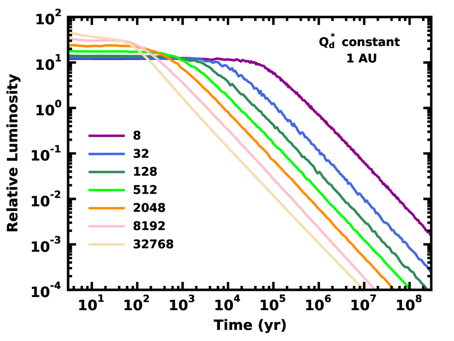
Figure 7: As in Fig. 4 for the total luminosity.

The dust luminosity generally follows the evolution of the total mass (Fig. 7). In every calculation, it takes 10–100 yr for the size distribution to reach an approximate equilibrium where the flow of mass from the largest particles to the smallest particles is similar throughout the grid. Systems with larger $v^{2}/Q_{D}^{\star}$ tend to reach this equilibrium more rapidly and at a somewhat larger $L_{d}$ than systems with smaller $v^{2}/Q_{D}^{\star}$. Once this period ends, the luminosity follows a power-law decline with superimposed spikes in $L_{d}$ due to shot noise.

These results demonstrate that the numerical simulations generally evolve along the path predicted by the analytical model. After a brief period of constant $r_{max}$, $M_{d}$, or $L_{d}$, these physical variables follow a power-law decline in time. To infer the slope of the power-law for each calculation, we perform a least-squares fit to $r_{max}(t)$, ${M_{d}}(t)$, and ${L_{d}}(t)$. Using an amoeba algorithm (Press et al., 1992), we derive the parameters $\tau_{0}$ and $\gamma$ from results for $r_{max}(t)$ and ${M_{d}}(t)$. Because our calculations relax to an equilibrium size distribution, we add a third parameter $L_{0}$ to fits for ${L_{d}}(t)$. Once the fitting algorithm derives these parameters, it is straightforward to infer $\alpha$ and $\beta$ using eq. 1, eq. 15, and eq. 16.

For the complete ensemble of calculations, the amoeba finds each solution in 20–25 iterations. Typical errors in the fitting parameters for $r_{max}$ and $M_{d}$ are $\pm$10%–20% in $\tau_{0}$ and $\pm$ 0.005 in $\gamma$. Among calculations with identical starting conditions, typical variations in the fitting parameters are $\pm$5%–10% in $\tau_{0}$ and $\pm 0.003$ in $\gamma$. Thus, intrinsic fluctuations in $\alpha$ and $\gamma$ are comparable to the fitting uncertainties. Adding the uncertainties in quadrature, the errors are $\pm$11%–22% in $\alpha$ and $\pm 0.006$ in $\gamma$.

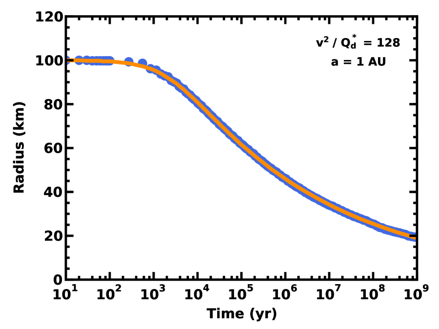
Figure 8: Evolution of $r_{max}$ in numerical simulations (filled blue circles) and in the new analytical model (solid orange curve) for a system with $Q_{D}^{\star}=2\times 10^{8}$ erg g^-1 at 1 AU. The analytical model matches the numerical calculation to better than 1% over $10^{1}$–$10^{9}$ yr.

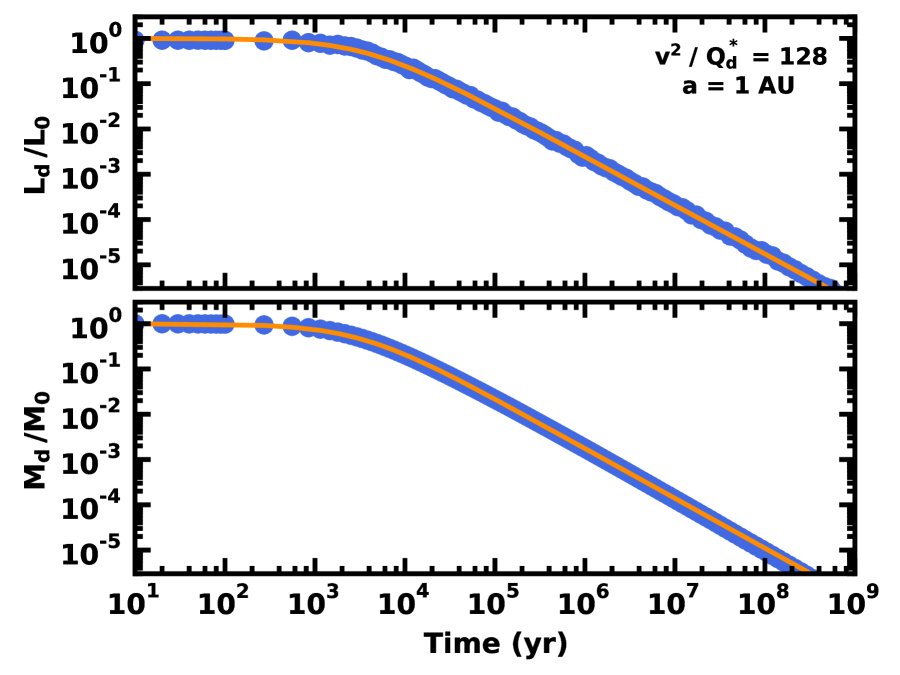
Figure 9: As in Fig. 8 for the relative disk mass (lower panel) and the relative disk luminosity (upper panel). The analytical model matches the numerical calculation to better than 0.5% in $M_{d}/M_{0}$ and better than 1.5% in $L_{d}/L_{0}$.

Figs. 8–9 show fits to one set of results for $v^{2}/Q_{D}^{\star}$ = 128. The model $r_{max}(t)=r_{0}/(1+t/\tau_{0})$ fits the data in Fig. 8 well: the agreement is excellent for $t\leq 10^{4}$ yr and $t\geq 10^{5}$ yr. In between these times, there is a small amount of ‘ringing’ as the numerical calculation settles down to the standard power-law evolution. For $L_{d}$ and $M_{d}$ (Fig. 9), the agreement between the numerical calculation and the model fits is also excellent.

In this example and all other calculations, the evolution of $M_{d}$ matches the model more closely than the evolution of $r_{max}$ or $L_{d}$. As these systems evolve, changes in $L_{d}$ and $r_{max}$ consist of a general decline due to the loss of mass and random fluctuations due to the shot noise inherent in our collision algorithm. Because larger input $v^{2}/Q_{D}^{\star}$ yields shorter collision times, these fluctuations grow with increasing $v^{2}/Q_{D}^{\star}$. Adopting an appropriate measure of these fluctuations enables fits with $\chi^{2}$ per degree of freedom of roughly unity.

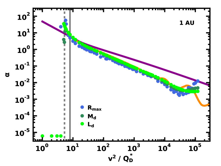
Figure 10: Variation of the derived collision time scale coefficient $\alpha$ as a function of $v^{2}/Q_{D}^{\star}$ for collisional cascade calculations at 1 AU. Vertical grey lines mark $v^{2}/Q_{D}^{\star}$ = 5.25 (dashed) and 8 (solid). Other solid curves repeat results from the analytical model in Fig. 2 for the power-law (magenta) and equilibrium (orange) size distribution. The numerical results closely follow the analytical model with the equilibrium size distribution. The legend associates symbol color with results for $r_{max}$, $M_{d}$, and $L_{d}$

For the complete ensemble of calculations, the derived $\alpha$ from fits to the evolution of $r_{max}$, $M_{d}$, and $L_{d}$ closely follows predictions for the analytical model using the equilibrium size distribution (Fig. 10). Remarkably, independent fits to the evolution of $M_{d}$ and $L_{d}$ for the same calculation yield nearly identical results for $\alpha$. For the evolution of $r_{max}$, derived values for $\alpha$ are typically 5% to 10% smaller. Although this offset is systematic, it is small compared to the uncertainties in model parameters derived from the amoeba fits. As expected, the analytical model provides a poor description of the numerical simulations when $v^{2}/Q_{D}^{\star}$ $\lesssim$ 8 and growth by mergers is an important process in the overall evolution of the swarm. When $10\lesssim v^{2}/Q_{D}^{\star}\lesssim 10^{4}$, however, the numerical results for $\alpha$ follow the predicted slope very well.

Once $v^{2}/Q_{D}^{\star}\gtrsim 10^{4}$, the analytical model predicts the numerical results rather poorly. For these large collision velocities, the evolution of $r_{max}$, $M_{d}$, and $L_{d}$ diverge dramatically from each other and from the analytic prediction. We associate this divergence with intrinsic shot noise (which grows as $M_{d}$ drops) and the appearance of extreme waviness in the size distribution (which causes large fluctuations in the evolution of $r_{max}$, $M_{d}$, and $L_{d}$).

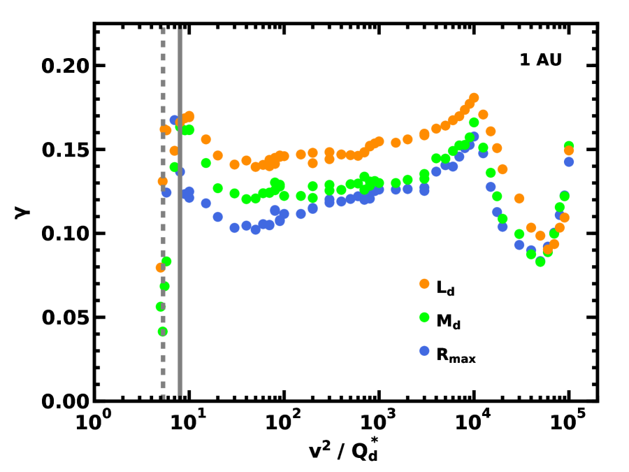
Figure 11: As in Fig. 10 for the power-law slope $\gamma$ for the evolution of $r_{max}$. Although the numerical results yield similar values of $\gamma$ for the evolution of $r_{max}$ and $M_{d}$, the luminosity $L_{d}$ has a larger $\gamma$ and evolves somewhat more rapidly than expected.

Derived values for $\gamma$ also show clear trends with $v^{2}/Q_{D}^{\star}$ (Fig. 11). As $v^{2}/Q_{D}^{\star}$ grows, $\gamma$ declines from 0.15 to 0.1, rises slowly to 0.15, and then fluctuates dramatically. There is a modest offset in $\gamma$ for $r_{max}$, $M_{d}$, and $L_{d}$. When $10\lesssim v^{2}/Q_{D}^{\star}\ \lesssim 10^{4}$, $\gamma({L_{d}})\approx\gamma({M_{d}})+0.02\approx\gamma(r_{max})+0.01$. Once $v^{2}/Q_{D}^{\star}\gtrsim 10^{4}$, $\gamma({M_{d}})\approx\gamma(r_{max})$; $\gamma({L_{d}})\approx\gamma(r_{max})+0.01$. These systematic offsets are 2–3 times larger than the uncertainties in $\gamma$ derived from the amoeba algorithm.

Although the numerical value for $\gamma$ depends on many details, the overall trends agree with predictions of the analytical model. As $v^{2}/Q_{D}^{\star}$ grows, collisions are more destructive; the largest objects are diminished more rapidly, which results in a larger value for $\gamma$. Once $v^{2}/Q_{D}^{\star}\gtrsim 10^{4}$, the extreme waviness in the size distribution sets the evolution of $r_{max}$; the analytical model then provides a poor description of the system.

For this suite of calculations, the typical $\gamma\approx$ 0.10–0.15 implies $\beta\approx$ 0.09–0.13. Recalling our definition in eq. 11, the slow variation of $\beta$ as a function of $v^{2}/Q_{D}^{\star}$ implies changes in $f_{c}$ with $v^{2}/Q_{D}^{\star}$. We infer $f_{c}\approx$ 1 for $v^{2}/Q_{D}^{\star}$ $\approx$ 10, $f_{c}\approx$ 0.04 for $v^{2}/Q_{D}^{\star}$ $\approx$ 100, $f_{c}\approx 10^{-3}$ for $v^{2}/Q_{D}^{\star}$ $\approx 10^{3}$, and $f_{c}\approx 3\times 10^{-5}$ for $v^{2}/Q_{D}^{\star}$ $\approx 10^{4}$. The progressive decline in $f_{c}$ with increasing $v^{2}/Q_{D}^{\star}$ implies a gradual reduction in the importance of cratering collisions as the collision energy grows. This result is sensible: larger collision energies result in greater frequency of catastrophic collisions.

3.2 Results at 25 AU

Predictions for the analytical model in §2 are independent of $a$. However, performing a suite of calculations at a different $a$ serves several goals: (i) we make a more robust connection between new calculations and those of previous investigators at $a$ = 10–50 AU (e.g., Krivov et al., 2005, 2006; Löhne et al., 2008; Gáspár et al., 2012a, b), (ii) we develop a better understanding of the impact of the mass resolution, stochastic variations, and timestep choices within our code, and (iii) we infer the impact of changing the particle density $\rho$. The analytical model is independent of $\rho$ (§2); however, the numerical model uses $\rho$ to calculate the escape velocity of colliding particles, which appears in expressions for the gravitational focusing factor and the impact velocity. Although we expect a minor impact on the evolution, changing $\rho$ might modify $f_{c}$ and the mix of cratering and catastrophic collisions.

Aside from a longer collision time, results at 25 AU closely follow those at 1 AU. In systems with $v^{2}/Q_{D}^{\star}\leq$ 5.0 ($v^{2}/Q_{D}^{\star}\geq$ 5.5), large objects gradually gain (lose) mass with time. For intermediate $v^{2}/Q_{D}^{\star}\approx$ 5.0–5.5, the evolution of the largest objects is more chaotic, with mass gain in some periods and mass loss during other epochs. After 10–20 Gyr of evolution with $v^{2}/Q_{D}^{\star}\approx$ 5.0–5.5, $r_{max}$ is roughly equal to $r_{0}$. Compared to calculations at 1 AU, the difference in $\rho$ has little influence on the critical $v^{2}/Q_{D}^{\star}$ required to balance growth and destruction.

For $10\lesssim v^{2}/Q_{D}^{\star}\lesssim 10^{4}$, the evolution of $r_{max}$, $M_{d}$, and $L_{d}$ follow the analytic model. Calculations with $v^{2}/Q_{D}^{\star}\approx$ 8–10, evolve somewhat more rapidly than those with $v^{2}/Q_{D}^{\star}\ \approx$ 20–30, but more slowly than those with $v^{2}/Q_{D}^{\star}\ \gtrsim$ 100–200. Once $v^{2}/Q_{D}^{\star}\gtrsim 10^{4}$, collision rapidly exhaust the mass reservoir, leaving the system with few large particles. Shot noise then dominates the decline of $r_{max}$.

The analytical model generally fits the evolution of $r_{max}$, $M_{d}$, and $L_{d}$ extremely well. For $v^{2}/Q_{D}^{\star}\approx$ 5–$10^{4}$, the amoeba fits derive robust results for the fitting parameters $\alpha$, $\gamma$, and $L_{0}$. In calculations with $v^{2}/Q_{D}^{\star}\lesssim$ 5, the largest objects grow with time; shot noise in the growth (debris production) rate often leads to poorer fits to the time evolution of $r_{max}$ ($L_{d}$). Because $M_{d}$ declines in all calculations, the analytical model fits the time evolution of $M_{d}$ even when $v^{2}/Q_{D}^{\star}$ is small. However, the evolution of $M_{d}$ when $v^{2}/Q_{D}^{\star}\lesssim$ 5 is much slower than the evolution of systems with larger $v^{2}/Q_{D}^{\star}$.

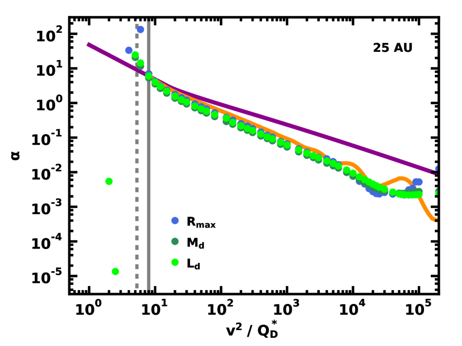
Figure 12: As in Fig. 10 for calculations at 25 AU.

Despite substantial differences in the initial mass and a modest change in $\rho$, calculations at 25 AU yield nearly the same variation of $\alpha$ with $v^{2}/Q_{D}^{\star}$ as those at 1 AU (Fig. 12). For $v^{2}/Q_{D}^{\star}\gtrsim$ 8–10, results closely follow predictions of the analytical model for the equilibrium size distribution. Results for the fits to $r_{max}$ are somewhat closer to these predictions than results for fits to $M_{d}$ and $L_{d}$. However, the differences are fairly negligible compared to the uncertainties in amoeba model fits for $\alpha$.

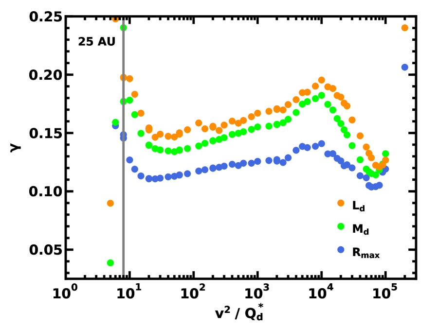
Figure 13: As in Fig. 11 for calculations at 25 AU.

As in the calculations at 1 AU, $\gamma$ clearly correlates with $v^{2}/Q_{D}^{\star}$ (Fig. 13). Although the overall trends in $\gamma$ with $v^{2}/Q_{D}^{\star}$ are similar at 1 AU and 25 AU, results at 25 AU show a somewhat larger displacement between the different models. At 25 AU, $\gamma({M_{d}})\approx\gamma(r_{max})+g_{1}$ with $g_{1}\approx$ 0.03–0.05 instead of 0.01–0.03. Similarly $\gamma({L_{d}})\approx\gamma(r_{max})+g_{2}$ with $g_{2}\approx$ 0.04–0.07 instead of 0.03–0.04.

Calculations at 25 AU also result in somewhat different variations in $f_{c}$ with $v^{2}/Q_{D}^{\star}$. For $v^{2}/Q_{D}^{\star}$ = 10–300, $f_{c}$ derived at 25 AU tracks results at 1 AU very closely. When $v^{2}/Q_{D}^{\star}$ = 300–$10^{4}$, $f_{c}$ is smaller: $5\times 10^{-4}$ at $v^{2}/Q_{D}^{\star}$ = 1000 (instead of $10^{-3}$) and $2\times 10^{-5}$ at $v^{2}/Q_{D}^{\star}$ = 10000 (instead of $3\times 10^{-5}$). Compared to the overall change in $f_{c}$ with $v^{2}/Q_{D}^{\star}$, these differences are relatively minor.

3.3 Discussion

The comparisons between results of the numerical simulations and expectations from the analytical model are encouraging. Within the full set of several hundred simulations at 1 AU and at 25 AU, the derived evolution of $r_{max}$, $M_{d}$, and $L_{d}$ matches the predictions almost exactly. Repeat calculations with identical starting conditions yield nearly identical values for $\alpha$ and $\gamma$. Changing the particle mass density $\rho$ has minor impact on the results. We conclude that the analytical model provides an accurate representation of numerical simulations for collisional cascades with a fixed $v^{2}/Q_{D}^{\star}$. In the rest of this section, we consider comparisons of our results with previous studies and discuss how $\gamma$ depends on various aspects of the calculations.

Previous estimates for the collision time parameter $\alpha$ yield a broad range of results. Analytical estimates for $v^{2}/Q_{D}^{\star}$ $\gg$ 1 suggest $\alpha\propto(v^{2}/Q_{D}^{\star})^{-p}$ with $p$ = 5/6 (e.g., Löhne et al., 2008; Kobayashi & Tanaka, 2010; Wyatt et al., 2011, and references therein). Although some numerical calculations confirm the analytical result (Kobayashi & Tanaka, 2010), others suggest $p$ = 1.125 (Löhne et al., 2008) or $p$ = 1 (Kenyon & Bromley, 2016).

Our analysis clarifies these disparate results. For a broad range of $v^{2}/Q_{D}^{\star}$, we infer $\alpha=\alpha_{1}(v^{2}/Q_{D}^{\star})^{-e_{1}}+\alpha_{2}(v^{2}/Q_{D}^{\star})^{-e_{2}}$ with $\alpha_{1}$ = 38.71, $e_{1}$ = 1.637, $\alpha_{2}$ = 16.32, and $e_{2}$ = 0.620 for a power-law size distribution and $\alpha_{1}$ = 13.00, $e_{1}$ = 1.237, $\alpha_{2}$ = 20.90, and $e_{2}$ = 0.793 for the equilibrium size distribution. All previous analytical studies of $\alpha$ for $v^{2}/Q_{D}^{\star}\gg$ 1 (Löhne et al., 2008; Kobayashi & Tanaka, 2010; Wyatt et al., 2011) agree reasonably well with our expectation for the equilibrium size distribution. In numerical simulations, the derived size distribution generally follows the equilibrium size distribution (Kenyon & Bromley, 2016). For the range of $v^{2}/Q_{D}^{\star}$ investigated in Löhne et al. (2008) and Kenyon & Bromley (2016) – $v^{2}/Q_{D}^{\star}$ $\lesssim$ 200 – the predicted slope for a single power-law fit to $\alpha$ is 1–1.1, as inferred in these two studies. When $v^{2}/Q_{D}^{\star}$ is much larger (as in Kobayashi & Tanaka, 2010), the expected slope is close to 0.8. Thus, various numerical calculations of collisional cascades are consistent with one another.

Despite the good general agreement between the analytical model and the numerical calculations, there is one clear difference. At late times, the analytical model predicts $M_{d}L_{d}^{-1}r_{max}^{-1/2}\propto t^{-g}$, with $g\equiv$ 0. In the numerical calculations, $g\neq$ 0. The non-zero $g$ produces offsets in plots of $\gamma(r_{max})$, $\gamma({M_{d}})$, and $\gamma({L_{d}})$ as functions of $v^{2}/Q_{D}^{\star}$ (Figs. 11 and 13).

Fig. 14 shows the variation of $g$ with $v^{2}/Q_{D}^{\star}$. Overall, the deviation from the prediction is rather small. Although the displacements from zero are somewhat different, the trends at 1 AU (blue circles) and at 25 AU (orange circles) are similar: (i) a decreasing $g$ at $v^{2}/Q_{D}^{\star}$ = 10–100, (ii) a roughly constant $g$ at $v^{2}/Q_{D}^{\star}$ = 100–$10^{4}$, and (iii) an oscillation at $v^{2}/Q_{D}^{\star}$$\gtrsim 10^{4}$. Results at 25 AU are somewhat closer to the analytical prediction than results at 1 AU.

The offset of $g$ from zero results from an inability of the numerical simulations to maintain an equilibrium size distribution. Throughout every calculation, the derived size distribution is similar but not identical to the analytical equilibrium size distribution described in §2. As calculations proceed, the numerical size distribution also wanders farther away from equilibrium. Relative to an equilibrium size distribution with $r_{min}$ = 1 $\rm\,\mu{\rm m}$ and arbitrary $r_{max}$, the numerical size distribution usually has somewhat less total mass and always has less cross-sectional area. Thus, $M_{d}$ and $L_{d}$ decline faster than $r_{max}$ relative to the predictions of the analytical model.

There are several possible origins for ‘non-equilibrium’ size distributions in our calculations, (i) shot noise in the collision rate of the largest objects, (ii) non-zero $r_{min}$ and finite $r_{max}$, and (iii) finite mass resolution $\delta$ and timestep $\delta t$. The tests outlined below indicate that differences in $\rho$ have little influence on the variation of $g$ with $v^{2}/Q_{D}^{\star}$.

Throughout the course of the evolution, the size distribution is the sum of two components: (i) an equilibrium piece produced by the steady collisional grinding of objects with $r\lesssim$ 0.1–0.3 $r_{max}$ and (ii) waves of debris generated by occasional collisions among pairs of the largest objects with $r\gtrsim$ 0.1–0.3 $r_{max}$. Test calculations demonstrate that steady collisional grinding, without pulses of debris from collisions of larger objects, yield size distributions close to the equilibrium size distribution with $g$ almost zero. During the pulses, however, the size distribution deviates considerably from equilibrium, changing the relationship between $M_{d}$, $A_{d}$ (and thus $L_{d}$), and $r_{max}$. Despite the large variations in the size distribution, $g$ is still fairly close to zero.

In calculations at 25 AU, the larger initial mass reduces shot noise compared to the calculations at 1 AU. Several calculations with a factor of ten more mass at either $a$ reduce the absolute value of $g$. Thus, shot noise is clearly responsible for some of the deviations of the numerical calculations from the predictions of the analytical model.

The non-zero $r_{min}$ and the finite $r_{max}$ also contribute significantly to the non-equilibrium size distribution. For example, when $r_{min}$ = 1 $\rm\,\mu{\rm m}$ ($10^{-3}$ $\rm\,\mu{\rm m}$), $r_{max}$ = 10–100 km, and $v^{2}/Q_{D}^{\star}$ $\approx$ 100, waviness in the equilibrium size distribution occurs for $r\lesssim$ 1–10 cm (10–100 $\rm\,\mu{\rm m}$; see Fig. 1). Pulses from collisions of 10–100 km objects yield an extra waviness at $r\lesssim$ 0.1–1 km. Several test calculations suggest that the ability of the numerical calculation to ‘smooth out’ this extra waviness depends on the size range between the two sets of waves in the size distribution: reducing $r_{min}$ allows collisional processes to reduce the amplitude of the pulse before it reaches the intrinsic waviness caused by the non-zero $r_{min}$. In these calculations, $g$ is closer to zero for $v^{2}/Q_{D}^{\star}$ $\lesssim$ 100.

This feature of the numerical calculations explains the trends in Fig. 14. For $v^{2}/Q_{D}^{\star}$ $\gtrsim$ 1000, the finite $r_{min}$ produces large waves in the equilibrium size distribution where shot noise generates pulses in debris production. The combination of an intrinsically wavy size distribution at 1–10 km and wave-like pulses of debris generated from infrequent collisions of 100 km objects yields a very non-equilibrium size distribution where the evolution of $M_{d}$ and $L_{d}$ are less correlated with the evolution of $r_{max}$. Thus, $g$ varies rapidly with $v^{2}/Q_{D}^{\star}$.

Test calculations suggest that adopting smaller $r_{min}$ and larger initial $r_{max}$ change the placement of the waves in the relation between $g$ and $v^{2}/Q_{D}^{\star}$ illustrated in Fig. 14. Reducing $r_{min}$ also tends to force $g$ closer to zero; the change is more dramatic for calculations with $v^{2}/Q_{D}^{\star}$ $\lesssim$ 100 than for those with $v^{2}/Q_{D}^{\star}$ $\gtrsim$ 1000. For these large values of $v^{2}/Q_{D}^{\star}$, it is necessary to increase the initial $r_{max}$ significantly to change $g$ dramatically.

Finally, the finite mass resolution and the need for finite time steps limit the ability of the coagulation calculations to track the analytical model. Figs. 25–26 of Kenyon & Bromley (2016) show how finer mass resolution reduces the noise in numerical calculations of wavy size distributions. Although simulations for this paper with $\delta$ = 1.05–1.10 match analytical predictions very well, calculations with smaller $\delta$ would improve the agreement. Taking smaller time steps cannot change the impact of a pulse of debris on the size distribution; however, smaller steps allow the code to smooth out the pulses more evenly. Calculations with smaller $\delta$ and $\delta t$ are very cpu-intensive. Given the small differences between the predictions of the analytical model and the results of the numerical simulations, more accurate calculations are not obviously worthwhile.

For models where $Q_{D}^{\star}$ is a function of radius, we expect similar results. Adopting an expression appropriate for rocky solids at 1 AU, $Q_{D}^{\star}$ = $3\times 10^{7}r^{-0.4}$ + $0.3\rho r^{1.35}$ (e.g., Kenyon & Bromley, 2016), $v^{2}/Q_{D}^{\star}$ $\approx$ 50 for collisions between pairs of 100 km objects. Within a suite of 10 calculations using parameters otherwise identical to our calculations with constant $Q_{D}^{\star}$, the variations in $\gamma(r_{max})$, $\gamma({M_{d}})$, and $\gamma({L_{d}})$ are small, 0.01–0.02, as in calculations with constant $Q_{D}^{\star}$. Overall, the $\gamma(r_{max})$ values are 0.03–0.05 smaller when $Q_{D}^{\star}$ is a function of radius. The offsets between $\gamma({M_{d}})$, $\gamma({L_{d}})$ and $\gamma(r_{max})$ are similar, $\sim$ 0.02–0.04.

This difference has a simple physical origin. When $Q_{D}^{\star}$ is a function of radius, $v^{2}/Q_{D}^{\star}$ is larger for all solids with $r\leq$ 10 km than for larger particles. With larger $v^{2}/Q_{D}^{\star}$, the mass in small particles declines more rapidly than the mass in large objects. Calculations with $Q_{D}^{\star}(r)$ then have less mass in small particles than those with constant $Q_{D}^{\star}$ (e.g., Fig. 15 of Kenyon & Bromley, 2016). Compared to a calculation with the same mass in large objects and constant $Q_{D}^{\star}$, large objects with $Q_{D}^{\star}(r)$ suffer fewer cratering collisions and therefore less mass loss; $r_{max}$ then declines more slowly with time. Although the overall $L_{d}$ is smaller, it also declines more slowly with time. Thus, the $\gamma$ factors are somewhat smaller.

Despite the sensitivity of our numerical results to various choices, applications of the analytical model to real data are probably rather insensitive to the choice of $\gamma$ among the various possibilities. We suggest setting $\gamma$ = $\gamma(r_{max})$ = 0.12 for $v^{2}/Q_{D}^{\star}$ $\lesssim$ 100–1000 and $\gamma$ = $\gamma(r_{max})$ = 0.13 for $v^{2}/Q_{D}^{\star}$ $\gtrsim$ 1000. In most real systems, the mass of the swarm is rarely large enough to prevent shot noise from impacting the evolution. The evolution of the cascade then probably deviates from the predictions of the analytical model. In these circumstances, adopting $\gamma({M_{d}})=\gamma(r_{max})+0.02$ and $\gamma({L_{d}})=\gamma(r_{max})+0.03$ should provide an adequate representation of the evolution of a real system.

Even though $\gamma$ is small, the evolution of $r_{max}$ still has an impact on the late time evolution of the dust luminosity. After 10–1000 collision times, systems with a changing $r_{max}$ are from 15% to 40% fainter than those with a static $r_{max}$. Producing a specific $L_{d}$ late in the evolution therefore requires a system with a larger initial mass relative to the standard analytical model. For some circumstances, the required initial mass is as much as a factor of two larger.

4 SUMMARY

We have developed a new analytical model for the evolution of a collisional cascade in a ring of solid particles orbiting a massive central object. In our derivation for systems with a constant $v^{2}/Q_{D}^{\star}$, $r_{max}$ the radius of the largest object in the cascade evolves as $r_{max}=r_{0}(1+t/t_{c})^{-\gamma}$, where $r_{0}$ is the initial radius of the largest object, $t_{c}=\alpha(\gamma+1)t_{0}$, $t_{0}=r_{0}\rho P/12\pi\Sigma_{0}$, and $\gamma$ is a constant which depends on $f_{c}$ the ratio of the collision energy to the critical collision energy required for catastrophic collisions. The mass $M_{d}$ and the luminosity $L_{d}$ of the solids then evolve as ${M_{d}}=M_{0}(1+t/t_{c})^{-(\gamma+1)}$ and ${L_{d}}=L_{0}(1+t/t_{c})^{-(\gamma/2+1)}$. The collision time scale parameter $\alpha$ is a simple function of $v^{2}/Q_{D}^{\star}$: $\alpha=\alpha_{1}(v^{2}/Q_{D}^{\star})^{-e_{1}}+\alpha_{2}(v^{2}/Q_{D}^{\star})^{-e_{2}}$ with $\alpha_{1}$ = 13.00, $e_{1}$ = 1.237, $\alpha_{2}$ = 20.90, and $e_{2}$ = 0.793.

The new model applies to cascades in a single annulus of width $\delta a\geq ae$ where all particles have the same semimajor axis $a$ and the binding energy of solids ($Q_{D}^{\star}$) is independent of particle size. In disks with a broad range of $a$ and constant $r_{max}$, the evolution of $M_{d}$ and $L_{d}$ follow more complicated functions of time and the inner and outer disk radius (Kenyon et al., 2016). For these systems, setting $r_{max}=r_{0}(1+t/t_{c})^{-\gamma}$ as in a single annulus model and allowing $t_{c}$ to be a function of $a$ provides a natural extension of the analytical models discussed here and in Kenyon et al. (2016). We plan to conduct a set of numerical calculations to test this idea.

Results from numerical simulations match the analytical model quite well. For ensembles of solids at 1 AU and at 25 AU, least-squares fits to the time evolution of $r_{max}$, $M_{d}$, and $L_{d}$ yield values for $\alpha$ nearly identical to model predictions. Although there are minor (0.01–0.02) differences in the $\gamma$’s derived from $r_{max}$, $M_{d}$, and $L_{d}$, typical solutions require $\gamma\approx$ 0.12–0.13. Thus, the new analytical model implies somewhat faster declines in total mass and luminosity than those implied from solutions where $r_{max}$ is constant in time, e.g., ${M_{d}}\propto t^{-1.13}$ instead of ${M_{d}}\propto t^{-1}$.

The analytical model enables critical tests of coagulation codes for planet formation. In our approach, the ability of a coagulation code to match predictions of the analytical model depends on the spacing factor between mass bins $\delta$ and the algorithm for choosing the time step $\Delta t$. When either $\delta$ or $\Delta t$ is too large, it becomes more difficult to match model predictions. Results also depend on $r_{min}$ and initial values for $r_{max}$ and $M_{d}$. Smaller $r_{min}$ and larger $r_{max}$, $M_{d}$ yield better agreement between numerical results and analytical predictions.

Along with improved two dimensional models of disks (Kenyon et al., 2016), our new analytical model should also offer more accurate predictions for the long-term evolution of debris disks. In our approach, the dust luminosity of a narrow ring declines as $L_{d}\propto t^{-(\gamma/2+1)}$ with $\gamma\approx$ 0.15–0.16 instead of the $\gamma\approx$ 0 of standard models. The faster decline of the dust luminosity in our models may require somewhat more massive configurations of solids than adopted in existing studies of debris disk evolution.

We acknowledge a generous allotment of computer time on the NASA ‘discover’ cluster. Portions of this project were supported by the NASA Outer Planets Program through grant NNX11AM37G. We thank an anonymous referee for a thoughtful and thorough review that helped us to improve the paper. We also thank M. Geller and J. Najita for cogent comments on several aspects of our approach.

Figure 14: Variation of $g$ = $\gamma({M_{d}})-(\gamma({L_{d}})+0.5\gamma(r_{max}))$ as a function of $v^{2}/Q_{D}^{\star}$ for numerical calculations at 1 AU (blue circles) and at 25 AU (orange circles). Vertical grey lines indicate the critical values of $v^{2}/Q_{D}^{\star}$ for catastrophic disruption of the largest objects (solid) and the boundary between growth and destruction of the largest objects (dashed). Horizontal solid line indicates the predicted $g$ = 0 for the analytical model. Although the deviations between the analytical and numerical model are small, there are clear trends with $v^{2}/Q_{D}^{\star}$.

References

- Aumann et al. (1984) Aumann, H. H., Beichman, C. A., Gillett, F. C., et al. 1984, ApJ, 278, L23
- Backman & Paresce (1993) Backman, D. E., & Paresce, F. 1993, in Protostars and Planets III, ed. E. H. Levy & J. I. Lunine (University of Arizona Press, Tucson, AZ), 1253–1304
- Benz & Asphaug (1999) Benz, W., & Asphaug, E. 1999, Icarus, 142, 5
- Campo Bagatin et al. (1994) Campo Bagatin, A., Cellino, A., Davis, D. R., Farinella, P., & Paolicchi, P. 1994, Planet. Space Sci., 42, 1079
- Carpenter et al. (2009a) Carpenter, J. M., Mamajek, E. E., Hillenbrand, L. A., & Meyer, M. R. 2009a, ApJ, 705, 1646
- Carpenter et al. (2009b) Carpenter, J. M., Bouwman, J., Mamajek, E. E., et al. 2009b, ApJS, 181, 197
- Currie et al. (2008) Currie, T., Kenyon, S. J., Balog, Z., et al. 2008, ApJ, 672, 558
- Dohnanyi (1969) Dohnanyi, J. S. 1969, J. Geophys. Res., 74, 2531
- Dominik & Decin (2003) Dominik, C., & Decin, G. 2003, ApJ, 598, 626
- Durda et al. (2004) Durda, D. D., Bottke, W. F., Enke, B. L., et al. 2004, Icarus, 170, 243
- Durda et al. (2007) Durda, D. D., Bottke, W. F., Nesvorný, D., et al. 2007, Icarus, 186, 498
- Gáspár et al. (2012a) Gáspár, A., Psaltis, D., Özel, F., Rieke, G. H., & Cooney, A. 2012a, ApJ, 749, 14
- Gáspár et al. (2012b) Gáspár, A., Psaltis, D., Rieke, G. H., & Özel, F. 2012b, ApJ, 754, 74
- Hellyer (1970) Hellyer, B. 1970, MNRAS, 148, 383
- Kennedy & Wyatt (2013) Kennedy, G. M., & Wyatt, M. C. 2013, MNRAS, 433, 2334
- Kennedy et al. (2012) Kennedy, G. M., Wyatt, M. C., Sibthorpe, B., et al. 2012, MNRAS, 426, 2115
- Kenyon (2002) Kenyon, S. J. 2002, PASP, 114, 265
- Kenyon & Bromley (2001) Kenyon, S. J., & Bromley, B. C. 2001, AJ, 121, 538
- Kenyon & Bromley (2002a) —. 2002a, AJ, 123, 1757
- Kenyon & Bromley (2002b) —. 2002b, ApJ, 577, L35
- Kenyon & Bromley (2004) —. 2004, AJ, 127, 513
- Kenyon & Bromley (2008) —. 2008, ApJS, 179, 451
- Kenyon & Bromley (2010) —. 2010, ApJS, 188, 242
- Kenyon & Bromley (2012) —. 2012, AJ, 143, 63
- Kenyon & Bromley (2016) —. 2016, ApJ, 817, 51
- Kenyon & Luu (1998) Kenyon, S. J., & Luu, J. X. 1998, AJ, 115, 2136
- Kenyon & Luu (1999) —. 1999, AJ, 118, 1101
- Kenyon et al. (2016) Kenyon, S. J., Najita, J. R., & Bromley, B. C. 2016, ApJ, 831, 8
- Kobayashi & Tanaka (2010) Kobayashi, H., & Tanaka, H. 2010, Icarus, 206, 735
- Krijt & Kama (2014) Krijt, S., & Kama, M. 2014, A&A, 566, L2
- Krivov et al. (2006) Krivov, A. V., Löhne, T., & Sremčević, M. 2006, A&A, 455, 509
- Krivov et al. (2005) Krivov, A. V., Sremčević, M., & Spahn, F. 2005, Icarus, 174, 105
- Kuchner et al. (2016) Kuchner, M. J., Silverberg, S. M., Bans, A. S., et al. 2016, ApJ, 830, 84
- Leinhardt & Stewart (2009) Leinhardt, Z. M., & Stewart, S. T. 2009, Icarus, 199, 542
- Leinhardt & Stewart (2012) —. 2012, ApJ, 745, 79
- Leinhardt et al. (2008) Leinhardt, Z. M., Stewart, S. T., & Schultz, P. H. 2008, in The Solar System Beyond Neptune, ed. Barucci, M. A., Boehnhardt, H., Cruikshank, D. P., & Morbidelli, A. (University of Arizona Press, Tucson, AZ), 195–211
- Löhne et al. (2008) Löhne, T., Krivov, A. V., & Rodmann, J. 2008, ApJ, 673, 1123
- Matthews et al. (2014) Matthews, B. C., Krivov, A. V., Wyatt, M. C., Bryden, G., & Eiroa, C. 2014, in Protostars and Planet VI, ed. Beuther, H., Klessen, R. S., Dullemond, C. P., & Henning, T. (The University of Arizona Press, Tucson, AZ), 521–544
- Morbidelli et al. (2009) Morbidelli, A., Bottke, W. F., Nesvorný, D., & Levison, H. F. 2009, Icarus, 204, 558
- O’Brien & Greenberg (2003) O’Brien, D. P., & Greenberg, R. 2003, Icarus, 164, 334
- Press et al. (1992) Press, W. H., Teukolsky, S. A., Vetterling, W. T., & Flannery, B. P. 1992, Numerical recipes in FORTRAN. The art of scientific computing (Cambridge: University Press)
- Rieke et al. (2005) Rieke, G. H., Su, K. Y. L., Stansberry, J. A., et al. 2005, ApJ, 620, 1010
- Rodriguez et al. (2015) Rodriguez, D. R., Duchêne, G., Tom, H., et al. 2015, MNRAS, 449, 3160
- Rodriguez & Zuckerman (2012) Rodriguez, D. R., & Zuckerman, B. 2012, ApJ, 745, 147
- Safronov (1969) Safronov, V. S. 1969, Evoliutsiia doplanetnogo oblaka. (Evolution of the Protoplanetary Cloud and Formation of the Earth and Planets, Nauka, Moscow [Translation 1972, NASA TT F-677] (1969.)
- Stauffer et al. (2010) Stauffer, J. R., Rebull, L. M., James, D., et al. 2010, ApJ, 719, 1859
- Trilling et al. (2007) Trilling, D. E., Stansberry, J. A., Stapelfeldt, K. R., et al. 2007, ApJ, 658, 1289
- Weidenschilling (2010) Weidenschilling, S. J. 2010, ApJ, 722, 1716
- Williams & Wetherill (1994) Williams, D. R., & Wetherill, G. W. 1994, Icarus, 107, 117
- Wyatt (2008) Wyatt, M. C. 2008, ARA&A, 46, 339
- Wyatt et al. (2011) Wyatt, M. C., Clarke, C. J., & Booth, M. 2011, Celestial Mechanics and Dynamical Astronomy, 111, 1
- Wyatt & Dent (2002) Wyatt, M. C., & Dent, W. R. F. 2002, MNRAS, 334, 589
- Wyatt et al. (2007a) Wyatt, M. C., Smith, R., Greaves, J. S., et al. 2007a, ApJ, 658, 569
- Wyatt et al. (2007b) Wyatt, M. C., Smith, R., Su, K. Y. L., et al. 2007b, ApJ, 663, 365