Jet reconstruction and performance using particle flow with the ATLAS Detector \AtlasRefCodePERF-2015-09 \PreprintIdNumberCERN-EP-2017-024 \arXivId1703.10485 \AtlasJournalRefEur. Phys. J. C 77 (2017) 466 \AtlasDOI10.1140/epjc/s10052-017-5031-2 \AtlasAbstractThis paper describes the implementation and performance of a particle flow algorithm applied to of ATLAS data from 8 TeV proton–proton collisions in Run 1 of the LHC. The algorithm removes calorimeter energy deposits due to charged hadrons from consideration during jet reconstruction, instead using measurements of their momenta from the inner tracker. This improves the accuracy of the charged-hadron measurement, while retaining the calorimeter measurements of neutral-particle energies. The paper places emphasis on how this is achieved, while minimising double-counting of charged-hadron signals between the inner tracker and calorimeter. The performance of particle flow jets, formed from the ensemble of signals from the calorimeter and the inner tracker, is compared to that of jets reconstructed from calorimeter energy deposits alone, demonstrating improvements in resolution and pile-up stability.
Contents
\@afterheading\@starttoc
toc
1 Introduction
Jets are a key element in many analyses of the data collected by the experiments at the Large Hadron Collider (LHC) [1]. The jet calibration procedure should correctly determine the jet energy scale and additionally the best possible energy and angular resolution should be achieved. Good jet reconstruction and calibration facilitates the identification of known resonances that decay to hadronic jets, as well as the search for new particles. A complication, at the high luminosities encountered by the ATLAS detector [2], is that multiple interactions can contribute to the detector signals associated with a single bunch-crossing (pile-up). These interactions, which are mostly soft, have to be separated from the hard interaction that is of interest.
Pile-up contributes to the detector signals from the collision environment, and is especially important for higher-intensity operations of the LHC. One contribution arises from particle emissions produced by the additional proton–proton () collisions occurring in the same bunch crossing as the hard-scatter interaction (in-time pile-up). Further pile-up influences on the signal are from signal remnants in the ATLAS calorimeters from the energy deposits in other bunch crossings (out-of-time pile-up).
In Run 1 of the LHC, the ATLAS experiment used either solely the calorimeter or solely the tracker to reconstruct hadronic jets and soft particle activity. The vast majority of analyses utilised jets that were built from topological clusters of calorimeter cells (topo-clusters) [3]. These jets were then calibrated to the particle level using a jet energy scale (JES) correction factor [4, 5, 6, 7]. For the final Run 1 jet calibration, this correction factor also took into account the tracks associated with the jet, as this was found to greatly improve the jet resolution [4]. ?Particle flow? introduces an alternative approach, in which measurements from both the tracker and the calorimeter are combined to form the signals, which ideally represent individual particles. The energy deposited in the calorimeter by all the charged particles is removed. Jet reconstruction is then performed on an ensemble of ?particle flow objects? consisting of the remaining calorimeter energy and tracks which are matched to the hard interaction.
The chief advantages of integrating tracking and calorimetric information into one hadronic reconstruction step are as follows:
-
•
The design of the ATLAS detector [8] specifies a calorimeter energy resolution for single charged pions in the centre of the detector of
(1) while the design inverse transverse momentum resolution for the tracker is
(2) where energies and transverse momenta are measured in GeV. Thus for low-energy charged particles, the momentum resolution of the tracker is significantly better than the energy resolution of the calorimeter. Furthermore, the acceptance of the detector is extended to softer particles, as tracks are reconstructed for charged particles with a minimum transverse momentum , whose energy deposits often do not pass the noise thresholds required to seed topo-clusters [9].
-
•
The angular resolution of a single charged particle, reconstructed using the tracker is much better than that of the calorimeter.
-
•
Low- charged particles originating within a hadronic jet are swept out of the jet cone by the magnetic field by the time they reach the calorimeter. By using the track’s azimuthal coordinate111ATLAS uses a right-handed coordinate system with its origin at the nominal interaction point (IP) in the centre of the detector and the -axis along the beam direction. The -axis points from the IP to the centre of the LHC ring, and the -axis points upward. Cylindrical coordinates are used in the transverse plane, being the azimuthal angle around the -axis. The pseudorapidity is defined in terms of the polar angle as . Angular distance is measured in units of . at the perigee, these particles are clustered into the jet.
-
•
When a track is reconstructed, one can ascertain whether it is associated with a vertex, and if so the vertex from which it originates. Therefore, in the presence of multiple in-time pile-up interactions, the effect of additional particles on the hard-scatter interaction signal can be mitigated by rejecting signals originating from pile-up vertices.222The standard ATLAS reconstruction defines the hard-scatter primary vertex to be the primary vertex with the largest of the associated tracks. All other primary vertices are considered to be contributed by pile-up.
The capabilities of the tracker in reconstructing charged particles are complemented by the calorimeter’s ability to reconstruct both the charged and neutral particles. At high energies, the calorimeter’s energy resolution is superior to the tracker’s momentum resolution. Thus a combination of the two subsystems is preferred for optimal event reconstruction. Outside the geometrical acceptance of the tracker, only the calorimeter information is available. Hence, in the forward region the topo-clusters alone are used as inputs to the particle flow jet reconstruction.
However, particle flow introduces a complication. For any particle whose track measurement ought to be used, it is necessary to correctly identify its signal in the calorimeter, to avoid double-counting its energy in the reconstruction. In the particle flow algorithm described herein, a Boolean decision is made as to whether to use the tracker or calorimeter measurement. If a particle’s track measurement is to be used, the corresponding energy must be subtracted from the calorimeter measurement. The ability to accurately subtract all of a single particle’s energy, without removing any energy deposited by any other particle, forms the key performance criterion upon which the algorithm is optimised.
Particle flow algorithms were pioneered in the ALEPH experiment at LEP [10]. They have also been used in the H1 [11], ZEUS [12, 13] and DELPHI [14] experiments. Subsequently, they were used for the reconstruction of hadronic -lepton decays in the CDF [15], D0 [16] and ATLAS [17] experiments. In the CMS experiment at the LHC, large gains in the performance of the reconstruction of hadronic jets and leptons have been seen from the use of particle flow algorithms [18, 19, 20]. Particle flow is a key ingredient in the design of detectors for the planned International Linear Collider [21] and the proposed calorimeters are being optimised for its use [22]. While the ATLAS calorimeter already measures jet energies precisely [6], it is desirable to explore the extent to which particle flow is able to further improve the ATLAS hadronic-jet reconstruction, in particular in the presence of pile-up interactions.
This paper is organised as follows. A description of the detector is given in Section 2, the Monte Carlo (MC) simulated event samples and the dataset used are described in Sections 3 and 4, while Section 5 outlines the relevant properties of topo-clusters. The particle flow algorithm is described in Section 6. Section 7 details the algorithm’s performance in energy subtraction at the level of individual particles in a variety of cases, starting from a single pion through to dijet events. The building and calibration of reconstructed jets is covered in Section 8. The improvement in jet energy and angular resolution is shown in Section 9 and the sensitivity to pile-up is detailed in Section 10. A comparison between data and MC simulation is shown in Section 11 before the conclusions are presented in Section 12.
2 ATLAS detector
The ATLAS experiment features a multi-purpose detector designed to precisely measure jets, leptons and photons produced in the collisions at the LHC. From the inside out, the detector consists of a tracking system called the inner detector (ID), surrounded by electromagnetic (EM) sampling calorimeters. These are in turn surrounded by hadronic sampling calorimeters and an air-core toroid muon spectrometer (MS). A detailed description of the ATLAS detector can be found in LABEL:\cite[cite]{[\@@bibref{}{PERF-2007-01}{}{}]}.
The high-granularity silicon pixel detector covers the vertex region and typically provides three measurements per track. It is followed by the silicon microstrip tracker which usually provides eight hits, corresponding to four two-dimensional measurement points, per track. These silicon detectors are complemented by the transition radiation tracker, which enables radially extended track reconstruction up to . The ID is immersed in a axial magnetic field and can reconstruct tracks within the pseudorapidity range . For tracks with transverse momentum , the fractional inverse momentum resolution measured using 2012 data, ranges from approximately to depending on pseudorapidity and [23].
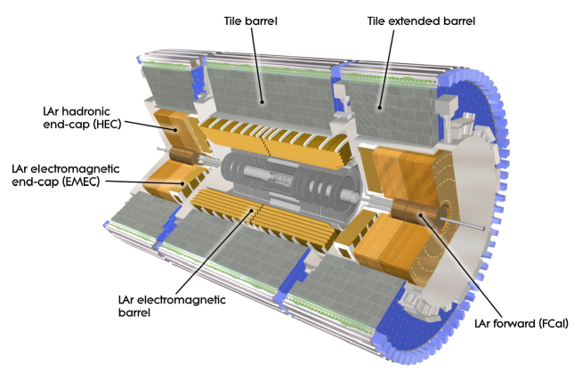
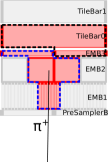
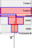
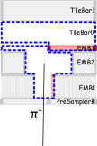
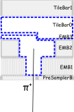
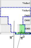
The calorimeters provide hermetic azimuthal coverage in the range . The detailed structure of the calorimeters within the tracker acceptance strongly influences the development of the shower subtraction algorithm described in this paper. In the central barrel region of the detector, a high-granularity liquid-argon (LAr) electromagnetic calorimeter with lead absorbers is surrounded by a hadronic sampling calorimeter (Tile) with steel absorbers and active scintillator tiles. The same LAr technology is used in the calorimeter endcaps, with fine granularity and lead absorbers for the EM endcap (EMEC), while the hadronic endcap (HEC) utilises copper absorbers with reduced granularity. The solid angle coverage is completed with forward copper/LAr and tungsten/LAr calorimeter modules (FCal) optimised for electromagnetic and hadronic measurements respectively. Figure 1 shows the physical location of the different calorimeters. To achieve a high spatial resolution, the calorimeter cells are arranged in a projective geometry with fine segmentation in and . Additionally, each of the calorimeters is longitudinally segmented into multiple layers, capturing the shower development in depth. In the region , a presampler detector is used to correct for the energy lost by electrons and photons upstream of the calorimeter. The presampler consists of an active LAr layer of thickness () in the barrel (endcap) region. The granularity of all the calorimeter layers within the tracker acceptance is given in Table 1.
The EM calorimeter is over 22 radiation lengths in depth, ensuring that there is little leakage of EM showers into the hadronic calorimeter. The total depth of the complete calorimeter is over 9 interaction lengths in the barrel and over 10 interaction lengths in the endcap, such that good containment of hadronic showers is obtained. Signals in the MS are used to correct the jet energy if the hadronic shower is not completely contained. In both the EM and Tile calorimeters, most of the absorber material is in the second layer. In the hadronic endcap, the material is more evenly spread between the layers.
| EM LAr calorimeter | ||||
|---|---|---|---|---|
| Barrel | Endcap | |||
| Presampler | ||||
| PreSamplerB/E | ||||
| 1st layer | ||||
| EMB1/EME1 | ||||
| 2nd layer | ||||
| EMB2/EME2 | ||||
| 3rd layer | ||||
| EMB3/EME3 | ||||
| Tile calorimeter | ||||
| Barrel | Extended barrel | |||
| 1st layer | ||||
| TileBar0/TileExt0 | ||||
| 2nd layer | ||||
| TileBar1/TileExt1 | ||||
| 3rd layer | ||||
| TileBar2/TileExt2 | ||||
| Hadronic LAr calorimeter | ||||
| Endcap | ||||
| 1st layer | ||||
| HEC0 | ||||
| 2nd layer | ||||
| HEC1 | ||||
| 3rd layer | ||||
| HEC2 | ||||
| 4th layer | ||||
| HEC3 | ||||
The muon spectrometer surrounds the calorimeters and is based on three large air-core toroid superconducting magnets with eight coils each. The field integral of the toroids ranges from to across most of the detector. It includes a system of precision tracking chambers and fast detectors for triggering.
3 Simulated event samples
A variety of MC samples are used in the optimisation and performance evaluation of the particle flow algorithm. The simplest samples consist of a single charged pion generated with a uniform spectrum in the logarithm of the generated pion energy and in the generated . Dijet samples generated with Pythia 8 (v8.160) [24, 25], with parameter values set to the ATLAS AU2 tune [26] and the CT10 parton distribution functions (PDF) set [27], form the main samples used to derive the jet energy scale and determine the jet energy resolution in simulation. The dijet samples are generated with a series of jet thresholds applied to the leading jet, reconstructed from all stable final-state particles excluding muons and neutrinos, using the anti- algorithm [28] with radius parameter 0.6 using FastJet (v3.0.3) [29, 30].
For comparison with collision data, events are generated with Powheg-Box (r1556) [31] using the CT10 PDF and are showered with Pythia 8, with the ATLAS AU2 tune. Additionally, top quark pair production is simulated with MC@NLO (v4.03) [32, 33] using the CT10 PDF set, interfaced with Herwig (v6.520) [34] for parton showering, and the underlying event is modelled by Jimmy (v4.31) [35]. The top quark samples are normalised using the cross-section calculated at next-to-next-to-leading order (NNLO) in QCD including resummation of next-to-next-to-leading logarithmic soft gluon terms with top++2.0 [36, 37, 38, 39, 40, 41, 42, 43], assuming a top quark mass of . Single-top-quark production processes contributing to the distributions shown are also simulated, but their contributions are negligible.
3.1 Detector simulation and pile-up modelling
All samples are simulated using Geant4 [44] within the ATLAS simulation framework [45] and are reconstructed using the noise threshold criteria used in 2012 data-taking [3]. Single-pion samples are simulated without pile-up, while dijet samples are simulated under three conditions: with no pile-up; with pile-up conditions similar to those in the 2012 data; and with a mean number of interactions per bunch crossing , where follows a Poisson distribution. In 2012, the mean value of was and the actual number of interactions per bunch crossing ranged from around 10 to 35 depending on the luminosity. The bunch spacing was . When compared to data, the MC samples are reweighted to have the same distribution of as present in the data. In all the samples simulated including pile-up, effects from both the same bunch crossing and previous/subsequent crossings are simulated by overlaying additional generated minimum-bias events on the hard-scatter event prior to reconstruction. The minimum-bias samples are generated using Pythia 8 with the ATLAS AM2 tune [46] and the MSTW2009 PDF set [47], and are simulated using the same software as the hard-scatter event.
3.2 Truth calorimeter energy and tracking information
For some samples the full Geant4 hit information [44] is retained for each calorimeter cell such that the true amount of hadronic and electromagnetic energy deposited by each generated particle is known. Only the measurable hadronic and electromagnetic energy deposits are counted, while the energy lost due to nuclear capture and particles escaping from the detector is not included. For a given charged pion the sum of these hits in a given cluster originating from this particle is denoted by .
Reconstructed topo-cluster energy is assigned to a given truth particle according to the proportion of Geant4 hits supplied to that topo-cluster by that particle. Using the Geant4 hit information in the inner detector a track is matched to a generated particle based on the fraction of hits on the track which originate from that particle [48].
4 Data sample
Data acquired during the period from March to December 2012 with the LHC operating at a centre-of-mass energy of are used to evaluate the level of agreement between data and Monte Carlo simulation of different outputs of the algorithm. Two samples with a looser preselection of events are reconstructed using the particle flow algorithm. A tighter selection is then used to evaluate its performance.
First, a enhanced sample is extracted from the 2012 dataset by selecting events containing two reconstructed muons [49], each with and , where the invariant mass of the dimuon pair is greater than , and the of the dimuon pair is greater than .
Similarly, a sample enhanced in events is obtained from events with an isolated muon and at least one hadronic jet which is required to be identified as a jet containing -hadrons (-jet). Events are selected that pass single-muon triggers and include one reconstructed muon satisfying , , for which the sum of additional track momenta in a cone of size around the muon track is less than . Additionally, a reconstructed calorimeter jet is required to be present with , , and pass the working point of the MV1 -tagging algorithm [50].
For both datasets, all ATLAS subdetectors are required to be operational with good data quality. Each dataset corresponds to an integrated luminosity of . To remove events suffering from significant electronic noise issues, cosmic rays or beam background, the analysis excludes events that contain calorimeter jets with which fail to satisfy the ?looser? ATLAS jet quality criteria [51, 52].
5 Topological clusters
The lateral and longitudinal segmentation of the calorimeters permits three-dimensional reconstruction of particle showers, implemented in the topological clustering algorithm [3]. Topo-clusters of calorimeter cells are seeded by cells whose absolute energy measurements exceed the expected noise by four times its standard deviation. The expected noise includes both electronic noise and the average contribution from pile-up, which depends on the run conditions. The topo-clusters are then expanded both laterally and longitudinally in two steps, first by iteratively adding all adjacent cells with absolute energies two standard deviations above noise, and finally adding all cells neighbouring the previous set. A splitting step follows, separating at most two local energy maxima into separate topo-clusters. Together with the ID tracks, these topo-clusters form the basic inputs to the particle flow algorithm.
The topological clustering algorithm employed in ATLAS is not designed to separate energy deposits from different particles, but rather to separate continuous energy showers of different nature, i.e. electromagnetic and hadronic, and also to suppress noise. The cluster-seeding threshold in the topo-clustering algorithm results in a large fraction of low-energy particles being unable to seed their own clusters. For example, in the central barrel of charged pions do not seed their own cluster [9].
While the granularity, noise thresholds and employed technologies vary across the different ATLAS calorimeters, they are initially calibrated to the electromagnetic scale (EM scale) to give the same response for electromagnetic showers from electrons or photons. Hadronic interactions produce responses that are lower than the EM scale, by amounts depending on where the showers develop. To account for this, the mean ratio of the energy deposited by a particle to the momentum of the particle is determined based on the position of the particle’s shower in the detector, as described in Section 6.4.
A local cluster (LC) weighting scheme is used to calibrate hadronic clusters to the correct scale [3]. Further development is needed to combine this with particle flow; therefore, in this work the topo-clusters used in the particle flow algorithm are calibrated at the EM scale.
6 Particle flow algorithm
A cell-based energy subtraction algorithm is employed to remove overlaps between the momentum and energy measurements made in the inner detector and calorimeters, respectively. Tracking and calorimetric information is combined for the reconstruction of hadronic jets and soft activity (additional hadronic recoil below the threshold used in jet reconstruction) in the event. The reconstruction of the soft activity is important for the calculation of the missing transverse momentum in the event [53], whose magnitude is denoted by .
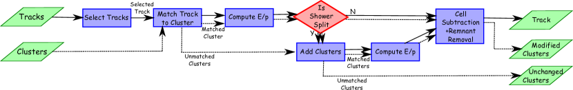
The particle flow algorithm provides a list of tracks and a list of topo-clusters containing both the unmodified topo-clusters and a set of new topo-clusters resulting from the energy subtraction procedure. This algorithm is sketched in Figure 2. First, well-measured tracks are selected following the criteria discussed in Section 6.2. The algorithm then attempts to match each track to a single topo-cluster in the calorimeter (Section 6.3). The expected energy in the calorimeter, deposited by the particle that also created the track, is computed based on the topo-cluster position and the track momentum (Section 6.4). It is relatively common for a single particle to deposit energy in multiple topo-clusters. For each track/topo-cluster system, the algorithm evaluates the probability that the particle energy was deposited in more than one topo-cluster. On this basis it decides if it is necessary to add more topo-clusters to the track/topo-cluster system to recover the full shower energy (Section 6.5). The expected energy deposited in the calorimeter by the particle that produced the track is subtracted cell by cell from the set of matched topo-clusters (Section 6.6). Finally, if the remaining energy in the system is consistent with the expected shower fluctuations of a single particle’s signal, the topo-cluster remnants are removed (Section 6.7).
This procedure is applied to tracks sorted in descending -order, firstly to the cases where only a single topo-cluster is matched to the track, and then to the other selected tracks. This methodology is illustrated in Figure 3.
| Track/topo-cluster | Split shower | Cell subtraction | Remnant removal | |
| matching | recovery | |||
|
|
|
|
|
 |
 |
 |
 |
|
 |
|
 |
 |
|
 |
|
 |
 |
Details about each step of the procedure are given in the rest of this section. After some general discussion of the properties of topo-clusters in the calorimeter, the energy subtraction procedure for each track is described. The procedure is accompanied by illustrations of performance metrics used to validate the configuration of the algorithm. The samples used for the validation are single-pion and dijet MC samples without pile-up, as described in the previous section. Charged pions dominate the charged component of the jet, which on average makes up two-thirds of the visible jet energy [54, 55]. Another quarter of the jet energy is contributed by photons from neutral hadron decays, and the remainder is carried by neutral hadrons that reach the calorimeter. Because the majority of tracks are generated by charged pions [56], particularly at low , the pion mass hypothesis is assumed for all tracks used by the particle flow algorithm to reconstruct jets. Likewise the energy subtraction is based on the calorimeter’s response to charged pions.
In the following sections, the values for the parameter set and the performance obtained for the 2012 dataset are discussed. These parameter values are not necessarily the product of a full optimisation, but it has been checked that the performance is not easily improved by variations of these choices. Details of the optimisation are beyond the scope of the paper.
6.1 Containment of showers within a single topo-cluster
The performance of the particle flow algorithm, especially the shower subtraction procedure, strongly relies on the topological clustering algorithm. Hence, it is important to quantify the extent to which the clustering algorithm distinguishes individual particles’ showers and how often it splits a single particle’s shower into more than one topo-cluster. The different configurations of topo-clusters containing energy from a given single pion are classified using two variables.
For a given topo-cluster , the fraction of the particle’s true energy contained in the topo-cluster (see Section 3.2), with respect to the total true energy deposited by the particle in all clustered cells, is defined as
| (3) |
where is the true energy deposited in topo-cluster by the generated particle under consideration and is the true energy deposited in all topo-clusters by that truth particle. For each particle, the topo-cluster with the highest value of is designated the leading topo-cluster, for which . The minimum number of topo-clusters needed to capture at least of the particle’s true energy, i.e. such that , is denoted by .
Topo-clusters can contain contributions from multiple particles, affecting the ability of the subtraction algorithm to separate the energy deposits of different particles. The purity for a topo-cluster is defined as the fraction of true energy within the topo-cluster which originates from the particle of interest:
| (4) |
For the leading topo-cluster, defined by having the highest , the purity value is denoted by .
Only charged particles depositing significant energy (at least of their true energy) in clustered cells are considered in the following plots, as in these cases there is significant energy in the calorimeter to remove. This also avoids the case where insufficient energy is present in any cell to form a cluster, which happens frequently for very low-energy particles [3].
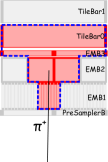
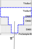
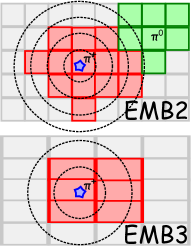
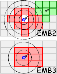
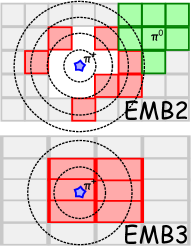
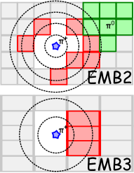
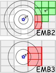
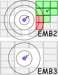
Figure 3 illustrates how the subtraction procedure is designed to deal with cases of different complexity. Four different scenarios are shown covering cases where the charged pion deposits its energy in one cluster, in two clusters, and where there is a nearby neutral pion which either deposits its energy in a separate cluster or the same cluster as the charged pion.
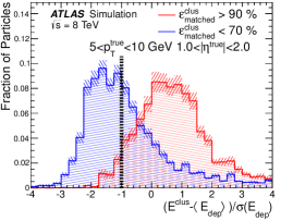
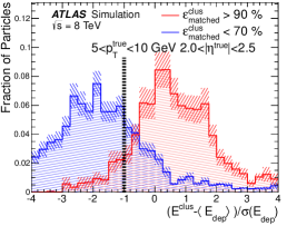
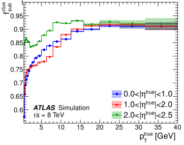
Several distributions are plotted for the dijet sample in which the energy of the leading jet, measured at truth level, is in the range . The distribution of is shown in Figure 4 for different and bins. It can be seen that decreases as the of the particle increases and very little dependence on is observed. Figure 5 shows the distribution of . As expected, increases with particle . It is particularly interesting to know the fraction of particles for which at least of the true energy is contained in a single topo-cluster () and this is shown in Figure 6. Lastly, Figure 7 shows the distribution of . This decreases as increases and has little dependence on .
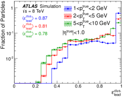
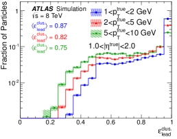
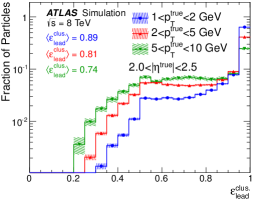
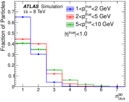
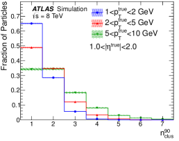
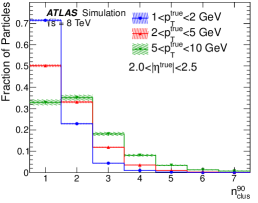
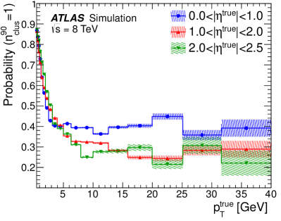
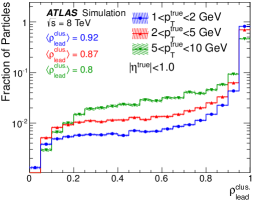
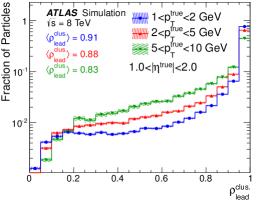
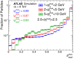
For more than of particles with , the shower is entirely contained within a single topo-cluster (). This fraction falls rapidly with particle , reaching for particles in the range . For particles with , of the particle energy can be captured within two topo-clusters in of cases. The topo-cluster purity also falls as the pion increases, with the target particle only contributing between and of the topo-cluster energy when . This is in part due to the tendency for high- particles to be produced in dense jets, while softer particles from the underlying event tend to be isolated from nearby activity.
In general, the subtraction of the hadronic shower is easier for cases with topo-clusters with high , and high , since in this configuration the topo-clustering algorithm has separated out the contributions from different particles.
6.2 Track selection
Tracks are selected which pass stringent quality criteria: at least nine hits in the silicon detectors are required, and tracks must have no missing Pixel hits when such hits would be expected [57]. This selection is designed such that the number of badly measured tracks is minimised and is referred to as ?tight selection?. No selection cuts are made on the association to the hard scatter vertex at this stage Additionally, tracks are required to be within and have . These criteria remain efficient for tracks from particles which are expected to deposit energy below the threshold needed to seed a topo-cluster or particles that do not reach the calorimeter. Including additional tracks by reducing the requirement to leads to a substantial increase in computing time without any corresponding improvement in jet resolution. This is due to their small contribution to the total jet .
Tracks with are excluded from the algorithm, as such energetic particles are often poorly isolated from nearby activity, compromising the accurate removal of the calorimeter energy associated with the track. In such cases, with the current subtraction scheme, there is no advantage in using the tracker measurement. This requirement was tuned both by monitoring the effectiveness of the energy subtraction using the true energy deposited in dijet MC events, and by measuring the jet resolution in MC simulation. The majority of tracks in jets with between 40 and 60 GeV have below 40 GeV, as shown later in Section 11.
In addition, any tracks matched to candidate electrons [58] or muons [49], without any isolation requirements, identified with medium quality criteria, are not selected and therefore are not considered for subtraction, as the algorithm is optimised for the subtraction of hadronic showers. The energy deposited in the calorimeter by electrons and muons is hence taken into account in the particle flow algorithm and any resulting topo-clusters are generally left unsubtracted.
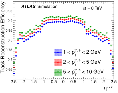
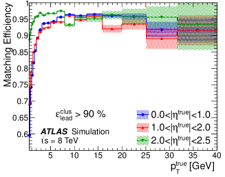
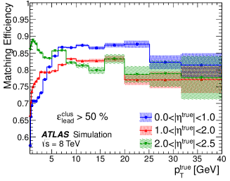
Figure 8 shows the charged-pion track reconstruction efficiency, for the tracks selected with the criteria described above, as a function of and in the dijet MC sample, with leading jets in the range and with similar pile-up to that in the 2012 data. The Monte Carlo generator information is used to match the reconstructed tracks to the generated particles [48]. The application of the tight quality criteria substantially reduces the rate of poorly measured tracks, as shown in Figure 9. Additionally, using the above selection, the fraction of combinatorial fake tracks arising from combining ID hits from different particles is negligible [48].
.
.
6.3 Matching tracks to topo-clusters
To remove the calorimeter energy where a particle has formed a single topo-cluster, the algorithm first attempts to match each selected track to one topo-cluster. The distances and between the barycentre of the topo-cluster and the track, extrapolated to the second layer of the EM calorimeter, are computed for each topo-cluster. The topo-clusters are ranked based on the distance metric
| (5) |
where and represent the angular topo-cluster widths, computed as the standard deviation of the displacements of the topo-cluster’s constituent cells in and with respect to the topo-cluster barycentre. This accounts for the spatial extent of the topo-clusters, which may contain energy deposits from multiple particles.
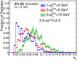
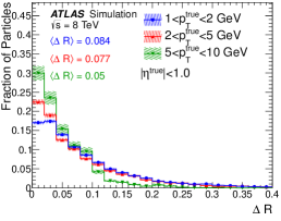
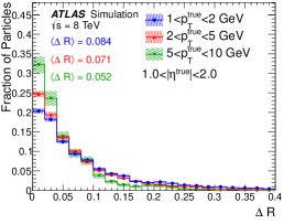
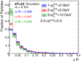
The distributions of and for single-particle samples are shown in Figure 10. The structure seen in these distributions is related to the calorimeter geometry. Each calorimeter layer has a different cell granularity in both dimensions, and this sets the minimum topo-cluster size. In particular, the granularity is significantly finer in the electromagnetic calorimeter, thus particles that primarily deposit their energy in either the electromagnetic and hadronic calorimeters form distinct populations. High-energy showers typically spread over more cells, broadening the corresponding topo-clusters. If the computed value of or is smaller than 0.05, it is set to 0.05.
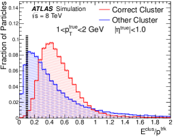
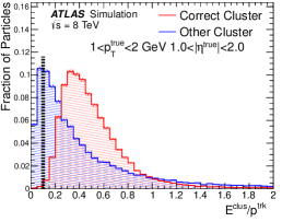
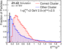
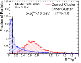
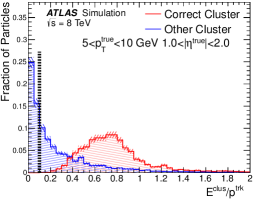
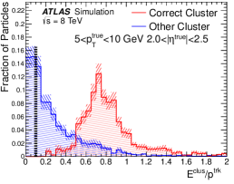
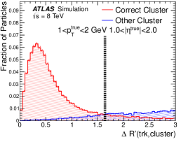
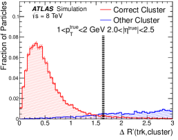
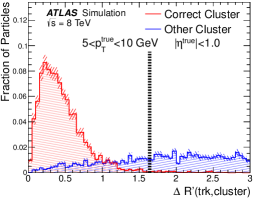
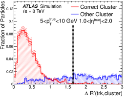
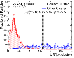
A preliminary selection of topo-clusters to be matched to the tracks is performed by requiring that , where is the energy of the topo-cluster and is the track momentum. The distribution of for the topo-cluster with at least of the true energy from the particle matched to the track – the “correct" one to match to – and for the closest other topo-cluster in is shown in Figure 11. For very soft particles, it is common that the closest other topo-cluster carries comparable to (although smaller than) the correct topo-cluster. About of incorrect topo-clusters are rejected by the cut for particles with . The difference in becomes much more pronounced for particles with , for which there is a very clear separation between the correct and incorrect topo-cluster matches, resulting in a 30– rejection rate for the incorrect topo-clusters. This is because at lower clusters come from both signal and electronic or pile-up noise. Furthermore, the particle spectrum is peaked towards lower values, and thus higher- topo-clusters are rarer. The requirement rejects the correct cluster for far less than of particles.
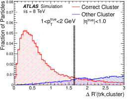
Next, an attempt is made to match the track to one of the preselected topo-clusters using the distance metric defined in Eq. 5. The distribution of between the track and the topo-cluster with of the truth particle energy and to the closest other preselected topo-cluster is shown in Figure 12 for the dijet MC sample. From this figure, it is seen that the correct topo-cluster almost always lies at a small relative to other clusters. Hence, the closest preselected topo-cluster in is taken to be the matched topo-cluster. This criterion selects the correct topo-cluster with a high probability, succeeding for virtually all particles with . If no preselected topo-cluster is found in a cone of size , it is assumed that this particle did not form a topo-cluster in the calorimeter. In such cases the track is retained in the list of tracks and no subtraction is performed. The numerical value corresponds to a one-sided Gaussian confidence interval of , and has not been optimised. However, as seen in Figure 12, this cone size almost always includes the correct topo-cluster, while rejecting the bulk of incorrect clusters.
6.4 Evaluation of the expected deposited particle energy through determination
It is necessary to know how much energy a particle with measured momentum deposits on average, given by , in order to correctly subtract the energy from the calorimeter for a particle whose track has been reconstructed. The expectation value (which is also a measure of the mean response) is determined using single-particle samples without pile-up by summing the energies of topo-clusters in a cone of size 0.4 around the track position, extrapolated to the second layer of the EM calorimeter. This cone size is large enough to entirely capture the energy of the majority of particle showers. This is also sufficient in dijet events, as demonstrated in Figure 13, where one might expect the clusters to be broader due to the presence of other particles. The subscript ?ref? is used here and in the following to indicate values determined from single-pion samples.
Variations in due to detector geometry and shower development are captured by binning the measurement in the and of the track as well as the layer of highest energy density (LHED), defined in the next section. The LHED is also used to determine the order in which cells are subtracted in subsequent stages of the algorithm.
The spread of the expected energy deposition, denoted by , is determined from the standard deviation of the distribution in single-pion samples. It is used in order to quantify the consistency of the measured with the expectation from in both the split-shower recovery (Section 6.5) and remnant removal (Section 6.7).
6.4.1 Layer of highest energy density
The dense electromagnetic shower core has a well-defined ellipsoidal shape in –. It is therefore desirable to locate this core, such that the energy subtraction may be performed first in this region before progressing to the less regular shower periphery. The LHED is taken to be the layer which shows the largest rate of increase in energy density, as a function of the number of interaction lengths from the front face of the calorimeter. This is determined as follows:
-
•
The energy density is calculated for the th cell in the th layer of the calorimeter as
(6) with being the energy in and the volume of the cell expressed in radiation lengths. The energy measured in the Presampler is added to that of the first layer in the EM calorimeter. In addition, the Tile and HEC calorimeters are treated as single layers. Thus, the procedure takes into account four layers – three in the EM calorimeter and one in the hadronic calorimeter. Only cells in the topo-clusters matched to the track under consideration are used.
-
•
Cells are then weighted based on their proximity to the extrapolated track position in the layer, favouring cells that are closer to the track and hence more likely to contain energy from the selected particle. The weight for each cell, , is computed from the integral over the cell area in – of a Gaussian distribution centred on the extrapolated track position with a width in of 0.035, similar to the Molière radius of the LAr calorimeter.
-
•
A weighted average energy density for each layer is calculated as
(7) -
•
Finally, the rate of increase in in each layer is determined. Taking to be the depth of layer in interaction lengths, the rate of increase is defined as
(8) where the values and are assigned, and the first calorimeter layer has the index .
The layer for which is maximal is identified as the LHED.
6.5 Recovering split showers
Particles do not always deposit all their energy in a single topo-cluster, as seen in Figure 5. Clearly, handling the multiple topo-cluster case is crucial, particularly the two topo-cluster case, which is very common. The next stages of the algorithm are therefore firstly to determine if the shower is split across several clusters, and then to add further clusters for consideration when this is the case.
The discriminant used to distinguish the single and multiple topo-cluster cases is the significance of the difference between the expected energy and that of the matched topo-cluster (defined using the algorithm in Section 6.3),
| (9) |
The distribution of is shown in Figure 14 for two categories of matched topo-clusters: those with and those with . A clear difference is observed between the distributions for the two categories, demonstrating the separation between showers that are and are not contained in a single cluster. More than of clusters with have . Based on this observation a split shower recovery procedure is run if : topo-clusters within a cone of around the track position extrapolated to the second EM calorimeter layer are considered to be matched to the track. As can be seen in the figure, the split shower recovery procedure is typically run of the time when . The full set of matched clusters is then considered when the energy is subtracted from the calorimeter.
6.6 Cell-by-cell subtraction
Once a set of topo-clusters corresponding to the track has been selected, the subtraction step is executed. If exceeds the total energy of the set of matched topo-clusters, then the topo-clusters are simply removed. Otherwise, subtraction is performed cell by cell.
Starting from the extrapolated track position in the LHED, a parameterised shower shape is used to map out the most likely energy density profile in each layer. This profile is determined from a single MC sample and is dependent on the track momentum and pseudorapidity, as well as on the LHED for the set of considered topo-clusters. Rings are formed in , space around the extrapolated track. The rings are just wide enough to always contain at least one calorimeter cell, independently of the extrapolated position, and are confined to a single calorimeter layer. Rings within a single layer are equally spaced in radius. The average energy density in each ring is then computed, and the rings are ranked in descending order of energy density, irrespective of which layer each ring is in. Subtraction starts from the ring with the highest energy density (the innermost ring of the LHED) and proceeds successively to the lower-density rings. If the energy in the cells in the current ring is less than the remaining energy required to reach , these cells are simply removed and the energy still to be subtracted is reduced by the total energy of the ring. If instead the ring has more energy than is still to be removed, each cell in the ring is scaled down in energy by the fraction needed to reach the expected energy from the particle, then the process halts. Figure 15 shows a cartoon of how this subtraction works, removing cells in different rings from different layers until the expected energy deposit is reached.
6.7 Remnant removal
If the energy remaining in the set of cells and/or topo-clusters that survive the energy subtraction is consistent with the width of the distribution, specifically if this energy is less than , it is assumed that the topo-cluster system was produced by a single particle. The remnant energy therefore originates purely from shower fluctuations and so the energy in the remaining cells is removed. Conversely, if the remaining energy is above this threshold, the remnant topo-cluster(s) are retained – it being likely that multiple particles deposited energy in the vicinity. Figure 16 shows how this criterion is able to separate cases where the matched topo-cluster has true deposited energy only from a single particle from those where there are multiple contributing particles.
After this final step, the set of selected tracks and the remaining topo-clusters in the calorimeter together should ideally represent the reconstructed event with no double counting of energy between the subdetectors.
7 Performance of the subtraction algorithm at truth level
The performance of each step of the particle flow algorithm is evaluated exploiting the detailed energy information at truth level available in Monte Carlo generated events. For these studies a dijet sample with leading truth jet between 20 and without pile-up is used.
7.1 Track–cluster matching performance
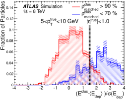
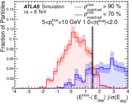
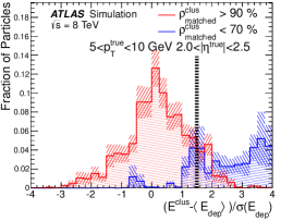
Initially, the algorithm attempts to match the track to a single topo-cluster containing the full particle energy. Figure 17 shows the fraction of tracks whose matched cluster has or . When almost all of the deposited energy is contained within a single topo-cluster, the probability to match a track to this topo-cluster (matching probability) is above in all regions, for particles with . The matching probability falls to between and when up to half the particle’s energy is permitted to fall in other topo-clusters. Due to changes in the calorimeter geometry, the splitting rate and hence the matching probability vary significantly for particles in different pseudorapidity regions. In particular, the larger cell size at higher enhances the likelihood of capturing soft particle showers in a single topo-cluster, as seen in Figures 4 and 5, which results in the matching efficiency increasing at low for .
7.2 Split-shower recovery performance
Frequently, a particle’s energy is not completely contained within the single best-match topo-cluster, in which case the split shower recovery procedure is applied. The effectiveness of the recovery can be judged based on whether the procedure is correctly triggered, and on the extent to which the energy subtraction is improved by its execution.
Figure 18 shows the fraction of the true deposited energy contained within the matched topo-cluster, separately for cases where the split shower recovery procedure is and is not triggered, as determined by the criteria described in Section 6.5. In the cases where the split shower recovery procedure is not run, is found to be high, confirming that the comparison of topo-cluster energy and is successfully identifying good topo-cluster matches. Conversely, the split shower recovery procedure is activated when is low, particularly for higher- particles, which are expected to split their energy between multiple topo-clusters more often. Furthermore, as the particle rises, the width of the calorimeter response distribution decreases, making it easier to distinguish the different cases.
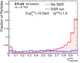

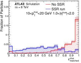
Figure 19 shows the fraction of the true deposited energy of the pions considered for subtraction, in the set of clusters matched to the track, as a function of true . For particles with , with split shower recovery active, is greater than on average. The subtraction algorithm misses more energy for softer showers, which are harder to capture completely. While could be increased by simply attempting recovery more frequently, expanding the topo-cluster matching procedure in this fashion increases the risk of incorrectly subtracting neutral energy; hence the split shower recovery procedure cannot be applied indiscriminately. The settings used in the studies presented in this paper are a reasonable compromise between these two cases.
7.3 Accuracy of cell subtraction
The cell subtraction procedure removes the expected calorimeter energy contribution based on the track properties. It is instructive to identify the energy that is incorrectly subtracted from the calorimeter, to properly understand and optimise the performance of the algorithm.
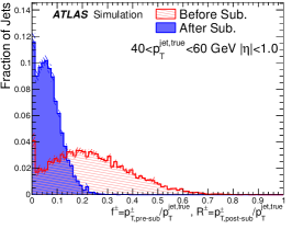
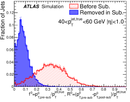
Truth particles are assigned reconstructed energy in topo-clusters as described in Section 3.2, and then classified depending on whether or not a track was reconstructed for the particle. The reconstructed energy assigned to each particle is computed both before subtraction and after the subtraction has been performed, using the remaining cells. In the ideal case, the subtraction should remove all the energy in the calorimeter assigned to stable truth particles which have reconstructed tracks, and should not remove any energy assigned to other particles. The total transverse momentum of clusters associated with particles in a truth jet where a track was reconstructed before (after) subtraction is defined as . Similarly, the transverse momentum of clusters associated with the other particles in a truth jet, neutral particles and those that did not create selected, reconstructed tracks, before (after) subtraction as . The corresponding transverse momentum fractions are defined as ().
Three measures are established, to quantify the degree to which the energy is incorrectly subtracted. The incorrectly subtracted fractions for the two classes of particles are:
| (10) |
and
| (11) |
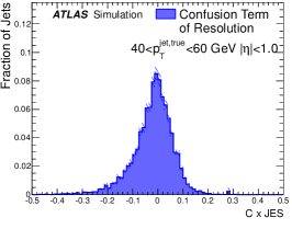
such that corresponds to the fraction of surviving momentum associated with particles where the track measurement is used, which should have been removed, while gives the fraction of momentum removed that should have been retained as it is associated with particles where the calorimeter measurement is being used. These two variables are combined into the confusion term
| (12) |
which is equivalent to the net effect of both mistakes on the final jet transverse momentum, as there is a potential cancellation between the two effects. An ideal subtraction algorithm would give zero for all three quantities.
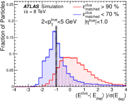
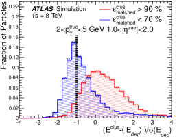
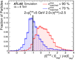
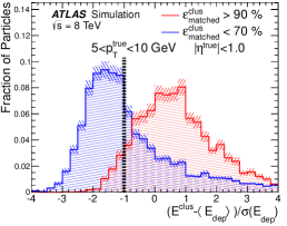
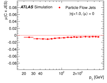
Figure 20 shows the fractions associated with the different classes of particle, before and after the subtraction algorithm has been executed for jets with a true energy in the range . The confusion term is also shown, multiplied by the jet energy scale factor that would be applied to these reconstructed jets, such that its magnitude () is directly comparable to the reconstructed jet resolution.
Clearly, the subtraction does not perform perfectly, but most of the correct energy is removed – the mean value of the confusion is , with an RMS of . The slight bias towards negative values suggests that the subtraction algorithm is more likely to remove additional neutral energy rather than to miss charged energy and the RMS gives an indication of the contribution from this confusion to the overall jet resolution.
Figure 21 shows as a function of . The mean value of the JES weighted confusion remains close to zero and always within , showing that on average the algorithm removes the correct amount of energy from the calorimeter. The RMS decreases with increasing . This is due to a combination of the particle spectrum becoming harder, such that the efficiency of matching to the correct cluster increases; the increasing difficulty of subtracting the hadronic showers in the denser environments of high- jets; and the fact that no subtraction is performed for tracks above , resulting in the fraction of the jet considered for subtraction decreasing with increasing jet .
7.4 Visualising the subtraction
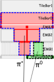
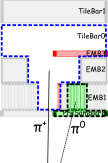
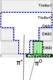
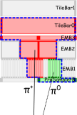
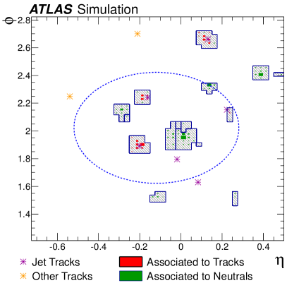
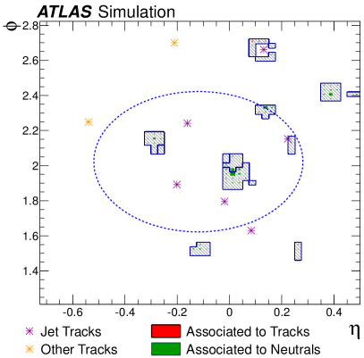
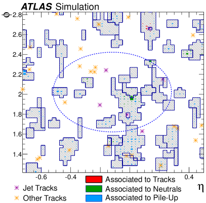
For a concrete demonstration of successes and failures of the subtraction algorithm, it is instructive to look at a specific event in the calorimeter. Figure 22 illustrates the action of the algorithm in the second layer of the EM calorimeter, where the majority of low-energy showers are contained. The focus is on a region where a truth jet is present. In general, the subtraction works well in the absence of pile-up, as the two topo-clusters inside the jet radius with energy mainly associated with charged particles at truth level are entirely removed. Nevertheless, examples can be seen where small mistakes are made. For example, the algorithm additionally removes some cells containing neutral-particle energy from the topo-cluster just above the track at .
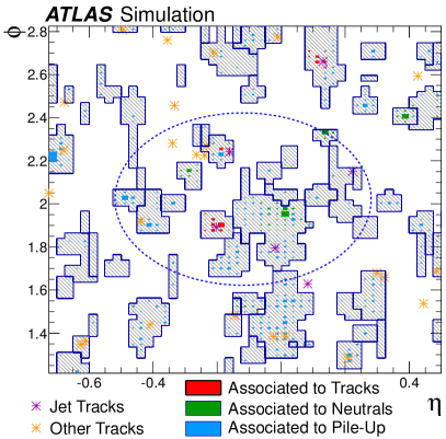
The figure also shows the same event, overlaid with pile-up corresponding to . Pile-up contributions are identified by subtracting the energy reconstructed without pile-up and are illustrated in blue. The pile-up supplies many more energy deposits and tracks within the region under scrutiny. However, the subtraction continues to function effectively, removing energy in the vicinity of pile-up tracks and hence the post-subtraction cell distribution more closely resembles that without pile-up, especially inside the jet radius. Because tracks classified as originating from pile-up are ignored in jet reconstruction (see Section 8), the jet energy after subtraction is mainly contaminated by neutral pile-up contributions.
8 Jet reconstruction and calibration
Improved jet performance is the primary goal of using particle flow reconstruction. Particle flow jets are reconstructed using the anti- algorithm with radius parameter 0.4. The inputs to jet reconstruction are the ensemble of positive energy topo-clusters surviving the energy subtraction step and the selected tracks that are matched to the hard-scatter primary vertex. These tracks are selected by requiring , where is the distance of closest approach of the track to the hard-scatter primary vertex along the -axis. This criterion retains the tracks from the hard scatter, while removing a large fraction of the tracks (and their associated calorimeter energy) from pile-up interactions [59]. Prior to jet-finding, the topo-cluster and are recomputed with respect to the hard-scatter primary vertex position, rather than the detector origin.
Calorimeter jets are similarly reconstructed using the anti- algorithm with radius parameter 0.4, but take as input topo-clusters calibrated at the LC-scale, uncorrected for the primary vertex position. For the purposes of jet calibration, truth jets are formed from stable final-state particles excluding muons and neutrinos, using the anti- algorithm with radius parameter 0.4.333 ?Stable particles? are defined as those with proper lifetimes longer than .
8.1 Overview of particle flow jet calibration
Calibration of these jets closely follows the scheme used for standard calorimeter jets described in Refs. [4, 5, 6, 7] and is carried out over the range . The reconstructed jets are first corrected for pile-up contamination using the jet ghost-area subtraction method [60, 61]. This is described in Section 8.2. A numerical inversion [6] based on Monte Carlo events (see Section 8.3) restores the jet response to match the average response at particle level. Additional fluctuations in jet response are corrected for using a global sequential correction process [4], which is detailed in Section 8.4. No in situ correction to data is applied in the context of these studies; however, the degree of agreement between data and MC simulation is checked using the balance of jets against a boson decaying to two muons.
The features of particle flow jet calibration that differ from the calibration of calorimeter jets are discussed below, and results from the different stages of the jet calibration are shown.
8.2 Area-based pile-up correction
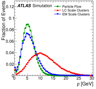
The calorimeter jet pile-up correction uses a transverse energy density calculated from topo-clusters using jets [62, 63], for a correction of the form of multiplied by the area of the jet [61]. For particle flow jets, the transverse energy density therefore needs to be computed using charged and neutral particle flow objects to correctly account for the differences in the jet constituents. As discussed above, the tracks associated to pile-up vertices are omitted, eliminating a large fraction of the energy deposits from charged particles from pile-up interactions. The jet-area subtraction therefore corrects for the impact of charged underlying-event hadrons, charged particles from out-of-time interactions, and more importantly, neutral particles from pile-up interactions. This correction is evaluated prior to calibration of the jet energy scale. Figure 23 shows the distribution of the median transverse energy density in dijet MC events for particle flow objects and for topo-clusters. The topo-cluster is calculated with the ensemble of clusters, calibrated either at the EM scale or LC scale, and the particle flow jets use topo-clusters calibrated at the EM scale.
The LC-scale energy density is larger than the EM-scale energy density due to the application of the cell weights to calibrate cells to the hadronic scale. Compared to the EM- and LC-scale energy densities, has a lower per-event value for particle flow jets in 2012 conditions, due to the reduced pile-up contribution. The removal of the charged particle flow objects that are not associated with the hard-scatter primary vertex more than compensates for the higher energy scale for charged hadrons from the underlying event.
8.3 Monte Carlo numerical inversion
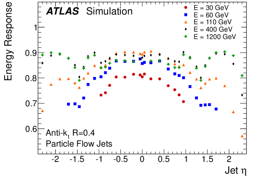
Figure 24 shows the energy response prior to the MC-based jet energy scale correction. The same numerical procedure as described in LABEL:\cite[cite]{[\@@bibref{}{ATLAS-CONF-2015-037}{}{}]} is applied and successfully corrects for the hadron response, at a similar level to that observed in LABEL:\cite[cite]{[\@@bibref{}{ATLAS-CONF-2015-037}{}{}]}.
8.4 Global sequential correction
The numerical inversion calibration restores the average reconstructed jet energy to the mean value of the truth jet energy, accounting for variations in the jet response due to the jet energy and pseudorapidity. However, other jet characteristics such as the flavour of the originating parton and the composition of the hadrons created in jet fragmentation may cause further differences in the response. A global sequential correction [4] that makes use of additional observables adapts the jet energy calibration to account for such variations, thereby improving the jet resolution without changing the scale. The variables used for particle flow jets are not the same as those used for calorimeter jets, as tracks have already been used in the calculation of the energy of the jet constituents.
As the name implies, the corrections corresponding to each variable are applied consecutively. Three variables are used as inputs to the correction:
-
1.
the fraction of the jet energy measured from constituent tracks (charged fraction), i.e. those tracks associated to the jet;
-
2.
the fraction of jet energy measured in the third EM calorimeter layer;
-
3.
the fraction of jet energy measured in the first Tile calorimeter layer.
The first of these variables allows the degree of under-calibrated signal, due to the lower energy deposit of hadrons in the hadronic calorimeter, to be determined. The calorimeter-layer energy fractions allow corrections to be made for the energy lost in dead material between the LAr and Tile calorimeters.
8.5 In situ validation of JES
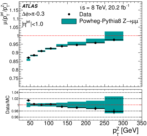
A full in situ calibration and evaluation of the uncertainties on the JES [64] is not performed for these studies. However, to confirm that the ATLAS MC simulation describes the particle flow jet characteristics well enough to reproduce the jet energy scale in data, similar methods are used to validate the jet calibration. A sample of events with a jet balancing the boson is used for the validation. A preselection is made using the criteria described in Section 4. The particle flow algorithm is run on these events and further requirements, discussed below, are applied. The jet with the highest (j1) and the reconstructed boson are required to be well separated in azimuthal angle, . Events with any additional jet within , with or , are vetoed, where j2 denotes the jet with the second highest . In Figure 25, the mean value of the ratio of the transverse momentum of the jet to that of the boson is shown for data and MC simulation for jets with . The mean value is determined using a Gaussian fit to the distribution in bins of the -boson . The double-ratio of data to MC simulation is also shown. The simulation reproduces the data to within , and in general is consistent with the data points within statistical uncertainties. At high the data/MC ratio is expected to tend towards that of the calorimeter jets [6, 7], as a large fraction of the jet’s energy is carried by particles above the cut made on the track momentum. For > 200 GeV it is observed that the jet energy scale of calorimeter jets in data is typically below that in simulation.
9 Resolution of jets in Monte Carlo simulation
The largest expected benefit from using the particle flow reconstruction as input to jet-finding is an improvement of the jet energy and angular resolution for low- jets. In this section, the jet resolution achieved with particle flow methods is compared with that attained using standard calorimeter jet reconstruction.
9.1 Transverse momentum resolution
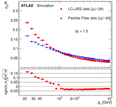
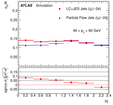
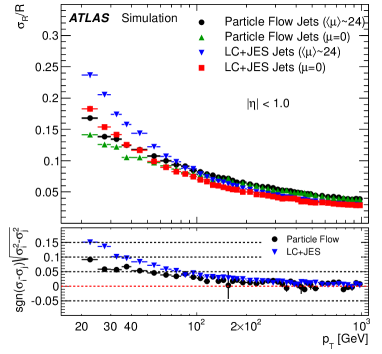
In Figure 26, the relative jet transverse momentum resolution for particle flow and calorimeter jets is shown as a function of jet transverse momentum for jets in the pseudorapidity range , and as a function of for jets with . Particle flow jets are calibrated using the procedures described in Section 8, while calorimeter jets use the more detailed procedure described in Refs. [4, 5, 6, 7]. The particle flow jets perform better than calorimeter jets at transverse momenta of up to in the central region, benefiting from the improved scale for low- hadrons and intrinsic pile-up suppression (elaborated on in Section 10). However, at high transverse momenta, the particle flow reconstruction performs slightly worse than the standard reconstruction. This is due to two effects. The dense core of a jet poses a challenge to tracking algorithms, causing the tracking efficiency and accuracy to degrade in high- jets. Furthermore, the close proximity of the showers within the jet increases the degree of confusion during the cell subtraction stage. To counteract this, the track used for particle flow reconstruction is required to be for the 2012 data. Alternative solutions, such as smoothly disabling the algorithm for individual tracks as the particle environment becomes more dense, are expected to restore the particle flow jet performance to match that of the calorimeter jets at high energies. The benefits of particle flow also diminish toward the more forward regions as the cell granularity decreases, as shown in Figure 26(b)
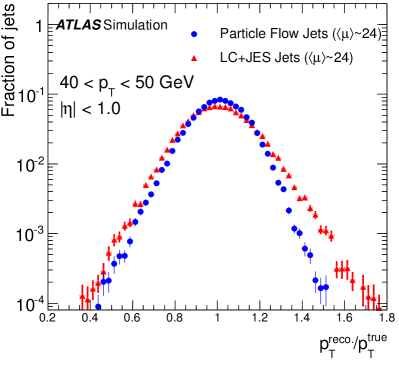
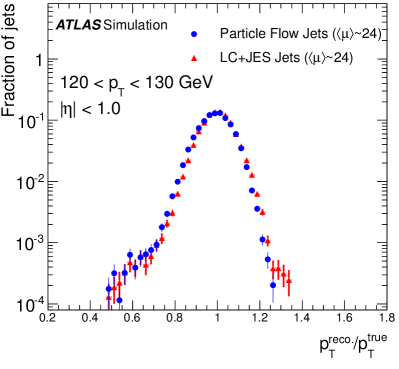
In Figure 27, the underlying distributions of the ratio of reconstructed to true are shown for two different jet bins. This demonstrates that the particle flow algorithm does not introduce significant tails in the response at either low or high . The low-side tail visible in Figure 27(b) is present in both calorimeter and particle flow jets and is caused by dead material and inactive detector regions.
9.2 Angular resolution of jets
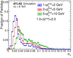
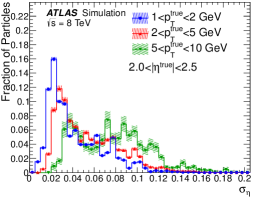
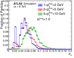
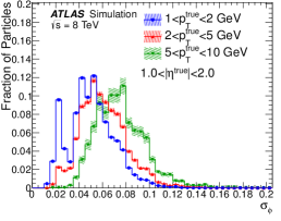
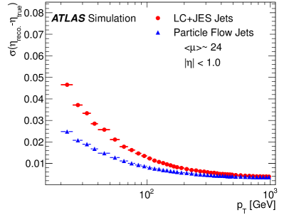
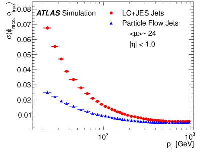
Besides improving the resolution of jets, the particle flow algorithm is expected to improve the angular () resolution of jets. This is due to three different effects. Firstly, usage of tracks to measure charged particles results in a much better angular resolution for individual particles than that obtained using topo-clusters, because the tracker’s angular resolution is far superior to that of the calorimeter. Secondly, the track four-momentum can be determined at the perigee, before the charged particles have been spread out by the magnetic field, thereby improving the resolution for the jet. Thirdly, the suppression of charged pile-up particles should also reduce mismeasurements of the jet direction.
Figure 28 shows the angular resolution in and as a function of the reconstructed jet transverse momentum for particle flow and calorimeter jets. It is determined from the standard deviation of a Gaussian fit over to the difference between the and values for the reconstructed and matched truth () jets in the central region. At low , where the three effects described above are expected to be more important, significant improvements are seen in both the and resolutions. It is interesting to note that for particle flow jets the and resolutions are similar, while for calorimeter jets the resolution is worse due to the aforementioned effect of the magnetic field on charged particles.
10 Effect of pile-up on the jet resolution and rejection of pile-up jets
At the design luminosity of the LHC, and even in 2012 data-taking conditions, in- and out-of-time pile-up contribute significantly to the signals measured in the ATLAS detector, increasing the fluctuations in jet energy measurements. The pile-up suppression inherent in the particle flow reconstruction and the calibration of charged particles through the use of tracks significantly mitigates the degradation of jet resolution from pile-up and eliminates jets reconstructed from pile-up deposits, making the particle flow method a powerful tool, especially as the LHC luminosity increases.
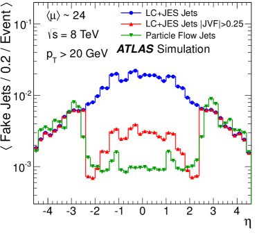
10.1 Pile-up jet rate
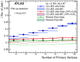
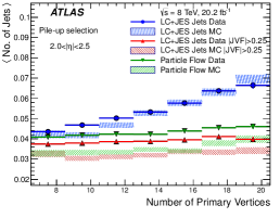
In the presence of pile-up, jets can arise from particles not produced in the hard-scatter interaction. These jets are here referred to as ?fake jets?. Figure 29(a) shows the fake-jet rate as a function of the jet for particle flow jets compared to calorimeter jets with and without track-based pile-up suppression [65]. These rates are evaluated using a dijet MC sample overlaid with simulated minimum-bias events approximating the data-taking conditions in 2012. The jet vertex fraction (JVF) is defined as the ratio of two scalar sums of track momenta: the numerator is the scalar sum of the of tracks that originate from the hard-scatter primary vertex and are associated with the jet; the denominator is the scalar sum of the transverse momenta of all tracks associated with that jet.444Jets with no tracks associated with them are assigned . Within the tracker coverage of , the fake rate for particle flow jets drops by an order of magnitude compared to the standard calorimeter jets. The small increase in the rate of particle flow fake jets around is related to the worse performance of the particle flow algorithm in the transition region between the barrel and extended barrel of the Tile calorimeter, which is significantly affected by pile-up contributions [3].
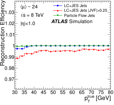
For , the jets are virtually identical, and hence the fake rate shows no differences. This rejection rate is comparable to that achieved using the JVF discriminant, which can likewise only be applied within the tracker coverage. Here, the comparison is made to a threshold of 0.25 for calorimeter jets, which is not as powerful as the particle flow fake-jet rate reduction. The inefficiency of the particle flow jet-finding is negligible, as can be seen from Figure 29(b). In contrast, the inefficiency generated by requiring is clearly visible (it should be noted that in 2012 JVF cuts were only applied to calorimeter jets up to a of ). Below , the jet resolution causes some reconstructed jets to fall below the jet reconstruction energy threshold so these values are not shown.
A more detailed study of the pile-up jet rates is carried out in a sample, both in data and MC simulation, by isolating several phase-space regions that are enriched in hard-scatter or pile-up jets. A preselection is made using the criteria described in Section 4. The particle flow algorithm is run on these events and further requirements are applied: events are selected with two isolated muons, each with , with invariant mass and , ensuring that the boson recoils against hadronic activity. Figure 30 displays two regions of phase space: one opposite the recoiling boson, where large amounts of hard-scatter jet activity are expected, and one off-axis, which is more sensitive to pile-up jet activity.

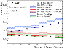
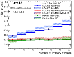
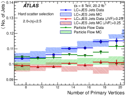
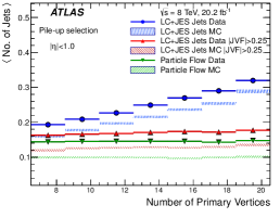
Figure 31 shows the average number of jets with in the hard-scatter-enriched region for different ranges as a function of the number of primary vertices. The distributions are stable for particle flow jets and for calorimeter jets with as a function the number of primary vertices in all regions. The only exception is in the region, where in Figure 29 a slight increase in the jet fake rate is visible for jet pseudorapidities very close to the tracker boundary. This is due to the jet area collecting charged-particle pile-up contributions that are outside the ID acceptance. If the JVF cut is not applied to the calorimeter jets, the jet multiplicity grows with increasing pile-up. Figure 32 shows that in the pile-up-enriched selection, the particle flow and calorimeter jets with a JVF selection still show no dependence on the number of reconstructed vertices in all regions. The observed difference between data and MC simulation for both jet collections is due to a poor modelling of this region of phase space. These distributions establish the high stability of particle flow jets in varying pile-up conditions.
10.2 Pile-up effects on jet energy resolution
In addition to simply suppressing jets from pile-up, the particle flow procedure reduces the fluctuations in the jet energy measurements due to pile-up contributions. This is demonstrated by Figure 33, which compares the jet energy resolution for particle flow and calorimeter jets with and without pile-up. Even in the absence of pile-up, the particle flow jets have a better resolution at values below . With pile-up conditions similar to those in the 2012 data, the cross-over point is at , indicating that particle flow reconstruction alleviates a significant contribution from pile-up even for fairly energetic jets. The direct effect of pile-up can be seen in the lower panel, where the difference in quadrature between the resolutions with and without pile-up is shown. The origin of the increase in the resolution with pile-up is discussed in detail in LABEL:\cite[cite]{[\@@bibref{}{ATLAS-CONF-2015-037}{}{}]}. It is shown that additional energy deposits are the primary cause of the degradation of the calorimeter jet resolution. This effect is mitigated by the particle flow algorithm in two ways. Firstly, the subtraction of topo-clusters formed by charged particles from pile-up vertices prior to jet-finding eliminates a major source of fluctuations. Secondly, the increase in the constituent scale of hard-scatter jets from the use of calibrated tracks, rather than energy clusters in the calorimeter, amplifies the signal, effectively suppressing the contribution from pile-up. This second mechanism is found to be the main contributing factor.
For jets, the total jet resolution without pile-up is . Referring back to Figure 20(c), confusion contributes to the jet resolution in the absence of pile-up. Since the terms are combined in quadrature, confusion contributes significantly to the overall jet resolution, although it does not totally dominate. While additional confusion can be caused by the presence of pile-up particles, the net effect is that pile-up affects the resolution of particle flow jets less than that of calorimeter jets.
11 Comparison of data and Monte Carlo simulation
It is crucial that the quantities used by the particle flow reconstruction are accurately described by the ATLAS detector simulation. In this section, particle flow jet properties are compared for and events in data and MC simulation. Various observables are validated, from low-level jet characteristics to derived observables relevant to physics analyses.
11.1 Individual jet properties
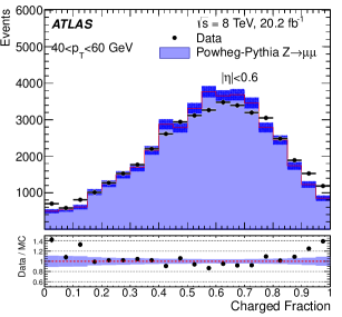
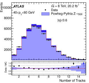
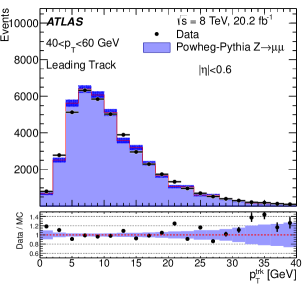
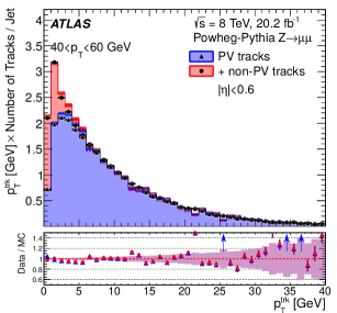
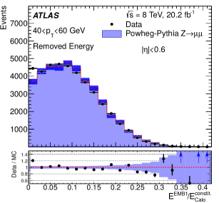
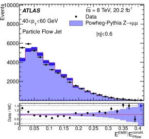
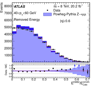
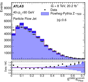
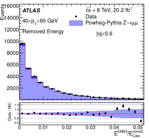
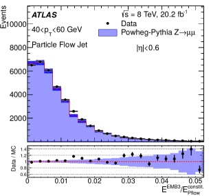
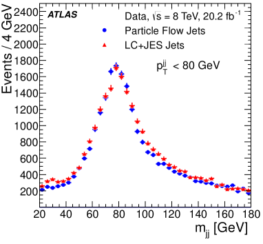
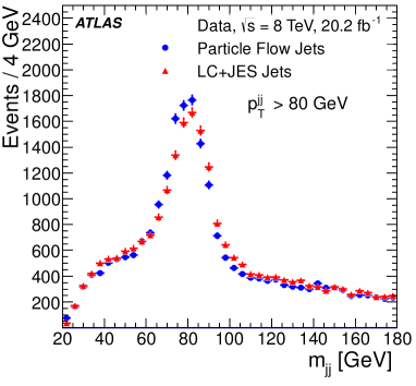
A sample of jets is selected in events, as in Section 8, and used for a comparison between data and MC simulation. As the subtraction takes place at the cell level, the energy subtracted from each layer of the calorimeter demonstrates how well the subtraction procedure is modelled. To determine the energy before subtraction the particle flow jets are matched to jets formed solely from topo-clusters at the electromagnetic scale. A similar selection to that used to evaluate the jet energy scale is used. The leading jet is required to be opposite a reconstructed boson decaying to two muons with . The of the reconstructed boson is required to be above and the reconstructed jets must have . Figures 34 and 35 show the properties of central jets. The MC simulation describes the data reasonably well for the jet track multiplicity, fraction of the jet carried by tracks as well as the amount of subtracted or surviving energy in each layer of the EM barrel. Similar levels of agreement are observed for jets in the endcap regions of the detector.
11.2 Event-level observables
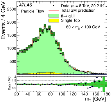
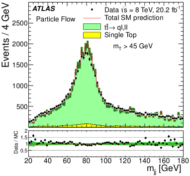
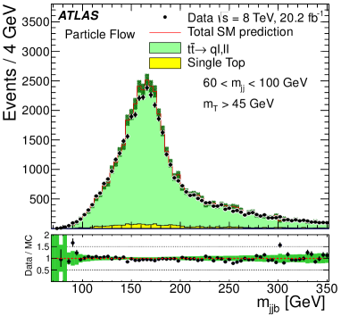
Finally, the particle flow performance is examined in a sample of selected events; a sample triggered by a single-muon trigger with a single offline reconstructed muon is used. At least four jets with and are required and two of these are required to have been -tagged using the MV1 algorithm and have and .555As the -tagging algorithm has only been calibrated for calorimeter jets, the particle flow jets use the calorimeter jet information from the closest jet in in order to decide if the jet is -tagged. This selects a pure sample of events. The event is reconstructed from the vector sum of the calibrated jets with , the muon and all remaining tracks associated with the hard-scatter primary vertex but not associated with these objects. This is then used to form the transverse mass variable defined by . The invariant mass of the two leading non--tagged jets, , forms a hadronic candidate, while the invariant masses of each of the two -tagged jets and these two non--tagged jets form two hadronic top quark candidates, .
Figure 36 compares the data with MC simulation for these three variables; and . The MC simulation describes the data very well in all three distributions. Figure 37 shows the distribution for particle flow jets compared to the distribution obtained from the same selection applied to calorimeter jets (with ). For the calorimeter jet selection, the is reconstructed from the muon, jets, photons and remaining unassociated clusters [53]. The two selections are applied separately; hence the exact numbers of events in the plots differ. The particle flow reconstruction provides a good measure and narrower width of the peak for both low and high . Gaussian fits to the data in the range give widths of and for particle flow reconstruction and that based on calorimeter jets, respectively, for . For , the widths were found to be and , respectively. At very high values of , the gains would further diminish (see Figure 26).
12 Conclusions
The particle flow algorithm used by the ATLAS Collaboration for of collisions at at the LHC is presented. This algorithm aims to accurately subtract energy deposited by tracks in the calorimeter, exploiting the good calorimeter granularity and longitudinal segmentation. Use of particle flow leads to improved energy and angular resolution of jets compared to techniques that only use the calorimeter in the central region of the detector.
In 2012 data-taking conditions, the transverse momentum resolution of particle flow jets calibrated with a global sequential correction is superior up to for . For a representative jet of , the resolution is improved from the resolution of calorimeter jets with local cluster weighting calibration to . Jet angular resolutions are improved across the entire spectrum, with and decreasing from 0.03 to 0.02 and 0.05 to 0.02, respectively, for a jet of .
Rejection of charged particles from pile-up interactions in jet reconstruction leads to substantially better jet resolution and to the suppression of jets due to pile-up interactions by an order of magnitude within the tracker acceptance, with negligible inefficiency for jets from the hard-scatter interaction. This outperforms a purely track-based jet pile-up discriminant typically used in ATLAS analyses, which achieves similar pile-up suppression at the cost of about one percent in hard-scatter jet efficiency.
The algorithm therefore achieves a better performance for hadronic observables such as reconstructed resonant particle masses.
Studies which compare data with MC simulation demonstrate that jet properties used for energy measurement and calibration are modelled well by the ATLAS simulation, both before and after application of the particle flow algorithm. This translates to good agreement between data and simulation for derived physics observables, such as invariant masses of combinations of jets.
The algorithm has been integrated into the ATLAS software framework for Run 2 of the LHC. As demonstrated, it is robust against pile-up and should therefore perform well under the conditions encountered in Run 2.
Acknowledgements
We thank CERN for the very successful operation of the LHC, as well as the support staff from our institutions without whom ATLAS could not be operated efficiently.
We acknowledge the support of ANPCyT, Argentina; YerPhI, Armenia; ARC, Australia; BMWFW and FWF, Austria; ANAS, Azerbaijan; SSTC, Belarus; CNPq and FAPESP, Brazil; NSERC, NRC and CFI, Canada; CERN; CONICYT, Chile; CAS, MOST and NSFC, China; COLCIENCIAS, Colombia; MSMT CR, MPO CR and VSC CR, Czech Republic; DNRF and DNSRC, Denmark; IN2P3-CNRS, CEA-DSM/IRFU, France; SRNSF, Georgia; BMBF, HGF, and MPG, Germany; GSRT, Greece; RGC, Hong Kong SAR, China; ISF, I-CORE and Benoziyo Center, Israel; INFN, Italy; MEXT and JSPS, Japan; CNRST, Morocco; NWO, Netherlands; RCN, Norway; MNiSW and NCN, Poland; FCT, Portugal; MNE/IFA, Romania; MES of Russia and NRC KI, Russian Federation; JINR; MESTD, Serbia; MSSR, Slovakia; ARRS and MIZŠ, Slovenia; DST/NRF, South Africa; MINECO, Spain; SRC and Wallenberg Foundation, Sweden; SERI, SNSF and Cantons of Bern and Geneva, Switzerland; MOST, Taiwan; TAEK, Turkey; STFC, United Kingdom; DOE and NSF, United States of America. In addition, individual groups and members have received support from BCKDF, the Canada Council, CANARIE, CRC, Compute Canada, FQRNT, and the Ontario Innovation Trust, Canada; EPLANET, ERC, ERDF, FP7, Horizon 2020 and Marie Skłodowska-Curie Actions, European Union; Investissements d’Avenir Labex and Idex, ANR, Région Auvergne and Fondation Partager le Savoir, France; DFG and AvH Foundation, Germany; Herakleitos, Thales and Aristeia programmes co-financed by EU-ESF and the Greek NSRF; BSF, GIF and Minerva, Israel; BRF, Norway; CERCA Programme Generalitat de Catalunya, Generalitat Valenciana, Spain; the Royal Society and Leverhulme Trust, United Kingdom.
The crucial computing support from all WLCG partners is acknowledged gratefully, in particular from CERN, the ATLAS Tier-1 facilities at TRIUMF (Canada), NDGF (Denmark, Norway, Sweden), CC-IN2P3 (France), KIT/GridKA (Germany), INFN-CNAF (Italy), NL-T1 (Netherlands), PIC (Spain), ASGC (Taiwan), RAL (UK) and BNL (USA), the Tier-2 facilities worldwide and large non-WLCG resource providers. Major contributors of computing resources are listed in Ref. [66].
References
- [1] Lyndon Evans and Philip Bryant “LHC Machine” In JINST 3, 2008, pp. S08001 DOI: 10.1088/1748-0221/3/08/S08001
- [2] ATLAS Collaboration “The ATLAS Experiment at the CERN Large Hadron Collider” In JINST 3, 2008, pp. S08003 DOI: 10.1088/1748-0221/3/08/S08003
- [3] ATLAS Collaboration “Topological cell clustering in the ATLAS calorimeters and its performance in LHC Run 1” In Submitted to Eur. Phys. J. C, 2016 arXiv:1603.02934 [hep-ex]
- [4] ATLAS Collaboration “Jet global sequential corrections with the ATLAS detector in proton–proton collisions at ”, ATLAS-CONF-2015-002, 2015 URL: https://cds.cern.ch/record/2001682
- [5] ATLAS Collaboration “Data-driven determination of the energy scale and resolution of jets reconstructed in the ATLAS calorimeters using dijet and multijet events at ”, ATLAS-CONF-2015-017, 2015 URL: https://cds.cern.ch/record/2008678
- [6] ATLAS Collaboration “Monte Carlo Calibration and Combination of In-situ Measurements of Jet Energy Scale, Jet Energy Resolution and Jet Mass in ATLAS”, ATLAS-CONF-2015-037, 2015 URL: https://cds.cern.ch/record/2044941
- [7] ATLAS Collaboration “Determination of the jet energy scale and resolution at ATLAS using -jet events in data at ”, ATLAS-CONF-2015-057, 2015 URL: https://cds.cern.ch/record/2059846
- [8] ATLAS Collaboration “ATLAS: Detector and physics performance technical design report. Volume 1”, 1999 URL: https://cds.cern.ch/record/391176
- [9] ATLAS Collaboration “A measurement of single hadron response using data at with the ATLAS detector”, ATL-PHYS-PUB-2014-002, 2014 URL: https://cds.cern.ch/record/1668961
- [10] ALEPH Collaboration and D. Buskulic “Performance of the ALEPH detector at LEP” In Nucl. Instrum. Meth. A 360.CERN-PPE-94-170. FSU-SCRI-95-70, 1994, pp. 481–506. 44 p DOI: 10.1016/0168-9002(95)00138-7
- [11] M. Peez “Search for deviations from the Standard Model in high transverse energy processes at the electron-proton collider HERA”, DESY-THESIS-2003-023, 2003 URL: http://www-h1.desy.de/psfiles/theses/h1th-317.pdf
- [12] ZEUS Collaboration and J. Breitweg “Measurement of the diffractive structure function at HERA” In Eur. Phys. J C 1, 1998, pp. 81 DOI: 10.1007/s100520050063
- [13] ZEUS Collaboration and J. Breitweg “Measurement of the Diffractive Cross Section in Deep Inelastic Scattering using ZEUS 1994 Data” In Eur. Phys. J. C 6, 1999, pp. 43–66 DOI: 10.1007/s100529801016
- [14] P. Abreu “Performance of the DELPHI detector” In Nucl. Instrum. Meth. A 378, 1996, pp. 57–100 DOI: 10.1016/0168-9002(96)00463-9
- [15] CDF Collaboration and A. Abulencia “Measurement of in collisions at ” In Phys. Rev. D 75, 2007, pp. 092004 DOI: 10.1103/PhysRevD.75.092004
- [16] DØ Collaboration and V. M. Abazov “Measurement of at ” In Phys. Lett. B 670.4–5, 2009, pp. 292–299 DOI: 10.1016/j.physletb.2008.11.010
- [17] ATLAS Collaboration “Reconstruction of hadronic decay products of tau leptons with the ATLAS experiment” In Eur. Phys. J. C 76, 2016, pp. 295 DOI: 10.1140/epjc/s10052-016-4110-0
- [18] CMS Collaboration “Particle-Flow Event Reconstruction in CMS and Performance for Jets, Taus, and MET”, CMS-PAS-PFT-09-001, 2009
- [19] CMS Collaboration “Commissioning of the Particle-flow Event Reconstruction with the first LHC collisions recorded in the CMS detector”, CMS-PAS-PFT-10-001, 2010
- [20] CMS Collaboration “Determination of Jet Energy Calibration and Transverse Momentum Resolution in CMS” In JINST 6, 2011, pp. P11002 DOI: 10.1088/1748-0221/6/11/P11002
- [21] M. A. Thomson “Particle Flow Calorimetry and the PandoraPFA Algorithm” In Nucl. Instrum. Meth. A 611, 2009, pp. 25–40 DOI: 10.1016/j.nima.2009.09.009
- [22] C. Adloff et al. “Tests of a particle flow algorithm with CALICE test beam data” In JINST 6, 2011, pp. P07005 DOI: 10.1088/1748-0221/6/07/P07005
- [23] ATLAS Collaboration “Alignment of the ATLAS Inner Detector and its Performance in 2012”, ATLAS-CONF-2014-047, 2014 URL: https://cds.cern.ch/record/1741021
- [24] Torbjorn Sjöstrand, Stephen Mrenna and Peter Z. Skands “A Brief Introduction to PYTHIA 8.1” In Comput. Phys. Commun. 178, 2008, pp. 852–867 DOI: 10.1016/j.cpc.2008.01.036
- [25] R. Corke and T. Sjöstrand “Improved Parton Showers at Large Transverse Momenta” In Eur. Phys. J. C 69, 2010, pp. 1–18 DOI: 10.1140/epjc/s10052-010-1409-0
- [26] ATLAS Collaboration “Summary of ATLAS Pythia 8 tunes”, ATL-PHYS-PUB-2012-003, 2012 URL: https://cds.cern.ch/record/1474107
- [27] H.-L. Lai “New parton distributions for collider physics” In Phys. Rev. D 82, 2010, pp. 074024 DOI: 10.1103/PhysRevD.82.074024
- [28] Matteo Cacciari, Gavin P. Salam and Gregory Soyez “The anti- jet clustering algorithm” In JHEP 04, 2008, pp. 063 DOI: 10.1088/1126-6708/2008/04/063
- [29] Matteo Cacciari, Gavin P. Salam and Gregory Soyez URL: http://fastjet.fr
- [30] Matteo Cacciari and Gavin P. Salam “Dispelling the myth for the jet-finder” In Phys. Lett. B 641, 2006, pp. 57 DOI: 10.1016/j.physletb.2006.08.037
- [31] Paolo Nason “A new method for combining NLO QCD with shower Monte Carlo algorithms” In JHEP 11, 2004, pp. 040 DOI: 10.1088/1126-6708/2004/11/040
- [32] S. Frixione and B.R. Webber “Matching NLO QCD computations and parton shower simulations” In JHEP 06, 2002, pp. 029 DOI: 10.1088/1126-6708/2002/06/029
- [33] S. Frixione, P. Nason and B.R. Webber “Matching NLO QCD and parton showers in heavy flavour production” In JHEP 08, 2003, pp. 007 DOI: 10.1088/1126-6708/2003/08/007
- [34] G. Corcella “HERWIG 6: an event generator for hadron emission reactions with interfering gluons (including supersymmetric processes)” In JHEP 01, 2001, pp. 010 DOI: 10.1088/1126-6708/2001/01/010
- [35] J. M. Butterworth, Jeffrey R. Forshaw and M. H. Seymour “Multiparton interactions in photoproduction at HERA” In Z. Phys. C 72, 1996, pp. 637–646 DOI: 10.1007/s002880050286
- [36] M. Aliev et al. “HATHOR: HAdronic Top and Heavy quarks crOss section calculatoR” In Comput. Phys. Commun. 182, 2011, pp. 1034–1046 DOI: 10.1016/j.cpc.2010.12.040
- [37] M. Beneke, P. Falgari, S. Klein and C. Schwinn “Hadronic top-quark pair production with NNLL threshold resummation” In Nucl. Phys. B 855, 2012, pp. 695–741 DOI: 10.1016/j.nuclphysb.2011.10.021
- [38] Michal Czakon, Paul Fiedler and Alexander Mitov “The total top quark pair production cross-section at hadron colliders through O()” In Phys. Rev. Lett. 110, 2013, pp. 252004 DOI: 10.1103/PhysRevLett.110.252004
- [39] Michal Czakon and Alexander Mitov “NNLO corrections to top pair production at hadron colliders: the quark-gluon reaction” In JHEP 01, 2013, pp. 080 DOI: 10.1007/JHEP01(2013)080
- [40] Michal Czakon and Alexander Mitov “NNLO corrections to top-pair production at hadron colliders: the all-fermionic scattering channels” In JHEP 12, 2012, pp. 054 DOI: 10.1007/JHEP12(2012)054
- [41] Peter Bärnreuther, Michal Czakon and Alexander Mitov “Percent Level Precision Physics at the Tevatron: First Genuine NNLO QCD Corrections to ” In Phys. Rev. Lett. 109, 2012, pp. 132001 DOI: 10.1103/PhysRevLett.109.132001
- [42] Matteo Cacciari et al. “Top-pair production at hadron colliders with next-to-next-to-leading logarithmic soft-gluon resummation” In Phys. Lett. B 710, 2012, pp. 612–622 DOI: 10.1016/j.physletb.2012.03.013
- [43] Michal Czakon and Alexander Mitov “Top++: A Program for the Calculation of the Top-Pair Cross-Section at Hadron Colliders” In Comput. Phys. Commun. 185, 2014, pp. 2930 DOI: 10.1016/j.cpc.2014.06.021
- [44] S. Agostinelli “GEANT4: A simulation toolkit” In Nucl. Instrum. Meth. A 506, 2003, pp. 250–303 DOI: 10.1016/S0168-9002(03)01368-8
- [45] ATLAS Collaboration “The ATLAS Simulation Infrastructure” In Eur. Phys. J. C 70, 2010, pp. 823 DOI: 10.1140/epjc/s10052-010-1429-9
- [46] ATLAS Collaboration “ATLAS tunes of Pythia 6 and Pythia 8 for MC11”, ATL-PHYS-PUB-2011-009, 2011 URL: https://cds.cern.ch/record/1363300
- [47] A. Sherstnev and R. S. Thorne “Parton distributions for LO generators” In Eur. Phys. J. C 55, 2008, pp. 553 DOI: 10.1140/epjc/s10052-008-0610-x
- [48] ATLAS Collaboration “Charged-particle distributions in interactions measured with the ATLAS detector at the LHC” In Phys. Lett. B 758, 2016, pp. 67 DOI: 10.1016/j.physletb.2016.04.050
- [49] ATLAS Collaboration “Measurement of the muon reconstruction performance of the ATLAS detector using 2011 and 2012 LHC proton–proton collision data” In Eur. Phys. J. C 74, 2014, pp. 3130 DOI: 10.1140/epjc/s10052-014-3130-x
- [50] ATLAS Collaboration “Commissioning of the ATLAS high performance -tagging algorithms in the collision data”, ATLAS-CONF-2011-102, 2011 URL: https://cds.cern.ch/record/1369219
- [51] ATLAS Collaboration “Characterisation and mitigation of beam-induced backgrounds observed in the ATLAS detector during the 2011 proton–proton run” In JINST 8, 2013, pp. P07004 DOI: 10.1088/1748-0221/8/07/P07004
- [52] ATLAS Collaboration “Selection of jets produced in proton–proton collisions with the ATLAS detector using 2011 data”, ATLAS-CONF-2012-020, 2012 URL: https://cds.cern.ch/record/1430034
- [53] ATLAS Collaboration “Performance of algorithms that reconstruct missing transverse momentum in proton–proton collisions in the ATLAS detector”, 2016 arXiv:1609.09324 [hep-ex]
- [54] I. G. Knowles and G. D. Lafferty “Hadronization in decay” In J. Phys. G 23, 1997, pp. 731–789 DOI: 10.1088/0954-3899/23/7/003
- [55] M.G. Green, S.L Lloyd, P.N Ratoff and D.R Ward “Electron-Positron Physics at the Z”, Studies in high energy physics, cosmology, and gravitation Bristol: IOP Pub., 1998
- [56] ATLAS Collaboration “ measurement in the ATLAS Pixel Detector and its use for particle identification”, ATLAS-CONF-2011-016, 2011 URL: https://cds.cern.ch/record/1336519
- [57] ATLAS Collaboration “Performance of the ATLAS Inner Detector Track and Vertex Reconstruction in High Pile-Up LHC Environment”, ATLAS-CONF-2012-042, 2012 URL: https://cds.cern.ch/record/1435196
- [58] ATLAS Collaboration “Electron efficiency measurements with the ATLAS detector using 2012 LHC proton-proton collision data”, 2016 arXiv:1612.01456 [hep-ex]
- [59] ATLAS Collaboration “Charged-particle multiplicities in interactions at measured with the ATLAS detector at the LHC” In Phys. Lett. B 688, 2010, pp. 21 DOI: 10.1016/j.physletb.2010.03.064
- [60] Matteo Cacciari, Gavin P. Salam and Gregory Soyez “The Catchment Area of Jets” In JHEP 04, 2008, pp. 005 DOI: 10.1088/1126-6708/2008/04/005
- [61] M. Cacciari and G. P. Salam “Pileup subtraction using jet areas” In Phys. Lett. B 659, 2008, pp. 119–126 DOI: 10.1016/j.physletb.2007.09.077
- [62] Stephen D. Ellis and Davison E. Soper “Successive combination jet algorithm for hadron collisions” In Phys. Rev. D 48, 1993, pp. 3160–3166 DOI: 10.1103/PhysRevD.48.3160
- [63] S. Catani, Yuri L. Dokshitzer, M. H. Seymour and B. R. Webber “Longitudinally invariant clustering algorithms for hadron hadron collisions” In Nucl. Phys. B 406, 1993, pp. 187–224 DOI: 10.1016/0550-3213(93)90166-M
- [64] ATLAS Collaboration “Jet energy measurement and its systematic uncertainty in proton–proton collisions at with the ATLAS detector” In Eur. Phys. J. C 75, 2015, pp. 17 DOI: 10.1140/epjc/s10052-014-3190-y
- [65] ATLAS Collaboration “Performance of pile-up mitigation techniques for jets in collisions with the ATLAS detector” In Eur. Phys. J. C 76.11, 2016, pp. 581 DOI: 10.1140/epjc/s10052-016-4395-z
- [66] ATLAS Collaboration “ATLAS Computing Acknowledgements 2016–2017”, ATL-GEN-PUB-2016-002 URL: https://cds.cern.ch/record/2202407
The ATLAS Collaboration
M. Aaboud, G. Aad, B. Abbott, J. Abdallah, O. Abdinov,∗, B. Abeloos, S.H. Abidi, O.S. AbouZeid, N.L. Abraham, H. Abramowicz, H. Abreu, R. Abreu, Y. Abulaiti, B.S. Acharya,a, S. Adachi, L. Adamczyk, J. Adelman, M. Adersberger, T. Adye, A.A. Affolder, T. Agatonovic-Jovin, C. Agheorghiesei, J.A. Aguilar-Saavedra, S.P. Ahlen, F. Ahmadov,b, G. Aielli, S. Akatsuka, H. Akerstedt, T.P.A. Åkesson, A.V. Akimov, G.L. Alberghi, J. Albert, M.J. Alconada Verzini, M. Aleksa, I.N. Aleksandrov, C. Alexa, G. Alexander, T. Alexopoulos, M. Alhroob, B. Ali, M. Aliev, G. Alimonti, J. Alison, S.P. Alkire, B.M.M. Allbrooke, B.W. Allen, P.P. Allport, A. Aloisio, A. Alonso, F. Alonso, C. Alpigiani, A.A. Alshehri, M. Alstaty, B. Alvarez Gonzalez, D. Álvarez Piqueras, M.G. Alviggi, B.T. Amadio, Y. Amaral Coutinho, C. Amelung, D. Amidei, S.P. Amor Dos Santos, A. Amorim, S. Amoroso, G. Amundsen, C. Anastopoulos, L.S. Ancu, N. Andari, T. Andeen, C.F. Anders, J.K. Anders, K.J. Anderson, A. Andreazza, V. Andrei, S. Angelidakis, I. Angelozzi, A. Angerami, F. Anghinolfi, A.V. Anisenkov,c, N. Anjos, A. Annovi, C. Antel, M. Antonelli, A. Antonov,∗, D.J. Antrim, F. Anulli, M. Aoki, L. Aperio Bella, G. Arabidze, Y. Arai, J.P. Araque, V. Araujo Ferraz, A.T.H. Arce, R.E. Ardell, F.A. Arduh, J-F. Arguin, S. Argyropoulos, M. Arik, A.J. Armbruster, L.J. Armitage, O. Arnaez, H. Arnold, M. Arratia, O. Arslan, A. Artamonov, G. Artoni, S. Artz, S. Asai, N. Asbah, A. Ashkenazi, L. Asquith, K. Assamagan, R. Astalos, M. Atkinson, N.B. Atlay, K. Augsten, G. Avolio, B. Axen, M.K. Ayoub, G. Azuelos,d, A.E. Baas, M.J. Baca, H. Bachacou, K. Bachas, M. Backes, M. Backhaus, P. Bagiacchi, P. Bagnaia, H. Bahrasemani, J.T. Baines, M. Bajic, O.K. Baker, E.M. Baldin,c, P. Balek, T. Balestri, F. Balli, W.K. Balunas, E. Banas, Sw. Banerjee,e, A.A.E. Bannoura, L. Barak, E.L. Barberio, D. Barberis, M. Barbero, T. Barillari, M-S Barisits, T. Barklow, N. Barlow, S.L. Barnes, B.M. Barnett, R.M. Barnett, Z. Barnovska-Blenessy, A. Baroncelli, G. Barone, A.J. Barr, L. Barranco Navarro, F. Barreiro, J. Barreiro Guimarães da Costa, R. Bartoldus, A.E. Barton, P. Bartos, A. Basalaev, A. Bassalat,f, R.L. Bates, S.J. Batista, J.R. Batley, M. Battaglia, M. Bauce, F. Bauer, H.S. Bawa,g, J.B. Beacham, M.D. Beattie, T. Beau, P.H. Beauchemin, P. Bechtle, H.P. Beck,h, K. Becker, M. Becker, M. Beckingham, C. Becot, A.J. Beddall, A. Beddall, V.A. Bednyakov, M. Bedognetti, C.P. Bee, T.A. Beermann, M. Begalli, M. Begel, J.K. Behr, A.S. Bell, G. Bella, L. Bellagamba, A. Bellerive, M. Bellomo, K. Belotskiy, O. Beltramello, N.L. Belyaev, O. Benary,∗, D. Benchekroun, M. Bender, K. Bendtz, N. Benekos, Y. Benhammou, E. Benhar Noccioli, J. Benitez, D.P. Benjamin, M. Benoit, J.R. Bensinger, S. Bentvelsen, L. Beresford, M. Beretta, D. Berge, E. Bergeaas Kuutmann, N. Berger, J. Beringer, S. Berlendis, N.R. Bernard, G. Bernardi, C. Bernius, F.U. Bernlochner, T. Berry, P. Berta, C. Bertella, G. Bertoli, F. Bertolucci, I.A. Bertram, C. Bertsche, D. Bertsche, G.J. Besjes, O. Bessidskaia Bylund, M. Bessner, N. Besson, C. Betancourt, A. Bethani, S. Bethke, A.J. Bevan, R.M. Bianchi, O. Biebel, D. Biedermann, R. Bielski, N.V. Biesuz, M. Biglietti, J. Bilbao De Mendizabal, T.R.V. Billoud, H. Bilokon, M. Bindi, A. Bingul, C. Bini, S. Biondi, T. Bisanz, C. Bittrich, D.M. Bjergaard, C.W. Black, J.E. Black, K.M. Black, D. Blackburn, R.E. Blair, T. Blazek, I. Bloch, C. Blocker, A. Blue, W. Blum,∗, U. Blumenschein, S. Blunier, G.J. Bobbink, V.S. Bobrovnikov,c, S.S. Bocchetta, A. Bocci, C. Bock, M. Boehler, D. Boerner, D. Bogavac, A.G. Bogdanchikov, C. Bohm, V. Boisvert, P. Bokan,i, T. Bold, A.S. Boldyrev, M. Bomben, M. Bona, M. Boonekamp, A. Borisov, G. Borissov, J. Bortfeldt, D. Bortoletto, V. Bortolotto, K. Bos, D. Boscherini, M. Bosman, J.D. Bossio Sola, J. Boudreau, J. Bouffard, E.V. Bouhova-Thacker, D. Boumediene, C. Bourdarios, S.K. Boutle, A. Boveia, J. Boyd, I.R. Boyko, J. Bracinik, A. Brandt, G. Brandt, O. Brandt, U. Bratzler, B. Brau, J.E. Brau, W.D. Breaden Madden, K. Brendlinger, A.J. Brennan, L. Brenner, R. Brenner, S. Bressler, D.L. Briglin, T.M. Bristow, D. Britton, D. Britzger, F.M. Brochu, I. Brock, R. Brock, G. Brooijmans, T. Brooks, W.K. Brooks, J. Brosamer, E. Brost, J.H Broughton, P.A. Bruckman de Renstrom, D. Bruncko, A. Bruni, G. Bruni, L.S. Bruni, BH Brunt, M. Bruschi, N. Bruscino, P. Bryant, L. Bryngemark, T. Buanes, Q. Buat, P. Buchholz, A.G. Buckley, I.A. Budagov, F. Buehrer, M.K. Bugge, O. Bulekov, D. Bullock, H. Burckhart, S. Burdin, C.D. Burgard, A.M. Burger, B. Burghgrave, K. Burka, S. Burke, I. Burmeister, J.T.P. Burr, E. Busato, D. Büscher, V. Büscher, P. Bussey, J.M. Butler, C.M. Buttar, J.M. Butterworth, P. Butti, W. Buttinger, A. Buzatu, A.R. Buzykaev,c, S. Cabrera Urbán, D. Caforio, V.M. Cairo, O. Cakir, N. Calace, P. Calafiura, A. Calandri, G. Calderini, P. Calfayan, G. Callea, L.P. Caloba, S. Calvente Lopez, D. Calvet, S. Calvet, T.P. Calvet, R. Camacho Toro, S. Camarda, P. Camarri, D. Cameron, R. Caminal Armadans, C. Camincher, S. Campana, M. Campanelli, A. Camplani, A. Campoverde, V. Canale, M. Cano Bret, J. Cantero, T. Cao, M.D.M. Capeans Garrido, I. Caprini, M. Caprini, M. Capua, R.M. Carbone, R. Cardarelli, F. Cardillo, I. Carli, T. Carli, G. Carlino, B.T. Carlson, L. Carminati, R.M.D. Carney, S. Caron, E. Carquin, G.D. Carrillo-Montoya, J. Carvalho, D. Casadei, M.P. Casado,j, M. Casolino, D.W. Casper, R. Castelijn, A. Castelli, V. Castillo Gimenez, N.F. Castro,k, A. Catinaccio, J.R. Catmore, A. Cattai, J. Caudron, V. Cavaliere, E. Cavallaro, D. Cavalli, M. Cavalli-Sforza, V. Cavasinni, E. Celebi, F. Ceradini, L. Cerda Alberich, A.S. Cerqueira, A. Cerri, L. Cerrito, F. Cerutti, A. Cervelli, S.A. Cetin, A. Chafaq, D. Chakraborty, S.K. Chan, W.S. Chan, Y.L. Chan, P. Chang, J.D. Chapman, D.G. Charlton, A. Chatterjee, C.C. Chau, C.A. Chavez Barajas, S. Che, S. Cheatham, A. Chegwidden, S. Chekanov, S.V. Chekulaev, G.A. Chelkov,l, M.A. Chelstowska, C. Chen, H. Chen, S. Chen, S. Chen, X. Chen,m, Y. Chen, H.C. Cheng, H.J. Cheng, Y. Cheng, A. Cheplakov, E. Cheremushkina, R. Cherkaoui El Moursli, V. Chernyatin,∗, E. Cheu, L. Chevalier, V. Chiarella, G. Chiarelli, G. Chiodini, A.S. Chisholm, A. Chitan, Y.H. Chiu, M.V. Chizhov, K. Choi, A.R. Chomont, S. Chouridou, B.K.B. Chow, V. Christodoulou, D. Chromek-Burckhart, M.C. Chu, J. Chudoba, A.J. Chuinard, J.J. Chwastowski, L. Chytka, A.K. Ciftci, D. Cinca, V. Cindro, I.A. Cioara, C. Ciocca, A. Ciocio, F. Cirotto, Z.H. Citron, M. Citterio, M. Ciubancan, A. Clark, B.L. Clark, M.R. Clark, P.J. Clark, R.N. Clarke, C. Clement, Y. Coadou, M. Cobal, A. Coccaro, J. Cochran, L. Colasurdo, B. Cole, A.P. Colijn, J. Collot, T. Colombo, P. Conde Muiño, E. Coniavitis, S.H. Connell, I.A. Connelly, V. Consorti, S. Constantinescu, G. Conti, F. Conventi,n, M. Cooke, B.D. Cooper, A.M. Cooper-Sarkar, F. Cormier, K.J.R. Cormier, T. Cornelissen, M. Corradi, F. Corriveau,o, A. Cortes-Gonzalez, G. Cortiana, G. Costa, M.J. Costa, D. Costanzo, G. Cottin, G. Cowan, B.E. Cox, K. Cranmer, S.J. Crawley, R.A. Creager, G. Cree, S. Crépé-Renaudin, F. Crescioli, W.A. Cribbs, M. Crispin Ortuzar, M. Cristinziani, V. Croft, G. Crosetti, A. Cueto, T. Cuhadar Donszelmann, A.R. Cukierman, J. Cummings, M. Curatolo, J. Cúth, H. Czirr, P. Czodrowski, G. D’amen, S. D’Auria, M. D’Onofrio, M.J. Da Cunha Sargedas De Sousa, C. Da Via, W. Dabrowski, T. Dado, T. Dai, O. Dale, F. Dallaire, C. Dallapiccola, M. Dam, J.R. Dandoy, N.P. Dang, A.C. Daniells, N.S. Dann, M. Danninger, M. Dano Hoffmann, V. Dao, G. Darbo, S. Darmora, J. Dassoulas, A. Dattagupta, T. Daubney, W. Davey, C. David, T. Davidek, M. Davies, P. Davison, E. Dawe, I. Dawson, K. De, R. de Asmundis, A. De Benedetti, S. De Castro, S. De Cecco, N. De Groot, P. de Jong, H. De la Torre, F. De Lorenzi, A. De Maria, D. De Pedis, A. De Salvo, U. De Sanctis, A. De Santo, K. De Vasconcelos Corga, J.B. De Vivie De Regie, W.J. Dearnaley, R. Debbe, C. Debenedetti, D.V. Dedovich, N. Dehghanian, I. Deigaard, M. Del Gaudio, J. Del Peso, T. Del Prete, D. Delgove, F. Deliot, C.M. Delitzsch, A. Dell’Acqua, L. Dell’Asta, M. Dell’Orso, M. Della Pietra, D. della Volpe, M. Delmastro, C. Delporte, P.A. Delsart, D.A. DeMarco, S. Demers, M. Demichev, A. Demilly, S.P. Denisov, D. Denysiuk, D. Derendarz, J.E. Derkaoui, F. Derue, P. Dervan, K. Desch, C. Deterre, K. Dette, P.O. Deviveiros, A. Dewhurst, S. Dhaliwal, A. Di Ciaccio, L. Di Ciaccio, W.K. Di Clemente, C. Di Donato, A. Di Girolamo, B. Di Girolamo, B. Di Micco, R. Di Nardo, K.F. Di Petrillo, A. Di Simone, R. Di Sipio, D. Di Valentino, C. Diaconu, M. Diamond, F.A. Dias, M.A. Diaz, E.B. Diehl, J. Dietrich, S. Díez Cornell, A. Dimitrievska, J. Dingfelder, P. Dita, S. Dita, F. Dittus, F. Djama, T. Djobava, J.I. Djuvsland, M.A.B. do Vale, D. Dobos, M. Dobre, C. Doglioni, J. Dolejsi, Z. Dolezal, M. Donadelli, S. Donati, P. Dondero, J. Donini, J. Dopke, A. Doria, M.T. Dova, A.T. Doyle, E. Drechsler, M. Dris, Y. Du, J. Duarte-Campderros, E. Duchovni, G. Duckeck, A. Ducourthial, O.A. Ducu,p, D. Duda, A. Dudarev, A.Chr. Dudder, E.M. Duffield, L. Duflot, M. Dührssen, M. Dumancic, A.E. Dumitriu, A.K. Duncan, M. Dunford, H. Duran Yildiz, M. Düren, A. Durglishvili, D. Duschinger, B. Dutta, M. Dyndal, C. Eckardt, K.M. Ecker, R.C. Edgar, T. Eifert, G. Eigen, K. Einsweiler, T. Ekelof, M. El Kacimi, R. El Kosseifi, V. Ellajosyula, M. Ellert, S. Elles, F. Ellinghaus, A.A. Elliot, N. Ellis, J. Elmsheuser, M. Elsing, D. Emeliyanov, Y. Enari, O.C. Endner, J.S. Ennis, J. Erdmann, A. Ereditato, G. Ernis, M. Ernst, S. Errede, E. Ertel, M. Escalier, H. Esch, C. Escobar, B. Esposito, O. Estrada Pastor, A.I. Etienvre, E. Etzion, H. Evans, A. Ezhilov, F. Fabbri, L. Fabbri, G. Facini, R.M. Fakhrutdinov, S. Falciano, R.J. Falla, J. Faltova, Y. Fang, M. Fanti, A. Farbin, A. Farilla, C. Farina, E.M. Farina, T. Farooque, S. Farrell, S.M. Farrington, P. Farthouat, F. Fassi, P. Fassnacht, D. Fassouliotis, M. Faucci Giannelli, A. Favareto, W.J. Fawcett, L. Fayard, O.L. Fedin,q, W. Fedorko, S. Feigl, L. Feligioni, C. Feng, E.J. Feng, H. Feng, A.B. Fenyuk, L. Feremenga, P. Fernandez Martinez, S. Fernandez Perez, J. Ferrando, A. Ferrari, P. Ferrari, R. Ferrari, D.E. Ferreira de Lima, A. Ferrer, D. Ferrere, C. Ferretti, F. Fiedler, A. Filipčič, M. Filipuzzi, F. Filthaut, M. Fincke-Keeler, K.D. Finelli, M.C.N. Fiolhais,r, L. Fiorini, A. Fischer, C. Fischer, J. Fischer, W.C. Fisher, N. Flaschel, I. Fleck, P. Fleischmann, G.T. Fletcher, R.R.M. Fletcher, T. Flick, B.M. Flierl, L.R. Flores Castillo, M.J. Flowerdew, G.T. Forcolin, A. Formica, A. Forti, A.G. Foster, D. Fournier, H. Fox, S. Fracchia, P. Francavilla, M. Franchini, S. Franchino, D. Francis, L. Franconi, M. Franklin, M. Frate, M. Fraternali, D. Freeborn, S.M. Fressard-Batraneanu, B. Freund, D. Froidevaux, J.A. Frost, C. Fukunaga, E. Fullana Torregrosa, T. Fusayasu, J. Fuster, C. Gabaldon, O. Gabizon, A. Gabrielli, A. Gabrielli, G.P. Gach, S. Gadatsch, S. Gadomski, G. Gagliardi, L.G. Gagnon, P. Gagnon, C. Galea, B. Galhardo, E.J. Gallas, B.J. Gallop, P. Gallus, G. Galster, K.K. Gan, S. Ganguly, J. Gao, Y. Gao, Y.S. Gao,g, F.M. Garay Walls, C. García, J.E. García Navarro, M. Garcia-Sciveres, R.W. Gardner, N. Garelli, V. Garonne, A. Gascon Bravo, K. Gasnikova, C. Gatti, A. Gaudiello, G. Gaudio, I.L. Gavrilenko, C. Gay, G. Gaycken, E.N. Gazis, C.N.P. Gee, M. Geisen, M.P. Geisler, K. Gellerstedt, C. Gemme, M.H. Genest, C. Geng,s, S. Gentile, C. Gentsos, S. George, D. Gerbaudo, A. Gershon, S. Ghasemi, M. Ghneimat, B. Giacobbe, S. Giagu, P. Giannetti, S.M. Gibson, M. Gignac, M. Gilchriese, D. Gillberg, G. Gilles, D.M. Gingrich,d, N. Giokaris,∗, M.P. Giordani, F.M. Giorgi, P.F. Giraud, P. Giromini, D. Giugni, F. Giuli, C. Giuliani, M. Giulini, B.K. Gjelsten, S. Gkaitatzis, I. Gkialas, E.L. Gkougkousis, L.K. Gladilin, C. Glasman, J. Glatzer, P.C.F. Glaysher, A. Glazov, M. Goblirsch-Kolb, J. Godlewski, S. Goldfarb, T. Golling, D. Golubkov, A. Gomes, R. Gonçalo, R. Goncalves Gama, J. Goncalves Pinto Firmino Da Costa, G. Gonella, L. Gonella, A. Gongadze, S. González de la Hoz, S. Gonzalez-Sevilla, L. Goossens, P.A. Gorbounov, H.A. Gordon, I. Gorelov, B. Gorini, E. Gorini, A. Gorišek, A.T. Goshaw, C. Gössling, M.I. Gostkin, C.R. Goudet, D. Goujdami, A.G. Goussiou, N. Govender,t, E. Gozani, L. Graber, I. Grabowska-Bold, P.O.J. Gradin, J. Gramling, E. Gramstad, S. Grancagnolo, V. Gratchev, P.M. Gravila, C. Gray, H.M. Gray, Z.D. Greenwood,u, C. Grefe, K. Gregersen, I.M. Gregor, P. Grenier, K. Grevtsov, J. Griffiths, A.A. Grillo, K. Grimm, S. Grinstein,v, Ph. Gris, J.-F. Grivaz, S. Groh, E. Gross, J. Grosse-Knetter, G.C. Grossi, Z.J. Grout, A. Grummer, L. Guan, W. Guan, J. Guenther, F. Guescini, D. Guest, O. Gueta, B. Gui, E. Guido, T. Guillemin, S. Guindon, U. Gul, C. Gumpert, J. Guo, W. Guo, Y. Guo, R. Gupta, S. Gupta, G. Gustavino, P. Gutierrez, N.G. Gutierrez Ortiz, C. Gutschow, C. Guyot, M.P. Guzik, C. Gwenlan, C.B. Gwilliam, A. Haas, C. Haber, H.K. Hadavand, A. Hadef, S. Hageböck, M. Hagihara, H. Hakobyan,∗, M. Haleem, J. Haley, G. Halladjian, G.D. Hallewell, K. Hamacher, P. Hamal, K. Hamano, A. Hamilton, G.N. Hamity, P.G. Hamnett, L. Han, S. Han, K. Hanagaki,w, K. Hanawa, M. Hance, B. Haney, P. Hanke, J.B. Hansen, J.D. Hansen, M.C. Hansen, P.H. Hansen, K. Hara, A.S. Hard, T. Harenberg, F. Hariri, S. Harkusha, R.D. Harrington, P.F. Harrison, F. Hartjes, N.M. Hartmann, M. Hasegawa, Y. Hasegawa, A. Hasib, S. Hassani, S. Haug, R. Hauser, L. Hauswald, L.B. Havener, M. Havranek, C.M. Hawkes, R.J. Hawkings, D. Hayakawa, D. Hayden, C.P. Hays, J.M. Hays, H.S. Hayward, S.J. Haywood, S.J. Head, T. Heck, V. Hedberg, L. Heelan, K.K. Heidegger, S. Heim, T. Heim, B. Heinemann,x, J.J. Heinrich, L. Heinrich, C. Heinz, J. Hejbal, L. Helary, A. Held, S. Hellman, C. Helsens, J. Henderson, R.C.W. Henderson, Y. Heng, S. Henkelmann, A.M. Henriques Correia, S. Henrot-Versille, G.H. Herbert, H. Herde, V. Herget, Y. Hernández Jiménez, G. Herten, R. Hertenberger, L. Hervas, T.C. Herwig, G.G. Hesketh, N.P. Hessey, J.W. Hetherly, S. Higashino, E. Higón-Rodriguez, E. Hill, J.C. Hill, K.H. Hiller, S.J. Hillier, I. Hinchliffe, M. Hirose, D. Hirschbuehl, B. Hiti, O. Hladik, X. Hoad, J. Hobbs, N. Hod, M.C. Hodgkinson, P. Hodgson, A. Hoecker, M.R. Hoeferkamp, F. Hoenig, D. Hohn, T.R. Holmes, M. Homann, S. Honda, T. Honda, T.M. Hong, B.H. Hooberman, W.H. Hopkins, Y. Horii, A.J. Horton, J-Y. Hostachy, S. Hou, A. Hoummada, J. Howarth, J. Hoya, M. Hrabovsky, I. Hristova, J. Hrivnac, T. Hryn’ova, A. Hrynevich, P.J. Hsu, S.-C. Hsu, Q. Hu, S. Hu, Y. Huang, Z. Hubacek, F. Hubaut, F. Huegging, T.B. Huffman, E.W. Hughes, G. Hughes, M. Huhtinen, P. Huo, N. Huseynov,b, J. Huston, J. Huth, G. Iacobucci, G. Iakovidis, I. Ibragimov, L. Iconomidou-Fayard, P. Iengo, O. Igonkina,y, T. Iizawa, Y. Ikegami, M. Ikeno, Y. Ilchenko,z, D. Iliadis, N. Ilic, G. Introzzi, P. Ioannou,∗, M. Iodice, K. Iordanidou, V. Ippolito, N. Ishijima, M. Ishino, M. Ishitsuka, C. Issever, S. Istin, F. Ito, J.M. Iturbe Ponce, R. Iuppa, H. Iwasaki, J.M. Izen, V. Izzo, S. Jabbar, P. Jackson, V. Jain, K.B. Jakobi, K. Jakobs, S. Jakobsen, T. Jakoubek, D.O. Jamin, D.K. Jana, R. Jansky, J. Janssen, M. Janus, P.A. Janus, G. Jarlskog, N. Javadov,b, T. Javůrek, M. Javurkova, F. Jeanneau, L. Jeanty, J. Jejelava,aa, A. Jelinskas, P. Jenni,ab, C. Jeske, S. Jézéquel, H. Ji, J. Jia, H. Jiang, Y. Jiang, Z. Jiang, S. Jiggins, J. Jimenez Pena, S. Jin, A. Jinaru, O. Jinnouchi, H. Jivan, P. Johansson, K.A. Johns, C.A. Johnson, W.J. Johnson, K. Jon-And, R.W.L. Jones, S. Jones, T.J. Jones, J. Jongmanns, P.M. Jorge, J. Jovicevic, X. Ju, A. Juste Rozas,v, M.K. Köhler, A. Kaczmarska, M. Kado, H. Kagan, M. Kagan, S.J. Kahn, T. Kaji, E. Kajomovitz, C.W. Kalderon, A. Kaluza, S. Kama, A. Kamenshchikov, N. Kanaya, S. Kaneti, L. Kanjir, V.A. Kantserov, J. Kanzaki, B. Kaplan, L.S. Kaplan, D. Kar, K. Karakostas, N. Karastathis, M.J. Kareem, E. Karentzos, S.N. Karpov, Z.M. Karpova, K. Karthik, V. Kartvelishvili, A.N. Karyukhin, K. Kasahara, L. Kashif, R.D. Kass, A. Kastanas, Y. Kataoka, C. Kato, A. Katre, J. Katzy, K. Kawade, K. Kawagoe, T. Kawamoto, G. Kawamura, E.F. Kay, V.F. Kazanin,c, R. Keeler, R. Kehoe, J.S. Keller, J.J. Kempster, H. Keoshkerian, O. Kepka, B.P. Kerševan, S. Kersten, R.A. Keyes, M. Khader, F. Khalil-zada, A. Khanov, A.G. Kharlamov,c, T. Kharlamova,c, A. Khodinov, T.J. Khoo, V. Khovanskiy,∗, E. Khramov, J. Khubua,ac, S. Kido, C.R. Kilby, H.Y. Kim, S.H. Kim, Y.K. Kim, N. Kimura, O.M. Kind, B.T. King, D. Kirchmeier, J. Kirk, A.E. Kiryunin, T. Kishimoto, D. Kisielewska, K. Kiuchi, O. Kivernyk, E. Kladiva, T. Klapdor-Kleingrothaus, M.H. Klein, M. Klein, U. Klein, K. Kleinknecht, P. Klimek, A. Klimentov, R. Klingenberg, T. Klingl, T. Klioutchnikova, E.-E. Kluge, P. Kluit, S. Kluth, J. Knapik, E. Kneringer, E.B.F.G. Knoops, A. Knue, A. Kobayashi, D. Kobayashi, T. Kobayashi, M. Kobel, M. Kocian, P. Kodys, T. Koffas, E. Koffeman, N.M. Köhler, T. Koi, M. Kolb, I. Koletsou, A.A. Komar,∗, Y. Komori, T. Kondo, N. Kondrashova, K. Köneke, A.C. König, T. Kono,ad, R. Konoplich,ae, N. Konstantinidis, R. Kopeliansky, S. Koperny, A.K. Kopp, K. Korcyl, K. Kordas, A. Korn, A.A. Korol,c, I. Korolkov, E.V. Korolkova, O. Kortner, S. Kortner, T. Kosek, V.V. Kostyukhin, A. Kotwal, A. Koulouris, A. Kourkoumeli-Charalampidi, C. Kourkoumelis, E. Kourlitis, V. Kouskoura, A.B. Kowalewska, R. Kowalewski, T.Z. Kowalski, C. Kozakai, W. Kozanecki, A.S. Kozhin, V.A. Kramarenko, G. Kramberger, D. Krasnopevtsev, M.W. Krasny, A. Krasznahorkay, D. Krauss, A. Kravchenko, J.A. Kremer, M. Kretz, J. Kretzschmar, K. Kreutzfeldt, P. Krieger, K. Krizka, K. Kroeninger, H. Kroha, J. Kroll, J. Kroll, J. Kroseberg, J. Krstic, U. Kruchonak, H. Krüger, N. Krumnack, M.C. Kruse, M. Kruskal, T. Kubota, H. Kucuk, S. Kuday, J.T. Kuechler, S. Kuehn, A. Kugel, F. Kuger, T. Kuhl, V. Kukhtin, R. Kukla, Y. Kulchitsky, S. Kuleshov, Y.P. Kulinich, M. Kuna, T. Kunigo, A. Kupco, O. Kuprash, H. Kurashige, L.L. Kurchaninov, Y.A. Kurochkin, M.G. Kurth, V. Kus, E.S. Kuwertz, M. Kuze, J. Kvita, T. Kwan, D. Kyriazopoulos, A. La Rosa, J.L. La Rosa Navarro, L. La Rotonda, C. Lacasta, F. Lacava, J. Lacey, H. Lacker, D. Lacour, E. Ladygin, R. Lafaye, B. Laforge, T. Lagouri, S. Lai, S. Lammers, W. Lampl, E. Lançon, U. Landgraf, M.P.J. Landon, M.C. Lanfermann, V.S. Lang, J.C. Lange, A.J. Lankford, F. Lanni, K. Lantzsch, A. Lanza, A. Lapertosa, S. Laplace, J.F. Laporte, T. Lari, F. Lasagni Manghi, M. Lassnig, P. Laurelli, W. Lavrijsen, A.T. Law, P. Laycock, T. Lazovich, M. Lazzaroni, B. Le, O. Le Dortz, E. Le Guirriec, E.P. Le Quilleuc, M. LeBlanc, T. LeCompte, F. Ledroit-Guillon, C.A. Lee, G.R. Lee,af, S.C. Lee, L. Lee, B. Lefebvre, G. Lefebvre, M. Lefebvre, F. Legger, C. Leggett, A. Lehan, G. Lehmann Miotto, X. Lei, W.A. Leight, M.A.L. Leite, R. Leitner, D. Lellouch, B. Lemmer, K.J.C. Leney, T. Lenz, B. Lenzi, R. Leone, S. Leone, C. Leonidopoulos, G. Lerner, C. Leroy, A.A.J. Lesage, C.G. Lester, M. Levchenko, J. Levêque, D. Levin, L.J. Levinson, M. Levy, D. Lewis, B. Li,s, C. Li, H. Li, L. Li, L. Li, Q. Li, S. Li, X. Li, Y. Li, Z. Liang, B. Liberti, A. Liblong, K. Lie, J. Liebal, W. Liebig, A. Limosani, S.C. Lin,ag, T.H. Lin, B.E. Lindquist, A.E. Lionti, E. Lipeles, A. Lipniacka, M. Lisovyi, T.M. Liss, A. Lister, A.M. Litke, B. Liu,ah, H. Liu, H. Liu, J.K.K. Liu, J. Liu, J.B. Liu, K. Liu, L. Liu, M. Liu, Y.L. Liu, Y. Liu, M. Livan, A. Lleres, J. Llorente Merino, S.L. Lloyd, C.Y. Lo, F. Lo Sterzo, E.M. Lobodzinska, P. Loch, F.K. Loebinger, K.M. Loew, A. Loginov,∗, T. Lohse, K. Lohwasser, M. Lokajicek, B.A. Long, J.D. Long, R.E. Long, L. Longo, K.A. Looper, J.A. Lopez, D. Lopez Mateos, I. Lopez Paz, A. Lopez Solis, J. Lorenz, N. Lorenzo Martinez, M. Losada, P.J. Lösel, X. Lou, A. Lounis, J. Love, P.A. Love, H. Lu, N. Lu, Y.J. Lu, H.J. Lubatti, C. Luci, A. Lucotte, C. Luedtke, F. Luehring, W. Lukas, L. Luminari, O. Lundberg, B. Lund-Jensen, P.M. Luzi, D. Lynn, R. Lysak, E. Lytken, V. Lyubushkin, H. Ma, L.L. Ma, Y. Ma, G. Maccarrone, A. Macchiolo, C.M. Macdonald, B. Maček, J. Machado Miguens, D. Madaffari, R. Madar, H.J. Maddocks, W.F. Mader, A. Madsen, J. Maeda, S. Maeland, T. Maeno, A. Maevskiy, E. Magradze, J. Mahlstedt, C. Maiani, C. Maidantchik, A.A. Maier, T. Maier, A. Maio, S. Majewski, Y. Makida, N. Makovec, B. Malaescu, Pa. Malecki, V.P. Maleev, F. Malek, U. Mallik, D. Malon, C. Malone, S. Maltezos, S. Malyukov, J. Mamuzic, G. Mancini, L. Mandelli, I. Mandić, J. Maneira, L. Manhaes de Andrade Filho, J. Manjarres Ramos, A. Mann, A. Manousos, B. Mansoulie, J.D. Mansour, R. Mantifel, M. Mantoani, S. Manzoni, L. Mapelli, G. Marceca, L. March, L. Marchese, G. Marchiori, M. Marcisovsky, M. Marjanovic, D.E. Marley, F. Marroquim, S.P. Marsden, Z. Marshall, M.U.F Martensson, S. Marti-Garcia, C.B. Martin, T.A. Martin, V.J. Martin, B. Martin dit Latour, M. Martinez,v, V.I. Martinez Outschoorn, S. Martin-Haugh, V.S. Martoiu, A.C. Martyniuk, A. Marzin, L. Masetti, T. Mashimo, R. Mashinistov, J. Masik, A.L. Maslennikov,c, L. Massa, P. Mastrandrea, A. Mastroberardino, T. Masubuchi, P. Mättig, J. Maurer, S.J. Maxfield, D.A. Maximov,c, R. Mazini, I. Maznas, S.M. Mazza, N.C. Mc Fadden, G. Mc Goldrick, S.P. Mc Kee, A. McCarn, R.L. McCarthy, T.G. McCarthy, L.I. McClymont, E.F. McDonald, J.A. Mcfayden, G. Mchedlidze, S.J. McMahon, P.C. McNamara, R.A. McPherson,o, S. Meehan, T.J. Megy, S. Mehlhase, A. Mehta, T. Meideck, K. Meier, C. Meineck, B. Meirose, D. Melini,ai, B.R. Mellado Garcia, M. Melo, F. Meloni, S.B. Menary, L. Meng, X.T. Meng, A. Mengarelli, S. Menke, E. Meoni, S. Mergelmeyer, P. Mermod, L. Merola, C. Meroni, F.S. Merritt, A. Messina, J. Metcalfe, A.S. Mete, C. Meyer, J-P. Meyer, J. Meyer, H. Meyer Zu Theenhausen, F. Miano, R.P. Middleton, S. Miglioranzi, L. Mijović, G. Mikenberg, M. Mikestikova, M. Mikuž, M. Milesi, A. Milic, D.W. Miller, C. Mills, A. Milov, D.A. Milstead, A.A. Minaenko, Y. Minami, I.A. Minashvili, A.I. Mincer, B. Mindur, M. Mineev, Y. Minegishi, Y. Ming, L.M. Mir, K.P. Mistry, T. Mitani, J. Mitrevski, V.A. Mitsou, A. Miucci, P.S. Miyagawa, A. Mizukami, J.U. Mjörnmark, M. Mlynarikova, T. Moa, K. Mochizuki, P. Mogg, S. Mohapatra, S. Molander, R. Moles-Valls, R. Monden, M.C. Mondragon, K. Mönig, J. Monk, E. Monnier, A. Montalbano, J. Montejo Berlingen, F. Monticelli, S. Monzani, R.W. Moore, N. Morange, D. Moreno, M. Moreno Llácer, P. Morettini, S. Morgenstern, D. Mori, T. Mori, M. Morii, M. Morinaga, V. Morisbak, A.K. Morley, G. Mornacchi, J.D. Morris, L. Morvaj, P. Moschovakos, M. Mosidze, H.J. Moss, J. Moss,aj, K. Motohashi, R. Mount, E. Mountricha, E.J.W. Moyse, S. Muanza, R.D. Mudd, F. Mueller, J. Mueller, R.S.P. Mueller, D. Muenstermann, P. Mullen, G.A. Mullier, F.J. Munoz Sanchez, W.J. Murray, H. Musheghyan, M. Muškinja, A.G. Myagkov,ak, M. Myska, B.P. Nachman, O. Nackenhorst, K. Nagai, R. Nagai,ad, K. Nagano, Y. Nagasaka, K. Nagata, M. Nagel, E. Nagy, A.M. Nairz, Y. Nakahama, K. Nakamura, T. Nakamura, I. Nakano, R.F. Naranjo Garcia, R. Narayan, D.I. Narrias Villar, I. Naryshkin, T. Naumann, G. Navarro, R. Nayyar, H.A. Neal, P.Yu. Nechaeva, T.J. Neep, A. Negri, M. Negrini, S. Nektarijevic, C. Nellist, A. Nelson, M.E. Nelson, S. Nemecek, P. Nemethy, A.A. Nepomuceno, M. Nessi,al, M.S. Neubauer, M. Neumann, R.M. Neves, P.R. Newman, T.Y. Ng, T. Nguyen Manh, R.B. Nickerson, R. Nicolaidou, J. Nielsen, V. Nikolaenko,ak, I. Nikolic-Audit, K. Nikolopoulos, J.K. Nilsen, P. Nilsson, Y. Ninomiya, A. Nisati, N. Nishu, R. Nisius, T. Nobe, Y. Noguchi, M. Nomachi, I. Nomidis, M.A. Nomura, T. Nooney, M. Nordberg, N. Norjoharuddeen, O. Novgorodova, S. Nowak, M. Nozaki, L. Nozka, K. Ntekas, E. Nurse, F. Nuti, K. O’connor, D.C. O’Neil, A.A. O’Rourke, V. O’Shea, F.G. Oakham,d, H. Oberlack, T. Obermann, J. Ocariz, A. Ochi, I. Ochoa, J.P. Ochoa-Ricoux, S. Oda, S. Odaka, H. Ogren, A. Oh, S.H. Oh, C.C. Ohm, H. Ohman, H. Oide, H. Okawa, Y. Okumura, T. Okuyama, A. Olariu, L.F. Oleiro Seabra, S.A. Olivares Pino, D. Oliveira Damazio, A. Olszewski, J. Olszowska, A. Onofre, K. Onogi, P.U.E. Onyisi,z, M.J. Oreglia, Y. Oren, D. Orestano, N. Orlando, R.S. Orr, B. Osculati,∗, R. Ospanov, G. Otero y Garzon, H. Otono, M. Ouchrif, F. Ould-Saada, A. Ouraou, K.P. Oussoren, Q. Ouyang, M. Owen, R.E. Owen, V.E. Ozcan, N. Ozturk, K. Pachal, A. Pacheco Pages, L. Pacheco Rodriguez, C. Padilla Aranda, S. Pagan Griso, M. Paganini, F. Paige, P. Pais, G. Palacino, S. Palazzo, S. Palestini, M. Palka, D. Pallin, E.St. Panagiotopoulou, I. Panagoulias, C.E. Pandini, J.G. Panduro Vazquez, P. Pani, S. Panitkin, D. Pantea, L. Paolozzi, Th.D. Papadopoulou, K. Papageorgiou, A. Paramonov, D. Paredes Hernandez, A.J. Parker, M.A. Parker, K.A. Parker, F. Parodi, J.A. Parsons, U. Parzefall, V.R. Pascuzzi, J.M. Pasner, E. Pasqualucci, S. Passaggio, Fr. Pastore, S. Pataraia, J.R. Pater, T. Pauly, J. Pearce, B. Pearson, S. Pedraza Lopez, R. Pedro, S.V. Peleganchuk,c, O. Penc, C. Peng, H. Peng, J. Penwell, B.S. Peralva, M.M. Perego, D.V. Perepelitsa, L. Perini, H. Pernegger, S. Perrella, R. Peschke, V.D. Peshekhonov, K. Peters, R.F.Y. Peters, B.A. Petersen, T.C. Petersen, E. Petit, A. Petridis, C. Petridou, P. Petroff, E. Petrolo, M. Petrov, F. Petrucci, N.E. Pettersson, A. Peyaud, R. Pezoa, P.W. Phillips, G. Piacquadio, E. Pianori, A. Picazio, E. Piccaro, M.A. Pickering, R. Piegaia, J.E. Pilcher, A.D. Pilkington, A.W.J. Pin, M. Pinamonti,am, J.L. Pinfold, H. Pirumov, M. Pitt, L. Plazak, M.-A. Pleier, V. Pleskot, E. Plotnikova, D. Pluth, P. Podberezko, R. Poettgen, R. Poggi, L. Poggioli, D. Pohl, G. Polesello, A. Poley, A. Policicchio, R. Polifka, A. Polini, C.S. Pollard, V. Polychronakos, K. Pommès, D. Ponomarenko, L. Pontecorvo, B.G. Pope, G.A. Popeneciu, A. Poppleton, S. Pospisil, K. Potamianos, I.N. Potrap, C.J. Potter, G. Poulard, J. Poveda, M.E. Pozo Astigarraga, P. Pralavorio, A. Pranko, S. Prell, D. Price, L.E. Price, M. Primavera, S. Prince, N. Proklova, K. Prokofiev, F. Prokoshin, S. Protopopescu, J. Proudfoot, M. Przybycien, D. Puddu, A. Puri, P. Puzo, J. Qian, G. Qin, Y. Qin, A. Quadt, M. Queitsch-Maitland, D. Quilty, S. Raddum, V. Radeka, V. Radescu, S.K. Radhakrishnan, P. Radloff, P. Rados, F. Ragusa, G. Rahal, J.A. Raine, S. Rajagopalan, C. Rangel-Smith, M.G. Ratti, D.M. Rauch, F. Rauscher, S. Rave, T. Ravenscroft, I. Ravinovich, J.H. Rawling, M. Raymond, A.L. Read, N.P. Readioff, M. Reale, D.M. Rebuzzi, A. Redelbach, G. Redlinger, R. Reece, R.G. Reed, K. Reeves, L. Rehnisch, J. Reichert, A. Reiss, C. Rembser, H. Ren, M. Rescigno, S. Resconi, E.D. Resseguie, S. Rettie, E. Reynolds, O.L. Rezanova,c, P. Reznicek, R. Rezvani, R. Richter, S. Richter, E. Richter-Was, O. Ricken, M. Ridel, P. Rieck, C.J. Riegel, J. Rieger, O. Rifki, M. Rijssenbeek, A. Rimoldi, M. Rimoldi, L. Rinaldi, B. Ristić, E. Ritsch, I. Riu, F. Rizatdinova, E. Rizvi, C. Rizzi, R.T. Roberts, S.H. Robertson,o, A. Robichaud-Veronneau, D. Robinson, J.E.M. Robinson, A. Robson, C. Roda, Y. Rodina,an, A. Rodriguez Perez, D. Rodriguez Rodriguez, S. Roe, C.S. Rogan, O. Røhne, J. Roloff, A. Romaniouk, M. Romano, S.M. Romano Saez, E. Romero Adam, N. Rompotis, M. Ronzani, L. Roos, S. Rosati, K. Rosbach, P. Rose, N.-A. Rosien, V. Rossetti, E. Rossi, L.P. Rossi, J.H.N. Rosten, R. Rosten, M. Rotaru, I. Roth, J. Rothberg, D. Rousseau, A. Rozanov, Y. Rozen, X. Ruan, F. Rubbo, F. Rühr, A. Ruiz-Martinez, Z. Rurikova, N.A. Rusakovich, A. Ruschke, H.L. Russell, J.P. Rutherfoord, N. Ruthmann, Y.F. Ryabov, M. Rybar, G. Rybkin, S. Ryu, A. Ryzhov, G.F. Rzehorz, A.F. Saavedra, G. Sabato, S. Sacerdoti, H.F-W. Sadrozinski, R. Sadykov, F. Safai Tehrani, P. Saha, M. Sahinsoy, M. Saimpert, M. Saito, T. Saito, H. Sakamoto, Y. Sakurai, G. Salamanna, J.E. Salazar Loyola, D. Salek, P.H. Sales De Bruin, D. Salihagic, A. Salnikov, J. Salt, D. Salvatore, F. Salvatore, A. Salvucci, A. Salzburger, D. Sammel, D. Sampsonidis, J. Sánchez, V. Sanchez Martinez, A. Sanchez Pineda, H. Sandaker, R.L. Sandbach, C.O. Sander, M. Sandhoff, C. Sandoval, D.P.C. Sankey, M. Sannino, A. Sansoni, C. Santoni, R. Santonico, H. Santos, I. Santoyo Castillo, K. Sapp, A. Sapronov, J.G. Saraiva, B. Sarrazin, O. Sasaki, K. Sato, E. Sauvan, G. Savage, P. Savard,d, N. Savic, C. Sawyer, L. Sawyer,u, J. Saxon, C. Sbarra, A. Sbrizzi, T. Scanlon, D.A. Scannicchio, M. Scarcella, V. Scarfone, J. Schaarschmidt, P. Schacht, B.M. Schachtner, D. Schaefer, L. Schaefer, R. Schaefer, J. Schaeffer, S. Schaepe, S. Schaetzel, U. Schäfer, A.C. Schaffer, D. Schaile, R.D. Schamberger, V. Scharf, V.A. Schegelsky, D. Scheirich, M. Schernau, C. Schiavi, S. Schier, L.K. Schildgen, C. Schillo, M. Schioppa, S. Schlenker, K.R. Schmidt-Sommerfeld, K. Schmieden, C. Schmitt, S. Schmitt, S. Schmitz, U. Schnoor, L. Schoeffel, A. Schoening, B.D. Schoenrock, E. Schopf, M. Schott, J.F.P. Schouwenberg, J. Schovancova, S. Schramm, N. Schuh, A. Schulte, M.J. Schultens, H.-C. Schultz-Coulon, H. Schulz, M. Schumacher, B.A. Schumm, Ph. Schune, A. Schwartzman, T.A. Schwarz, H. Schweiger, Ph. Schwemling, R. Schwienhorst, J. Schwindling, T. Schwindt, A. Sciandra, G. Sciolla, F. Scuri, F. Scutti, J. Searcy, P. Seema, S.C. Seidel, A. Seiden, J.M. Seixas, G. Sekhniaidze, K. Sekhon, S.J. Sekula, N. Semprini-Cesari, C. Serfon, L. Serin, L. Serkin, M. Sessa, R. Seuster, H. Severini, T. Sfiligoj, F. Sforza, A. Sfyrla, E. Shabalina, N.W. Shaikh, L.Y. Shan, R. Shang, J.T. Shank, M. Shapiro, P.B. Shatalov, K. Shaw, S.M. Shaw, A. Shcherbakova, C.Y. Shehu, Y. Shen, P. Sherwood, L. Shi,ao, S. Shimizu, C.O. Shimmin, M. Shimojima, S. Shirabe, M. Shiyakova,ap, J. Shlomi, A. Shmeleva, D. Shoaleh Saadi, M.J. Shochet, S. Shojaii, D.R. Shope, S. Shrestha, E. Shulga, M.A. Shupe, P. Sicho, A.M. Sickles, P.E. Sidebo, E. Sideras Haddad, O. Sidiropoulou, D. Sidorov, A. Sidoti, F. Siegert, Dj. Sijacki, J. Silva, S.B. Silverstein, V. Simak, Lj. Simic, S. Simion, E. Simioni, B. Simmons, M. Simon, P. Sinervo, N.B. Sinev, M. Sioli, G. Siragusa, I. Siral, S.Yu. Sivoklokov, J. Sjölin, M.B. Skinner, P. Skubic, M. Slater, T. Slavicek, M. Slawinska, K. Sliwa, R. Slovak, V. Smakhtin, B.H. Smart, J. Smiesko, N. Smirnov, S.Yu. Smirnov, Y. Smirnov, L.N. Smirnova,aq, O. Smirnova, J.W. Smith, M.N.K. Smith, R.W. Smith, M. Smizanska, K. Smolek, A.A. Snesarev, I.M. Snyder, S. Snyder, R. Sobie,o, F. Socher, A. Soffer, D.A. Soh, G. Sokhrannyi, C.A. Solans Sanchez, M. Solar, E.Yu. Soldatov, U. Soldevila, A.A. Solodkov, A. Soloshenko, O.V. Solovyanov, V. Solovyev, P. Sommer, H. Son, H.Y. Song,ar, A. Sopczak, V. Sorin, D. Sosa, C.L. Sotiropoulou, R. Soualah, A.M. Soukharev,c, D. South, B.C. Sowden, S. Spagnolo, M. Spalla, M. Spangenberg, F. Spanò, D. Sperlich, F. Spettel, T.M. Spieker, R. Spighi, G. Spigo, L.A. Spiller, M. Spousta, R.D. St. Denis,∗, A. Stabile, R. Stamen, S. Stamm, E. Stanecka, R.W. Stanek, C. Stanescu, M.M. Stanitzki, S. Stapnes, E.A. Starchenko, G.H. Stark, J. Stark, S.H Stark, P. Staroba, P. Starovoitov, S. Stärz, R. Staszewski, P. Steinberg, B. Stelzer, H.J. Stelzer, O. Stelzer-Chilton, H. Stenzel, G.A. Stewart, J.A. Stillings, M.C. Stockton, M. Stoebe, G. Stoicea, P. Stolte, S. Stonjek, A.R. Stradling, A. Straessner, M.E. Stramaglia, J. Strandberg, S. Strandberg, A. Strandlie, M. Strauss, P. Strizenec, R. Ströhmer, D.M. Strom, R. Stroynowski, A. Strubig, S.A. Stucci, B. Stugu, N.A. Styles, D. Su, J. Su, S. Suchek, Y. Sugaya, M. Suk, V.V. Sulin, S. Sultansoy, T. Sumida, S. Sun, X. Sun, K. Suruliz, C.J.E. Suster, M.R. Sutton, S. Suzuki, M. Svatos, M. Swiatlowski, S.P. Swift, I. Sykora, T. Sykora, D. Ta, K. Tackmann, J. Taenzer, A. Taffard, R. Tafirout, N. Taiblum, H. Takai, R. Takashima, T. Takeshita, Y. Takubo, M. Talby, A.A. Talyshev,c, J. Tanaka, M. Tanaka, R. Tanaka, S. Tanaka, R. Tanioka, B.B. Tannenwald, S. Tapia Araya, S. Tapprogge, S. Tarem, G.F. Tartarelli, P. Tas, M. Tasevsky, T. Tashiro, E. Tassi, A. Tavares Delgado, Y. Tayalati, A.C. Taylor, G.N. Taylor, P.T.E. Taylor, W. Taylor, P. Teixeira-Dias, D. Temple, H. Ten Kate, P.K. Teng, J.J. Teoh, F. Tepel, S. Terada, K. Terashi, J. Terron, S. Terzo, M. Testa, R.J. Teuscher,o, T. Theveneaux-Pelzer, J.P. Thomas, J. Thomas-Wilsker, P.D. Thompson, A.S. Thompson, L.A. Thomsen, E. Thomson, M.J. Tibbetts, R.E. Ticse Torres, V.O. Tikhomirov,as, Yu.A. Tikhonov,c, S. Timoshenko, P. Tipton, S. Tisserant, K. Todome, S. Todorova-Nova, J. Tojo, S. Tokár, K. Tokushuku, E. Tolley, L. Tomlinson, M. Tomoto, L. Tompkins,at, K. Toms, B. Tong, P. Tornambe, E. Torrence, H. Torres, E. Torró Pastor, J. Toth,au, F. Touchard, D.R. Tovey, C.J. Treado, T. Trefzger, F. Tresoldi, A. Tricoli, I.M. Trigger, S. Trincaz-Duvoid, M.F. Tripiana, W. Trischuk, B. Trocmé, A. Trofymov, C. Troncon, M. Trottier-McDonald, M. Trovatelli, L. Truong, M. Trzebinski, A. Trzupek, K.W. Tsang, J.C-L. Tseng, P.V. Tsiareshka, G. Tsipolitis, N. Tsirintanis, S. Tsiskaridze, V. Tsiskaridze, E.G. Tskhadadze, K.M. Tsui, I.I. Tsukerman, V. Tsulaia, S. Tsuno, D. Tsybychev, Y. Tu, A. Tudorache, V. Tudorache, T.T. Tulbure, A.N. Tuna, S.A. Tupputi, S. Turchikhin, D. Turgeman, I. Turk Cakir,av, R. Turra, P.M. Tuts, G. Ucchielli, I. Ueda, M. Ughetto, F. Ukegawa, G. Unal, A. Undrus, G. Unel, F.C. Ungaro, Y. Unno, C. Unverdorben, J. Urban, P. Urquijo, P. Urrejola, G. Usai, J. Usui, L. Vacavant, V. Vacek, B. Vachon, C. Valderanis, E. Valdes Santurio, N. Valencic, S. Valentinetti, A. Valero, L. Valéry, S. Valkar, A. Vallier, J.A. Valls Ferrer, W. Van Den Wollenberg, H. van der Graaf, N. van Eldik, P. van Gemmeren, J. Van Nieuwkoop, I. van Vulpen, M.C. van Woerden, M. Vanadia, W. Vandelli, R. Vanguri, A. Vaniachine, P. Vankov, G. Vardanyan, R. Vari, E.W. Varnes, C. Varni, T. Varol, D. Varouchas, A. Vartapetian, K.E. Varvell, J.G. Vasquez, G.A. Vasquez, F. Vazeille, T. Vazquez Schroeder, J. Veatch, V. Veeraraghavan, L.M. Veloce, F. Veloso, T. Velz, S. Veneziano, A. Ventura, M. Venturi, N. Venturi, A. Venturini, V. Vercesi, M. Verducci, W. Verkerke, J.C. Vermeulen, M.C. Vetterli,d, N. Viaux Maira, O. Viazlo, I. Vichou,∗, T. Vickey, O.E. Vickey Boeriu, G.H.A. Viehhauser, S. Viel, L. Vigani, M. Villa, M. Villaplana Perez, E. Vilucchi, M.G. Vincter, V.B. Vinogradov, A. Vishwakarma, C. Vittori, I. Vivarelli, S. Vlachos, M. Vlasak, M. Vogel, P. Vokac, G. Volpi, H. von der Schmitt, E. von Toerne, V. Vorobel, K. Vorobev, M. Vos, R. Voss, J.H. Vossebeld, N. Vranjes, M. Vranjes Milosavljevic, V. Vrba, M. Vreeswijk, R. Vuillermet, I. Vukotic, P. Wagner, W. Wagner, J. Wagner-Kuhr, H. Wahlberg, S. Wahrmund, J. Wakabayashi, J. Walder, R. Walker, W. Walkowiak, V. Wallangen, C. Wang, C. Wang,aw, F. Wang, H. Wang, H. Wang, J. Wang, J. Wang, Q. Wang, R. Wang, S.M. Wang, T. Wang, W. Wang,ax, W. Wang, Z. Wang, C. Wanotayaroj, A. Warburton, C.P. Ward, D.R. Wardrope, A. Washbrook, P.M. Watkins, A.T. Watson, M.F. Watson, G. Watts, S. Watts, B.M. Waugh, A.F. Webb, S. Webb, M.S. Weber, S.W. Weber, S.A. Weber, J.S. Webster, A.R. Weidberg, B. Weinert, J. Weingarten, C. Weiser, H. Weits, P.S. Wells, T. Wenaus, T. Wengler, S. Wenig, N. Wermes, M.D. Werner, P. Werner, M. Wessels, K. Whalen, N.L. Whallon, A.M. Wharton, A. White, M.J. White, R. White, D. Whiteson, F.J. Wickens, W. Wiedenmann, M. Wielers, C. Wiglesworth, L.A.M. Wiik-Fuchs, A. Wildauer, F. Wilk, H.G. Wilkens, H.H. Williams, S. Williams, C. Willis, S. Willocq, J.A. Wilson, I. Wingerter-Seez, F. Winklmeier, O.J. Winston, B.T. Winter, M. Wittgen, M. Wobisch,u, T.M.H. Wolf, R. Wolff, M.W. Wolter, H. Wolters, S.D. Worm, B.K. Wosiek, J. Wotschack, M.J. Woudstra, K.W. Wozniak, M. Wu, S.L. Wu, X. Wu, Y. Wu, T.R. Wyatt, B.M. Wynne, S. Xella, Z. Xi, L. Xia, D. Xu, L. Xu, B. Yabsley, S. Yacoob, D. Yamaguchi, Y. Yamaguchi, A. Yamamoto, S. Yamamoto, T. Yamanaka, K. Yamauchi, Y. Yamazaki, Z. Yan, H. Yang, H. Yang, Y. Yang, Z. Yang, W-M. Yao, Y.C. Yap, Y. Yasu, E. Yatsenko, K.H. Yau Wong, J. Ye, S. Ye, I. Yeletskikh, E. Yigitbasi, E. Yildirim, K. Yorita, K. Yoshihara, C. Young, C.J.S. Young, S. Youssef, D.R. Yu, J. Yu, J. Yu, L. Yuan, S.P.Y. Yuen, I. Yusuff,ay, B. Zabinski, G. Zacharis, R. Zaidan, A.M. Zaitsev,ak, N. Zakharchuk, J. Zalieckas, A. Zaman, S. Zambito, D. Zanzi, C. Zeitnitz, M. Zeman, A. Zemla, J.C. Zeng, Q. Zeng, O. Zenin, T. Ženiš, D. Zerwas, D. Zhang, F. Zhang, G. Zhang,ar, H. Zhang, J. Zhang, L. Zhang, L. Zhang, M. Zhang, R. Zhang, R. Zhang,aw, X. Zhang, Y. Zhang, Z. Zhang, X. Zhao, Y. Zhao,az, Z. Zhao, A. Zhemchugov, J. Zhong, B. Zhou, C. Zhou, L. Zhou, M. Zhou, M. Zhou, N. Zhou, C.G. Zhu, H. Zhu, J. Zhu, Y. Zhu, X. Zhuang, K. Zhukov, A. Zibell, D. Zieminska, N.I. Zimine, C. Zimmermann, S. Zimmermann, Z. Zinonos, M. Zinser, M. Ziolkowski, L. Živković, G. Zobernig, A. Zoccoli, R. Zou, M. zur Nedden, L. Zwalinski.
1 Department of Physics, University of Adelaide, Adelaide, Australia
2 Physics Department, SUNY Albany, Albany NY, United States of America
3 Department of Physics, University of Alberta, Edmonton AB, Canada
4 (a) Department of Physics, Ankara University, Ankara; (b) Istanbul Aydin University, Istanbul; (c) Division of Physics, TOBB University of Economics and Technology, Ankara, Turkey
5 LAPP, CNRS/IN2P3 and Université Savoie Mont Blanc, Annecy-le-Vieux, France
6 High Energy Physics Division, Argonne National Laboratory, Argonne IL, United States of America
7 Department of Physics, University of Arizona, Tucson AZ, United States of America
8 Department of Physics, The University of Texas at Arlington, Arlington TX, United States of America
9 Physics Department, National and Kapodistrian University of Athens, Athens, Greece
10 Physics Department, National Technical University of Athens, Zografou, Greece
11 Department of Physics, The University of Texas at Austin, Austin TX, United States of America
12 Institute of Physics, Azerbaijan Academy of Sciences, Baku, Azerbaijan
13 Institut de Física d’Altes Energies (IFAE), The Barcelona Institute of Science and Technology, Barcelona, Spain
14 Institute of Physics, University of Belgrade, Belgrade, Serbia
15 Department for Physics and Technology, University of Bergen, Bergen, Norway
16 Physics Division, Lawrence Berkeley National Laboratory and University of California, Berkeley CA, United States of America
17 Department of Physics, Humboldt University, Berlin, Germany
18 Albert Einstein Center for Fundamental Physics and Laboratory for High Energy Physics, University of Bern, Bern, Switzerland
19 School of Physics and Astronomy, University of Birmingham, Birmingham, United Kingdom
20 (a) Department of Physics, Bogazici University, Istanbul; (b) Department of Physics Engineering, Gaziantep University, Gaziantep; (d) Istanbul Bilgi University, Faculty of Engineering and Natural Sciences, Istanbul,Turkey; (e) Bahcesehir University, Faculty of Engineering and Natural Sciences, Istanbul, Turkey, Turkey
21 Centro de Investigaciones, Universidad Antonio Narino, Bogota, Colombia
22 (a) INFN Sezione di Bologna; (b) Dipartimento di Fisica e Astronomia, Università di Bologna, Bologna, Italy
23 Physikalisches Institut, University of Bonn, Bonn, Germany
24 Department of Physics, Boston University, Boston MA, United States of America
25 Department of Physics, Brandeis University, Waltham MA, United States of America
26 (a) Universidade Federal do Rio De Janeiro COPPE/EE/IF, Rio de Janeiro; (b) Electrical Circuits Department, Federal University of Juiz de Fora (UFJF), Juiz de Fora; (c) Federal University of Sao Joao del Rei (UFSJ), Sao Joao del Rei; (d) Instituto de Fisica, Universidade de Sao Paulo, Sao Paulo, Brazil
27 Physics Department, Brookhaven National Laboratory, Upton NY, United States of America
28 (a) Transilvania University of Brasov, Brasov, Romania; (b) Horia Hulubei National Institute of Physics and Nuclear Engineering, Bucharest; (c) Department of Physics, Alexandru Ioan Cuza University of Iasi, Iasi, Romania; (d) National Institute for Research and Development of Isotopic and Molecular Technologies, Physics Department, Cluj Napoca; (e) University Politehnica Bucharest, Bucharest; (f) West University in Timisoara, Timisoara, Romania
29 Departamento de Física, Universidad de Buenos Aires, Buenos Aires, Argentina
30 Cavendish Laboratory, University of Cambridge, Cambridge, United Kingdom
31 Department of Physics, Carleton University, Ottawa ON, Canada
32 CERN, Geneva, Switzerland
33 Enrico Fermi Institute, University of Chicago, Chicago IL, United States of America
34 (a) Departamento de Física, Pontificia Universidad Católica de Chile, Santiago; (b) Departamento de Física, Universidad Técnica Federico Santa María, Valparaíso, Chile
35 (a) Institute of High Energy Physics, Chinese Academy of Sciences, Beijing; (b) Department of Physics, Nanjing University, Jiangsu; (c) Physics Department, Tsinghua University, Beijing 100084, China
36 (a) Department of Modern Physics, University of Science and Technology of China, Anhui; (b) School of Physics, Shandong University, Shandong; (c) Department of Physics and Astronomy, Key Laboratory for Particle Physics, Astrophysics and Cosmology, Ministry of Education; Shanghai Key Laboratory for Particle Physics and Cosmology, Shanghai Jiao Tong University, Shanghai(also at PKU-CHEP);, China
37 Université Clermont Auvergne, CNRS/IN2P3, LPC, Clermont-Ferrand, France
38 Nevis Laboratory, Columbia University, Irvington NY, United States of America
39 Niels Bohr Institute, University of Copenhagen, Kobenhavn, Denmark
40 (a) INFN Gruppo Collegato di Cosenza, Laboratori Nazionali di Frascati; (b) Dipartimento di Fisica, Università della Calabria, Rende, Italy
41 (a) AGH University of Science and Technology, Faculty of Physics and Applied Computer Science, Krakow; (b) Marian Smoluchowski Institute of Physics, Jagiellonian University, Krakow, Poland
42 Institute of Nuclear Physics Polish Academy of Sciences, Krakow, Poland
43 Physics Department, Southern Methodist University, Dallas TX, United States of America
44 Physics Department, University of Texas at Dallas, Richardson TX, United States of America
45 DESY, Hamburg and Zeuthen, Germany
46 Lehrstuhl für Experimentelle Physik IV, Technische Universität Dortmund, Dortmund, Germany
47 Institut für Kern- und Teilchenphysik, Technische Universität Dresden, Dresden, Germany
48 Department of Physics, Duke University, Durham NC, United States of America
49 SUPA - School of Physics and Astronomy, University of Edinburgh, Edinburgh, United Kingdom
50 INFN Laboratori Nazionali di Frascati, Frascati, Italy
51 Fakultät für Mathematik und Physik, Albert-Ludwigs-Universität, Freiburg, Germany
52 Departement de Physique Nucleaire et Corpusculaire, Université de Genève, Geneva, Switzerland
53 (a) INFN Sezione di Genova; (b) Dipartimento di Fisica, Università di Genova, Genova, Italy
54 (a) E. Andronikashvili Institute of Physics, Iv. Javakhishvili Tbilisi State University, Tbilisi; (b) High Energy Physics Institute, Tbilisi State University, Tbilisi, Georgia
55 II Physikalisches Institut, Justus-Liebig-Universität Giessen, Giessen, Germany
56 SUPA - School of Physics and Astronomy, University of Glasgow, Glasgow, United Kingdom
57 II Physikalisches Institut, Georg-August-Universität, Göttingen, Germany
58 Laboratoire de Physique Subatomique et de Cosmologie, Université Grenoble-Alpes, CNRS/IN2P3, Grenoble, France
59 Laboratory for Particle Physics and Cosmology, Harvard University, Cambridge MA, United States of America
60 (a) Kirchhoff-Institut für Physik, Ruprecht-Karls-Universität Heidelberg, Heidelberg; (b) Physikalisches Institut, Ruprecht-Karls-Universität Heidelberg, Heidelberg; (c) ZITI Institut für technische Informatik, Ruprecht-Karls-Universität Heidelberg, Mannheim, Germany
61 Faculty of Applied Information Science, Hiroshima Institute of Technology, Hiroshima, Japan
62 (a) Department of Physics, The Chinese University of Hong Kong, Shatin, N.T., Hong Kong; (b) Department of Physics, The University of Hong Kong, Hong Kong; (c) Department of Physics and Institute for Advanced Study, The Hong Kong University of Science and Technology, Clear Water Bay, Kowloon, Hong Kong, China
63 Department of Physics, National Tsing Hua University, Taiwan, Taiwan
64 Department of Physics, Indiana University, Bloomington IN, United States of America
65 Institut für Astro- und Teilchenphysik, Leopold-Franzens-Universität, Innsbruck, Austria
66 University of Iowa, Iowa City IA, United States of America
67 Department of Physics and Astronomy, Iowa State University, Ames IA, United States of America
68 Joint Institute for Nuclear Research, JINR Dubna, Dubna, Russia
69 KEK, High Energy Accelerator Research Organization, Tsukuba, Japan
70 Graduate School of Science, Kobe University, Kobe, Japan
71 Faculty of Science, Kyoto University, Kyoto, Japan
72 Kyoto University of Education, Kyoto, Japan
73 Research Center for Advanced Particle Physics and Department of Physics, Kyushu University, Fukuoka, Japan
74 Instituto de Física La Plata, Universidad Nacional de La Plata and CONICET, La Plata, Argentina
75 Physics Department, Lancaster University, Lancaster, United Kingdom
76 (a) INFN Sezione di Lecce; (b) Dipartimento di Matematica e Fisica, Università del Salento, Lecce, Italy
77 Oliver Lodge Laboratory, University of Liverpool, Liverpool, United Kingdom
78 Department of Experimental Particle Physics, Jožef Stefan Institute and Department of Physics, University of Ljubljana, Ljubljana, Slovenia
79 School of Physics and Astronomy, Queen Mary University of London, London, United Kingdom
80 Department of Physics, Royal Holloway University of London, Surrey, United Kingdom
81 Department of Physics and Astronomy, University College London, London, United Kingdom
82 Louisiana Tech University, Ruston LA, United States of America
83 Laboratoire de Physique Nucléaire et de Hautes Energies, UPMC and Université Paris-Diderot and CNRS/IN2P3, Paris, France
84 Fysiska institutionen, Lunds universitet, Lund, Sweden
85 Departamento de Fisica Teorica C-15, Universidad Autonoma de Madrid, Madrid, Spain
86 Institut für Physik, Universität Mainz, Mainz, Germany
87 School of Physics and Astronomy, University of Manchester, Manchester, United Kingdom
88 CPPM, Aix-Marseille Université and CNRS/IN2P3, Marseille, France
89 Department of Physics, University of Massachusetts, Amherst MA, United States of America
90 Department of Physics, McGill University, Montreal QC, Canada
91 School of Physics, University of Melbourne, Victoria, Australia
92 Department of Physics, The University of Michigan, Ann Arbor MI, United States of America
93 Department of Physics and Astronomy, Michigan State University, East Lansing MI, United States of America
94 (a) INFN Sezione di Milano; (b) Dipartimento di Fisica, Università di Milano, Milano, Italy
95 B.I. Stepanov Institute of Physics, National Academy of Sciences of Belarus, Minsk, Republic of Belarus
96 Research Institute for Nuclear Problems of Byelorussian State University, Minsk, Republic of Belarus
97 Group of Particle Physics, University of Montreal, Montreal QC, Canada
98 P.N. Lebedev Physical Institute of the Russian Academy of Sciences, Moscow, Russia
99 Institute for Theoretical and Experimental Physics (ITEP), Moscow, Russia
100 National Research Nuclear University MEPhI, Moscow, Russia
101 D.V. Skobeltsyn Institute of Nuclear Physics, M.V. Lomonosov Moscow State University, Moscow, Russia
102 Fakultät für Physik, Ludwig-Maximilians-Universität München, München, Germany
103 Max-Planck-Institut für Physik (Werner-Heisenberg-Institut), München, Germany
104 Nagasaki Institute of Applied Science, Nagasaki, Japan
105 Graduate School of Science and Kobayashi-Maskawa Institute, Nagoya University, Nagoya, Japan
106 (a) INFN Sezione di Napoli; (b) Dipartimento di Fisica, Università di Napoli, Napoli, Italy
107 Department of Physics and Astronomy, University of New Mexico, Albuquerque NM, United States of America
108 Institute for Mathematics, Astrophysics and Particle Physics, Radboud University Nijmegen/Nikhef, Nijmegen, Netherlands
109 Nikhef National Institute for Subatomic Physics and University of Amsterdam, Amsterdam, Netherlands
110 Department of Physics, Northern Illinois University, DeKalb IL, United States of America
111 Budker Institute of Nuclear Physics, SB RAS, Novosibirsk, Russia
112 Department of Physics, New York University, New York NY, United States of America
113 Ohio State University, Columbus OH, United States of America
114 Faculty of Science, Okayama University, Okayama, Japan
115 Homer L. Dodge Department of Physics and Astronomy, University of Oklahoma, Norman OK, United States of America
116 Department of Physics, Oklahoma State University, Stillwater OK, United States of America
117 Palacký University, RCPTM, Olomouc, Czech Republic
118 Center for High Energy Physics, University of Oregon, Eugene OR, United States of America
119 LAL, Univ. Paris-Sud, CNRS/IN2P3, Université Paris-Saclay, Orsay, France
120 Graduate School of Science, Osaka University, Osaka, Japan
121 Department of Physics, University of Oslo, Oslo, Norway
122 Department of Physics, Oxford University, Oxford, United Kingdom
123 (a) INFN Sezione di Pavia; (b) Dipartimento di Fisica, Università di Pavia, Pavia, Italy
124 Department of Physics, University of Pennsylvania, Philadelphia PA, United States of America
125 National Research Centre "Kurchatov Institute" B.P.Konstantinov Petersburg Nuclear Physics Institute, St. Petersburg, Russia
126 (a) INFN Sezione di Pisa; (b) Dipartimento di Fisica E. Fermi, Università di Pisa, Pisa, Italy
127 Department of Physics and Astronomy, University of Pittsburgh, Pittsburgh PA, United States of America
128 (a) Laboratório de Instrumentação e Física Experimental de Partículas - LIP, Lisboa; (b) Faculdade de Ciências, Universidade de Lisboa, Lisboa; (c) Department of Physics, University of Coimbra, Coimbra; (d) Centro de Física Nuclear da Universidade de Lisboa, Lisboa; (e) Departamento de Fisica, Universidade do Minho, Braga; (f) Departamento de Fisica Teorica y del Cosmos and CAFPE, Universidad de Granada, Granada (Spain); (g) Dep Fisica and CEFITEC of Faculdade de Ciencias e Tecnologia, Universidade Nova de Lisboa, Caparica, Portugal
129 Institute of Physics, Academy of Sciences of the Czech Republic, Praha, Czech Republic
130 Czech Technical University in Prague, Praha, Czech Republic
131 Charles University, Faculty of Mathematics and Physics, Prague, Czech Republic
132 State Research Center Institute for High Energy Physics (Protvino), NRC KI, Russia
133 Particle Physics Department, Rutherford Appleton Laboratory, Didcot, United Kingdom
134 (a) INFN Sezione di Roma; (b) Dipartimento di Fisica, Sapienza Università di Roma, Roma, Italy
135 (a) INFN Sezione di Roma Tor Vergata; (b) Dipartimento di Fisica, Università di Roma Tor Vergata, Roma, Italy
136 (a) INFN Sezione di Roma Tre; (b) Dipartimento di Matematica e Fisica, Università Roma Tre, Roma, Italy
137 (a) Faculté des Sciences Ain Chock, Réseau Universitaire de Physique des Hautes Energies - Université Hassan II, Casablanca; (b) Centre National de l’Energie des Sciences Techniques Nucleaires, Rabat; (c) Faculté des Sciences Semlalia, Université Cadi Ayyad, LPHEA-Marrakech; (d) Faculté des Sciences, Université Mohamed Premier and LPTPM, Oujda; (e) Faculté des sciences, Université Mohammed V, Rabat, Morocco
138 DSM/IRFU (Institut de Recherches sur les Lois Fondamentales de l’Univers), CEA Saclay (Commissariat à l’Energie Atomique et aux Energies Alternatives), Gif-sur-Yvette, France
139 Santa Cruz Institute for Particle Physics, University of California Santa Cruz, Santa Cruz CA, United States of America
140 Department of Physics, University of Washington, Seattle WA, United States of America
141 Department of Physics and Astronomy, University of Sheffield, Sheffield, United Kingdom
142 Department of Physics, Shinshu University, Nagano, Japan
143 Department Physik, Universität Siegen, Siegen, Germany
144 Department of Physics, Simon Fraser University, Burnaby BC, Canada
145 SLAC National Accelerator Laboratory, Stanford CA, United States of America
146 (a) Faculty of Mathematics, Physics & Informatics, Comenius University, Bratislava; (b) Department of Subnuclear Physics, Institute of Experimental Physics of the Slovak Academy of Sciences, Kosice, Slovak Republic
147 (a) Department of Physics, University of Cape Town, Cape Town; (b) Department of Physics, University of Johannesburg, Johannesburg; (c) School of Physics, University of the Witwatersrand, Johannesburg, South Africa
148 (a) Department of Physics, Stockholm University; (b) The Oskar Klein Centre, Stockholm, Sweden
149 Physics Department, Royal Institute of Technology, Stockholm, Sweden
150 Departments of Physics & Astronomy and Chemistry, Stony Brook University, Stony Brook NY, United States of America
151 Department of Physics and Astronomy, University of Sussex, Brighton, United Kingdom
152 School of Physics, University of Sydney, Sydney, Australia
153 Institute of Physics, Academia Sinica, Taipei, Taiwan
154 Department of Physics, Technion: Israel Institute of Technology, Haifa, Israel
155 Raymond and Beverly Sackler School of Physics and Astronomy, Tel Aviv University, Tel Aviv, Israel
156 Department of Physics, Aristotle University of Thessaloniki, Thessaloniki, Greece
157 International Center for Elementary Particle Physics and Department of Physics, The University of Tokyo, Tokyo, Japan
158 Graduate School of Science and Technology, Tokyo Metropolitan University, Tokyo, Japan
159 Department of Physics, Tokyo Institute of Technology, Tokyo, Japan
160 Tomsk State University, Tomsk, Russia, Russia
161 Department of Physics, University of Toronto, Toronto ON, Canada
162 (a) INFN-TIFPA; (b) University of Trento, Trento, Italy, Italy
163 (a) TRIUMF, Vancouver BC; (b) Department of Physics and Astronomy, York University, Toronto ON, Canada
164 Faculty of Pure and Applied Sciences, and Center for Integrated Research in Fundamental Science and Engineering, University of Tsukuba, Tsukuba, Japan
165 Department of Physics and Astronomy, Tufts University, Medford MA, United States of America
166 Department of Physics and Astronomy, University of California Irvine, Irvine CA, United States of America
167 (a) INFN Gruppo Collegato di Udine, Sezione di Trieste, Udine; (b) ICTP, Trieste; (c) Dipartimento di Chimica, Fisica e Ambiente, Università di Udine, Udine, Italy
168 Department of Physics and Astronomy, University of Uppsala, Uppsala, Sweden
169 Department of Physics, University of Illinois, Urbana IL, United States of America
170 Instituto de Fisica Corpuscular (IFIC) and Departamento de Fisica Atomica, Molecular y Nuclear and Departamento de Ingeniería Electrónica and Instituto de Microelectrónica de Barcelona (IMB-CNM), University of Valencia and CSIC, Valencia, Spain
171 Department of Physics, University of British Columbia, Vancouver BC, Canada
172 Department of Physics and Astronomy, University of Victoria, Victoria BC, Canada
173 Department of Physics, University of Warwick, Coventry, United Kingdom
174 Waseda University, Tokyo, Japan
175 Department of Particle Physics, The Weizmann Institute of Science, Rehovot, Israel
176 Department of Physics, University of Wisconsin, Madison WI, United States of America
177 Fakultät für Physik und Astronomie, Julius-Maximilians-Universität, Würzburg, Germany
178 Fakultät für Mathematik und Naturwissenschaften, Fachgruppe Physik, Bergische Universität Wuppertal, Wuppertal, Germany
179 Department of Physics, Yale University, New Haven CT, United States of America
180 Yerevan Physics Institute, Yerevan, Armenia
181 CH-1211 Geneva 23, Switzerland
182 Centre de Calcul de l’Institut National de Physique Nucléaire et de Physique des Particules (IN2P3), Villeurbanne, France
a Also at Department of Physics, King’s College London, London, United Kingdom
b Also at Institute of Physics, Azerbaijan Academy of Sciences, Baku, Azerbaijan
c Also at Novosibirsk State University, Novosibirsk, Russia
d Also at TRIUMF, Vancouver BC, Canada
e Also at Department of Physics & Astronomy, University of Louisville, Louisville, KY, United States of America
f Also at Physics Department, An-Najah National University, Nablus, Palestine
g Also at Department of Physics, California State University, Fresno CA, United States of America
h Also at Department of Physics, University of Fribourg, Fribourg, Switzerland
i Also at II Physikalisches Institut, Georg-August-Universität, Göttingen, Germany
j Also at Departament de Fisica de la Universitat Autonoma de Barcelona, Barcelona, Spain
k Also at Departamento de Fisica e Astronomia, Faculdade de Ciencias, Universidade do Porto, Portugal
l Also at Tomsk State University, Tomsk, Russia, Russia
m Also at The Collaborative Innovation Center of Quantum Matter (CICQM), Beijing, China
n Also at Universita di Napoli Parthenope, Napoli, Italy
o Also at Institute of Particle Physics (IPP), Canada
p Also at Horia Hulubei National Institute of Physics and Nuclear Engineering, Bucharest, Romania
q Also at Department of Physics, St. Petersburg State Polytechnical University, St. Petersburg, Russia
r Also at Borough of Manhattan Community College, City University of New York, New York City, United States of America
s Also at Department of Physics, The University of Michigan, Ann Arbor MI, United States of America
t Also at Centre for High Performance Computing, CSIR Campus, Rosebank, Cape Town, South Africa
u Also at Louisiana Tech University, Ruston LA, United States of America
v Also at Institucio Catalana de Recerca i Estudis Avancats, ICREA, Barcelona, Spain
w Also at Graduate School of Science, Osaka University, Osaka, Japan
x Also at Fakultät für Mathematik und Physik, Albert-Ludwigs-Universität, Freiburg, Germany
y Also at Institute for Mathematics, Astrophysics and Particle Physics, Radboud University Nijmegen/Nikhef, Nijmegen, Netherlands
z Also at Department of Physics, The University of Texas at Austin, Austin TX, United States of America
aa Also at Institute of Theoretical Physics, Ilia State University, Tbilisi, Georgia
ab Also at CERN, Geneva, Switzerland
ac Also at Georgian Technical University (GTU),Tbilisi, Georgia
ad Also at Ochadai Academic Production, Ochanomizu University, Tokyo, Japan
ae Also at Manhattan College, New York NY, United States of America
af Also at Departamento de Física, Pontificia Universidad Católica de Chile, Santiago, Chile
ag Also at Academia Sinica Grid Computing, Institute of Physics, Academia Sinica, Taipei, Taiwan
ah Also at School of Physics, Shandong University, Shandong, China
ai Also at Departamento de Fisica Teorica y del Cosmos and CAFPE, Universidad de Granada, Granada (Spain), Portugal
aj Also at Department of Physics, California State University, Sacramento CA, United States of America
ak Also at Moscow Institute of Physics and Technology State University, Dolgoprudny, Russia
al Also at Departement de Physique Nucleaire et Corpusculaire, Université de Genève, Geneva, Switzerland
am Also at International School for Advanced Studies (SISSA), Trieste, Italy
an Also at Institut de Física d’Altes Energies (IFAE), The Barcelona Institute of Science and Technology, Barcelona, Spain
ao Also at School of Physics, Sun Yat-sen University, Guangzhou, China
ap Also at Institute for Nuclear Research and Nuclear Energy (INRNE) of the Bulgarian Academy of Sciences, Sofia, Bulgaria
aq Also at Faculty of Physics, M.V.Lomonosov Moscow State University, Moscow, Russia
ar Also at Institute of Physics, Academia Sinica, Taipei, Taiwan
as Also at National Research Nuclear University MEPhI, Moscow, Russia
at Also at Department of Physics, Stanford University, Stanford CA, United States of America
au Also at Institute for Particle and Nuclear Physics, Wigner Research Centre for Physics, Budapest, Hungary
av Also at Giresun University, Faculty of Engineering, Turkey
aw Also at CPPM, Aix-Marseille Université and CNRS/IN2P3, Marseille, France
ax Also at Department of Physics, Nanjing University, Jiangsu, China
ay Also at University of Malaya, Department of Physics, Kuala Lumpur, Malaysia
az Also at LAL, Univ. Paris-Sud, CNRS/IN2P3, Université Paris-Saclay, Orsay, France
∗ Deceased