Heteroclinic path to spatially localized chaos in pipe flow

Abstract

In shear flows at transitional Reynolds numbers, localized patches of turbulence, known as puffs, coexist with the laminar flow. Recently, Avila et al., Phys. Rev. Let. 110, 224502 (2013) discovered two spatially localized relative periodic solutions for pipe flow, which appeared in a saddle-node bifurcation at low speeds. Combining slicing methods for continuous symmetry reduction with Poincaré sections for the first time in a shear flow setting, we compute and visualize the unstable manifold of the lower-branch solution and show that it contains a heteroclinic connection to the upper branch solution. Surprisingly this connection even persists far above the bifurcation point and appears to mediate puff generation, providing a dynamical understanding of this phenomenon.

1 Introduction

In pipe flow, turbulence first appears in localized regions known as puffs. Puffs propagate downstream and eventually decay back to the laminar state or split to give birth to a new puff. Numerical and laboratory experiments in pipe flow (Avila et al., 2011) have shown that transition to sustained turbulence in a circular pipe happens when the rate of puff splitting exceeds that of decaying. Further research (Lemoult et al., 2016) has established that the dynamics and interplay of such localized turbulent domains give rise to a non-equilibrium phase transition. Instead of this stochastic point of view, we here apply the complementary deterministic dynamical systems approach in order to unravel details of puff formation.

The time evolution of a fluid flow can be thought of as a trajectory in an infinite dimensional space. In this state space, a state of the fluid is a point, and its motion is a one-dimensional curve. While  Hopf (1948) articulated this dynamical viewpoint of turbulence, it has only recently been computationally feasible to tackle turbulence from this perspective. From this geometrical viewpoint, state space of a transitional shear flow contains a linearly stable equilibrium, laminar flow, and a chaotic saddle, turbulence, which for the parameter regime considered here is of transient nature.

State space geometry of a chaotic system is shaped by setwise time-invariant solutions, such as equilibria and periodic orbits; and their stable/unstable manifolds (Cvitanović et al., 2015). All of these solutions are unstable; thus the chaotic flow transiently approaches an invariant solution following its stable manifold and leaves its neighbourhood on its unstable manifold. This intuition suggests the search for invariant solutions as the first step of the turbulence problem from Hopf’s perspective.

Numerically finding invariant solutions of the Navier-Stokes equations for canonical (Couette and Pouseuille) shear flow geometries is a non-trivial task and for Newton-based methods it is not obvious how to find a good initial guess. Early studies (Nagata, 1990; Waleffe, 1998; Faisst & Eckhardt, 2003) relied on the homotopy method, in which a term is added to the Navier-Stokes equations that continuously maps a canonical flow to some other flow where an invariant solution is known to exist; subsequently this term is adiabatically turned off while numerically continuing the invariant solution. A general feature of the invariant solutions found this way was that they appeared as pairs in saddle node bifurcations at low Reynolds numbers (Re) or through further bifurcations of such saddle-node pairs. Moreover, the lower-energy ones of these solutions appeared to belong to a state space region between laminar and turbulent dynamics. Studies (Toh & Itano, 2003; Skufca et al., 2006; Schneider et al., 2007), which focused on the edge of chaos in shear flows, suggested that this separatrix between laminar and turbulent dynamics as the stable manifold of an invariant set of solutions. While in most cases, these solutions themselves exhibit complicated - albeit simpler than turbulence - dynamics, in some settings, they were particularly simple such as an equilibrium or a time-periodic solution. These developments suggested the laminar turbulent boundary as a new starting point for invariant solution searches, which proved successful for pipe (Duguet et al., 2008), plane Couette (Schneider et al., 2008), and plane Poiseuille (Zammert & Eckhardt, 2015) flows.

Most of the studies we cited above were restricted to small computational domains called minimal flow units (Jiménez & Moin, 1991) that are only large enough to capture essential statistics of turbulence. However, such small domains cannot capture streamwise localization of turbulent spots, which are relevant to the onset of turbulence.  Avila et al. (2013) numerically studied the laminar-turbulent boundary in a 40-diameter-long periodic pipe, a domain large enough to exhibit localization. They discovered that when the flow is restricted to the invariant subspace of solutions that have 2-fold rotational and reflectional symmetries in azimuth, the edge of chaos is a single relative periodic orbit. By numerical continuation they showed that this solution is the lower-branch of a saddle-node pair; akin to invariant solutions found in small domains.

For a complete understanding of the state space geometry, numerical identification of dynamically relevant invariant solutions must be followed by preparation of a catalogue of possible motions in their neighbourhood. This is a technically challenging task since the unstable manifolds of these solutions can be very high dimensional. Moreover, presence of continuous symmetries further complicates this by adding extra dimensionality. The main technical contribution of the current work is to resolve this issue by combining the method of slices with Poincaré sections for computation and visualization of the unstable manifold of a relative periodic orbit. Applying this technique we show for the aforementioned case of the localized relative periodic orbit that a heteroclinic connection to the upper branch governs transition and the formation of puffs. The paper is organized as follows: In the next section, we describe the numerical procedure and introduce our notation. Technical aspects, the simple symmetry reduction scheme and the computation of unstable manifolds on a Poincaré section are presented in sections 3 and 4. The results are discussed in section 5. The main text is supplemented by Appendix A, where we derive projection operators, which we use in our computations.

2 Numerical setup and notation

For numerical simulations, we use the primitive-variable version of openpipeflow.org  (Willis & Kerswell, 2009; Willis, 2017), which integrates the Navier-Stokes equations for fluctuations ${\bf u}$ around the base (Hagen-Poiseuille) solution. The axial pressure gradient is adjusted throughout the simulation in order to ensure a constant flux equal to that of the base flow at a given $\textit{Re}=UD/\nu$, where $U$ is the mean axial velocity, $D$ is the pipe diameter, and $\nu$ is the kinematic viscosity of the fluid. The flow field satisfies the incompressibility condition $\nabla\cdot{\bf u}=0$ throughout the volume, periodic boundary conditions ${\bf u}(z,\theta,r)={\bf u}(z+L,\theta,r)$ and ${\bf u}(z,\theta,r)={\bf u}(z,\theta+2\pi,r)$ in axial and azimuthal directions, and no-slip boundary condition ${\bf u}(z,\theta,r=D/2)=0$ on pipe wall. In the numerical work presented here, the computational domain is $L=25D$-long and we use $192$ and $16$ Fourier modes respectively in axial and azimuthal directions and $64$ finite difference points in the radial direction. Re is set to 1700 at which puffs have long (up to 1000 D/U) life times.

Pipe flow is equivariant under streamwise translations $g_{z}(l){\bf u}(z,r,\theta)={\bf u}(z-l,r,\theta)\,,$ azimuthal rotations $g_{\theta}(\phi){\bf u}(z,r,\theta)={\bf u}(z,r,\theta-\phi)\,,$ and the azimuthal reflection $\sigma[u,v,w]$ $(z,r,\theta)=[u,v,-w](z,r,-\theta)\,,$ where $u,v,w$ are velocity field components in axial, radial, and azimuthal directions respectively. Following  Avila et al. (2013), we restrict our study to the velocity fields that are symmetric under rotation by $\pi$, $g(0,\pi){\bf u}={\bf u}$, and the reflection $\sigma{\bf u}={\bf u}$. Imposing reflection invariance breaks the continuous rotation symmetry of the system, allowing only for half-domain rotations. Therefore, the symmetry group of the system becomes $G=\{g_{z}(l),g_{\theta}(\pi/2)\}$. Note that rotation by $\pi/2$ is a rotation by $\pi$ in the subspace of azimuthally doubly periodic fields.

For clarity, we are going to use state space notation: Let, $a(t)$ be a vector, containing all $(3\times 64\times 192\times 16)$ numerical degrees of freedom of the flow fields $[u,v,w]$. Evolution under Navier-Stokes equations implies a finite-time flow mapping ${f^{\tau}(a(0))}=a(\tau)$ that takes a solution at time $0$ to a new one at time $\tau$. In this formalism, equivariance under $g\!\in\!G$ means that the flow and the symmetry operation commutes, i.e. $g{f^{\tau}(a(0))}={f^{\tau}(ga(0))}$. Throughout this article, our notation will not distinguish between an abstract group element and its particular representation. Thus, whenever a group action is present, its appropriate representation on the corresponding velocity fields is implied. Finally, we need to introduce an inner product to use in our calculations. Our choice is the standard “energy norm”: Let $a$ and $a^{\prime}$ be state space vectors corresponding to velocity fields ${\bf u}$ and ${\bf u^{\prime}}$, we define the $L_{2}$ inner-product as $\left\langle a,\,a^{\prime}\right\rangle=(1/2)\int{\bf u}\cdot{\bf u^{\prime}}dV$; hence $||a||^{2}=\left\langle a,\,a\right\rangle$ is the kinetic energy of $a$.

A relative periodic orbit is a recurrence (after the orbit’s period $T^{\prime}_{p}$) up to a symmetry operation

$${f^{T^{\prime}_{p}}(a_{p})}=g^{\prime}_{p}a_{p}\,.$$ (1)

For the relative periodic orbit pair found by  Avila et al. (2013), $g^{\prime}_{p}=g_{\theta}(\pi/2)g_{z}(l^{\prime}_{p})$. For simplicity, we are going to treat this orbit as if its period were twice of its fundamental period $T_{p}=2T^{\prime}_{p}$, and its only symmetry is a streamwise shift since $g_{p}=(g^{\prime}_{p})^{2}=g_{z}(l_{p}=2l^{\prime}_{p})$.

A relative periodic orbit with a one-parameter compact continuous symmetry defines a $2$-torus

$$\{g_{z}(l){f^{\tau}(a_{p})}\,|\,\tau\in[0,T_{p})\,,l\in[0,L)\}$$ (2)

in the state space, which is parametrized by shifts $l$ and time $\tau$. Stability of a relative periodic orbit is determined by the eigenvalues of the Jacobian matrix

$$J_{p}=g_{p}^{-1}\,d{f^{T_{p}}(a_{p})}/da_{p}\,,$$ (3)

that are known as Floquet multipliers (Cvitanović et al., 2015). Since this Jacobian matrix (3) is very large, in practice, we compute the leading Floquet multipliers $\Lambda_{i}$ and the corresponding Floquet vectors $V_{i}$ via Arnoldi iteration (Trefethen & Bau, 1997). The lower-branch relative periodic orbit of  Avila et al. (2013) has only one positive real Floquet multiplier $\Lambda_{1}$ greater than one, two marginal $\Lambda_{2,3}\!=\!1$ multipliers corresponding to the disturbances as axial- and temporal-shifts; the rest $|\Lambda_{i>3}|$ of the multipliers have absolute values smaller than one. Counting axial and temporal shift directions, the unstable manifold of this relative periodic orbit is three-dimensional. However, these marginal directions are of no dynamical importance and our next step is to cancel them.

3 Reductions

For a $(1\!+\!1)$-dimensional partial differential equation under a periodic boundary condition, Budanur et al. (2015) shows that the translation symmetry can be reduced by fixing the phase of the first Fourier mode to $0$ and this transformation can be interpreted as a “slice”, that is a codimension-1 hyperplane where all symmetry-equivalent state space points are represented by a single point.  Willis et al. (2016) adapted this idea to pipe flow by taking a typical turbulent state as a template and retaining only first Fourier mode components. Here, we take a much simpler approach and define a first Fourier mode slice template ${\hat{a}^{\prime}}$ as the state vector corresponding to the three-dimensional field

$$[\hat{u}^{\prime},\hat{v}^{\prime},\hat{w}^{\prime}](z,\theta,r)=J_{0}(\alpha r)\cos(2\pi z/L)\,,$$ (4)

where $J_{0}$ is the zeroth Bessel function of the first kind and $\alpha$ is chosen such that $J_{0}(\alpha D/2)=0$. For a given trajectory $a(\tau)$, we can now define a symmetry-reduced trajectory as

$$\hat{a}(\tau) = g_{z}(L\phi/2\pi)a(\tau)\,,\,\mbox{where}$$ (5)

$$\phi(\tau) = \arg(\left\langle a(\tau),\,{\hat{a}^{\prime}}\right\rangle+i\left\langle a(\tau),\,g_{z}(-L/4){\hat{a}^{\prime}}\right\rangle)\,.$$ (6)

The state space vector pair ${\hat{a}^{\prime}},g_{z}(-L/4){\hat{a}^{\prime}}$ are orthogonal to each other and span a $2$-dimensional subspace. The slice-fixing phase $\phi$ in (6) is the polar angle, when a state is projected onto this hyperplane. Transformation (5) fixes this angle to $0$, defining a unique symmetry reduced $\hat{a}(\tau)$ for all $a(\tau)$. We have chosen the $r$ dependence of the slice template in (4) to be a Bessel function because of the cylindrical geometry. In practice, many other choices can be equally good for the purpose of symmetry reduction.

Our next step is to redefine the transformation (5) as a slice, a codimension-1 half-hyperplane

$$\left\langle\hat{a}(\tau)-{\hat{a}^{\prime}},\,t^{\prime}\right\rangle=0\,,\quad\left\langle t(\hat{a}),\,t^{\prime}\right\rangle>0\,,$$ (7)

where $t({\hat{a}^{\prime}})=T_{z}{\hat{a}^{\prime}}$ is the group tangent, $t^{\prime}=t({\hat{a}^{\prime}})$ is the slice tangent, $T_{z}$ is the generator of infinitesimal translations, satisfying $g_{z}(l)=\exp T_{z}l$. In our particular case, $T_{z}{\bf u}=-d{\bf u}/dz$, hence $t^{\prime}=g_{z}(-L/4){\hat{a}^{\prime}}$. After defining the slice by (7), one looks for the phases $\phi$ such that $g_{z}(L\phi/2\pi)a(\tau)$ satisfies (7).

At first sight, redefining the polar coordinate transformation (5) as a slice (7) might seem as an over-complication, however, this reformulation provides some important tools. In particular, one can derive (see Appendix A) the projection operator

$$H(\hat{a})=1-\frac{t(\hat{a})\otimes t^{\prime}}{\left\langle t(\hat{a}),\,t^{\prime}\right\rangle}$$ (8)

that projects infinitesimal perturbations to $\hat{a}$ from full state space to the slice. With (7) and (8), we can now reduce the torus (2) to a closed curve and define its stability. Let $a_{p}$ be a point on a relative periodic orbit and $V_{i}$ be the Floquet vectors computed at this point. If $\hat{a}_{p}=g(L\phi_{p}/2\pi)a_{p}$ is the symmetry reduced state space point corresponding to $a_{p}$, then the symmetry reduced Floquet vectors are $\hat{V}_{i}=H(\hat{a}_{p})g(L\phi_{p}/2\pi)V_{i}$. Note that $H(\hat{a})t(\hat{a})=0$, thus the continuous symmetry direction is eliminated in the slice.

It can be shown (Cvitanović et al., 2015; Guckenheimer & Holmes, 1983) that in the vicinity of a periodic orbit of a dynamical system, one can define a Poincaré map, which contains a fixed point, whose stability multipliers are equal to the Floquet multipliers of the periodic orbit, except the marginal multiplier corresponding to the time direction that is eliminated by the Poincaré section. Moreover, the stability eigenvectors in the Poincaré section can be obtained from Floquet vectors by a projection. We define such a Poincaré section as

$$\left\langle\hat{a}_{\cal P}-\hat{a}_{p},\,\hat{v}(\hat{a}_{p})\right\rangle=0\,,\quad\left\langle\hat{v}(\hat{a}_{\cal P}),\,\hat{v}(\hat{a}_{p})\right\rangle>0\,,$$ (9)

where $\hat{v}(\hat{a})=H(\hat{a})v(\hat{a})$ and $v(a)=\lim_{\delta\tau\rightarrow 0}{f^{\delta\tau}(a)}/\delta\tau$ is the state space velocity. Continuous-time symmetry-reduced flow $\hat{a}(\tau)={\hat{f}^{\tau}(\hat{a}(0))}$ induces a discrete-time dynamical system $\hat{a}_{\cal P}[n]={\hat{f}_{{\cal P}}^{n}(\hat{a}_{\cal P}[0])}$, where $n$ counts the number of intersections of trajectories with the Poincaré section as the discrete-time variable. Finally, we define the operator that reduces the infinitesimal perturbations to $\hat{a}_{\cal P}$ from the symmetry-reduced state space to the Poincaré section as

$$P(\hat{a}_{\cal P})=1-\frac{\hat{v}(\hat{a}_{\cal P})\otimes\hat{v}(\hat{a}_{p})}{\left\langle\hat{v}(\hat{a}_{\cal P}),\,\hat{v}(\hat{a}_{p})\right\rangle}\,,$$ (10)

which allows us to project the symmetry-reduced Floquet vectors $\hat{V}_{i}$ on to the Poincaré section as $\hat{V}_{i,{\cal P}}=P(\hat{a}_{p})\hat{V}_{i}$. Similar to (8), the projection operator (10) follows from (17).

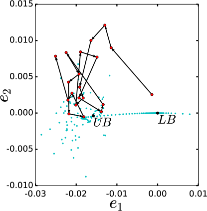
Figure 1: Unstable manifold of LB (cyan dots) and a small perturbation (red circles) to the laminar flow that develops into a puff on the Poincaré section (9). Direction of discrete time from $n=0$ to $n=20$ is indicated by arrows for the perturbation. Intersection of relative periodic orbits LB and UB are marked black and annotated. Few points on the unstable manifold to the right side of LB are shown as this direction consist of laminarizing orbits.

4 The unstable manifold

Budanur & Cvitanović (2015), demonstrate the computation of one- and two-dimensional unstable manifolds of relative periodic orbits on Poincaré sections for the Kuramoto-Sivashinsky system. The main idea is to select trajectories that approximately cover the linear unstable manifold, hence their forward integration approximately covers the nonlinear unstable manifold; see  Budanur & Cvitanović (2015) for details. Here, we are interested in computing the unstable manifold of the lower-branch relative periodic orbit (LB) of  Avila et al. (2013) at $\textit{Re}=1700$. At this Re, the only unstable Floquet multiplier of LB is $\Lambda_{1}=2.8291523$. Initial conditions on the Poincaré section that approximately cover the associated unstable manifold are

$$\hat{a}_{\cal P}(\delta)=\hat{a}_{p,{\cal P}}\pm\epsilon\Lambda^{\delta}_{1}\hat{V}_{1,{\cal P}}\,,\quad$$ (11)

where $\delta\in[0,1)$ and $\epsilon$ is a small constant. We set $\epsilon=10^{-4}$ and discretize $\delta$ by taking $9$ equidistant points in $[0,1)$.

Fig. 1 shows the unstable manifold approximated this way. Here, we show the first $20$ intersections of each trajectory with the Poincaré section, projected onto bases formed by the unstable Floquet vector $\hat{V}_{1}$ and the least stable Floquet vector $\hat{V}_{4}$ of LB, orthonormalized by the Gram-Schmidt procedure, namely $e_{1}=\langle\hat{a}_{\cal P}-\hat{a}_{p},\hat{V}_{1,\bot}\rangle,\,e_{2}=\langle\hat{a}_{\cal P}-\hat{a}_{p},\hat{V}_{4,\bot}\rangle$, where subscript $\bot$ implies that vectors are orthonormalized. We observed that as the trajectories leave the neighbourhood of LB (the origin of fig. 1) they approach the UB. This indicates the existence of a heteroclinic connection between the two. Another trajectory shown on fig. 1 is an initially small perturbation developing into a puff. We generated this perturbation by scaling down a typical puff state and found that it approached the UB before redeveloping into a puff.

In order to confirm apparent approaches to the UB, we measured the trajectories’ distance from it on the Poincaré section. Fig. 2(a) shows the distance of an orbit on the unstable manifold of LB and the perturbation we show on fig. 1 from the UB. For both trajectories, we see a clear initial drop before they move away following the unstable manifold of the UB. Note that some of the intersections of initially small perturbation’s trajectory with the Poincaré section appear closer to the UB than its closest approach ($n=4$) in fig. 1. This is an artefact of low-dimensional projection from an infinite dimensional Poincaré section. For further comparison, we show the time-evolution of turbulent kinetic energy for both trajectories on fig. 2(b). Note for the trajectory on the unstable manifold that before the kinetic energy goes up to puff levels ($\sim 1.4k_{HP}$) it oscillates around $0.5k_{HP}$ during $\tau\in(125,175)(D/U)$. Similarly, for the small perturbation, after initial increase, the kinetic energy stays close to $0.6k_{HP}$ during $\tau\in(25,75)(D/U)$ before further increasing to puff levels. Both episodes corresponds to trajectories’ approach to UB. Note that the time interval shown in fig. 2(a) is not necessarily the same for each orbit, nor are the discrete time intervals equal to each other. For the perturbation, the interval $n\in[0,20]$ to $\tau\in(0,146.25)\,(D/U)$, whereas for the trajectory on the unstable manifold, it corresponds to $\tau\in(0,193.67)\,(D/U)$.

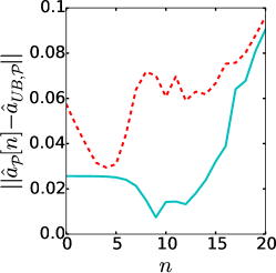
(a)   (b)

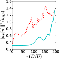
Figure 2: (a) $L_{2}$ Distance from UB on the Poincaré section for $20$ returns, (b) Time-evolution of kinetic energy in units of the kinetic energy $k_{HP}$ of the laminar flow. Cyan (solid): A trajectory on the unstable manifold of LB, red (dashed): puff transition initiated by a small perturbation to the laminar state.

(a)
(b)
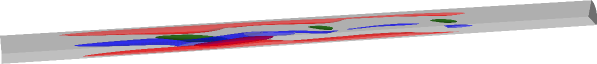
(c)
(d)
(e)
(f)

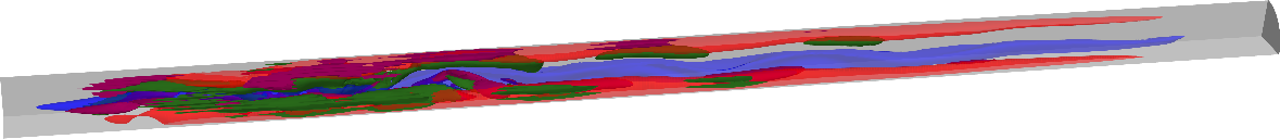
Figure 3: isosurfaces of streamwise vorticity at $\omega_{z}=\pm 0.5U/D$ (pink and green) and streamwise velocity at $u=\pm 0.1U$ (red and blue) for the trajectory on LB’s unstable manifold at $n=0,9,20$ (a, c, f), for the small perturbation at $n=0,4,20$ (b, d) and for UB (e). Shown here is the pipe region $z\in[5,20]D\,,\theta\in[0,\pi/2]$ since rest of the structures can be obtained from reflection and rotation by $\pi$ symmetries that are present.

For further comparison, we visualized streamwise velocity and vorticity isosurfaces of these orbits and the UB on fig. 3. At the closest approach ($n=9$, fig. 3 (c)) the resemblance of flow structures of the unstable manifold with those of UB (fig. 3 (e)) is very close. While not as dramatic, at closest approach ($n=4$, fig. 3 (d)) of the initially (fig. 3 (b)) small perturbation’s to UB, we also see structural resemblance. The same isosurfaces for the LB are visually indistinguishable from the initial point ($n=0$, fig. 3 (a)) on the unstable manifold, hence not separately shown in fig. 3. Note that puffs are structurally (fig. 3 (f)) much more complicated than $LB$ and $UB$.

In order to compare sizes of turbulent structures, we plotted the kinetic energy of fluctuations as a function of axial position, i.e. $k(z)=\frac{1}{2}\int_{0}^{D/2}\int_{0}^{2\pi}{\bf u}\cdot{\bf u}\,rdrd\theta$, for the trajectory on the unstable manifold of LB. Fig. 4 (a) shows the time interval $n\in[0,9]$, during which the orbit leaves the neighbourhood of LB and approaches to UB. During the time-interval $n\in[10,20]$ shown in fig. 4 (b), the orbit moves away from UB and becomes a puff.

5 Conclusion and outlook

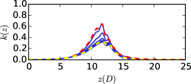
(a) (b)

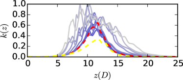
Figure 4: Fluctuating kinetic energy $k(z)$ (arbitrary units) contained at an axial location $(z)$ for $n=0,1,\ldots,9$ and $n=10,11,\ldots,20$ (b). Darkest shade of blue corresponds to initial time $n=0$, and the plotting colour becomes lighter as time increases. Dashed yellow and red curves correspond to the LB and the UB. $k(z)$ values are normalized by their maximum.

In this paper, we presented strong numerical evidence of a heteroclinic connection between two spatially localized relative periodic orbits of pipe flow. This is a remarkable example of structural stability in a dynamical system since these orbits born of a saddle-node bifurcation at $\textit{Re}\approx 1430$ yet their dynamical connection persists at $\textit{Re}=1700$. We repeated our unstable manifold calculation at $\textit{Re}=1900$ and obtained a qualitatively similar picture.

Previous studies  (Halcrow et al., 2009; van Veen & Kawahara, 2011) reported homoclinic and heteroclinic connections in Couette flow, which can accommodate equilibria and periodic orbits without spatial drifts. This is not the case for pressure-driven flows since all invariant solutions except the laminar equilibrium have non-zero streamwise drifts. In this regard, the current work fills an important technical gap and provides a new set of tools for study of pressure-driven flows. While, the methods we used here appeared in different publications (Budanur et al., 2015; Ding et al., 2016; Budanur & Cvitanović, 2015), where they are applied to much lower-dimensional systems, this is their first application to the full Navier-Stokes equations.

While  Avila et al. (2013) shows that the chaotic motion emerges from the bifurcations of the UB, as the Reynolds number is increased from $1430$ to $1545$, the role of UB for transition is not obvious at $\textit{Re}=1700$. Our result shows that far from the bifurcation point, the UB takes the role of mediating the transition. To the best of our knowledge, this is the first example of an upper-branch solution in a shear flow that lies between laminar and the turbulent parts of the state space, similar to lower-branch. Note that UB, whose kinetic energy swings around $k=0.5k_{HP}$, is energetically separated from turbulent puffs which have typical kinetic energies $k\approx 1.2k_{HP}$. This is also clearly visible from the axial distribution of kinetic energies on fig. 4 and flow structures on fig. 3, where the UB clearly has a much simpler structure than puffs.

The time evolution of the spatial distribution of the kinetic energy on fig. 4 suggests a two-stage transition scenario, where the spatial complexity of a puff forms as trajectories follow the unstable manifold of UB (fig. 4 (b)).  Ritter et al. (2016) recently reported a detailed numerical study, where they used turbulent kinetic energy and pressure gradient as indicators to support the hypothesis that spatial complexity in this system arises as different chaotic regions in the state space merge with the neighbourhood of the UB. These observations along with ours motivate a detailed study of UB’s unstable manifold in order to understand spatial expansion of chaotic spots. The tools we introduce here can be useful for such a study.

Appendix A Projection operator

Figure 5: Schematic illustration of the transformation of $a$ and a small perturbation $\delta a$ to it by the nonlinear group action ${f^{\phi}(a)}$ onto the hypersurface $U(\hat{a})=0$.

The projection operations (8) and (10) follow from the same geometrical principle, which we are going to derive here. Let ${f^{\phi}(a)}$ be the nonlinear semi-group action that transforms the state-space vector $a$ according to the parameter $\phi$ as

$$a^{\prime}={f^{{\phi}}(a)}\,,\quad{\phi}\in[0,{\phi}_{max})$$ (12)

and let $U(a)$ be a scalar-valued function of $a$ that defines a codimension-1 hypersurface $U(\hat{a})=0$ in the state-space such that at $\hat{a}={f^{{\hat{\phi}}}(a)}$ a semi-group orbit of $a$ intersects this hypersurface transversally as illustrated in fig. 5. Now let us consider a small perturbation $\delta a$ to $a$ and its transformation onto this hypersurface:

$$\hat{a}+\delta\hat{a}={f^{{\hat{\phi}}+\delta{\hat{\phi}}}(a+\delta a)}\,.$$ (13)

Taylor expanding the RHS to linear order in $\delta{\hat{\phi}}$ and $\delta a$ we obtain

$$\delta\hat{a}=\partial_{\phi}{f^{{\phi}}(a)}|_{{\phi}={\hat{\phi}}}\delta{\hat{\phi}}+\left.\frac{d{f^{{\phi}}(a^{\prime})}}{da^{\prime}}\right|_{a^{\prime}=a}\delta a\,.$$ (14)

Our goal is to find an expression for $\delta\hat{a}$, however, (14) gives us one condition with two unknowns $\delta\hat{a}$ and $\delta{\hat{\phi}}$. The second condition comes from the fact that (13) also satisfies the hypersurface equation, i.e. $U(\hat{a}+\delta\hat{a})=0$. Taylor expansion to the linear order yields

$$\left\langle\left.\frac{dU(a)}{da}\right|_{a=\hat{a}},\,\delta\hat{a}\right\rangle = 0\,,$$

$$\left\langle\left.\frac{dU(a)}{da}\right|_{a=\hat{a}},\,\partial_{\phi}{f^{{\phi}}(a)}|_{{\phi}={\hat{\phi}}}\right\rangle\delta{\hat{\phi}}+\left\langle\left.\frac{dU(a)}{da}\right|_{a=\hat{a}},\,\left.\frac{d{f^{{\phi}}(a^{\prime})}}{da^{\prime}}\right|_{a^{\prime}=a}\delta a\right\rangle = 0\,,$$ (15)

where in the second step we inserted (14) for $\delta\hat{a}$. Solving (15) for $\delta{\hat{\phi}}$ and inserting its expression into (14) we find

$$\delta\hat{a}=\left.\frac{d{f^{{\phi}}(a^{\prime})}}{da^{\prime}}\right|_{a^{\prime}=a}\delta a-\partial_{\phi}{f^{{\phi}}(a)}|_{{\phi}={\hat{\phi}}}\frac{\left\langle\left.\frac{dU(a)}{da}\right|_{a=\hat{a}},\,\left.\frac{d{f^{{\phi}}(a^{\prime})}}{da^{\prime}}\right|_{a^{\prime}=a}\delta a\right\rangle}{\left\langle\left.\frac{dU(a)}{da}\right|_{a=\hat{a}},\,\partial_{\phi}{f^{{\phi}}(a)}|_{{\phi}={\hat{\phi}}}\right\rangle}\,,$$ (16)

which we can rewrite as

$$\delta\hat{a}=\left(\textbf{1}-\frac{\partial_{\phi}{f^{{\phi}}(a)}|_{{\phi}={\hat{\phi}}}\otimes\left.\frac{dU(a)}{da}\right|_{a=\hat{a}}}{\left\langle\left.\frac{dU(a)}{da}\right|_{a=\hat{a}},\,\partial_{\phi}{f^{{\phi}}(a)}|_{{\phi}={\hat{\phi}}}\right\rangle}\right)\left.\frac{d{f^{{\phi}}(a^{\prime})}}{da^{\prime}}\right|_{a^{\prime}=a}\delta a\,,$$ (17)

where $\otimes$ denotes the outer product. Both projection operators (8) and (10) can be obtained from (17) by substitutions $(l,g(l)a)\rightarrow({\phi},{f^{{\phi}}(a)})$ and $(\tau,{f^{\tau}(a)})\rightarrow({\phi},{f^{{\phi}}(a)})$ respectively.

References

- Avila et al. (2011) Avila, K., Moxey, D., de Lozar, A., Avila, M., Barkley, D. & Hof, B. 2011 The onset of turbulence in pipe flow. Science 333, 192–196.
- Avila et al. (2013) Avila, M., Mellibovsky, F., Roland, N. & Hof, B. 2013 Streamwise-localized solutions at the onset of turbulence in pipe flow. Phys. Rev. Lett. 110, 224502.