White dwarf dynamical interactions and fast optical transients

Abstract

Recent advances in time-domain astronomy have uncovered a new class of optical transients with timescales shorter than typical supernovae and a wide range of peak luminosities. Several subtypes have been identified within this broad class, including Ca-rich transients, .Ia supernovae, and fast/bright transients. We examine the predictions from a state-of-the-art grid of three-dimensional simulations of dynamical white dwarf interactions in the context of these fast optical transients. We find that for collisions involving carbon-oxygen or oxygen-neon white dwarfs the peak luminosities and durations of the light curves in our models are in good agreement with the properties of fast/bright transients. When one of the colliding white dwarfs is made of helium the properties of the light curves are similar to those of Ca-rich gap transients. The model lightcurves from our white dwarf collisions are too slow to reproduce those of .Ia SNe, and too fast to match any normal or peculiar Type Ia supernova.

1 Introduction

The advent of photometric surveys combining wide field capabilities with a fast cadence of visits, like PTF (Law et al., 2009) and Pan-STARRS (Kaiser et al., 2002), has led to significant advances in time-domain astrophysics. In particular, these surveys have uncovered a new class of astronomical transients with timescales faster than the $\sim$20 days typical of Type Ia supernovae (SNe Ia), and a wide range of peak luminosities, which we will broadly categorize as ‘fast transients’. Because this is an emerging field, the full observational range of fast transients has yet to be characterized, but several sub-classes have already been described in the literature — see the left panel of Figure 1, adapted from Kasliwal (2012). The so-called ‘fast and bright’ transients (Perets et al., 2011) were identified partly through historical observations of SN 1885 and SN 1939B. They are as luminous as normal SNe Ia  ($L\sim 10^{43}$ erg s^-1, or $M_{V}\sim-18$), but have timescales of $\sim 10$ days, faster than even the faintest, more rapidly evolving SNe Ia. The somewhat awkwardly named .Ia SNe (Bildsten et al., 2007; Poznanski et al., 2010; Kasliwal et al., 2010) have luminosities similar to fast/bright transients, but even faster timescales of only a few days. Ca-rich gap transients have timescales similar to fast/bright transients, but are an order of magnitude fainter at peak ($L\sim 10^{42}$ erg s^-1, or $M_{V}\sim-16$), and show strong nebular features from Ca in their late-time spectra (Filippenko et al., 2003; Perets et al., 2010; Kasliwal et al., 2012). Finally, there are some fast transients like SN2008ha that do not seem to fit into any of these categories (Foley et al., 2010). At present, it is still unclear to what degree these classes are physically distinct or internally homogeneous, and it is likely that the taxonomy of fast transients will evolve in the near future.

Our understanding of the stellar progenitors for each subclass of these fast transients is still very limited. The exception are .Ia SNe, which were theoretically predicted by Bildsten et al. (2007) to arise from the thermonuclear detonation of a helium shell on an accreting white dwarf. Their observational counterparts were later identified by Kasliwal et al. (2010), and found to exhibit many features in agreement with this model, so this subclass has at least a viable progenitor scenario — but see Shen et al. (2010) for a discussion. The situation is less clear for the other two subclasses. Perets et al. (2011) proposed a white dwarf origin for fast/bright transients, based on the old stellar environments around SN 1885 and SN 1939B, the low ejecta masses inferred from the short timescales, and the lack of detectable X-ray emission after more than 130 years from SN 1885.

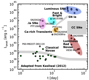
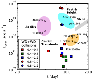
Figure 1: Left panel: peak luminosity as a function of the characteristic timescale for several optical transients, with some relevant subclasses highlighted in color — adapted from Kasliwal (2012). Right panel: location of several simulations of colliding white dwarfs, for different initial conditions, masses and chemical compositions of the interacting white dwarfs, overlayed on the observational subclasses discussed in the text.

A number of competing models are being considered for Ca-rich transients, including gravitational core collapse of stripped massive stars (Kawabata et al., 2010), the coalescence of a binary system made of a neutron star and a white dwarf (Metzger, 2012; Sell et al., 2015), and the merger of two white dwarfs, one of them with a carbon-oxygen (or an oxygen-neon) core and the second one made of helium (Perets et al., 2010; Kasliwal et al., 2012). The first of these scenarios, namely the explosion of a rather massive star ($M\ga 8\,M_{\sun}$), seems to be in contradiction with the prevalence of early-type host galaxies for these outbursts, and with the fact that Ca-rich transients occur predominantly in galaxies with no apparent signs of recent star formation (Perets et al., 2010; Lyman et al., 2013). Moreover, Ca-rich transients occur predominantly in the outskirsts of galaxies (Kasliwal et al., 2012; Lyman et al., 2014; Foley, 2015), and their locations do not trace the stellar light of their host galaxies, at odds with what occurs with other luminous transients and supernovae (Anderson et al., 2015). This led to the suggestion that these events are due to explosions in old white dwarfs belonging to faint globular clusters or dwarf galaxies, which are difficult to detect — see, for instance, Waldman et al. (2011). However, Lyman et al. (2014) obtained deep VLT images of two members of the class (SN 2005E and 2012hn) and found no evidence for any underlying stellar population. More recently, Lyman et al. (2016) analyzed HST data of five objects of the class (SN 2001co, SN 2003dg, SN 2003dr, SN 2005E, and SN 2007ke) and corroborated their previous findings. This failure to identify faint and dense stellar systems — like globular clusters, or dwarf galaxies — as the underlying population does not necessarily mean that these transients could not have been originated in other old stellar populations — like stellar haloes — which would be too faint to be detected, even with image stacking — see Perets (2014), and references therein. Nevertheless, a cautionary remark is in order here, as the rate at which these collisions occur in typical old stellar populations is expected to be small (Perets, 2014). In summary, the issue of the origin of Ca-rich transients remains unresolved.

An interesting possibility is that the progenitors of Ca-rich transients are not formed at large offsets from their parent galaxies, but instead that they have travelled large distances because of their large peculiar velocities (Lyman et al., 2014). This, in turn, could point towards a dynamical interaction of a white dwarf with another compact object, either a black hole (Sell et al., 2015; MacLeod et al., 2016), a neutron star (Metzger, 2012), or a white dwarf (Brown et al., 2011; Foley, 2015), in which the system acquires a sufficiently high kick. Since dynamical interactions (either mergers or collisions) between two white dwarfs should be more common than those between a black hole or a neutron star and a white dwarf, the former channel should be more likely. Indeed, we know from the distribution of radial velocities in multi-epoch observations of Galactic white dwarfs that coalescences and/or collisions happen at a rate comparable to SNe Ia  (Badenes & Maoz, 2012; Maoz & Hallakoun, 2016), which imples that their observational counterparts, whatever they may be, must be relatively common. In this scenario, the explosion could be the result of the merger of double white dwarf binary system where the components are brought together by gravitational wave radiation, or it could be triggered by a stellar close encounter, perhaps prompted by Kozai oscillations in a triple system (Thompson, 2011; Katz & Dong, 2012; Antognini et al., 2014) — see Sect. 2. In either case, the expectation is that for some interactions an explosion will occur at the base of the accreted buffer that is formed after the disruption of the less massive star.

Here we study the possibility that some of these fast transients arise from dynamical interactions between two white dwarfs that are triggered either by random encounters in dense stellar environments or by the coalescence of binary pairs. Although the physical mechanisms driving white dwarf mergers and collisions are quite different, the overall properties of the dynamical interaction are similar for similar masses of the interacting white dwarfs. More importantly, in both cases variable amounts of nickel are synthesized in the ensuing thermonuclear flash, thus powering quite different light curves. This could help to explain the observed features of some transients. Perhaps the single major, but significant, difference of between white dwarf mergers and collisions is that in white dwarf mergers the debris region surrounding the central compact object consists of a Keplerian disk, while in white dwarf collisions the disk, if present, is embedded in a shroud of high-velocity material. Finally, it is also worth mentioning that in some white dwarf collisions the velocity field of the remnant of the interaction is highly asymmetric. Thus, owing to linear momentum conservation, the remnants of the interaction can move at considerable speeds. This may explain why the distribution of the locations of Ca-rich transients is strongly skewed to very large galactocentric offsets Anderson et al. (2015), unlike other luminous transients and SNe.

In this paper, we explore the predictions from a model grid of white dwarf dynamical interactions (Aznar-Siguán et al., 2013) in the context of the newly identified subclasses of fast transients. We have chosen this model grid because it is the most consistent suite of calculations, although the results of other sets of calculations of merging or colliding white dwarfs are quantitatively similar. Our work is organized as follows. In Sect. 2 we review the different sets of calculations of white dwarf dynamical interactions. In Sect. 3 we discuss the light curves resulting from our dynamical white dwarf interaction models. We show that when one of the colliding white dwarfs is made of carbon and oxygen, the peak luminosities and timescales agree with those of fast/bright transients, and when one of the white dwarfs has a helium core, they are similar to those of Ca-rich transients. In Sect. 4 we argue that the calcium yields in our models, and their spatial distribution, are also in reasonable agreement with the observations of some Ca-rich transients. Finally, in Sect. 5 we summarize our findings and we describe our conclusions.

2 White dwarf dynamical interactions

White dwarf dynamical interactions can be classified in two main categories: white dwarf mergers, and white dwarf collisions. White dwarf mergers are driven by the emission of gravitational waves, whereas white dwarf collisions occur when two white dwarfs pass close to each other, and gravitational focusing brings them so close that the less gravitationally bound star transfers mass to the massive member of the system. In both cases the result is that the lighter white dwarf is destroyed during the interaction and its material is accreted onto the heavier white dwarf.

In white dwarf mergers the accretion episode occurs when the secondary star overflows its Roche lobe, while in white dwarf collisions the secondary usually begins transferring mass at periastron. Once the dynamical interaction between the two white dwarfs begins, the process of disruption of the lightest member of the system is accelerated, due to the inverse dependence of the radius of white dwarfs on the mass. Depending on the masses of the coalescing white dwarfs and on the corresponding mass ratio the process can be very fast, and a common result is that the disruption takes place in a few orbital periods for the case of white dwarf mergers, and on short timescales for white dwarf collisions in which the low-mass member of the pair is captured in a highly eccentric orbit, typically in a few orbits as well. In both cases it turns out that the material transferred to the heavier star is compressed and heated to such an extent that, in some cases, the conditions for a detonation are met. This, of course, depends on the initial conditions of the dynamical interaction, and on the masses and chemical compositions of the intervening white dwarfs.

White dwarf mergers have been extensively studied during the last few years, because they may possibly account for a sizable fraction of normal Type Ia supernova explosions. The pioneering Smoothed Particle Hydrodynamics (SPH) calculations of Benz et al. (1989a, b); Benz et al. (1990) paved the way to what now is a mature research field. These early calculations were followed some time later by more accurate studies (Rasio & Shapiro, 1995; Segretain et al., 1997). However, progress was slow in subsequent years, until new sets of numerical calculations overcoming some of the limitations of the previous simulations became available (Guerrero et al., 2004; Yoon et al., 2007). In these new calculations enhanced spatial resolutions, improved prescriptions for the artificial viscosity, updated nuclear reaction rates, and realistic equations of state were employed to cover a wider range of masses and chemical compositions of the merging white dwarfs. The most recent sets of numerical calculations of merging white dwarfs (Lorén-Aguilar et al., 2009; Pakmor et al., 2010, 2011; Dan et al., 2011; Pakmor et al., 2012b, a; Dan et al., 2012; Raskin et al., 2012; Pakmor et al., 2013; Kromer et al., 2013; Zhu et al., 2013; Dan et al., 2014; Moll et al., 2014; Raskin et al., 2014; Zhu et al., 2015; Marquardt et al., 2015; Tanikawa et al., 2015; Sato et al., 2015; Dan et al., 2015) have come to an agreement about the evolution during the merger episode and the characteristics of the merged remnant. In particular, there is a general consensus that little mass is ejected from the system during the interaction, and that a violent merger (that is, a merger in which a prompt explosion takes place) does not occur except in those cases in which two rather massive ($\sim 0.9\,M_{\sun}$) carbon-oxygen white dwarfs of similar masses merge. Moreover, in those mergers that do not experience a powerful detonation, and consequently are not totally disrupted, about half of the mass of the secondary is accreted onto the primary star of the pair, while the rest of the mass forms a debris region which for unequal mass mergers is a Keplerian rotating disk. Additionally, variable amounts of nickel and intermediate-mass elements are synthesized and, consequently, the peak luminosities of the corresponding light curves span a considerable range — see Fig. 1. The resulting nucleosynthesis is sensitive to the mass ratio and to the chemical composition of the coalescing white dwarfs.

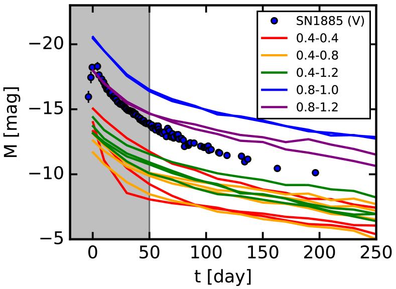
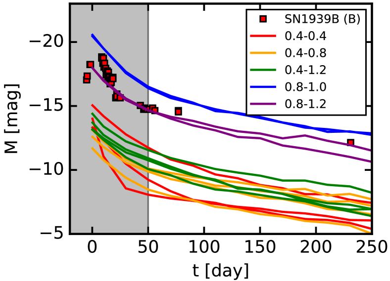
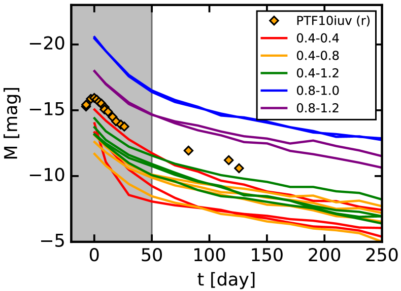
Figure 2: Light curves of SN 1885, SN 1939B, and PTF 10iuv — from Perets et al. (2011) and Kasliwal et al. (2012) — compared to the predicted light curves from our models. The regime below 50 days after peak, where our calculated light curves are more approximative, is shaded in gray. The lightcurve of PTF10iuv has been corrected for host galaxy contamination as described in Kasliwal et al. (2012).

The study of white dwarf collisions was also pioneered by Benz et al. (1989c), who employed a SPH code to simulate the collisions of two systems of white dwarfs of masses $0.6\,M_{\sun}$ and $0.6\,M_{\sun}$, and $0.9\,M_{\sun}$ and $0.7\,M_{\sun}$, respectively. For two decades this study remained the only one to examine white dwarf collisions. The first recent study of white dwarf collisions was performed by Rosswog et al. (2009). However, Rosswog et al. (2009) limited their study to head-on collisions, although they investigated the characteristics of the dynamical interaction for several masses of the colliding carbon-oxygen white dwarfs. Almost simultaneously, Raskin et al. (2009) examined the collision of two otherwise typical white dwarfs of equal masses ($0.6\,M_{\sun}$) for different impact parameters and mass resolutions. In the same vein, Lorén-Aguilar et al. (2010) explored the collisions of one mass pair (of unequal masses, $0.6\,M_{\sun}$ and $0.8\,M_{\sun}$) for various impact parameters. Later on, Raskin et al. (2010) expanded their previous study to encompass pairs of different masses and collisions with different impact parameters. In all these sets of simulations state-of-the-art SPH codes were employed. Moreover, reliable equations of state, and large numbers of SPH particles (ranging from $4\times 10^{5}$ to $2\times 10^{6}$) were adopted. Finally, García-Senz et al. (2013) studied the head-on collision of two twin white dwarfs of mass $0.7\,M_{\sun}$, but although they used a very high mass resolution, the simulations were not three-dimensional. The only studies in which a SPH code was not employed are those of Hawley et al. (2012), Kushnir et al. (2013a) and Papish & Perets (2016). In all cases the Eulerian adaptive grid code FLASH was used. Hawley et al. (2012) studied two twin pairs of masses $0.64\,M_{\sun}$, and $0.81\,M_{\sun}$, whereas Papish & Perets (2016) considered several masses of the colliding white dwarfs, from $0.6\,M_{\sun}$ to $0.8\,M_{\sun}$, and Kushnir et al. (2013a) performed two-dimensional hydrodynamical simulatiosn of zero-impact-parameter collisions of white dwarfs with masses between $0.5$ and $1.0\,M_{\sun}$. It is noteworthy that in all these simulations the colliding white dwarfs were made of carbon and oxygen.

Table 1: Calcium masses (in solar masses) for the white dwarf collisions of Aznar–Siguán et al. (2013) that result in an explosion.

$M_{1}+M_{2}$	$v_{\rm ini}$	$\Delta y$	$M_{\rm Ca}$	$M_{\rm Ni}$	$M_{\rm Fe}$
$(M_{\sun})$	(km s-1)	$(R_{\sun})$	$(M_{\sun})$	$(M_{\sun})$	$(M_{\sun})$
0.4+1.2	150	0.3	$7.3\times 10^{-3}$	$8.4\times 10^{-4}$	$1.6\times 10^{-2}$
0.4+1.2	100	0.3	$7.0\times 10^{-3}$	$2.2\times 10^{-3}$	$2.0\times 10^{-2}$
0.4+1.2	100	0.4	$7.3\times 10^{-3}$	$9.4\times 10^{-4}$	$1.3\times 10^{-2}$
0.4+1.2	75	0.4	$7.4\times 10^{-3}$	$1.2\times 10^{-3}$	$1.5\times 10^{-2}$
0.4+0.8	150	0.3	$8.5\times 10^{-3}$	$2.0\times 10^{-4}$	$5.4\times 10^{-3}$
0.4+0.8	100	0.3	$8.4\times 10^{-3}$	$7.6\times 10^{-4}$	$1.7\times 10^{-2}$
0.4+0.8	100	0.4	$8.5\times 10^{-3}$	$5.0\times 10^{-4}$	$9.0\times 10^{-3}$
0.4+0.8	75	0.4	$8.2\times 10^{-3}$	$8.0\times 10^{-4}$	$1.2\times 10^{-2}$
0.4+0.4	100	0.3	$1.9\times 10^{-2}$	$4.7\times 10^{-3}$	$2.9\times 10^{-2}$
0.4+0.4	75	0.3	$1.8\times 10^{-3}$	$8.8\times 10^{-4}$	$1.7\times 10^{-2}$
0.4+0.4	75	0.4	$2.0\times 10^{-2}$	$1.6\times 10^{-3}$	$1.9\times 10^{-2}$
0.4+0.2	75	0.3	$1.6\times 10^{-3}$	$1.3\times 10^{-9}$	$3.5\times 10^{-7}$
0.8+1.2	100	0.3	$1.9\times 10^{-2}$	$6.3\times 10^{-2}$	$3.6\times 10^{-3}$
0.8+1.2	75	0.4	$1.9\times 10^{-2}$	$6.3\times 10^{-2}$	$3.6\times 10^{-3}$
0.8+1.0	100	0.3	$6.3\times 10^{-2}$	$7.2\times 10^{-1}$	$1.6\times 10^{-2}$
0.8+1.0	75	0.4	$6.5\times 10^{-2}$	$7.3\times 10^{-1}$	$1.6\times 10^{-2}$

Inspired in part by the observational discoveries previously mentioned in Sect. 1, and by the recent theoretical efforts discussed in the previous paragraphs, Aznar-Siguán et al. (2013) computed a grid of white dwarf collisions, considering a large interval of initial conditions and a broad range of masses and core chemical compositions of the interacting white dwarfs. This suite of simulations, together with that of Raskin et al. (2010) are the most comprehensive sets of calculations of white dwarf collisions performed so far, and supplement previous calculations of this kind. However, the advantage of the simulations of Aznar-Siguán et al. (2013) over the rest of theoretical calculations is that they explored the role of the core composition of the colliding white dwarfs. In particular, they computed in an homogenous way a suite of collisions in which one of the components of the pair of white dwarfs was made of helium, carbon-oxygen, or oxygen-neon, whereas the second member of the system was made of helium or carbon-oxygen. This particular feature of the simulations of Aznar-Siguán et al. (2013) is important, because it opens new and interesting possibilities for observational counterparts, that need to be explored. As a matter of fact, the calculations of Aznar-Siguán et al. (2013) reveal that, independently of the core compositions of the interacting white dwarfs, the result of the dynamical interaction has several remarkable characteristics. The first of them is that the remnant of the interaction is surrounded by a shroud of material moving at considerable speeds. The second is that variable amounts of intermediate-mass elements are synthesized, depending on the chemical composition of the colliding white dwarfs. The amount of radioactive nickel resulting in these simulations spans a considerable range, resulting in very different peak luminosities of the corresponding light curves. Finally, because of the large asymmetry of the velocity field resulting from the dynamical interaction, the debris region can move at sizable speeds, imparting an asymmetric kick to the ejecta. In summary, all these characteristics of the theoretical calculations deserve further attention, and consequently it is worth studying the possibility that they could explain, at least partially, some of the observed properties of fast optical transients.

3 Peak luminosities, decay times, and light curves

Aznar-Siguán et al. (2013) showed that in some cases the outcome of white dwarf close encounters could be a direct collision in which only one catastrophic episode of mass transfer between the less-massive star and the massive white dwarf occurs, or lateral collisions characterized by several more gentle mass-transfer episodes. Moreover, they also demonstrated that in a significant number of the cases, the material of the disrupted star is compressed and heated to such an extent that the conditions for detonation are met, reaching peak temperatures of the order of $10^{9}$ K, and even larger for direct collisons, for which temperatures larger than $10^{10}$ K are easily reached. Accordingly, the masses of ⁵⁶Ni synthesized during the detonation span several orders of magnitude, from $\sim 1.3\times 10^{-9}\,M_{\sun}$ to about $0.7\,M_{\sun}$.

Aznar-Siguán et al. (2014) computed the light curves for the simulations in Aznar-Siguán et al. (2013). The peak luminosities of these interactions span a wide range, between $1.5\times 10^{43}$ erg s^-1, which is brighter than even the brightest SN Ia, and $2.7\times 10^{34}$, which is fainter than even typical novae. Obviously, this wide range of peak luminosities is the result of the very different ⁵⁶Ni masses produced during the most violent phases of the interactions. Although Aznar-Siguán et al. (2014) employed an approximate method to compute the light curves, their corresponding durations can be determined with a reasonable degree of accuracy. Specifically, Aznar-Siguán et al. (2014) employed the approximate method of Kushnir et al. (2013b), which provies a relation between the synthesized mass of ⁵⁶Ni and the late-time bolometric light curve. Within this treatment, the late-time light curve is computed numerically using a Monte Carlo algorithm, which solves the transport of photons, and the injection of energy by the $\gamma$ rays produced by the decays of ⁵⁶Ni and ⁵⁶Co. In order to compare with the observed duration of fast optical transients we compute the characteristic timescales of the light curves of Aznar-Siguán et al. (2014) as their width at half the peak luminosity. The time origin is chosen as the point at which the dynamical interaction reaches the peak temperature, which occurs shortly before the peak luminosity is reached. This is close enough to the observational definition of the decay time — the time to decay one magnitude from peak, or a factor of 2.5 in flux (Kasliwal, 2012) — to allow for an approximate comparison between models and observations.

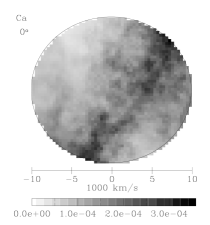
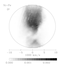
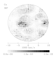
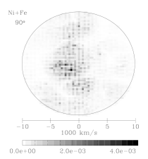
Figure 3: Spatial distribution of the Ca (left panels) and Ni+Fe (right panels) mass abundances for the $0.4+0.4\,M_{\sun}$ merger with $v_{\rm ini}=100$ km s^-1 and $\Delta y=0.4\,R_{\sun}$, and two inclinations, $0^{\circ}$ (top panels) and $90^{\circ}$ (bottom panels), as a function of the average expansion velocity.

In Fig. 1 the results of these numerical calculations are compared to the observational properties of the several subclasses of fast optical transients. In particular, the three main subclasses of fast transients are highlighted in magenta (.Ia SNe), blue (fast/bright transients) and orange (Ca-rich transients). The white dwarfs in our model grid are composed of helium (0.4 $M_{\sun}$), carbon-oxygen (0.8 and 1.0 $M_{\sun}$) and oxygen-neon (1.2 $M_{\sun}$), and the differences between models with identical components are driven mainly by the initial velocities and impact parameters — see Aznar-Siguán et al. (2013) for details. As can be seen in this figure, most of our model light curves have timescales of $\sim 10$ days, clearly faster than those of normal SN Ia and slower than those of .Ia SNe, but comparable to both fast/bright and Ca-rich transients. When both white dwarfs are relatively massive, the transients can be quite bright, with peak luminosities of $\sim 10^{44}$ erg s^-1 for two carbon-oxygen cores, and $\sim 10^{43}$ erg s^-1 for an interaction involving carbon-oxygen and oxygen-neon white dwarfs. These values are comparable with those observed in the fast/bright transients like SN 1885 and SN 1939B. In contrast, dynamical interactions that involve at least one helium white dwarf produce fainter transients with $10^{40}\la L\la 10^{42}$ erg s^-1. The upper end of this range is comparable with the values measured for prototypical Ca-rich transients like SN 2005E. Finally, some models have lower peak luminosities, comparable to those of SN 2008ha, while other models have peak luminosities one order of magnitude lower than this. At present it is unclear whether these interactions have observational counterparts.

A more detailed comparison between our theoretical light curves and the observations of two fast and bright transients — SN 1885 and SN 1939B (Perets et al., 2011) — and a Ca-rich transient — PTF 10iuv (Kasliwal et al., 2012) — is shown in Fig. 2. These comparisons are necessarily qualitative since, as discussed before, our theoretical light curves are only approximate for times below 50 days. However, here we highlight the behavior at late times, up to 250 days, where our calculations are more reliable. In principle, the luminosities in our light curves should not be directly compared to broadband photometric observations without some sort of bolometric correction. This is less of a concern for SN 1885 and SN 1939B, since transients powered by ⁵⁶Ni decay, like all normal and peculiar SN Ia, and our white dwarf interaction models, tend to peak in the $B$ and $V$ band (Ashall et al., 2016), where the historical observations were taken. There might be a larger correction for PTF 10iuv, since the light curve from Kasliwal et al. (2012) is in the $r$ band, but we include the comparison for illustrative purposes because this is the most extended light curve available for a Ca-rich transient. Within these limitations, the comparisons in Fig. 2 show that the lightcurves for models involving carbon-oxygen and oxygen-neon white dwarfs do span the range of peak luminosities and late-time evolution for fast and bright transients. The match between SN 1939B and the carbon-oxygen and oxygen-neon models is particularly good, while the late time decay of SN 1885 seems faster than the models, though not by much. The late time evolution of the Ca-rich transient PTF 10iuv is similar to that of the models which most closely match its peak luminosity, which include the interactions of two white dwarfs made of helium and an oxygen-neon white dwarf with a white dwarf with a helium core.

4 Calcium yields and spatial distribution

Table 1 lists the Ca, Ni, and Fe yields for the runs of Aznar-Siguán et al. (2013) that have an explosive outcome — see Table 6 of Aznar-Siguán et al. (2013). In this table we also show the initial relative velocity ($v_{\rm ini}$) and separation ($\Delta y$) of the interacting white dwarfs. Our dynamical white dwarf interaction models synthesize between $\sim 0.001$ and $\sim 0.06$ $M_{\sun}$ of Ca, with the highest yields corresponding to the 0.8+1.0 $M_{\sun}$  simulation. For the interactions involving at least one helium white dwarf, which provide the best match for the properties of Ca-rich transients, the Ca yield can be as high as $\sim 0.02$ $M_{\sun}$. This is comparable to the 0.03 $M_{\sun}$  of Ca in the model by Waldman et al. (2011) that Dessart & Hillier (2015) matched to the properties of Ca-rich transients.

The spatial distribution of Ca and Fe+Ni is shown in Fig. 3 for a representative model. Namely, a $0.4+0.4\,M_{\sun}$ collision, with initial separation $\Delta y=0.3\,R_{\sun}$ and initial velocity $v_{\rm ini}=75$ km s^-1. These two-dimensional distribution plots, shown for two different planes in the model ejecta, can be directly compared to the HST narrow-band absorption maps of SN 1885 — Fig. 8 in Fesen et al. (2015). There are remarkable qualitative similarities between these observed maps and the model results. The distribution of the elements in velocity space is similarly compact, and shows a large degree of assimmetry. In particular, little material has velocities in excess of 10,000 km s^-1. Moreover, our sample model also shows very clumpy and asymmetric ejecta, just like the SN 1885 images. Specifically, in the Ca map the $0^{\circ}$ projection shows a prominent band extending from $\sim-5,000$ to $\sim 7,000$ km s^-1, whereas the Fe+Ni distribution shows two prominent clumps at low velocities, being the top one more evident. All these features have roughly the same angular size as the ones seen in the SN 1885 map. In the Fe+Ni map, the $90^{\circ}$ projection shows some filamentary structure that is reminiscent of, albeit less marked than, the one seen in SN 1885. However, we emphasize that the detailed structure of the debris region depends sensitively on the orientation with respect to the line of sight, and that for some inclinations the filamentary structure is more evident. Almost the same can be said for the Ca map at $90^{\circ}$, for which two clear structures can be seen at opposite directions, having velocities of $\sim-4,000$ km s^-1, and $\sim 7,000$ km s^-1, respectively. Note that Fesen et al. (2015) argued that SN 1885 was a sub-luminous Type Ia supernova with an ejected mass close to the Chandrasekhar limit. However, Perets et al. (2011) based on the lack of X-ray emission 130 yr after the explosion, and on the shape of the light curve, did not find clear evidence for this. A more detailed comparison between model lightcurves and the historical data for SN 1885, as well as a statistical analysis of the HST images in the context of multi-dimensional explosion models will settle this issue. We defer these comparisons to future work.

The total mass of Ca for SN 2005E is $0.135\,M_{\sun}$ (Perets et al., 2010), and substantially smaller, $0.054\,M_{\sun}$, for PTF 10iuv (Kasliwal et al., 2012). The Ca masses obtained in our simulations — see Table 1 — are somewhat smaller, albeit comparable to those of Ca-rich transients. For instance, for the simulation presented in Fig. 3, which shows the spatial distribution of Ca for the collision of two helium white dwarfs, the total Ca mass is $\sim 0.02\,M_{\sun}$. Nevertheless, a cautionary note is in order here, since the observed Ca masses are somewhat uncertain, as they are sensitive to the adopted temperature of the nebular spectrum. In fact, a change of the nebular temperature can result in a sizable change in the derived masses (Kasliwal et al., 2012).

5 Summary and conclusions

We have explored the fundamental properties (light curve timescales, peak luminosities, and nucleosynthetic yields) of a grid of white dwarf collision models by Aznar-Siguán et al. (2013), and we have compared them to the known properties of fast transients. These collisions are not frequent, except in dense stellar environments, and their observational counterparts have not been clearly identified yet. We find that collisions in which at least one of the interacting stars is a helium white dwarf match the properties of Ca-rich transients like SN 2005E and unclassified transients like SN 2008ha, while collisions that have more massive components (carbon-oxygen or oxygen-neon white dwarfs) match those of fast/bright transients, like SN 1885 or SN 1939B. In particular, we find that the timescales of the light curves of those collisions in which one of the members of the system is a white dwarf with a helium core are compatible with Ca-rich transients. Also, the mass of Ca in the debris region formed around the more massive white dwarf, which remains almost intact during the dynamical interaction, is comparable to that measured in these transients. The velocities of the material in this region are also consistent with the measured velocities of the ejecta of Ca-rich transients. Moreover, the spatial distribution of Ca-, Ni- and Fe-rich material resembles the observed distributions around Ca-rich transients. Finally, it is worth mentioning that all of our models produce light curves that are faster than those of SNe Ia, but slower than those of .Ia SNe. Nevertheless, we emphasize that more studies are needed to confirm or rule out whether these interactions are indeed the progenitors of at least a fraction of fast optical transients. Looking to the future, further work should focus on detailed radiative transfer modeling of light curves and spectra to compare with extant and future observations. This would allow a better comparison with observations.

References

- Anderson et al. (2015) Anderson J. P., James P. A., Habergham S. M., Galbany L., Kuncarayakti H., 2015, Publ. Astron. Soc. Australia, 32, e019
- Antognini et al. (2014) Antognini J. M., Shappee B. J., Thompson T. A., Amaro-Seoane P., 2014, MNRAS, 439, 1079
- Ashall et al. (2016) Ashall C., Mazzali P., Sasdelli M., Prentice S. J., 2016, MNRAS, 460, 3529
- Aznar-Siguán et al. (2013) Aznar-Siguán G., García-Berro E., Lorén-Aguilar P., José J., Isern J., 2013, MNRAS, 434, 2539
- Aznar-Siguán et al. (2014) Aznar-Siguán G., García-Berro E., Magnien M., Lorén-Aguilar P., 2014, MNRAS, 443, 2372
- Badenes & Maoz (2012) Badenes C., Maoz D., 2012, ApJ, 749, L11
- Benz et al. (1989a) Benz W., Cameron A. G. W., Bowers R. L., 1989a, in Wegner G., ed., Lecture Notes in Physics, Berlin Springer Verlag Vol. 328, IAU Colloq. 114: White Dwarfs. p. 511, doi:10.1007/3-540-51031-1-377
- Benz et al. (1989b) Benz W., Thielemann F.-K., Hills J. G., 1989b, ApJ, 342, 986
- Benz et al. (1989c) Benz W., Thielemann F.-K., Hills J. G., 1989c, ApJ, 342, 986
- Benz et al. (1990) Benz W., Cameron A. G. W., Press W. H., Bowers R. L., 1990, ApJ, 348, 647
- Bildsten et al. (2007) Bildsten L., Shen K. J., Weinberg N. N., Nelemans G., 2007, ApJ, 662, L95
- Brown et al. (2011) Brown W. R., Kilic M., Hermes J. J., Allende Prieto C., Kenyon S. J., Winget D. E., 2011, ApJ, 737, L23
- Dan et al. (2011) Dan M., Rosswog S., Guillochon J., Ramirez-Ruiz E., 2011, ApJ, 737, 89
- Dan et al. (2012) Dan M., Rosswog S., Guillochon J., Ramirez-Ruiz E., 2012, MNRAS, 422, 2417
- Dan et al. (2014) Dan M., Rosswog S., Brüggen M., Podsiadlowski P., 2014, MNRAS, 438, 14
- Dan et al. (2015) Dan M., Guillochon J., Brüggen M., Ramirez-Ruiz E., Rosswog S., 2015, MNRAS, 454, 4411
- Dessart & Hillier (2015) Dessart L., Hillier D. J., 2015, MNRAS, 447, 1370
- Fesen et al. (2015) Fesen R. A., Höflich P. A., Hamilton A. J. S., 2015, ApJ, 804, 140
- Filippenko et al. (2003) Filippenko A. V., Chornock R., Swift B., Modjaz M., Simcoe R., Rauch M., 2003, IAU Circ., 8159, 2
- Foley (2015) Foley R. J., 2015, MNRAS, 452, 2463
- Foley et al. (2010) Foley R. J., Brown P. J., Rest A., Challis P. J., Kirshner R. P., Wood-Vasey W. M., 2010, ApJ, 708, L61
- García-Senz et al. (2013) García-Senz D., Cabezón R. M., Arcones A., Relaño A., Thielemann F. K., 2013, MNRAS, 436, 3413
- Guerrero et al. (2004) Guerrero J., García-Berro E., Isern J., 2004, A&A, 413, 257
- Hawley et al. (2012) Hawley W. P., Athanassiadou T., Timmes F. X., 2012, ApJ, 759, 39
- Kaiser et al. (2002) Kaiser N., et al., 2002, in Tyson J. A., Wolff S., eds, Society of Photo-Optical Instrumentation Engineers (SPIE) Conference Series Vol. 4836, Survey and Other Telescope Technologies and Discoveries. pp 154–164, doi:10.1117/12.457365
- Kasliwal (2012) Kasliwal M. M., 2012, Publ. Astron. Soc. Australia, 29, 482
- Kasliwal et al. (2010) Kasliwal M. M., et al., 2010, ApJ, 723, L98
- Kasliwal et al. (2012) Kasliwal M. M., et al., 2012, ApJ, 755, 161
- Katz & Dong (2012) Katz B., Dong S., 2012, preprint, (arXiv:1211.4584)
- Kawabata et al. (2010) Kawabata K. S., et al., 2010, Nature, 465, 326
- Kromer et al. (2013) Kromer M., et al., 2013, ApJ, 778, L18
- Kushnir et al. (2013a) Kushnir D., Katz B., Dong S., Livne E., Fernández R., 2013a, ApJ, 778, L37
- Kushnir et al. (2013b) Kushnir D., Katz B., Dong S., Livne E., Fernández R., 2013b, ApJ, 778, L37
- Law et al. (2009) Law N. M., et al., 2009, PASP, 121, 1395
- Lorén-Aguilar et al. (2009) Lorén-Aguilar P., Isern J., García-Berro E., 2009, A&A, 500, 1193
- Lorén-Aguilar et al. (2010) Lorén-Aguilar P., Isern J., García-Berro E., 2010, MNRAS, 406, 2749
- Lyman et al. (2013) Lyman J. D., James P. A., Perets H. B., Anderson J. P., Gal-Yam A., Mazzali P., Percival S. M., 2013, MNRAS, 434, 527
- Lyman et al. (2014) Lyman J. D., Levan A. J., Church R. P., Davies M. B., Tanvir N. R., 2014, MNRAS, 444, 2157
- Lyman et al. (2016) Lyman J. D., Levan A. J., James P. A., Angus C. R., Church R. P., Davies M. B., Tanvir N. R., 2016, MNRAS, 458, 1768
- MacLeod et al. (2016) MacLeod M., Guillochon J., Ramirez-Ruiz E., Kasen D., Rosswog S., 2016, ApJ, 819, 3
- Maoz & Hallakoun (2016) Maoz D., Hallakoun N., 2016, preprint, (arXiv:1609.02156)
- Marquardt et al. (2015) Marquardt K. S., Sim S. A., Ruiter A. J., Seitenzahl I. R., Ohlmann S. T., Kromer M., Pakmor R., Röpke F. K., 2015, A&A, 580, A118
- Metzger (2012) Metzger B. D., 2012, MNRAS, 419, 827
- Moll et al. (2014) Moll R., Raskin C., Kasen D., Woosley S. E., 2014, ApJ, 785, 105
- Pakmor et al. (2010) Pakmor R., Kromer M., Röpke F. K., Sim S. A., Ruiter A. J., Hillebrandt W., 2010, Nature, 463, 61
- Pakmor et al. (2011) Pakmor R., Hachinger S., Röpke F. K., Hillebrandt W., 2011, A&A, 528, A117
- Pakmor et al. (2012a) Pakmor R., Edelmann P., Röpke F. K., Hillebrandt W., 2012a, MNRAS, 424, 2222
- Pakmor et al. (2012b) Pakmor R., Kromer M., Taubenberger S., Sim S. A., Röpke F. K., Hillebrandt W., 2012b, ApJ, 747, L10
- Pakmor et al. (2013) Pakmor R., Kromer M., Taubenberger S., Springel V., 2013, ApJ, 770, L8
- Papish & Perets (2016) Papish O., Perets H. B., 2016, ApJ, 822, 19
- Perets (2014) Perets H. B., 2014, preprint, (arXiv:1407.2254)
- Perets et al. (2010) Perets H. B., et al., 2010, Nature, 465, 322
- Perets et al. (2011) Perets H. B., Badenes C., Arcavi I., Simon J. D., Gal-yam A., 2011, ApJ, 730, 89
- Poznanski et al. (2010) Poznanski D., et al., 2010, Science, 327, 58
- Rasio & Shapiro (1995) Rasio F. A., Shapiro S. L., 1995, ApJ, 438, 887
- Raskin et al. (2009) Raskin C., Timmes F. X., Scannapieco E., Diehl S., Fryer C., 2009, MNRAS, 399, L156
- Raskin et al. (2010) Raskin C., Scannapieco E., Rockefeller G., Fryer C., Diehl S., Timmes F. X., 2010, ApJ, 724, 111
- Raskin et al. (2012) Raskin C., Scannapieco E., Fryer C., Rockefeller G., Timmes F. X., 2012, ApJ, 746, 62
- Raskin et al. (2014) Raskin C., Kasen D., Moll R., Schwab J., Woosley S., 2014, ApJ, 788, 75
- Rosswog et al. (2009) Rosswog S., Kasen D., Guillochon J., Ramirez-Ruiz E., 2009, ApJ, 705, L128
- Sato et al. (2015) Sato Y., Nakasato N., Tanikawa A., Nomoto K., Maeda K., Hachisu I., 2015, ApJ, 807, 105
- Segretain et al. (1997) Segretain L., Chabrier G., Mochkovitch R., 1997, ApJ, 481, 355
- Sell et al. (2015) Sell P. H., Maccarone T. J., Kotak R., Knigge C., Sand D. J., 2015, MNRAS, 450, 4198
- Shen et al. (2010) Shen K. J., Kasen D., Weinberg N. N., Bildsten L., Scannapieco E., 2010, ApJ, 715, 767
- Tanikawa et al. (2015) Tanikawa A., Nakasato N., Sato Y., Nomoto K., Maeda K., Hachisu I., 2015, ApJ, 807, 40
- Thompson (2011) Thompson T. A., 2011, ApJ, 741, 82
- Waldman et al. (2011) Waldman R., Sauer D., Livne E., Perets H., Glasner A., Mazzali P., Truran J. W., Gal-Yam A., 2011, ApJ, 738, 21
- Yoon et al. (2007) Yoon S.-C., Podsiadlowski P., Rosswog S., 2007, MNRAS, 380, 933
- Zhu et al. (2013) Zhu C., Chang P., van Kerkwijk M. H., Wadsley J., 2013, ApJ, 767, 164
- Zhu et al. (2015) Zhu C., Pakmor R., van Kerkwijk M. H., Chang P., 2015, ApJ, 806, L1