Holographic Schwinger effect with a moving D3-brane

Abstract

We study the Schwinger effect with a moving D3-brane in a $\mathcal{N}$=4 SYM plasma with the aid of AdS/CFT correspondence. We discuss the test particle pair moving transverse and parallel to the plasma wind respectively. It is found that for both cases the presence of velocity tends to increase the Schwinger effect. In addition, the velocity has a stronger influence on the Schwinger effect when the pair moves transverse to the plasma wind rather than parallel.

I Introduction

Schwinger effect is an interesting phenomenon in quantum electrodynamics (QED) JS . The virtual particles can be materialized and turn into real particles due to the presence of an external strong electric field. The production rate $\Gamma$ has been studied for the case of weak-coupling and weak-field long time ago JS

$$\Gamma\sim exp({\frac{-\pi m^{2}}{eE}}),$$ (1)

where $e$, $m$ and $E$ are the elementary electric charge, the electron mass and the external electric field, respectively. In this case, there is no critical field. Thirty years later, the calculation of $\Gamma$ has been generalized to the case of arbitary-coupling and weak-field regime IK

$$\Gamma\sim exp({\frac{-\pi m^{2}}{eE}+\frac{e^{2}}{4}}).$$ (2)

In this case, the exponential suppression vanishes when one takes $eE_{c}=(4\pi/e^{2})m^{2}\simeq 137m^{2}$. However, the critical value $E_{c}$ does not agree with the weak-field condition $eE\ll m^{2}$. Thus, it seems to be an obstacle to evaluate the critical field under the weak-field condition. One step further, we don’t know whether the catastrophic decay really occur or not.

Interestingly, there exists a critical value of the electric field in string theory, and the results in string theory suggest that the catastrophic vacuum decay can really occur in some cases ES ; CB . It is well known that the string theory can dual to the gauge theory through the AdS/CFT correspondence Maldacena:1997re ; Gubser:1998bc ; MadalcenaReview . Therefore, it is of great interest to study the Schwinger effect in a holographic setup. On the other hand, the Schwinger effect might not be intrinsic only for QED but rather a general feature for QFTs coupled to an U(1) gauge field. Recently, Semenoff and Zarembo argued GW that one can realize a $\mathcal{N}=4$ SYM theory system that coupled with an U(1) gauge field through the Higgs mechanism. In this approach, the production rate of the fundamental particles, at large $N$ and large ’t Hooft coupling $\lambda\equiv Ng_{YM}^{2}$, has been evaluated as

$$\Gamma\sim exp[-\frac{\sqrt{\lambda}}{2}(\sqrt{\frac{E_{c}}{E}}-\sqrt{\frac{E}{E_{c}}})^{2}],\qquad E_{c}=\frac{2\pi m^{2}}{\sqrt{\lambda}},$$ (3)

intriguingly, the critical electric field $E_{c}$ completely agrees with the Dirac-Born-Infeld (DBI) result. Motivated by GW , there are many attempts to address the Schwinger effect in this direction. For instance, the potential analysis for the pair creation is studied in YS2 . The universal aspects of the Schwinger effect in general backgrounds with an external homogeneous electric field are analyzed in YS . The Schwinger effect in confining backgrounds is discussed in YS1 . The Schwinger effect with constant electric and magnetic fields has been investigated in SB ; YS3 . The consequences of the Schwinger effect for conductivity has been addressed in SC . Other related results can be found, for example in JA ; KH1 ; DD ; WF ; MG ; XW ; ZQ . For reviews on this topic, see DK1 and references therein.

Now we would like to study the influence of velocity on the Schwinger effect. The motivation comes from the experiments: the particles are not produced at rest but observed moving with relativistic velocities through the medium, so the effect of velocity should be taken into account. For that reason, the velocity effect on some quantities has been studied. For example, the influence of velocity on the Im$V_{Q\bar{Q}}$ is investigated in MAL . The velocity effect on the entropic force is analyzed in KBF . As the Schwinger effect with a static D3-brane has been discussed in YS2 , it is also of interest to extend this study to the case of a moving D3-brane. In this paper, we would like to see how velocity affects the Schwinger effect. This is the purpose of the present work.

The paper is organized as follows. In the next section, we briefly review the Schwarzschild $AdS_{5}\times S^{5}$ background and boost the frame in one direction. In section 3, we perform the potential analysis for the pair moving transverse and parallel to the plasma wind respectively. Also, we calculate the critical electric field by DBI action. The last part is devoted to conclusion and discussion.

II setup

Let us briefly introduce the Schwarzschild $AdS_{5}\times S^{5}$ background. The metric of this black hole in the Lorentzian signature is given by GT

$$ds^{2}=\frac{r^{2}}{R^{2}}[-f(r)dt^{2}+d\vec{x}^{2}]+\frac{R^{2}}{r^{2}}f(r)^{-1}dr^{2}+R^{2}d\Omega_{5}^{2},$$ (4)

with

$$f(r)=1-(\frac{r_{h}}{r})^{4},$$ (5)

where $R$ is the AdS space radius, $\vec{x}$ denotes the spatial directions of the space time, r stands for the radial coordinate of the geometry. The horizon is located at $r=r_{h}$ and the temperature is

$$T=\frac{r_{h}}{\pi R^{2}}.$$ (6)

To make the D3-brane (or particle pair) moving, we assume that the plasma is at rest and the frame is moving with a velocity in one direction, i.e., we boost the frame in the $x_{3}$ direction so that KBF

$$dt=dt^{\prime}cosh\beta-dx_{3}^{\prime}sinh\beta,\qquad dx_{3}=-dt^{\prime}sinh\beta+dx_{3}^{\prime}cosh\beta,$$ (7)

where $\beta$ is the velocity (or rapidity).

Substituting (7) into (4) and removing the primes, we have the boosted metric as

$$ds^{2} = -\frac{r^{2}}{R^{2}}[f(r)cosh^{2}\beta-sinh^{2}\beta]dt^{2}+\frac{r^{2}}{R^{2}}(dx_{1}^{2}+dx_{2}^{2})+\frac{r^{2}}{R^{2}}[cosh^{2}\beta-f(r)sinh^{2}\beta]dx_{3}^{2}$$ (8)

$$- 2sinh\beta cosh\beta\frac{r_{h}^{4}}{r^{2}R^{2}}dtdx_{3}+\frac{R^{2}}{r^{2}}f(r)^{-1}dr^{2}+R^{2}d\Omega_{5}^{2}.$$

Note that for $\beta=0$ in (8) the metric of (4) is reproduced.

III potential analysis

In this section, we follow the calculations of YS2 to study the Schwinger effect with the metric (8). Generally, to analyze the moving case, one should consider different alignments for the particle pair with respect to the plasma wind, including transverse ($\theta=\pi/2$), parallel ($\theta=0$), or arbitrary direction ($\theta$). In the present work, we discuss two cases: $\theta=\pi/2$ and $\theta=0$.

III.1 Transverse to the wind $(\theta=\pi/2)$

We now analyze the system perpendicularly to the wind, the coordinate is parameterized by

$$t=\tau,\qquad x_{1}=\sigma,\qquad x_{2}=0,\qquad x_{3}=0,\qquad r=r(\sigma),$$ (9)

where the test particles (quark and anti-quark) are located at $x_{1}=-\frac{x}{2}$ and $x_{1}=\frac{x}{2}$ with $x$ the inter-distance.

The Nambu-Goto action is

$$S=T_{F}\int d\tau d\sigma\mathcal{L}=T_{F}\int d\tau d\sigma\sqrt{g},$$ (10)

where $T_{F}=\frac{1}{2\pi\alpha^{\prime}}$ is the string tension and $\alpha^{\prime}$ is related to $\lambda$ by $\frac{R^{2}}{\alpha^{\prime}}=\sqrt{\lambda}$. Here $g$ is the determinant of the induced metric with

$$g_{\alpha\beta}=g_{\mu\nu}\frac{\partial X^{\mu}}{\partial\sigma^{\alpha}}\frac{\partial X^{\nu}}{\partial\sigma^{\beta}},$$ (11)

where $g_{\mu\nu}$ is the metric, $X^{\mu}$ stands for the target space coordinates. The world sheet is parameterized by $\sigma^{\alpha}$ with $\alpha=0,1$.

From (8) and (9) one gets the induced metric as follows

$$g_{00}=\frac{r^{2}}{R^{2}}f(r)cosh^{2}\beta-\frac{r^{2}}{R^{2}}sinh^{2}\beta,\qquad g_{11}=\frac{r^{2}}{R^{2}}+\frac{R^{2}}{f(r)r^{2}}\dot{r}^{2}.$$ (12)

with $\dot{r}=dr/d\sigma$.

This leads to a lagrangian density

$$\mathcal{L}=\sqrt{a(r)+b(r)\dot{r}^{2}},$$ (13)

with

$$a(r) =\frac{r^{4}}{R^{4}}f(r)cosh^{2}\beta-\frac{r^{4}}{R^{4}}sinh^{2}\beta,$$ (14)

$$b(r) =cosh^{2}\beta-\frac{1}{f(r)}sinh^{2}\beta.$$

Now that $\mathcal{L}$ does not depend on $\sigma$ explicitly, so the corresponding Hamiltonian is a constant

$$H=\mathcal{L}-\frac{\partial\mathcal{L}}{\partial\dot{r}}\dot{r}=Constant.$$ (15)

The boundary condition at $\sigma=0$ is

$$\dot{r}=0,\qquad r=r_{c}\qquad(r_{h}<r_{c}<r_{0}),$$ (16)

which yields

$$\dot{r}=\frac{dr}{d\sigma}=\sqrt{\frac{a^{2}(r)-a(r)a(r_{c})}{a(r_{c})b(r)}}.$$ (17)

with

$$a(r_{c})=\frac{r_{c}^{4}}{R^{4}}f(r_{c})cosh^{2}\beta-\frac{r_{c}^{4}}{R^{4}}sinh^{2}\beta,\qquad f(r_{c})=1-(\frac{r_{h}}{r_{c}})^{4}.$$ (18)

By integrating (17), we can get the separate length of the test particles on the probe brane as

$$x=\frac{2R^{2}}{r_{0}a}\int_{1}^{1/a}dy\sqrt{\frac{a(y_{c})b(y)}{a^{2}(y)-a(y)a(y_{c})}},$$ (19)

with

$$a(y)=y^{4}f(y)cosh^{2}\beta-y^{4}sinh^{2}\beta,\qquad a(y_{c})=f(y_{c})cosh^{2}\beta-sinh^{2}\beta,\qquad b(y)=cosh^{2}\beta-\frac{1}{f(y)}sinh^{2}\beta,$$ (20)

and

$$f(y)=1-\frac{b^{4}}{(ay)^{4}},\qquad f(y_{c})=1-\frac{b^{4}}{a^{4}},$$ (21)

where we have introduced the following dimensionless parameters

$$y\equiv\frac{r}{r_{c}},\qquad a\equiv\frac{r_{c}}{r_{0}},\qquad b\equiv\frac{r_{h}}{r_{0}}.$$ (22)

On the other hand, from (10), (13) and (17), the sum of Coulomb potential and energy can be written as

$$V_{CP+E}=2T_{F}r_{0}a\int_{1}^{1/a}dy\sqrt{\frac{a(y)b(y)}{a(y)-a(y_{c})}}.$$ (23)

Next, we calculate the critical field. The DBI action is given by

$$S_{DBI}=-T_{D3}\int d^{4}x\sqrt{-det(G_{\mu\nu}+\mathcal{F}_{\mu\nu})},$$ (24)

where $T_{D3}$ is the D3-brane tension

$$T_{D3}=\frac{1}{g_{s}(2\pi)^{3}\alpha^{\prime^{2}}}.$$ (25)

By virtue of (8), the induced metric $G_{\mu\nu}$ becomes

$$G_{00}=-\frac{r^{2}}{R^{2}}f(r)cosh^{2}\beta+\frac{r^{2}}{R^{2}}sinh^{2}\beta,\qquad G_{11}=G_{22}=\frac{r^{2}}{R^{2}},\qquad G_{33}=-\frac{r^{2}}{R^{2}}f(r)sinh^{2}\beta+\frac{r^{2}}{R^{2}}cosh^{2}\beta.$$ (26)

Considering $\mathcal{F}_{\mu\nu}=2\pi\alpha^{\prime}F_{\mu\nu}$ BZ and supposing that the electric field is turned on along the $x^{1}$-direction YS2 , we have

$$G_{\mu\nu}+\mathcal{F}_{\mu\nu}=\left(\begin{array}[]{cccc}-\frac{r^{2}}{R^{2}}f(r)cosh^{2}\beta+\frac{r^{2}}{R^{2}}sinh^{2}\beta&2\pi\alpha^{\prime}E&0&0\\ -2\pi\alpha^{\prime}E&\frac{r^{2}}{R^{2}}&0&0\\ 0&0&\frac{r^{2}}{R^{2}}&0\\ 0&0&0&-\frac{r^{2}}{R^{2}}f(r)sinh^{2}\beta+\frac{r^{2}}{R^{2}}cosh^{2}\beta\end{array}\right),$$ (27)

which yields

$$det(G_{\mu\nu}+\mathcal{F}_{\mu\nu})=\frac{r^{4}}{R^{4}}[cosh^{2}\beta-f(r)sinh^{2}\beta][(2\pi\alpha^{\prime})^{2}E^{2}-\frac{r^{4}}{R^{4}}(f(r)cosh^{2}\beta-sinh^{2}\beta)].$$ (28)

Substituting (28) into (24) and making the D3-brane located at $r=r_{0}$, one gets

$$S_{DBI}=-T_{D3}\frac{r_{0}^{2}}{R^{2}}\int d^{4}x\sqrt{[cosh^{2}\beta-f(r_{0})sinh^{2}\beta][\frac{r_{0}^{4}}{R^{4}}(f(r_{0})cosh^{2}\beta-sinh^{2}\beta)-(2\pi\alpha^{\prime})^{2}E^{2}]},$$ (29)

with

$$f(r_{0})=1-(\frac{r_{h}}{r_{0}})^{4}=1-b^{4}.$$ (30)

Obviously,

$$cosh^{2}\beta-f(r_{0})sinh^{2}\beta\geq 0.$$ (31)

So to avoid (29) being ill-defined one needs only

$$\frac{r_{0}^{4}}{R^{4}}(f(r_{0})cosh^{2}\beta-sinh^{2}\beta)-(2\pi\alpha^{\prime})^{2}E^{2}\geq 0,$$ (32)

which leads to

$$E\leq T_{F}\frac{r_{0}^{2}}{R^{2}}\sqrt{f(r_{0})cosh^{2}\beta-sinh^{2}\beta}.$$ (33)

Thus, the critical field $E_{c}$ is obtained

$$E_{c}=T_{F}\frac{r_{0}^{2}}{R^{2}}\sqrt{f(r_{0})cosh^{2}\beta-sinh^{2}\beta},$$ (34)

one can see that $E_{c}$ depends on the velocity as well as the temperature.

Now we are ready to calculate the total potential. As a matter of convenience, we introduce a dimensionless quantity here

$$\alpha\equiv\frac{E}{E_{c}}.$$ (35)

Then, from (19),(23) and (35) one finds the total potential

$$V_{tot}(x) = V_{CP+E}-Ex$$ (36)

$$= 2T_{F}r_{0}a\int_{1}^{1/a}dy\sqrt{\frac{a(y)b(y)}{a(y)-a(y_{c})}}$$

$$- \frac{2T_{F}\alpha r_{0}}{a}\sqrt{f(r_{0})cosh^{2}\beta-sinh^{2}\beta}\int_{1}^{1/a}dy\sqrt{\frac{a(y_{c})b(y)}{a^{2}(y)-a(y)a(y_{c})}}.$$

We have checked that the $V_{tot}(x)$ in the Schwarzschild $AdS_{5}\times S^{5}$ background with a static D3-brane can be derived from (36) if we neglect the effect of velocity by plugging $\beta=0$ in (36), as expected.

According to the potential analysis in YS2 , there exist a critical value of the electric field $E_{c}=\frac{T_{F}r_{0}^{2}}{R^{2}}\sqrt{1-\frac{r_{h}^{4}}{r_{0}^{4}}}$. When $E<E_{c}$, the potential barrier exists and the pair creation can be described as a tunneling phenomenon. When $E>E_{c}$, the potential barrier vanishes and the vacuum becomes unstable.

Let us discuss results. To compare with the case in YS2 , we set $\frac{R^{2}}{r_{0}}=T_{F}r_{0}=1$ and $b=0.5$ here. In Fig.1 we plot the total potential $V_{tot}(x)$ as a function of the distance $x$ with two fixed velocity for different $\alpha$. The left is plotted for $\beta=0.1$ and the right is for $\beta=0.8$. From the figures, we can indeed see that there exists a critical electric field at $\alpha=1$($E=E_{c}$) for different $\beta$, consistently with the findings of YS2 .

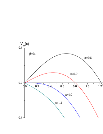
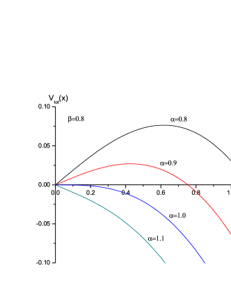
Figure 1: $V_{tot}(x)$ versus $x$. Left: $\beta=0.1$; Right: $\beta=0.8$. In all of the plots from top to bottom $\alpha=0.8,0.9,1.0,1.1$, respectively.

To show the effect of velocity on the potential barrier we plot $V_{tot}(x)$ against $x$ with $\alpha=0.9$ for different $\beta$ in the left panel of Fig.2. We can see that by increasing $\beta$ the height and width of the potential barrier both decrease. As we know the higher the potential barrier, the harder the produced pair escape to infinity. Therefore, the presence of velocity tends to increase the Schwinger effect.

To study how the velocity affects the value of $E_{c}$ we plot $V_{tot}(x)$ versus $x$ for different $\beta$ at $\alpha=1$ in the right panel of Fig.2. From the figures, we can see that the barrier vanishes for each plot implying the vacuum becomes unstable. Also, by increasing $\beta$ the height of the plot decreases, in agreement with the analysis of (34). Actually, that the barrier of each plot disappears at $\alpha=1$ can be strictly proved, i.e, one can calculate the $\frac{dV_{tot}(x)}{dx}$ at $x$ as

$$\frac{dV_{tot}}{dx}|_{x=0}=(1-\alpha)T_{F}\sqrt{f(r_{0})cosh^{2}\beta-sinh^{2}\beta}.$$ (37)

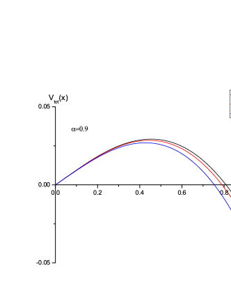
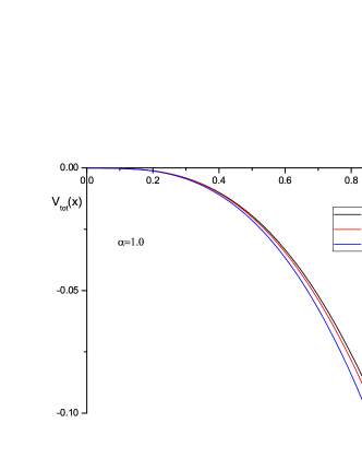
Figure 2: $V_{tot}(x)$ versus $x$. Left: $\alpha=0.9$; Right: $\alpha=1$. In all of the plots from top to bottom $\beta=0.1,0.5,0.8$, respectively.

III.2 Parallel to the wind $(\theta=0)$

We now discuss the system parallel to the wind. The coordinate is parameterized by

$$t=\tau,\qquad x_{1}=0,\qquad x_{2}=0,\qquad x_{3}=\sigma,\qquad r=r(\sigma).$$ (38)

where the test particles are located at $x_{3}=-\frac{x}{2}$ and $x_{3}=\frac{x}{2}$, respectively.

The next analysis is almost similar to the previous subsection. So we here show the final results. The total potential is given by

$$V_{tot}(x) = 2T_{F}r_{0}a\int_{1}^{1/a}dy\sqrt{\frac{A(y)B(y)}{A(y)-A(y_{c})}}$$ (39)

$$- \frac{2T_{F}\alpha r_{0}}{a}\sqrt{(f(r_{0})cosh^{2}\beta-sinh^{2}\beta)(cosh^{2}\beta-f(r_{0})sinh^{2}\beta)}\int_{1}^{1/a}dy\sqrt{\frac{A(y_{c})B(y)}{A^{2}(y)-A(y)A(y_{c})}}.$$

with

$$A(y)=y^{4}[f(y)(sinh^{4}\beta+cosh^{4}\beta)-(1+f^{2}(y))sinh^{2}\beta cosh^{2}\beta],\qquad B(y)=cosh^{2}\beta-\frac{1}{f(y)}sinh^{2}\beta,$$ (40)

and

$$A(y_{c})=f(y_{c})(sinh^{4}\beta+cosh^{4}\beta)-(1+f^{2}(y_{c}))sinh^{2}\beta cosh^{2}\beta.$$ (41)

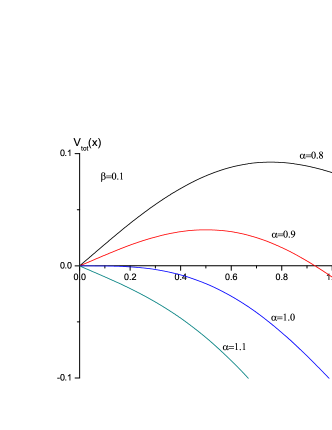
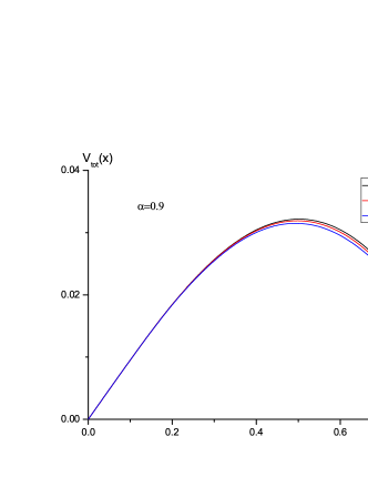
Figure 3: $V_{tot}(x)$ versus $x$. Left: $\beta=0.1$; from top to bottom $\alpha=0.8,0.9,1.0,1.1$, respectively. Right: $\alpha=0.9$, from top to bottom $\beta=0.1,0.5,0.8$, respectively.

In Fig.3, we also plot $V_{tot}(x)$ as a function of $x$ for $\theta=0$ in two cases. We can see that the behavior is similar to the case of $\theta=\pi/2$. The only difference is that $\beta$ has a smaller influence on the Schwinger effect when the pair is moving parallel to the plasma wind. Interestingly, the velocity also has a smaller influence on the imaginary potential MAL and the entropic force KBF when the pair moves parallel to the wind rather than transverse.

IV conclusion and discussion

In heavy ion collisions at LHC and RHIC, the produced pair is moving through the medium with relativistic velocities. An understanding of how some quantities are affected by the velocities may be essential for theoretical predictions. In this paper, we have investigated the influence of velocity on the Schwinger effect at finite temperature from the AdS/CFT correspondence. We have studied the pair moving transverse and parallel to the plasma wind respectively. The potential analysis for these backgrounds was presented. The value of the critical electric field was obtained. It is shown that for both cases the presence of velocity tends to increase the production rate. In addition, the velocity has a stronger influence on the Schwinger effect when the pair moves transverse to the plasma wind rather than parallel.

Finally, it is interesting to mention that the holographic Schwinger effect with a rotating D3-brane has been studied in HXU recently.

V Acknowledgments

This work is partly supported by the Ministry of Science and Technology of China (MSTC) under the 973 Project no. 2015CB856904(4). Zi-qiang Zhang and Gang Chen are supported by the NSFC under Grant no. 11475149. De-fu Hou is supported by the NSFC under Grant no. 11375070 and 11521064.

References

• (1) J. S. Schwinger, Phys. Rev. 82 (1951) 664.
• (2) I. K. Affleck and N. S. Manton, Nucl. Phys. B 194, 38 (1982).
• (3) E. S. Fradkin and A. A. Tseytlin, Nucl. Phys. B 261,1 (1985).
• (4) C. Bachas and M. Porrati, Phys. Lett. B 296 (1992) 77.
• (5) J. M. Maldacena, Adv. Theor. Math. Phys. 2, 231 (1998) [Int. J. Theor. Phys. 38, 1113 (1999).
• (6) S. S. Gubser, I. R. Klebanov and A. M. Polyakov, Phys. Lett. B428, 105 (1998).
• (7) O. Aharony, S. S. Gubser, J. Maldacena, H. Ooguri and Y. Oz, Phys. Rept. 323, 183 (2000).
• (8) G. W. Semenoff and K. Zarembo, Phys. Rev. Lett. 107 (2011) 171601.
• (9) Y. Sato and K. Yoshida, JHEP 1308 (2013) 002.
• (10) Y. Sato and K. Yoshida, JHEP 1312 (2013) 051.
• (11) Y. Sato and K. Yoshida, JHEP 1309 (2013) 134.
• (12) S. Bolognesi, F. Kiefer and E. Rabinovici, JHEP 1301 (2013) 174.
• (13) Y. Sato and K. Yoshida, JHEP 1304 (2013) 111.
• (14) S. Chakrabortty and B. Sathiapalan, Nucl. Phys. B 890 (2014) 241.
• (15) J. Ambjorn, Y. Makeenko, Phys. Rev. D 85, 061901 (2012) [hep-th/1112.5606].
• (16) K. Hashimoto, T. Oka, JHEP 10 (2013) 116.
• (17) D. D. Dietrich, Phys. Rev. D 90, 045024 (2014).
• (18) W. Fischler, P. H. Nguyen, J. F. Pedraza, W. Tangarife, Phys. Rev. D 91, 086015 (2015).
• (19) M. Ghodrati, Phys. Rev. D 92, 065015 (2015).
• (20) X. Wu, JHEP 09 (2015) 044.
• (21) Z.q.Zhang, D.f.Hou, Y.Wu and G.Chen, Advances in High Energy Physics, Volume 2016, Article ID 9258106.
• (22) D. Kawai, Y. Sato and K. Yoshida, Int. J. Mod. Phys. A 30, 1530026 (2015).
• (23) M. Ali-Akbari, D. Giataganas and Z. Rezaei, Phys. Rev. D 90 (2014) 086001.
• (24) K. B. Fadafan, S. K. Tabatabaei, Phys. Rev. D 94, 026007 (2016).
• (25) G. T. Horowitz and A. Strominger, Nucl. Phys. B 360 (1991) 197.
• (26) Barton Zwiebach. A first course in string theory, Cambridge university press, 2004.
• (27) H. Xu and Y.-Chang Huang, ITP No. 02, BJUT, [hep-th/1604.06331].