Hardware Impairments Aware Transceiver Design for Full-Duplex Amplify-and-Forward MIMO Relaying

Abstract

In this work we consider a full-duplex (FD) and amplify-and-forward (AF) relay with multiple antennas, where hardware impairments of the FD relay are taken into account. Due to the inter-dependency of the transmit relay power and the residual self-interference in an AF-FD relay, we observe a distortion loop that degrades the system performance when relay dynamic range is not high. In this regard, we analyze the relay function, and an optimization problem is formulated to maximize the signal to distortion-plus-noise ratio (SDNR) under relay and source transmit power constraints. Due to the problem complexity, we propose a gradient-projection-based (GP) algorithm to obtain an optimal solution. Moreover, a non-alternating sub-optimal solution is proposed by assuming a rank-1 relay amplification matrix, and separating the design of the relay process into multiple stages (MuStR1). The proposed MuStR1 method is then enhanced by introducing an alternating update over the optimization variables, denoted as AltMuStR1 algorithm. Numerical simulations show that compared to GP, the proposed (Alt)MuStR1 algorithms significantly reduce the required computational complexity at the expense of a slight performance degradation. Moreover, as the hardware impairments increase, or for a system with a high transmit power, the impact of applying a distortion-aware design is significant.

I Introduction

FULL-Duplex (FD) operation, as a transceiver’s capability to transmit and receive at the same time and frequency, is known with the potential to approach various requirements of future communication systems (5G), e.g., improved spectral efficiency and end-to-end latency [2]. Nevertheless, such systems have been long considered to be practically infeasible due to the inherent self-interference. In theory, since each node is aware of its own transmitted signal, the interference from the loopback path can be estimated and suppressed. However, in practice this procedure is challenging due to the high strength of the self-interference channel compared to the desired communication path, up to 100 dB [3]. Recently, specialized self-interference cancellation (SIC) techniques [4, 5, 6, 7] have provided an adequate level of isolation between transmit (Tx) and receive (Rx) directions to facilitate an FD communication and motivated a wide range of related applications, see, e.g., [2, 8]. A common idea of the such SIC techniques is to attenuate the main interference paths in RF domain, i.e., prior to down-conversion, so that the remaining self-interference can be processed in the effective dynamic range of the analog-to-digital convertor (ADC) and further attenuated in the baseband, i.e., digital domain. While the aforementioned SIC techniques have provided successful demonstrations for specific scenarios, e.g., [6], it is easy to observe that the obtained cancellation level may vary for different realistic conditions. This mainly includes i) aging and inaccuracy of the hardware components, e.g., ADC and digital-to-analog-convertor (DAC) noise, power amplifier and oscillator phase noise in analog domain, as well as ii) inaccurate estimation of the remaining interference paths due to the limited channel coherence time. As a result, it is essential to take into account the aforementioned inaccuracies to obtain a design which remains efficient under realistic situations.

In this work we are focusing on the application of FD capability on a classic relaying system, where the relay node has multiple antennas and suffers from the effects of hardware inaccuracy. An FD relay is capable of receiving the signal from the source, while simultaneously communicating to the destination. This capability, not only reduces the required time slots in order to accomplish an end to end communication, but also reduces the end to end latency compared to the known Time Division Duplex (TDD)-based half-duplex (HD) relays. In the early work by Riihonen. et. al. [9] the relay operation with a generic processing protocol is modeled, and many insights have been provided regarding the multiple-antenna strategies for reducing the self-interference power. The design methodologies and performance evaluation for FD relays with decode-and-forward (DF) operation have been then studied, see e.g., [10, 11, 12, 13, 14], taking into account the effects of the hardware impairments, as well as channel estimation errors in digital domain. For the FD relaying systems with amplify-and-forward (AF) operation, single antenna relaying scenarios are studied in [15, 16, 17, 18, 19, 20]. In the aforementioned works the effect of the linear inaccuracies in digital domain have been incorporated in [17], where the hardware imperfections from analog domain components have been addressed in [15, 16], following the model in [3, 10], and in [18] following the proposed model in [21]. The work in [18] is then extended by [19] to enhance the physical layer security in the presence of an Eavesdropper.

While the aforementioned literature introduces the importance of an accurate transceiver modeling with respect to the effects of hardware impairments for an FD-AF relay, such works are not yet extended for the relays with multiple antennas. This stems from the fact that in an FD-AF relay, the inter-dependent behavior of the transmit power from the relay and the residual self-interference intensity results in a distortion loop effect, see Subsection II-C. The aforementioned effect results in a rather complicated mathematical description when relay is equipped with multiple antennas. As a result, related studies resort to simplified models to reduce the consequent design complexity. In [22, 23, 24, 25, 26, 27, 28, 29, 30] a multiple-antenna FD-AF relay system is studied where a perfect SIC is assumed; via estimating and subtracting the interference in the receiver [22, 23, 24], or via spatial zero-forcing of the self-interference signal assuming that the number of transmit antennas exceeds the number of receive antennas at the relay [25, 26, 27, 28, 29, 30]. For the scenarios where the number of transmit antennas is not higher than the receive antennas, a general framework is proposed in [32, 31], assuming a fixed and known residual self-interference statistics, and in [33, 34], where a perfect SIC is assumed via a combined analog/digital SIC scheme, on the condition that the self-interference power does not exceed a certain threshold. In [35, 36] the residual self-interference signal is related to the transmit signal via a known and linear function, assuming a distortion-free hardware. A power adjustment method is proposed in [38] for an FD-AF relay equipped with a massive antenna array, by considering the impact of limited resolution ADCs in the end-to-end performance. However, the impact of the relay’s transmit/receive covariance on the residual self-interference is not considered. To the best of the authors knowledge, the impact of the hardware distortions, as such extensively studied for FD-DF relaying systems [10, 11, 12, 13, 14], is not yet addressed for multiple antenna FD-AF relays.

I-A Contribution

In this work, we study a multiple-input-multiple-output (MIMO) FD-AF relay, where the explicit impact of hardware distortions in the receiver and transmit chains are taken into account in the SIC process. Our goal is to enhance the instantaneous end-to-end performance via optimized linear transmit/receive strategies. The main contributions are as follows:

• Due to the joint consideration of hardware distortions in the receiver and transmit chains, we observe an inter-dependent behavior of the relay transmit covariance and the residual self-interference covariance in an FD-AF relay, i.e., the distortion loop effect. Note that this behavior may not be captured from the prior works based on simplified residual interference models, e.g., assuming a perfect SIC via estimation at the receiver [22]-[24], via transmit beamforming [25]-[30], assuming a known self-interference signal with perfect hardware [35], [36], or assuming a known (fixed) residual self-interference covariance [31]-[34]. In Section III, the relay operation is analyzed under the effect of distortion loop, and the instantaneous end-to-end signal-to-distortion-plus-noise ratio (SDNR) is formulated in relation to the statistics of the noise and hardware impairments.

• Building on the obtained analysis, we propose linear transmit/receive strategies with the intention of maximizing the SDNR. The instantaneous CSI is utilized to control the impact of distortion, and to enhance the quality of the desired signal. This is in contrast to [22, 23, 24, 25, 26, 27, 28, 29, 30, 33, 34, 32, 31] where the dependency of the distortion statistics to the intended transmit/receive signal is ignored, to [38] where a fixed transmit/receive strategy is assumed based on maximum ratio combining/transmission, or to [35, 36] where the residual self-interference channel is assumed to be a known design parameter. Note that the latter assumption is not practical, since the residual self-interference, by definition, is unknown to the receiver. In this regard, an SDNR maximization problem is formulated which shows an intractable mathematical structure due to impact of the distortion loop. A gradient-projection (GP) based solution is then proposed in Section IV to act as a benchmark for the achievable performance, however, imposing a high computational complexity.

• In order to reduce the design computational complexity, a sub-optimal Multi-Stage Rank-1 (MuStR1) solution is introduced in Section V, by assuming a rank-1 relay amplification matrix and separating the design of the relay process into multiple stages. In this regard, a non-alternating algorithm is proposed by locally maximizing the resulting SDNR for each stage. Moreover, the performance of MuStR1 is improved by introducing an alternating update (AltMuStR1) at the cost of a slightly higher computational complexity compared to MuStR1. Similar to the previous parts, this approach differs from the rank-1 FD-AF relaying schemes proposed in [33, Subsection 3.2] and [30, Section III], where the impact of distortions are not considered in the design of transmit/receive strategies.

Numerical simulations show that for a system with a small thermal noise variance, or a high power or transceiver inaccuracy, the application of a distortion-aware design is essential.

I-B Mathematical Notation:

Throughout this paper, column vectors and matrices are denoted as lower-case and upper-case bold letters, respectively. The rank of a matrix, expectation, trace, transpose, conjugate, Hermitian transpose, determinant and Euclidean norm are denoted by ${\text{rank}}(\cdot),\;\mathbb{E}(\cdot),\;{\text{ tr}}(\cdot),\;(\cdot)^{T}$, $(\cdot)^{*}$, $(\cdot)^{H},\;|\cdot|,\;||\cdot||_{2}$, respectively. The Kronecker product is denoted by $\otimes$. The identity matrix with dimension $K$ is denoted as ${\mathbf{I}}_{K}$ and ${\text{vec}}(\cdot)$ operator stacks the elements of a matrix into a vector, and $(\cdot)^{-1}$ represents the inverse of a matrix. The sets of real, real and positive, complex, natural, and the set $\{1\ldots K\}$ are respectively denoted by , ⁺, $\mathbb{C}$, $\mathbb{N}$ and $\mathbb{F}_{K}$. $\left\lfloor\mathbf{A}_{i}\right\rfloor_{i\in\mathbb{F}_{K}}$ denotes a tall matrix, obtained by stacking the matrices $\mathbf{A}_{i},~{}i\in\mathbb{F}_{K}$. The set of all positive semi-definite matrices is denoted by $\mathcal{H}$. $\bot$ represents statistical independence. $\mathbf{\lambda}_{\text{max}}(\mathbf{A})$ calculates the dominant eigenvector of $\mathbf{A}$. $x^{\star}$ is the value of the variable $x$ at optimality.

II System Model

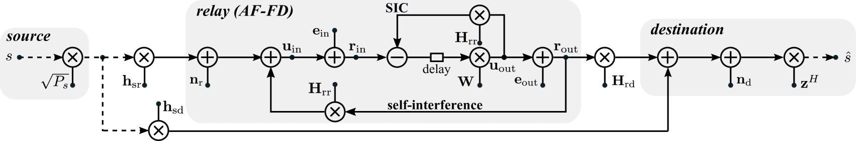
Figure 1: The signal model in an amplify-and-forward FD MIMO relay. The impact of hardware inaccuracies form the transmitter ($\mathbf{e}_{\text{out}}$) and receiver ($\mathbf{e}_{\text{in}}$) chains is observable on the relay process. The bold arrows represent the vector signals while the dashed arrows represent the scalars. See Section II for a detailed description.

We investigate a system where a single-antenna HD source communicates with an HD destination node equipped with $M_{\text{d}}$ antennas, with a help of an FD relay. The relay is assumed to have $M_{\text{t}}$ ($M_{\text{r}}$) transmit (receive) antennas, and operates in AF mode. The channels between the source and the relay, between the relay and the destination, and between the source and the destination are denoted as $\mathbf{h}_{\text{sr}}\in\mathbb{C}^{M_{\text{r}}}$, $\mathbf{H}_{\text{rd}}\in\mathbb{C}^{M_{\text{d}}\times M_{\text{t}}}$, and $\mathbf{h}_{\text{sd}}\in\mathbb{C}^{M_{\text{d}}}$, respectively. The self-interference channel, which is the channel between the relay’s transmit and receive ends is denoted as $\mathbf{H}_{\text{rr}}\in\mathbb{C}^{M_{\text{r}}\times M_{\text{t}}}$. All channels are following the flat-fading model.

II-A Source-to-Relay Communication

The relay continuously receives and amplifies the received signal from the source, while estimating and subtracting the loopback self-interference signal from its own transmitter, see Fig. 1. The received signal at the relay is expressed as

$$\mathbf{r}_{{\text{in}}}=\underbrace{\mathbf{h}_{{\text{sr}}}\sqrt{P_{\text{s}}}s+\mathbf{H}_{{\text{rr}}}\mathbf{r}_{{\text{out}}}+\mathbf{n}_{\text{r}}}_{=:\mathbf{u}_{\text{in}}}+\mathbf{e}_{{\text{in}}},$$ (1)

where $\mathbf{r}_{{\text{in}}}\in\mathbb{C}^{M_{\text{r}}}$ and $\mathbf{r}_{{\text{out}}}\in\mathbb{C}^{M_{\text{t}}}$ respectively represent the received and transmitted signal from the relay and $\mathbf{n}_{\text{r}}\sim\mathcal{CN}\left(\mathbf{0},\sigma_{\text{nr}}^{2}\mathbf{I}_{{M_{\text{r}}}}\right)$ represents the zero-mean additive white complex Gaussian (ZMAWCG) noise at the relay. The transmitted data symbol from the source is denoted as $s\in\mathbb{C}$, $\mathbb{E}\{|s|^{2}\}=1$. $P_{\text{s}}\in^{+}$ is the source transmit power and ${\mathbf{u}_{{\text{in}}}}\in\mathbb{C}^{M_{\text{r}}}$ represents the undistorted received signal at the relay.

The receiver distortion, denoted as $\mathbf{e}_{{\text{in}}}\in\mathbb{C}^{M_{\text{r}}}$, represents the combined effects of receiver chain impairments, e.g., limited ADC accuracy, oscillator phase noise, low-noise-amplifier (LNA) distortion [10]. Please note that while the aforementioned impairments are usually assumed to be ignorable for an HD transceiver, they play an important role in our system due to high strength of the self-interference path. The known, i.e., distortion-free, part of the self-interference signal is then suppressed in the receiver by utilizing the recently developed SIC techniques in analog and digital domains, e.g., [4, 6]. The remaining signal is then amplified to constitute the relay’s output:

$$\mathbf{r}_{{\text{out}}} =\mathbf{u}_{\text{out}}+\mathbf{e}_{{\text{out}}},\;\;\mathbf{u}_{{\text{out}}}(t)=\mathbf{W}\mathbf{r}_{{\text{supp}}}(t-\tau),$$ (2)

$$\mathbf{r}_{{\text{supp}}} =\mathbf{r}_{{\text{in}}}-{\mathbf{H}}_{{\text{rr}}}\mathbf{u}_{{\text{out}}},$$ (3)

where $\mathbf{r}_{{\text{supp}}}\in\mathbb{C}^{M_{\text{r}}}$ and $\mathbf{W}\in\mathbb{C}^{{M_{\text{t}}}\times{M_{\text{r}}}}$ respectively represent the interference-suppressed version of the received signal and the relay amplification matrix, $t\in^{+}$ represents the time instance, and $\tau\in^{+}$ is the relay processing delay, see Subsection II-E4. The intended transmit signal is denoted as $\mathbf{u}_{{\text{out}}}\in\mathbb{C}^{M_{\text{t}}}$. Similar to the defined additive distortion in the receiver chains, the combined effects of the transmit chain impairments, e.g., limited DAC accuracy, oscillator phase noise, power amplifier noise, is denoted by $\mathbf{e}_{{\text{out}}}\in\mathbb{C}^{M_{\text{r}}}$. Furthermore, in order to take into account the transmit power limitations we impose

$$\mathbb{E}\{\|\mathbf{r}_{{\text{out}}}\|_{2}^{2}\}\leq P_{\text{r,max}},\;P_{\text{s}}\leq P_{\text{s,max}},$$ (4)

where $P_{\text{r,max}}$ and $P_{\text{s,max}}$ respectively represents the maximum transmit power from the relay and from the source.

II-B Distortion signal statistics

The impact of hardware elements inaccuracy in each chain is modeled as additive distortion terms, following the FD transceiver model proposed in [3] and widely used in the context of FD system design and performance analysis, e.g., [10, 11, 12, 13, 14]. The proposed model in [3] is based on the following three observations. Firstly, the collective distortion signal in each transmit/receive chain can be approximated as an additive zero-mean Gaussian term [39, 41, 40]. Secondly, the variance of the distortion signal is proportional to the power of the intended transmit/received signal. And third, the distortion signal is statistically independent to the intended transmit/receive signal at each chain, and for different chains. Please note that the the statistical independence of distortion elements holds also for an advanced implementation of an FD transceiver, assuming a high signal processing capability. This is since, any known correlation can be constructively used, and hence eliminated, to reduce the residual self-interference. However, the linear dependence of the remaining distortion signal to the signal strength varies for different SIC techniques and is considered as an approximation, see [3, Subsections C] for further elaboration on the used model. In the defined relaying system it is expressed as

$$\mathbf{e}_{{\text{in}}}\sim\mathcal{CN} \Big{(}\mathbf{0},\beta\text{diag}\Big{(}\mathbb{E}\left\{\mathbf{u}_{\text{in}}\mathbf{u}_{\text{in}}^{{H}}\right\}\Big{)}\Big{)},$$

$$\mathbf{e}_{{\text{in}}}({t})\bot\mathbf{e}_{{\text{in}}}({{t}^{{}^{\prime}}}),\;\;\mathbf{e}_{{\text{in}}}({t})\bot\mathbf{u}_{{\text{in}}}({t}),$$ (5)

and

$$\mathbf{e}_{{\text{out}}}\sim\mathcal{CN} \Big{(}\mathbf{0},{{\color[rgb]{0,0,0}\kappa}}\text{diag}\Big{(}\mathbb{E}\left\{\mathbf{u}_{\text{out}}\mathbf{u}_{\text{out}}^{{H}}\right\}\Big{)}\Big{)},$$

$$\mathbf{e}_{{\text{out}}}({t})\bot\mathbf{e}_{{\text{out}}}({{t}^{{}^{\prime}}}),\;\;\mathbf{e}_{{\text{out}}}({t})\bot\mathbf{u}_{{\text{out}}}({t}),$$ (6)

where ${t}\neq{{t}^{{}^{\prime}}}$ and $\beta,\kappa\in^{+}$ are the receive and transmit distortion coefficients which respectively relate the undistorted receive and transmit signal covariance to the covariance of the corresponding distortion. It is worth mentioning that the values of $\kappa,\beta$ depend of the implemented SIC scheme, and reflect the quality of the cancellation. For instance, for an FD massive MIMO system where analog cancelers are not used due to complexity, and the resolution of the ADC/DAC are limited to reduce the cost, the values of $\kappa,\beta$ can be determined by the used quantization bits, e.g., $\kappa\approx-6\times b$ dB, for a uniform DAC quantization with $b$ bits. However, in general, the choice of $\kappa,\beta$ depend on the implemented SIC and the used analog circuitry, e.g., the number of delay taps implemented in [6, Subsection 3.1]. Note that the defined statistics in (5), (6) indicate that unlike the traditional additive white noise model, a higher transmit (receive) signal power results in a higher transmit (receive) distortion intensity in the corresponding chain. As we will further elaborate, this effect plays an important role in the performance of an FD-AF relay. For more discussions on the used distortion model please see [3, 10, 12, 11], and the references therein.

II-C Relay-to-destination communication

The transmitted signal from the relay node passes through the relay to destination channel and constitutes the received signal at the destination:

$$\mathbf{y} =\mathbf{H}_{{\text{rd}}}\mathbf{r}_{{\text{out}}}+\mathbf{h}_{{\text{sd}}}\sqrt{P_{\text{s}}}s+\mathbf{n}_{\text{d}},\;\;\hat{s}(t-\tau)=\mathbf{z}^{{H}}\mathbf{y}(t),$$ (7)

where $\mathbf{y}\in\mathbb{C}^{M_{\text{d}}}$ is the received signal at the destination, and $\mathbf{n}_{\text{d}}\sim\mathcal{CN}\left(\mathbf{0},\sigma_{\text{nd}}^{2}{\mathbf{I}}_{M_{\text{d}}}\right)$ is the ZMAWCG noise. The linear receiver filter and the estimated received symbol is denoted as $\mathbf{z}\in\mathbb{C}^{M_{\text{{d}}}}$ and $\hat{s}$, respectively. Please see Table I for the list of used signal notations and system parameters.

TABLE I: Used signal notations and system parameters

Deterministic Param.	Description
$\mathbb{S}_{d}$	Set of all deterministic parameters
$\mathbf{H}_{\text{rr}}$	Instantaneous relay-relay channel
$\mathbf{H}_{\text{rd}}$	Instantaneous relay-destination channel
$\mathbf{h}_{\text{sr}}(\mathbf{h}_{\text{sd}})$	Instantaneous source-relay (destination) channel
$P_{\text{s,max}}(P_{\text{r,max}})$	Maximum transmit power at the source (relay)
$\sigma_{\text{nr}}^{2}(\sigma_{\text{nd}}^{2})$	Thermal noise variance at the relay (destination)
$\kappa(\beta)$	Distortion coefficients for the transmit (receive) chains
Random Param.	Description
$\mathbb{S}_{r}$	Set of all random parameters
$s$	Transmit data symbol from source
$\mathbf{n}_{\text{r}}(\mathbf{n}_{\text{d}})$	Thermal noise at the relay (destination)
$\mathbf{e}_{\text{in}}(\mathbf{e}_{\text{out}})$	Receive (transmit) distortion at the relay

II-D Distortion loop

As the transmit power from the relay increases, the power of the error components increase in all receiver chains, see (1) in connection to (5)-(6). On the other hand, these errors are amplified in the relay process and further increase the relay transmit power, see (1) in connection to (3) and (2). The aforementioned effect causes a loop which signifies the problem of residual self-interference for the relays with AF process. In the following section, this impact is analytically studied and an optimization strategy is proposed in order to alleviate this effect.

II-E Remarks

II-E1 CSI estimation

In this work we assume that the channel state information (CSI), representing linear signal dependencies in the system, are known by dedicating an adequately long training sequence at the relay. Therefore, the studied framework serves best for the scenarios with a stationary channel where long training sequences can be utilized, e.g., relay channel in a static backhaul link with a directive line-of-sight (LOS) connection [42]. Note that the acquisition of an accurate CSI is challenging due to noise, interference, as well as the impact of hardware impairments. However, an effective estimation method is presented in [10, Subsection III.A] for an FD relaying setup in the presence of hardware impairments. It is observed that an accurate CSI can be obtained on the condition of employing a sufficiently long training sequence, see [10, Equation (9)], and also [3, Equation (10)] for a similar argument. For the scenarios where the CSI can not be accurately obtained, the results of this paper can be treated as theoretical guidelines on the effects of hardware impairments, if CSI were accurately known.

II-E2 Hardware impairments

Compared to many HD scenarios the impact of hardware impairments is severe in FD transceivers due to the strong self-interference, see, e.g., specifications of SIC for 802.11ac PHY [6]. This is since on one hand, the distortions originating from the transmit chains pass through a strong self-interference channel and become significant. On the other hand, the receiver chains are more prone to distortion due to the high-power received signal. In this work, we focus on the impact of hardware impairments for the FD relay transceiver, and otherwise model the inaccuracies as an additive thermal noise.

II-E3 Direct link

In this work, we assume that the direct link is weak and consider the source-destination path as a source of interference, similar to [17, 10]. For the scenarios where the direct link is strong, it is shown in [43] that the receiver strategy can be gainfully updated as a RAKE receiver [44] to temporally align the desired signal in the direct and relay links. This can be considered as a future extension of the current work.

II-E4 Processing delay

The relay output signals, i.e., $\mathbf{u}_{{\text{out}}}$ and $\mathbf{r}_{{\text{out}}}$, are generated from the received signals with a relay processing delay $\tau$, see (2). This delay is assumed to be long enough, e.g., more than a symbol duration, such that the source signal is decorelated, i.e., $s(t)\bot s(t-\tau)$ [43, 45]. The zero-mean and independent statistics of the samples from data signal, i.e., $s(t)$ and $s(t-\tau)$, as well as the noise and distortion signals, are basis for the analysis in the following section.

III Performance Analysis for MIMO AF Relaying with Hardware Impairments

In this part, we analyze the end-to-end performance as a function of the relay amplification matrix, i.e., $\mathbf{W}$, receive linear filter at the destination, i.e., $\mathbf{z}$, as well as the transmit power from the source, $P_{\text{s}}$. By incorporating (1) and (5)-(6) into (2) and (3) we have

$$\mathbf{Q}=\mathbf{W}\Big{(}P_{\text{s}}\mathbf{h}_{{\text{sr}}}\mathbf{h}_{{\text{sr}}}^{{H}} +\sigma_{\text{nr}}^{2}\mathbf{I}_{{M_{\text{r}}}}+\mathbb{E}\left\{\mathbf{e}_{\text{in}}\mathbf{e}_{\text{in}}^{{H}}\right\}$$

$$+{\mathbf{H}}_{{\text{rr}}}\mathbb{E}\{\mathbf{e}_{{\text{out}}}\mathbf{e}_{{\text{out}}}^{{H}}\}{\mathbf{H}}_{{\text{rr}}}^{{H}}\Big{)}\mathbf{W}^{{H}}$$

$$=\mathbf{W}\Big{(}P_{\text{s}}\mathbf{h}_{{\text{sr}}}\mathbf{h}_{{\text{sr}}}^{{H}} +\sigma_{\text{nr}}^{2}\mathbf{I}_{{M_{\text{r}}}}+\beta\text{diag}\big{(}\mathbb{E}\left\{\mathbf{u}_{\text{in}}\mathbf{u}_{\text{in}}^{{H}}\right\}\big{)}$$

$$+\kappa{\mathbf{H}}_{{\text{rr}}}\text{diag}\big{(}\mathbf{Q}\big{)}{\mathbf{H}}_{{\text{rr}}}^{{H}}\Big{)}\mathbf{W}^{{H}},$$ (8)

where $\mathbf{Q}\in\mathcal{H}$ is the covariance matrix of the undistorted transmit signal from the relay, i.e., $\mathbf{Q}:=\mathbb{E}\{\mathbf{u}_{{\text{out}}}\mathbf{u}_{{\text{out}}}^{{H}}\}$. Furthermore, the undistorted receive covariance matrix can be formulated from (1)-(3) as

$$\mathbb{E}\{\mathbf{u}_{{\text{in}}}\mathbf{u}_{{\text{in}}}^{{H}}\} =P_{\text{s}}\mathbf{h}_{{\text{sr}}}\mathbf{h}_{{\text{sr}}}^{{H}}+\sigma_{\text{nr}}^{2}\mathbf{I}_{{M_{\text{r}}}}+{\mathbf{H}}_{{\text{rr}}}\mathbb{E}\{\mathbf{r}_{{\text{out}}}\mathbf{r}_{{\text{out}}}^{{H}}\}{\mathbf{H}}_{{\text{rr}}}^{{H}}.$$ (9)

It is worth mentioning that due to the proximity of the Rx and Tx antennas on the FD device, the loopback self-interference signal is much stronger than the desired signal which is coming from a distant location, and hence constitutes the principle part in (9). By recalling (2) and (6) the relay transmit covariance matrix can be formulated as

$$\mathbb{E}\{\mathbf{r}_{{\text{out}}}\mathbf{r}_{{\text{ out}}}^{{H}}\}=\mathbf{Q}+\kappa\text{diag}\left(\mathbf{Q}\right),$$ (10)

and consequently from (III) and (9) it follows

$$\mathbf{Q}=\mathbf{W}\mathcal{R}\left(\mathbf{Q}\right)\mathbf{W}^{H},$$ (11)

where

$$\mathcal{R}\left(\mathbf{Q}\right):=P_{\text{s}}\mathbf{h}_{{\text{sr}}}\mathbf{h}_{{\text{ sr}}}^{{H}} +\sigma_{\text{nr}}^{2}\mathbf{I}_{{M_{\text{ r}}}}+\beta\text{diag}\left(P_{\text{s}}\mathbf{h}_{{\text{sr}}}\mathbf{h}_{{\text{sr}}}^{{H}}+\sigma_{\text{nr}}^{2}\mathbf{I}_{{M_{\text{r}}}}\right)$$

$$+\beta\text{diag}\Big{(}{\mathbf{H}}_{{\text{rr}}}\Big{(}\mathbf{Q}+\kappa\text{diag}\left(\mathbf{Q}\right)\Big{)}{\mathbf{H}}_{{\text{rr}}}^{{H}}\Big{)}$$

$$+\kappa{\mathbf{H}}_{{\text{rr}}}\text{diag}\left(\mathbf{Q}\right){\mathbf{H}}_{{\text{ rr}}}^{{H}}.$$ (12)

Note that the above derivations (III)-(11) hold as the noise, the desired signal at subsequent symbol durations, and the distortion components are zero-mean and mutually independent. Unfortunately, a direct expression of $\mathbf{Q}$ in terms of $\mathbf{W}$ can not be achieved from (11), (III) in the current form. In order to facilitate further analysis we resort to the vectorized presentation of $\mathbf{Q}$. By applying the famous matrix equality $\text{vec}(\mathbf{A}_{1}\mathbf{A}_{2}\mathbf{A}_{3})=(\mathbf{A}_{3}^{\text{T}}\otimes\mathbf{A}_{1})\text{vec}(\mathbf{A}_{2})$, we can write (10) as

$$\text{vec}\left(\mathbb{E}\{\mathbf{r}_{{\text{out}}}\mathbf{r}_{{\text{out}}}^{{H}}\}\right)=\left(\mathbf{I}_{M_{\text{t}}^{2}}+\kappa\mathbf{S}_{\text{D}}^{M_{\text{t}}}\right)\text{vec}\left(\mathbf{Q}\right),$$ (13)

where $\mathbf{S}_{\text{D}}^{M}\in\{0,1\}^{{M^{2}}\times{M^{2}}}$ is a selection matrix with one or zero elements such that $\mathbf{S}_{\text{D}}^{M_{\text{t}}}\text{vec}\left(\mathbf{Q}\right)=\text{vec}\left(\text{diag}(\mathbf{Q})\right)$. Similarly from (11) we obtain

$$\text{vec}\left(\mathbf{Q}\right) =\Big{(}\mathbf{I}_{M_{\text{t}}^{2}}-\left(\mathbf{W}^{*}\otimes\mathbf{W}\right)\mathbf{C}\Big{)}^{-1}\left(\mathbf{W}^{*}\otimes\mathbf{W}\right)\mathbf{c},$$ (14)

where

$$\mathbf{C}: =\beta\mathbf{S}_{\text{D}}^{M_{\text{r}}}\left({\mathbf{H}}_{{\text{rr}}}^{*}\otimes{\mathbf{H}}_{{\text{ rr}}}\right)\left(\mathbf{I}_{M_{\text{t}}^{2}}+\kappa\mathbf{S}_{\text{D}}^{M_{\text{t}}}\right)+\kappa\left({\mathbf{H}}_{{\text{rr}}}^{*}\otimes{\mathbf{H}}_{{\text{rr}}}\right)\mathbf{S}_{\text{D}}^{M_{\text{t}}},$$ (15)

$$\mathbf{c}: =\left(\mathbf{I}_{M_{\text{r}}^{2}}+\beta\mathbf{S}_{\text{D}}^{M_{\text{r}}}\right)\text{vec}\left(P_{\text{s}}\mathbf{h}_{{\text{sr}}}\mathbf{h}_{{\text{sr}}}^{{H}}+\sigma_{\text{nr}}^{2}\mathbf{I}_{{M_{\text{r}}}}\right).$$ (16)

The direct dependence of the relay transmit covariance matrix and $\mathbf{W}$ can be consequently obtained from (14) and (13) as

$$\text{vec}\left(\mathbb{E}\{\mathbf{r}_{{\text{out}}}\mathbf{r}_{{\text{out}}}^{{H}}\}\right)=\mathbf{\Theta}\big{(}\mathbf{W},\mathbf{H}_{\text{rr}},\kappa,\beta\big{)}\text{vec}\left(P_{\text{s}}\mathbf{h}_{{\text{sr}}}\mathbf{h}_{{\text{sr}}}^{{H}}+\sigma_{\text{nr}}^{2}\mathbf{I}_{{M_{\text{r}}}}\right)$$ (17)

such that

$$\mathbf{\Theta}\big{(}\mathbf{W},\mathbf{H}_{\text{rr}},\kappa,\beta\big{)}:=\left(\mathbf{I}_{M_{\text{t}}^{2}}+\kappa\mathbf{S}_{\text{D}}^{M_{\text{t}}}\right)\Big{(}\mathbf{I}_{M_{\text{t}}^{2}}-\left(\mathbf{W}^{*}\otimes\mathbf{W}\right)\mathbf{C}\Big{)}^{-1}$$

$$\;\;\;\;\;\;\;\;\;\;\;\;\;\;\;\;\;\;\;\;\;\times\left(\mathbf{W}^{*}\otimes\mathbf{W}\right)\left(\mathbf{I}_{M_{\text{r}}^{2}}+\beta\mathbf{S}_{\text{D}}^{M_{\text{r}}}\right)$$ (18)

represents the transfer function of the relay; relating the distortion-less input, i.e., $P_{\text{s}}\mathbf{h}_{{\text{sr}}}\mathbf{h}_{{\text{sr}}}^{{H}}+\sigma_{\text{nr}}^{2}\mathbf{I}_{{M_{\text{r}}}}$, to the distorted transmit covariance. It can be observed that $\mathbf{\Theta}\left(\mathbf{W},\mathbf{H}_{\text{rr}},0,0\right)=\mathbf{W}^{*}\otimes\mathbf{W}$, which is similar to the known FD-AF relay operation with a perfect hardware, i.e., $\kappa,\beta=0$.

III-A Optimization problem

In order to formulate the end-to-end link quality, we recall that the noise, the desired signal and the residual interference signals are zero-mean and mutually independent. Hence, the received signal power at the destination, after application of $\mathbf{z}$, can be separated as

$$P_{\text{des}} ={\color[rgb]{0,0,0}\mathbb{E}_{\mathbb{S}_{r}}}\left\{\left|\mathbf{z}^{{H}}\mathbf{H}_{{\text{rd}}}\mathbf{W}\mathbf{h}_{{\text{sr}}}\sqrt{P_{s}}s\right|^{2}\right\}$$

$$=P_{s}\mathbf{z}^{{H}}\mathbf{H}_{{\text{rd}}}\mathbf{W}\mathbf{h}_{{\text{sr}}}\mathbf{h}_{{\text{sr}}}^{{H}}\mathbf{W}^{{H}}\mathbf{H}_{{\text{rd}}}^{{H}}\mathbf{z},$$ (19)

$$P_{\text{tot}} ={\color[rgb]{0,0,0}\mathbb{E}_{\mathbb{S}_{r}}}\left\{\left|\mathbf{z}^{{H}}\left(\mathbf{H}_{{\text{rd}}}\mathbf{r}_{\text{out}}+\mathbf{h}_{{\text{sd}}}\sqrt{P_{s}}s+\mathbf{n}_{\text{d}}\right)\right|^{2}\right\}=$$

$$\mathbf{z}^{{H}}\left(\mathbf{H}_{{\text{rd}}}\Big{(}\mathbf{Q}+\kappa\text{diag}\left(\mathbf{Q}\right)\Big{)}\mathbf{H}_{{\text{ rd}}}^{{H}}+\sigma_{\text{nd}}^{2}\mathbf{I}_{M_{\text{d}}}+P_{\text{s}}\mathbf{h}_{{\text{sd}}}\mathbf{h}_{{\text{sd}}}^{H}\right)\mathbf{z},$$ (20)

$$P_{\text{err}} =P_{\text{tot}}-P_{\text{des}},$$ (21)

where ${\mathbb{E}_{\mathbb{S}_{r}}}$ is the statistical expectation over the set of random variables $\mathbb{S}_{r}$, see Table I. Moreover, $P_{\text{des}}$ and $P_{\text{err}}$ respectively represent the power of the desired, and distortion-plus-noise parts of the estimated signal $\hat{\mathbf{s}}$, and $P_{\text{tot}}:=\mathbb{E}\{|\hat{{s}}|^{2}\}$. It is worth mentioning that $P_{\text{tot}}\geq P_{\text{des}}$, and hence $P_{\text{err}}\geq 0$, due to the superposition of the statistically independednt noise, distortion, and signal terms at different nodes or time instances. The corresponding optimization problem for maximizing the resulting SDNR is written as

$$\underset{P_{\text{s}},\mathbf{z},\mathbf{W}}{\text{max}}\;\;\; \frac{P_{\text{des}}}{P_{\text{err}}}$$ (22a)

s.t. $$(\ref{eq_loop_vec_U_out}),\;\;\mathbf{Q}\in\mathcal{H},\;\;\text{tr}\left(\mathbf{Q}\right)\leq\tilde{P}_{\text{r,max}},\;\;0\leq P_{\text{s}}\leq P_{\text{s,max}},$$ (22b)

where (22b) limits the feasible set of $\mathbf{W}$ to those resulting in a feasible $\mathbf{Q}$. Note that $\tilde{P}_{\text{r,max}}:=\frac{{P}_{\text{r,max}}}{1+\kappa}$, and the power constraint in (22b) follows as $\text{tr}\left(\mathbf{Q}+\kappa\text{diag}(\mathbf{Q})\right)=(1+\kappa)\text{tr}\left(\mathbf{Q}\right)$.

As it can be observed, the optimization problem (22a)-(22b) is a non-convex optimization problem and cannot be solved analytically, due to the structure imposed by (14). In order to approach the solution, we propose a GP-based optimization method in the following section.

IV Gradient Projection (GP) for SDNR maximization

In this part we propose an iterative solution to (22a)-(22b) based on the gradient projection method [46, 3]. In this regard, the optimization variables are updated in the increasing direction of the objective function (22a).

IV-A Iterative update for $\mathbf{W}$

The update rule for $\mathbf{W}$ is defined following the GP method, where detailed instructions are inspired from [10]. This includes the update of $\mathbf{W}$ in the steepest ascent direction, and occasional projection due to constraints violation. This is expressed as

$$\bar{\mathbf{W}}^{[l]} =\mathcal{P}\left(\mathbf{W}^{[l]}+\delta^{[l]}\nabla\left(\text{SDNR}\right)\right)$$

$$\mathbf{W}^{[l+1]} =\mathbf{W}^{[l]}+\gamma^{[l]}\left(\bar{\mathbf{W}}^{[l]}-{\mathbf{W}}^{[l]}\right),$$ (23)

where $\mathcal{P}\left(\cdot\right)$ represents the projection to the feasible solution space, $l$ is the iteration index, $\nabla\left(\cdot\right)$ represents the gradient with respect to $\mathbf{W}^{*}$, and $\delta,\gamma\in^{+}$ represent the step size variables. The update direction is obtained from the calculated gradients in (25)-(26), and the fact that

$$\nabla\left(\text{SDNR}\right)=\Big{(}\nabla\left({P_{\text{des}}}\right){P_{\text{err}}}-\nabla\left({P_{\text{err}}}\right){P_{\text{des}}}\Big{)}/{{P_{\text{err}}}^{2}}.$$ (24)

The stepsize value $\gamma$ is chosen according to the Armijo’s step size rule [47]. This is expressed as

$$\text{SDNR}\left(\mathbf{W}^{[l+1]}\right)-\text{SDNR}\left(\mathbf{W}^{[l]}\right)$$

$$\geq\sigma\nu^{m}\text{tr}\left(\Big{\{}\nabla\left(\text{SDNR}\right)\Big{\}}^{H}\left(\bar{\mathbf{W}}^{[l]}-{\mathbf{W}}^{[l]}\right)\right),$$

where $\gamma^{[l]}=\nu^{m}$, such that $m$ is the smallest non-negative integer satisfying the above inequality, and $\nu=0.5$, $\sigma=0.1$ and $\delta=1$.

$$\text{vec}\left(\nabla{P_{\text{err}}}\right)^{{T}} =\text{vec}\left(\left(\mathbf{H}_{\text{rd}}^{{H}}\mathbf{z}\mathbf{z}^{{H}}\mathbf{H}_{\text{rd}}\right)^{{T}}\right)^{{T}}\left(\mathbf{I}_{M_{\text{t}}^{2}}+\kappa\mathbf{S}_{\text{D}}^{M_{\text{t}}}\right)\Bigg{(}\left[\mathbf{c}+\mathbf{C}\big{(}\mathbf{I}_{M_{\text{t}}^{2}}-\left(\mathbf{W}^{*}\otimes\mathbf{W}\right)\mathbf{C}\big{)}^{-1}\left(\mathbf{W}^{*}\otimes\mathbf{W}\right)\mathbf{c}\right]^{{T}}\$$

$$\otimes\big{(}\mathbf{I}_{M_{\text{t}}^{2}}-\left(\mathbf{W}^{*}\otimes\mathbf{W}\right)\mathbf{C}\big{)}^{-1}\Bigg{)}{\mathbf{S}}_{\text{K}}\left(\mathbf{w}\otimes\mathbf{I}_{M_{\text{r}}M_{\text{t}}}\right)-\left(\mathbf{z}^{{T}}\mathbf{H}_{\text{rd}}^{\text{*}}\right)\otimes\left(P_{\text{s}}\mathbf{z}^{{H}}\mathbf{H}_{\text{rd}}\mathbf{W}\mathbf{h}_{\text{sr}}\mathbf{h}_{\text{sr}}^{{H}}\right){\mathbf{S}}_{\text{T}},$$ (25)

$$\text{vec}\left(\nabla{P_{\text{des}}}\right)^{{T}} =\left(\mathbf{z}^{{T}}\mathbf{H}_{\text{rd}}^{\text{*}}\right)\otimes\left(P_{\text{s}}\mathbf{z}^{{H}}\mathbf{H}_{\text{rd}}\mathbf{W}\mathbf{h}_{\text{sr}}\mathbf{h}_{\text{sr}}^{{H}}\right){\mathbf{S}}_{\text{T}},\;\;\text{where}\;\;\mathbf{w}:=\text{vec}(\mathbf{W}),\;{\mathbf{S}}_{\text{K}}\in\{0,1\}^{M_{\text{r}}^{2}M_{\text{t}}^{2}\times M_{\text{r}}^{2}M_{\text{t}}^{2}},\;{\mathbf{S}}_{{\text{T}}}\in\{0,1\}^{M_{\text{r}}M_{\text{t}}\times M_{\text{r}}M_{\text{t}}},$$ (26)

such that: $$\;\text{vec}\left(\mathbf{W}^{*}\otimes\mathbf{W}\right)={\mathbf{S}}_{\text{K}}\text{vec}\left(\mathbf{w}^{*}\mathbf{w}^{{T}}\right),\;\;\text{and}\;\;{\mathbf{S}}_{{\text{T}}}\text{vec}(\mathbf{W})=\text{vec}(\mathbf{W}^{{T}}).$$ (27)

IV-A1 Projection rule

Once an updated ${\mathbf{W}}$, and the corresponding $\mathbf{Q}$ calculated from (14), violate the problem constrains, i.e., when $\mathbf{Q}$ contains a negative eigenvalue or exceeds the defined power constraint, see (22b), it is projected in to the feasible variable space. Due to the convexity of the feasible variable space in $\mathbf{Q}$, similar to the suggested procedure in [55], we follow a projection rule which results in a minimum Euclidean distance to the feasible variable space of $\mathbf{Q}$, i.e., minimum Frobenius norm of the matrix difference. In order to obtain this, let $\mathbf{W}_{\text{old}}$ and $\mathbf{Q}_{\text{old}}$ be the updated relay amplification matrix from (IV-A) and the corresponding undistorted transmit covariance, calculated from (14). Moreover, let $\mathbf{U}_{\text{old}}\mathbf{\Lambda}_{\text{old}}\mathbf{U}_{\text{old}}^{{H}}$ be an eigenvalue decomposition of the matrix $\mathbf{Q}_{\text{old}}$, such that $\mathbf{U}_{\text{old}}$ is a unitary matrix, and $\mathbf{\Lambda}_{\text{old}}$ is a diagonal matrix containing the eigenvalues. The feasible relay undistorted transmit covariance matrix, i.e., $\mathbf{Q}_{\text{new}}$, with minimum Euclidean distance to $\mathbf{Q}_{\text{old}}$ is then obtained as

$$\mathbf{Q}_{\text{new}}\leftarrow\mathbf{U}_{\text{old}}\underbrace{\left(\mathbf{\Lambda}_{\text{old}}-\zeta\mathbf{I}_{M_{\text{t}}}\right)^{+}}_{=:{\mathbf{\Lambda}}_{\text{new}}}\mathbf{U}_{\text{old}}^{{H}},\;\;\nu\in,$$ (28)

where $(\cdot)^{+}$ substitutes the negative elements by zero, and $\zeta\in$ is the minimum non-negative value that satisfies $\text{tr}\left({\mathbf{\Lambda}}_{\text{new}}\right)\leq\tilde{P}_{\text{r,max}}$, see [55, Equation (25)-(27)]. The projected version of $\mathbf{W}_{\text{old}}$, i.e., $\mathbf{W}_{\text{new}}$ is then calculated as

$$\mathbf{W}_{\text{new}}\leftarrow\mathbf{Q}_{\text{new}}^{\frac{1}{2}}\mathbf{V}\mathbf{U}_{\text{r,new}}\left(\mathbf{\Sigma}_{\text{r,new}}\right)^{-\frac{1}{2}}\mathbf{U}_{\text{r,new}}^{H},$$ (29)

where $\mathbf{Q}_{\text{new}}^{\frac{1}{2}}=\mathbf{U}_{\text{old}}{\mathbf{\Lambda}}_{\text{new}}^{\frac{1}{2}}\mathbf{U}_{\text{old}}^{H}$, $\mathbf{V}$ is an arbitrary unitary matrix such that $\mathbf{V}\mathbf{V}^{H}=\mathbf{I}_{M_{\text{t}}}$, and $\mathbf{U}_{\text{r,new}}\mathbf{\Sigma}_{\text{r,new}}\mathbf{U}_{\text{r,new}}^{H}$ is the eigenvalue decomposition of ${\mathcal{R}}(\mathbf{Q}_{\text{new}})$, see (III).

Note that the resulting amplification matrix $\mathbf{W}_{\text{new}}$ consequently results in $\mathbf{Q}_{\text{new}}$ as the relay covariance matrix, see (11), and hence belongs to the feasible set of (22b). Moreover, the choice of $\mathbf{V}$ does not affect the corresponding $\mathbf{Q}_{\text{new}}$, and hence does not affect the feasibility. Hence it can be chosen similar to that of $\mathbf{W}_{\text{old}}$, with no need for modification in the projection process:

$$\mathbf{V}\leftarrow\left(\mathbf{Q}_{\text{old}}\right)^{-\frac{1}{2}}\mathbf{W}_{\text{old}}\mathbf{U}_{\text{r,old}}\left(\mathbf{\Sigma}_{\text{r,old}}\right)^{\frac{1}{2}}\mathbf{U}_{\text{r,old}}^{H},$$ (30)

where $\mathbf{U}_{\text{r,old}}\mathbf{\Sigma}_{\text{r,old}}\mathbf{U}_{\text{r,old}}^{H}$ is the eigenvalue decomposition of ${\mathcal{R}}(\mathbf{Q}_{\text{old}})$.

IV-B Iterative update for $P_{\text{s}}$

For fixed values of $\mathbf{W}$ and $\mathbf{z}$, an increase in $P_{\text{s}}$ results in an increase in the desired received power, see (19). On the other hand, it also results in an increase in $P_{\text{err}}$, due to the direct source-destination interference, as well as the increased received power at the relay which results in an amplified distortion effect. As a result, the impact of the choice of $P_{\text{s}}$ on the end-to-end SDNR is not clear. The following lemma provides an answer to this question.

Lemma 1

For fixed values of $\mathbf{W}$ and $\mathbf{z}$ the resulting SDNR is a concave and increasing function of $P_{\text{s}}$. Hence, the optimum $P_{\text{s}}$ is given as

$$P_{\text{s}}^{\star}=\text{min}\left\{P_{\text{s,max}},\tilde{P}_{\text{s,max}}(\mathbf{W})\right\},$$ (31)

where $\tilde{P}_{\text{s,max}}(\mathbf{W})$ represents the value of $P_{\text{s}}$ that results in the maximum relay transmit power, i.e., $P_{\text{r,max}}$, with $\mathbf{W}$ as the relay amplification matrix.

Proof:

See Appendix A ∎

It is worth mentioning that for a setup with a weak direct link, i.e., $\|\mathbf{h}_{\text{sd}}\|_{2}\approx 0$, we have $P_{\text{s}}^{\star}=P_{\text{s,max}}$ for a jointly optimal choice of $\mathbf{W},P_{\text{s}}$. This is grounded on the fact that for any $P_{\text{s}}<P_{\text{s,max}}$, the joint variable update $P_{\text{s}}\leftarrow P_{\text{s,max}}$ and $\mathbf{W}\leftarrow\mathbf{W}\sqrt{\frac{P_{\text{s}}}{P_{\text{s,max}}}}$, result in the same $P_{\text{des}}$, see (19), while decreasing the $P_{\text{err}}$, see (21) in connection to (17).

IV-C Iterative update for $\mathbf{z}$

It is apparent that the relay transmit covariance, and hence the constraints in (22b) are invariant to the choice of receive linear filter. The optimal choice of $\mathbf{z}$ for a given $\mathbf{W},P_{\text{s}}$ is obtained as

$$\mathbf{z}^{\star}=\Big{(}\mathbf{H}_{\text{rd}}\big{(}\mathbf{Q}+\kappa\text{diag}\left(\mathbf{Q}\right)\big{)}\mathbf{H}_{\text{rd}}^{{H}} +\sigma_{\text{nd}}^{2}\mathbf{I}_{M_{\text{d}}}+P_{\text{s}}\mathbf{h}_{\text{sd}}\mathbf{h}_{\text{sd}}^{H}\Big{)}^{-1}$$

$$\times\sqrt{P_{\text{s}}}\mathbf{H}_{{\text{rd}}}\mathbf{W}\mathbf{h}_{{\text{sr}}}.$$ (32)

The value of $\mathbf{z}$ is updated according to (IV-C) after the update for $\mathbf{W},P_{\text{s}}$. The update iterations are continued until a stable point is achieved, or a certain number of iterations is expired, see Algorithm 1.

IV-D Convergence

The proposed GP algorithm leads to a necessary convergence, due to the monotonic improvement of the SDNR after each variable update and the fact that the objective is bounded from above. However, due to the non-convexity of the problem, the global optimality of the obtained solution is not guaranteed, and the converging point depends on the used initialization [3, 10]. In Subsection VII-A a numerical evaluation of the optimal performance is obtained by repeating the GP algorithm with several initializations.

IV-E Computational complexity

In this part we study the computational complexity associated with the GP algorithm, both regarding the design, as well as the processing complexity. We base our analysis on the following assumptions.

• On modern computers using math coprocessors, the time consumed to perform addition/subtraction and multiplication/division is about the same [53]. Hence, we measure the complexity in terms of the total floating point complex operations (FLOP)s.

• Matrix inversion $\mathbf{A}^{-1}$ where $\mathbf{A}\in\mathbb{C}^{N\times N}$ for a positive semi-definite $\mathbf{A}$ requires $N^{3}+N^{2}+N$ FLOPs via Cholesky decomposition. For a non-singular (invertible), but not structured matrix $\mathbf{A}$ the inverse can be calculated via LU decomposition, incurring $\frac{4n^{3}}{3}-\frac{n}{3}$ FLOPs. The calculation of eigenvalue decomposition is associated with $8N^{3}/3$ FLOPs [53].

• The complexity associated with the standard matrix/matrix or matrix/vector multiplications are given in [54].

IV-E1 Algorithm complexity

The algorithm starts by the calculation of $\mathbf{C},\mathbf{c}$, resulting respectively in $\mathcal{O}\left(M_{\text{r}}^{2}+5M_{\text{r}}\right)$ and $\mathcal{O}\left(M_{\text{t}}^{2}M_{\text{r}}+M_{\text{r}}^{2}M_{\text{t}}\right)$ FLOPs as the initial steps. However, the complexity of GP is dominated by the derivative (25), resulting in $\mathcal{O}\left(4/3M_{\text{t}}^{6}+4M_{\text{t}}^{4}M_{\text{r}}^{2}+M_{\text{t}}^{4}+3M_{\text{t}}^{2}M_{\text{r}}^{2}\right)$ as well as the Armijo line search incurring $\mathcal{O}\left(4/3M_{\text{t}}^{6}+4M_{\text{t}}^{4}M_{\text{r}}^{2}+M_{\text{t}}^{4}+3M_{\text{t}}^{2}M_{\text{r}}^{2}\right)$ FLOPs for each search iteration. Together with the calculation of $\mathbf{z}$ (32), the overall algorithm complexity can be expressed as

$$\mathcal{O}\Big{(} \gamma_{1}\left(4/3M_{\text{t}}^{6}+4M_{\text{t}}^{4}M_{\text{r}}^{2}+M_{\text{t}}^{4}+M_{\text{d}}^{3}\right)$$

$$+\gamma_{2}\left(4/3M_{\text{t}}^{6}+4M_{\text{t}}^{4}M_{\text{r}}^{2}+M_{\text{t}}^{4}\right)\Big{)},$$ (33)

where $\gamma_{1},\gamma_{2}$ respectively represent the required line search, and update iterations for $\mathbf{W}$.

IV-E2 Processing complexity

The processing complexity is associated with the amplification (2). Since $\mathbf{W}\in\mathbb{C}^{M_{\text{t}}\times M_{\text{r}}}$ is a general matrix (not necessarily symmetric or low rank), the complexity is $M_{\text{t}}M_{\text{r}}$ complex multiplications and $M_{\text{t}}(M_{\text{r}}-1)$ addition, incurring in total $2M_{\text{t}}M_{\text{r}}-M_{\text{t}}$ FLOPs.

Please note that the above analysis intends to show how the bounds on computational complexity are related to different dimensions in the problem structure. Nevertheless, the actual computational load may vary in practice, due to the further structure simplifications, and depending on the used processor. A numerical study on the required computational complexity is given in Section VI.

1:$\text{Counter}\leftarrow 0$

2:repeat  (running for multiple initializations)

3:    $\text{Counter}\leftarrow\text{Counter}+1$

4:    $\ell\leftarrow 0$

5:    $P_{\text{s}}^{(0)}\leftarrow P_{\text{s,max}}\times 10^{-4}$

6:    $\mathbf{Q}^{(0)}\leftarrow\text{random init., see (\ref{eq_loop_optimization_problem_b})}$

7:    $\mathbf{W}^{(0)}\leftarrow{\mathbf{Q}^{(0)}}^{\frac{1}{2}}\mathcal{R}^{\frac{-1}{2}}\left(\mathbf{Q}^{(0)}\right),\text{ see (\ref{eq_GP_proj_W}),~{}(\ref{eq_loop_U_out_R})}$

8:    repeat

9:         $\ell\leftarrow\ell+1$

10:         $\mathbf{W}^{(\ell)}\leftarrow\text{update }\mathbf{W}^{(\ell)},\text{see (\ref{eq_GP_update}),~{}(\ref{eq_GP_proj_W}), Section IV.B}$

11:         $P_{\text{s}}^{(\ell)}\leftarrow\text{update},\text{see~{}(\ref{Lemma_PS_opt_ps_equation})}$

12:         $\mathbf{z}^{(\ell)}\leftarrow\text{update},\text{see (\ref{eq_GP_z})}$

13:         $\text{SDNR}^{(\ell)}\leftarrow\text{(\ref{eq_loop_optimization_problem_a})}$

14:    until $\text{SDNR}^{(\ell)}-\text{SDNR}^{(\ell-1)}\geq c_{1}$ (until SDNR improves)

15:    $\mathcal{A}\leftarrow\text{save}\left(\text{SDNR}^{(\ell)},\mathbf{W}^{(\ell)},\mathbf{z}^{(\ell)}\right)$

16:until $\text{Counter}\leq C_{1}$

17:return $\left(\mathbf{W},\mathbf{z},\text{SDNR}\right)\;\leftarrow\;{\text{max}}\;\;\text{SDNR}\in\mathcal{A}$

Algorithm 1 Iterative SDNR maximization algorithm based on GP. Number of algorithm iterations are determined by $c_{1}\in^{+}$ and $C_{1}\in\mathbb{N}$.

V An Intuitive Approach: Distortion-Aware Multi-Stage Rank-1 Relay Amplification (MuStR1)

The proposed method in Section IV directly deals with the SDNR as optimization objective, which also leads to the maximization of end-to-end mutual information for Gaussian signal codewords. Nevertheless, the proposed procedure imposes a high computational complexity, due to the number of the required iterations. In this section we introduce a simpler design by considering a rank-one relay amplification matrix. Note that the near-optimality of rank-one relay amplification matrices for single stream communication has been established, see the arguments in [33, Subsection 3.2] and [30, Section III]. Nevertheless, in the aforementioned works, the impacts of transmit/receive distortion have not been considered in the FD transceiver. A rank-one relay amplification process is expressed as

$$\mathbf{W}=\sqrt{\omega}\mathbf{w}_{\text{tx}}\mathbf{w}_{\text{rx}}^{H},$$ (34)

where $\mathbf{w}_{\text{rx}}\in\mathbb{C}^{M_{\text{r}}},\|\mathbf{w}_{\text{rx}}\|_{2}=1$ and $\mathbf{w}_{\text{tx}}\in\mathbb{C}^{{M_{\text{t}}}},\|\mathbf{w}_{\text{tx}}\|_{2}=1$, respectively act as the receive and transmit linear filters at the relay, while $\omega\in^{+}$ acts as a scaling factor, see Fig. 2. The idea is to separately design the transmit (receive) filters to maximize the SDNR at each segment. Afterwards, the value of $\omega$ is optimized. A detailed role and design strategy for the aforementioned parts is elaborated in the following.

Figure 2: The relay amplification is divided into three parts: $\mathbf{w}_{\text{rx}}$ and $\mathbf{w}_{\text{tx}}$ respectively represent the reception and transmit filters, and $\omega$ represents the scaling factor. The bold arrows represent the vector signals while the dashed arrows represent the scalars. The overall process can be described as $\mathbf{W}=\omega\mathbf{w}_{\text{tx}}\mathbf{w}_{\text{rx}}^{H}$.

V-A Design of $\mathbf{w}_{\text{tx}}$

The role of $\mathbf{w}_{\text{tx}}$ is to direct the relay transmit beam towards the destination, while imposing minimal distortion on the receiver end of the relay and destination nodes. For this purpose we define the following optimization problem

$$\underset{\mathbf{w}_{\text{tx}},\|\mathbf{w}_{\text{tx}}\|_{2}=1}{\text{max}}\;\;\; \frac{\mathbb{E}\{\|\mathbf{H}_{\text{rd}}\mathbf{u}_{\text{out}}\|_{2}^{2}\}}{\mathbb{E}\{\|\mathbf{H}_{\text{D,tx}}\mathbf{u}_{\text{out}}\|_{2}^{2}\}+\text{tr}\left(P_{\text{s}}\mathbf{h}_{\text{sd}}\mathbf{h}_{\text{sd}}^{H}+\sigma_{\text{nd}}^{2}\mathbf{I}_{M_{\text{d}}}\right)},$$ (35)

where the nominator is the desired received power from the relay-destination path, and $\mathbf{H}_{\text{D,tx}}$ is the equivalent distortion channel observed from the relay transmitter, see Appendix B. The optimization problem (35) can be hence formulated as

$$\underset{\mathbf{w}_{\text{tx}},\|\mathbf{w}_{\text{tx}}\|_{2}=1}{\text{max}}\;\;\; \frac{\mathbf{w}_{\text{tx}}^{H}\left(\mathbf{H}_{\text{rd}}^{H}\mathbf{H}_{\text{rd}}\right)\mathbf{w}_{\text{tx}}}{\mathbf{w}_{\text{tx}}^{H}\left(\mathbf{H}_{\text{D,tx}}^{H}\mathbf{H}_{\text{D,tx}}+N_{\text{tx}}\mathbf{I}_{M_{\text{t}}}\right)\mathbf{w}_{\text{tx}}},$$ (36)

which holds a generalized Rayleigh quotient structure [48], and $N_{\text{tx}}:=\left(M_{\text{d}}\sigma_{\text{nd}}^{2}+P_{\text{s}}\|\mathbf{h}_{\text{sd}}\|_{2}^{2}\right)/{P_{\text{r,max}}}$. The optimal transmit filter is hence obtained as

$$\mathbf{w}_{\text{tx}}^{\star}:=\lambda_{\text{max}}\left\{\left(\mathbf{H}_{\text{D,tx}}^{H}\mathbf{H}_{\text{D,tx}}+N_{\text{tx}}\mathbf{I}_{M_{\text{t}}}\right)^{-1}\left(\mathbf{H}_{\text{rd}}^{H}\mathbf{H}_{\text{rd}}\right)\right\}.$$ (37)

V-B Design of $\mathbf{w}_{\text{rx}}:$

The role of $\mathbf{w}_{\text{rx}}$, is to accept the desired received signal from the source, while rejecting the received distortion-plus-noise terms at the relay. Similar to (35) this is expressed as

$$\underset{\mathbf{w}_{\text{rx}}}{\text{max}}\;\;\; \frac{\mathbf{w}_{\text{rx}}^{H}\left(\mathbf{h}_{\text{sr}}\mathbf{h}_{\text{sr}}^{H}\right)\mathbf{w}_{\text{rx}}}{\mathbf{w}_{\text{rx}}^{H}\left(\mathbf{\Phi}+\sigma_{\text{nr}}^{2}\mathbf{I}_{M_{\text{r}}}\right)\mathbf{w}_{\text{rx}}},\;\;\text{s.t.}\;\;\|\mathbf{w}_{\text{rx}}\|_{2}=1,$$ (38)

where

$$\mathbf{\Phi} =\kappa P_{\text{r,max}}\mathbf{H}_{\text{rr}}\text{diag}\left(\mathbf{w}_{\text{tx}}\mathbf{w}_{\text{tx}}^{H}\right)\mathbf{H}_{\text{rr}}^{H}$$

$$+\beta P_{\text{r,max}}\text{diag}\left(\mathbf{H}_{\text{rr}}\mathbf{w}_{\text{tx}}\mathbf{w}_{\text{tx}}^{H}\mathbf{H}_{\text{rr}}^{H}\right)$$ (39)

approximates the covariance of the received distortion signal at the relay. The optimal solution to $\mathbf{w}_{\text{rx}}$ can be hence obtained as

$$\mathbf{w}_{\text{rx}}^{\star}:=\lambda_{\text{max}}\left\{\left(\mathbf{\Phi}+\sigma_{\text{nr}}^{2}\mathbf{I}_{M_{\text{r}}}\right)^{-1}\left(\mathbf{h}_{\text{sr}}\mathbf{h}_{\text{sr}}^{H}\right)\right\}.$$ (40)

V-C Design of $\omega$

The role of $\omega$ is to adjust the amplification intensity at the relay. This plays a significant role, considering the fact that even with optimally designed spatial filters, i.e., $\mathbf{w}_{\text{tx}}$ and $\mathbf{w}_{\text{rx}}$, a weak amplification at the relay reduces the desired signal strength at the destination, resulting to a low signal-to-noise ratio. On the other hand, a strong amplification may lead to instability and (theoretically) infinite distortion transmit power, i.e., low signal-to-distortion ratio. Hence, similar to (22), we focus on maximizing the end-to-end SDNR, assuming that $\mathbf{w}_{\text{tx}}$ and $\mathbf{w}_{\text{rx}}$ are given from the previous parts. The end-to-end SDNR and the transmit power from the relay corresponding to a value of $\omega$ are respectively approximated as $f_{1}$ and $f_{2}$ such that

$$f_{1}({\omega})={{a_{\text{d}}}{\omega}}\left(a_{0}+\sum_{k\in\mathbb{F}_{K}}a_{k}{{\omega}}^{k}\right)^{-1},$$ (41)

and

$$f_{2}({\omega})=\sum_{k\in\mathbb{F}_{K}}b_{k}{{\omega}}^{k},$$ (42)

where

$${a}_{\text{d}} =P_{\text{s}}\mathbf{d}_{M_{\text{d}}}^{T}\left(\mathbf{H}_{\text{rd}}^{*}\otimes\mathbf{H}_{\text{rd}}\right)\tilde{\mathbf{W}}\text{vec}\left(\mathbf{h}_{\text{sr}}\mathbf{h}_{\text{sr}}^{H}\right),$$ (43)

$$a_{0} =\mathbf{d}_{M_{\text{d}}}^{T}\text{vec}\left(\sigma_{\text{nd}}^{2}\mathbf{I}_{M_{\text{d}}}+P_{\text{s}}\mathbf{h}_{\text{sd}}\mathbf{h}_{\text{sd}}^{H}\right),$$ (44)

$$a_{1} =-a_{\text{d}}+\mathbf{d}_{M_{\text{d}}}^{T}\left(\mathbf{H}_{\text{rd}}^{*}\otimes\mathbf{H}_{\text{rd}}\right)\left(\mathbf{I}_{M_{\text{t}}^{2}}+\kappa\mathbf{S}_{\text{D}}^{M_{\text{t}}}\right)\tilde{\mathbf{W}}\mathbf{c},$$ (45)

$$a_{k} =\mathbf{d}_{M_{\text{d}}}^{T}\left(\mathbf{H}_{\text{rd}}^{*}\otimes\mathbf{H}_{\text{rd}}\right)\left(\mathbf{I}_{M_{\text{t}}^{2}}+\kappa\mathbf{S}_{\text{D}}^{M_{\text{t}}}\right)$$

$$\quad\quad\quad\quad\quad\times\left(\tilde{\mathbf{W}}\mathbf{C}\right)^{k-1}\tilde{\mathbf{W}}\mathbf{c},\;k\in\{2\ldots K\},$$ (46)

$$b_{k} =\mathbf{d}_{M_{\text{t}}}^{T}\left(\mathbf{I}_{{M_{t}}^{2}}+\kappa\mathbf{S}_{\text{D}}^{M_{\text{t}}}\right)\left(\tilde{\mathbf{W}}\mathbf{C}\right)^{k-1}\tilde{\mathbf{W}}\mathbf{c},\;k\in\mathbb{F}_{K},$$ (47)

see Appendix C for more details. In the above expressions $K$ is the approximation order and $\mathbf{d}_{M}\in\{0,1\}^{M^{2}}$ is defined such that $\text{tr}(\mathbf{A})=\mathbf{d}_{M}^{T}\text{vec}(\mathbf{A})$, $\mathbf{A}\in\mathbb{C}^{M\times M}$. Furthermore $\mathbf{C},\mathbf{c},\tilde{\mathbf{W}}$ are respectively defined in (15), (16) and in Appendix C. The corresponding optimization problem can be written as

$$\underset{{\omega}}{\text{max}}\;\;\; f_{1}({\omega})$$ (48a)

s.t. $$0\leq{\omega}\leq\text{min}\{{\omega}_{\text{infty}},{\omega}_{\text{max}}\}={\omega}_{\text{max}},$$ (48b)

where ${\omega}_{\text{max}}$ corresponds to the relay amplification that results in a tight transmit power constraint, i.e., $f_{2}({\omega}_{\text{max}})={P}_{\text{r,max}}$. Moreover, ${\omega}_{\text{infty}}$ is the smallest pole of $f_{2}({\omega})$ in the real positive domain which yields to the instability of the relay distortion loop, i.e., infinite relay transmit power. We observe that while $f_{1}({\omega})$ remains positive and differentiable in the domain $[0,{\omega}_{\text{infty}})$, we have $\underset{{\omega}\rightarrow 0}{f_{1}}({\omega})\rightarrow 0$ and $\underset{{\omega}\rightarrow{\omega}_{\text{infty}}}{f_{1}}({\omega})\rightarrow 0$. This concludes the existence of (at least) one local maximum point in this domain, see Fig. 3 for a visual description. By setting the derivative of (41) to zero, we conclude that the resulting extremum points are necessarily located such that

$$a_{0}=\sum_{k\in\mathbb{F}_{K}}(k-1)a_{k}{{\omega}}^{k}.$$ (49)

While the left side of (49) is a constant, the right side of the equality is monotonically increasing with respect to ${\omega}\in^{+}$, as $a_{k}\geq 0,\forall k$. This readily results in the exactly one extremum point in the positive domain of ${\omega}$. Hence, the optimality occurs either at the obtained extremum point, i.e., a local maximum in the domain $[0,{\omega}_{\text{max}})$, see Fig. 3-a, or at the point where the relay transmit power constraint is tight, see Fig. 3-b. The optimum ${\omega}$ can be hence formulated as

$${\omega}^{\star}=\text{min}\{{\omega}_{0},{\omega}_{\text{max}}\},$$ (50)

where ${\omega}_{0}$ is the only solution of (49) in the positive domain.

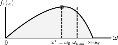
(a) ${\omega}_{0}\leq{\omega}_{\text{max}}$

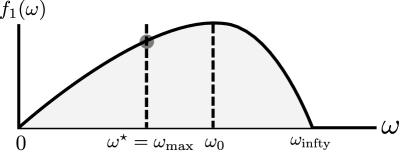
(b) ${\omega}_{0}>{\omega}_{\text{max}}$

Figure 3: Possible situations of ${\omega}_{0}$ with respect to ${\omega}_{\text{max}}$, considering the feasible region of ${\omega}$. The dark circle indicates the position of the optimum point.

V-D Design of $\mathbf{z}$

The optimal design of $\mathbf{z}$ is given in (IV-C) as a closed form expression. Note that the solution of $\mathbf{z}$ is dependent on the choice of other optimization variables. However, as the proposed designs for the other optimization variables do not depend on $\mathbf{z}$, there is no need for further alternation among the design parameters. The Algorithm 2 defines the required steps.

1:$P_{\text{s}}\leftarrow P_{\text{s,max}}$

2:$\mathbf{w}_{\text{tx}}\leftarrow\text{ calculate Tx filter, see (\ref{eq_ch_norm_W2_solution})}$

3:$\mathbf{w}_{\text{rx}}\leftarrow\text{ calculate Rx filter, see (\ref{eq_ch_norm_W_rx_solution})}$

4:$\omega\leftarrow\text{adjust amplification intensity, see Subsection~{}\ref{Chnormratio_design_omega}}$

5:$\mathbf{z}\leftarrow\text{ see (\ref{eq_GP_z})}$

6: return $\left(\mathbf{z},\;\mathbf{W}=\omega\mathbf{w}_{\text{tx}}\mathbf{w}_{\text{rx}}^{H}\right)$

Algorithm 2 Distortion Aware Multi-Stage Rank-1 Relay amplification (MuStR1) for SDNR maximization. The solution is obtained with no alternation among the optimization variables.

V-E Alternating enhancement of MuStR1 (AltMuStR1)

The proposed MuStR1 design is accomplished with no alternation among the optimization variables, see Algorithm 2. In this part we provide an alternating enhancement of MuStR1 which results in an increased performance, at the expense of a higher computational complexity. In order to accomplish this purpose, similar to (19) and (21) we focus on the signal and power values at the destination, after the application of $\mathbf{z}$. In this respect, the values of $\mathbf{w}_{\text{tx}},\mathbf{w}_{\text{rx}},\mathbf{z}$ and $\omega$ will be calculated as a joint alternating optimization. This is done by replacing $\mathbf{H}_{\text{rd}}$ with $\mathbf{z}^{H}\mathbf{H}_{\text{rd}}$ in the design of $\mathbf{w}_{\text{tx}}$, and $\mathbf{d}^{T}$ with $\left(\mathbf{z}^{T}\otimes\mathbf{z}^{H}\right)$ in (43)-(46). The steps $2$-$6$ in Algorithm 2 are then repeated until a stable point is achieved, or a maximum number of iterations is expired. The performance of the proposed (Alt)MuStR1 algorithms in terms of the resulting communication rate, convergence, and computational complexity are studied via numerical simulations in Subsection VII-A. In particular, it is observed that the performance of the AltMuStR1 algorithm reaches close to the performance of GP, with a significantly lower computational complexity.

V-F Convergence

Due to the proposed SDNR approximation, as well as the sub-optimal solutions for $\mathbf{w}_{\text{tx}},\mathbf{w}_{\text{tx}}$ at each iteration, the convergence of the AltMuStR1 algorithm is not theoretically guaranteed. However, it is observed via numerical simulations in SubsectionVII-A, that the algorithm shows a fast average convergence, with a close performance to the proposed GP method for a wide range of system parameters.

V-G Computational complexity

In this part we study the computational complexity associated with AltMuStR1, following simular arguments as given in Subsection IV-E.

V-G1 Algorithm complexity

The calculation of $\mathbf{w}_{\text{rx}}$ is dominated by the expressions (V-B), (40). Exploiting the rank-1 structure of the matrix $\mathbf{h}_{\text{sr}}\mathbf{h}_{\text{sr}}^{H}$ incurring $\mathcal{O}\left(M_{\text{r}}^{3}+2M_{\text{r}}^{2}M_{\text{t}}\right)$ FLOPs. Similarly, the calculation of $\mathbf{w}_{\text{tx}}$ is dominated by (37), resulting in $\mathcal{O}\left(11M_{\text{t}}^{3}/3+2M_{\text{t}}^{2}M_{\text{r}}+2M_{\text{t}}^{2}M_{\text{d}}\right)$ FLOPs. Together with the calculation of $\mathbf{z}$ this requires in total

$$\mathcal{O}\Big{(}\gamma_{3}\left(M_{\text{r}}^{3}+11M_{\text{t}}^{3}/3+2M_{\text{r}}^{2}M_{\text{t}}+2M_{\text{t}}^{2}M_{\text{r}}+2M_{\text{t}}^{2}M_{\text{d}}+M_{\text{d}}^{3}\right)\Big{)}$$ (51)

FLOPs, where $\gamma_{3}$ is the number of the AltMuStR1 algorithm iterations.

V-G2 Processing complexity

Since $\mathbf{W}$ follows a general rank-1 structure, the amplification is simplified to only $M_{\text{t}}+M_{\text{r}}+1$ complex multiplications, and $M_{\text{r}}-1$ summations, totaling $M_{\text{t}}+2M_{\text{r}}$ FLOPs.

VI Comparison with Decode-and-Forward Relaying Under Residual Self-Interference

In the previous sections we studied the behavior of an AF-FD relay under residual self-interference, from the aspects of performance analysis and design methodologies. While an AF relaying is known to provide a simple strategy, it particularly suffers from the aforementioned distortion loop especially when the residual interference power is not ignorable, see Subsection II-D. In this part, we provide a similar study for a setup where the relay operates with DF protocol, in order to act as a comparison benchmark. In a DF relay, the discussed distortion loop is significantly alleviated as the decoding process eliminates the inter-dependency of the received residual interference intensity to the relay transmit signal power, see [16, Section V] for a similar discussion regarding single antenna relays. Note that optimization strategies for FD relays with DF process have been discussed in the literature, see [11, 10, 12, 14], for different relaying setups and assumptions. In order to adopt the available literature to our setup, we follow a modified version of the approach given in [12, 14], where an SDNR maximization problem is studied at a MIMO DF relay. Note that the proposed design in [12, 14] considers a maximization of the SDNR at the relay input/output, taking advantage of spatial and temporal filters. In our system, we focus on the resulting performance from the source to the destination, after the application of the receive filter $\mathbf{z}$, and hence including $P_{\text{s}}$ and $\mathbf{z}$ as optimization variables. Afterwards, similar to [14], we propose a joint optimization where in each step one of the variables is updated to the optimality. A detailed model update and design strategy is given in the following.

VI-A DF Relaying

We define $\mathbf{v}_{\text{in}}\in\mathbb{C}^{M_{\text{r}}}$ as linear filter at the relay input, $\hat{s}_{\text{r}}\in\mathbb{C}$, $\mathbb{E}\{|\hat{s}_{\text{r}}|^{2}\}=1$ as the decoded symbol, and $\mathbf{v}_{\text{out}}\in\mathbb{C}^{M_{\text{t}}}$ as the beamforming vector to transmit the decoded data symbol, see Fig. 5. The end-to-end rate maximization can be equivalently formulated as

$$\underset{\mathbf{v}_{\text{in}},\mathbf{z},\mathbf{Q}\in\mathcal{H},P_{\text{s}}}{\text{max}}\;\; \text{min}\left(\zeta_{\text{sr}},\zeta_{\text{rd}}\right),\;\;$$ (52a)

s.t. $$\text{tr}\left(\mathbf{Q}\right)\leq\tilde{P}_{\text{r,max}},\;P_{\rm{s}}\leq P_{\text{s,max}},\;\text{rank}(\mathbf{Q})=1,$$ (52b)

where the rank-one constraint is imposed to ensure the structure $\mathbf{Q}:=\mathbb{E}\{\mathbf{u}_{{\rm out}}\mathbf{u}_{{\rm out}}^{{H}}\}=\mathbf{v}_{\rm out}\mathbf{v}_{\rm out}^{H}$. The values $\zeta_{\text{sr}}$ and $\zeta_{\text{rd}}$, respectively represent the resulting SDNR in source-to-relay and relay-to destination links which can be calculated as

$$\zeta_{\text{sr}} \approx\frac{P_{\text{s}}\mathbf{v}_{\text{in}}^{H}\mathbf{h}_{{\rm sr}}\mathbf{h}_{{\rm sr}}^{H}\mathbf{v}_{\text{in}}}{\mathbf{v}_{\text{in}}^{H}\Big{(}\sigma_{\text{nr}}^{2}\mathbf{I}_{M_{\text{r}}}+\kappa\mathbf{H}_{\text{rr}}\text{diag}(\mathbf{Q})\mathbf{H}_{\text{rr}}^{H}+\beta\text{diag}\left(\mathbf{H}_{\text{rr}}\mathbf{Q}\mathbf{H}_{\text{rr}}^{H}\right)\Big{)}\mathbf{v}_{\text{in}}},$$ (53)

$$\zeta_{\text{rd}} =\frac{\mathbf{z}^{H}\mathbf{H}_{\text{rd}}\mathbf{Q}\mathbf{H}_{\text{rd}}^{H}\mathbf{z}}{\mathbf{z}^{H}\Big{(}\sigma_{\text{nd}}^{2}\mathbf{I}_{M_{\text{d}}}+\kappa\mathbf{H}_{\text{rd}}\text{diag}(\mathbf{Q})\mathbf{H}_{\text{rd}}^{H}+P_{\text{s}}\mathbf{h}_{\text{sd}}\mathbf{h}_{\text{sd}}^{H}\Big{)}\mathbf{z}}.$$ (54)

where the approximation in (53) follows considering the fact that the self-interference signal constitutes the dominant part of the power in $\mathbf{u}_{{\rm in}}$, and can be regarded as the only cause of distortion signals at the relay, see also (9). Note that (52) is not a convex optimization problem, and also can not be solved in a closed form. Nevertheless, recognizing the generalized Rayleigh quotient structure in (53), (54) we obtain

$$\mathbf{z}^{\star} =\Big{(}\sigma_{\text{nd}}^{2}\mathbf{I}_{M_{\text{d}}}+\kappa\mathbf{H}_{\text{rd}}\text{diag}(\mathbf{Q})\mathbf{H}_{\text{rd}}^{H}+P_{\text{s}}\mathbf{h}_{\text{sd}}\mathbf{h}_{\text{sd}}^{H}\Big{)}^{-1}\mathbf{H}_{\text{rd}}\mathbf{v}_{\text{out}},$$ (55)

$$\mathbf{v}_{\text{in}}^{\star} =\Big{(}\sigma_{\text{nr}}^{2}\mathbf{I}_{M_{\text{r}}}+\kappa\mathbf{H}_{\text{rr}}\text{diag}(\mathbf{Q})\mathbf{H}_{\text{rr}}^{H}+\beta\text{diag}\left(\mathbf{H}_{\text{rr}}\mathbf{Q}\mathbf{H}_{\text{rr}}^{H}\right)\Big{)}^{-1}$$

$$\;\;\;\;\;\;\;\;\;\;\times\mathbf{h}_{\text{sr}}\sqrt{P_{\text{s}}},$$ (56)

where $\mathbf{z}^{\star}$, $\mathbf{v}_{\text{in}}^{\star}$ represent the optimum $\mathbf{z}$, $\mathbf{v}_{\text{in}}$ for a fixed $\mathbf{Q}$ and $P_{\text{s}}$. In order to obtain the optimal $\mathbf{Q},P_{\text{s}}$, the problem in (52) can be re-formulated as

$$\underset{P_{\text{s}},\zeta\in^{+},\mathbf{Q}\in\mathcal{H}}{\text{max}}\;\; \zeta$$ (57a)

s.t. $$\zeta\leq\zeta_{\text{sr}},\;\zeta\leq\zeta_{\text{rd}},$$ (57b)

$$\mathbf{Q}\in\mathcal{H},\;\text{tr}\left(\mathbf{Q}\right)\leq\tilde{P}_{\rm{r,max}},\;\text{rank}(\mathbf{Q})=1,$$ (57c)

where the values of $\mathbf{v}_{\text{in}}$ and $\mathbf{z}$ are fixed. By temporarily relaxing the rank constraint, the above problem can be written as a convex feasibility check over $\mathbf{Q},P_{\text{s}}$, for each value of $\zeta$ as

find $$\mathbf{Q},P_{\text{s}}$$ (58a)

s.t. $$\text{tr}\left(\mathbf{Q}\right)\leq\tilde{P}_{\text{r,max}},\;\;P_{\text{s}}\geq 0,\;\mathbf{Q}\in\mathcal{H},$$ (58b)

$$\text{tr}\left({\mathbf{\Psi}}_{\text{sr}}+{\mathbf{\Phi}}_{\text{sr}}\mathbf{Q}\right)\geq 0,\;\text{tr}\left({\mathbf{\Psi}}_{\text{rd}}+{\mathbf{\Phi}}_{\text{rd}}\mathbf{Q}\right)\geq 0,$$ (58c)

where

$${\mathbf{\Psi}}_{\text{rd}} :=-\zeta\mathbf{z}\mathbf{z}^{H}\left(\sigma_{\text{nd}}^{2}\mathbf{I}_{M_{\text{d}}}+{P}_{\text{s}}\mathbf{h}_{{\text{sd}}}\mathbf{h}_{{\text{sd}}}^{H}\right)$$ (59)

$${\mathbf{\Psi}}_{\text{sr}} :=\mathbf{v}_{\text{in}}\mathbf{v}_{\text{in}}^{H}\left({P}_{\text{s}}\mathbf{h}_{{\text{sr}}}\mathbf{h}_{{\text{sr}}}^{H}-\zeta\sigma_{\text{nr}}^{2}\mathbf{I}_{M_{\text{r}}}\right),$$ (60)

$${\mathbf{\Phi}}_{\text{rd}} :=\mathbf{H}_{{\text{rd}}}^{H}\mathbf{z}\mathbf{z}^{H}\mathbf{H}_{{\text{rd}}}-\zeta\kappa\text{diag}\left(\mathbf{H}_{{\text{rd}}}^{H}\mathbf{z}\mathbf{z}^{H}\mathbf{H}_{{\text{rd}}}\right),$$ (61)

$${\mathbf{\Phi}}_{\text{sr}} :=-\zeta\left(\kappa\text{diag}\left(\mathbf{H}_{{\text{rr}}}^{H}\mathbf{v}_{\text{in}}\mathbf{v}_{\text{in}}^{H}\mathbf{H}_{{\text{rr}}}\right)+\beta\mathbf{H}_{{\text{rr}}}^{H}\text{diag}\left(\mathbf{v}_{\text{in}}\mathbf{v}_{\text{in}}^{H}\right)\mathbf{H}_{{\text{rr}}}\right).$$ (62)

Note that the iterations of the defined feasibility check will be continued, following a bi-section search procedure until an optimum $\zeta$ is obtained with sufficient accuracy. Fortunately, for the special structure of (58) as a complex-valued semi-definite program with three linear constraints, we can always achieve an optimal rank-$1$ $\mathbf{Q}\in\mathcal{H}$, following [57, Theorem 3.2]. The optimal $\mathbf{v}_{\text{in}}$ is hence obtained as

$$\mathbf{v}_{\text{out}}^{\star}={\mathbf{Q}^{\star}}^{\frac{1}{2}},$$ (63)

where $\mathbf{Q}^{\star}$ represents the obtained $\mathbf{Q}$ for the highest feasible $\zeta$.

VI-A1 Algorithm initialization

The initial value of $\mathbf{Q}$ is obtained by setting $\mathbf{v}_{\text{out}}$ as the dominant eigenvector of $\mathbf{H}_{\text{rd}}$, resulting in a maximum-ratio transmission, and assuming a maximum transmit power at the relay. The initial values of $\mathbf{v}_{\text{in}},\mathbf{z}$ are then obtained from (55) and (56). Moreover, the feasible values of $\zeta$ is necessarily located in the region $[0,\zeta_{\text{max}}]$ where

$$\zeta_{\text{max}}:=\text{min}\left\{\frac{{P}_{\text{s,max}}\|\mathbf{h}_{{\rm sr}}\|_{2}^{2}}{\sigma_{\text{nr}}^{2}},\frac{{P}_{\text{r,max}}\lambda_{\text{max}}\left\{\mathbf{H}_{{\text{rd}}}\mathbf{H}_{{\text{rd}}}^{H}\right\}}{\sigma_{\text{nd}}^{2}}\right\}$$ (64)

corresponds to the minimum of the individual link qualities, assuming $\beta=\kappa=0$, and will be used as the initial bounds for the aforementioned bi-section search.

VI-A2 Convergence and optimality gap

The solutions in (55)-(63), result in a necessary improvement of $\zeta$, since in each step the defined sub-problem is solved to optimality. Moreover, since the performance of the studied relay system is bounded from above, see (64), the defined iterative update results in a necessary convergence. However, the global optimality of the obtained solution may not be guaranteed, since the problem is not a jointly convex optimization problem. Hence, the resulting solution depends on the used initialization. On order to observe this, we have repeated Algorithm 3 with several random initializations in Fig. 4, in comparison to the initialization defined in Subsection VI-A1. It is observed that the proposed initialization in Algorithm 3 reaches close to the best achievable performance via several initializations. Hence, it is used as the performance benchmark for an achievable SDNR in an FD-DF relaying system.

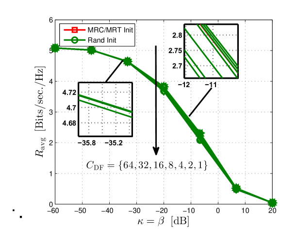
Figure 4: Evaluation of the DF relaying performance with multiple random initializations, compared to the used MRC/MRT initialization. $C$

1:$P_{\rm s}\leftarrow P_{\text{s,max}}\times 10^{-2}$

2:$\text{counter}_{1}\leftarrow 0$

3:repeat  (main optimization steps)

4:    $\text{counter}_{1}\leftarrow\text{counter}_{1}+1$

5:    $\mathbf{v}_{\text{in}}\leftarrow\mathbf{v}_{\text{in}}^{\star},\;\;\text{see~{}(\ref{eq_DF_v_in_star})}$

6:    $\mathbf{z}\leftarrow\mathbf{z}^{\star},\;\;\text{see~{}(\ref{eq_DF_z_star})}$

7:    $\text{counter}_{2}\leftarrow 0$

8:    $\zeta_{\text{min}}\leftarrow 0$

9:    $\zeta_{\text{max}}\leftarrow\text{see~{}(\ref{eq_DF_zeta_max})}$

10:    repeat  (bi-section search steps)

11:         $\zeta\leftarrow(\zeta_{\text{min}}+\zeta_{\text{max}})/2$

12:         if (58a)-(58b) is feasible then

13:             $\zeta_{\text{min}}\leftarrow\zeta$

14:         else

15:             $\zeta_{\text{max}}\leftarrow\zeta$

16:         end if

17:    until $\text{counter}_{2}\leq C_{2}$

18:    $\zeta^{\text{counter}_{1}}\leftarrow(\zeta_{\text{min}}+\zeta_{\text{max}})/2$

19:    $P_{\text{s}}\leftarrow P_{\text{s}}^{\star},\;\;\text{see~{}(\ref{eq_DF_opt_Ps_Q})}$

20:    $\mathbf{v}_{\text{out}}\leftarrow\mathbf{v}_{\text{out}}^{\star},\;\;\text{see~{}(\ref{eq_DF_v_out})}$

21:until $\text{counter}_{1}\leq C_{\text{DF}}\;\;\text{or}\;\;\zeta^{\text{counter}_{1}}-\zeta^{\text{counter}_{1}-1}\leq{c}_{1}$

22:return $\left(P_{\text{s}},\mathbf{z},\mathbf{v}_{\text{in}},\mathbf{v}_{\text{our}},\right)$

Algorithm 3 An iterative rate maximization algorithm for decode-and-forward relaying. $C_{\text{DF}},C_{2}\in\mathbb{N}$ respectively represent the number of the main optimization steps and the bi-section process, and ${c}_{1}\in^{+}$ determines the stability condition.

Figure 5: A schematic of a decode-and-forward relaying process. $\rho\{\cdot\}$ and $\hat{s}_{\text{r}}$ represent the decoding process, and the estimate of the transmitted symbol, $s$, at the relay. The receive and transmit spatial filters are represented as $\mathbf{v}_{\text{in}}$ and $\mathbf{v}_{\text{out}}$, respectively. The bold arrows represent the vector signals while the dashed arrows represent the scalars.

VII Simulation Results

TABLE II: Default setup parameters

Parameter	$P_{\text{max}}:=P_{\text{s,max}}=P_{\text{r,max}}$	$\sigma_{\text{n}}^{2}:=\sigma_{\text{nr}}^{2}=\sigma_{\text{nd}}^{2}$	$\kappa=\beta$	$M:=M_{\text{t}}=M_{\text{r}}=M_{\text{d}}$	$\rho_{\text{rr}}$	$\rho_{\text{sr}}=\rho_{\text{rd}}$	$\rho_{\text{sd}}$	$K_{R}$
Value	$1~{}[Watt]$	$-40~{}\text{[dBW]}$	$-40~{}\text{[dB]}$	$4$	$1$	$-30~{}\text{[dB]}$	$-60~{}\text{[dB]}$	$10$

In this section we evaluate the behavior of the studied FD AF relaying setup via numerical simulations. In particular, we evaluate the proposed GP design in Section IV, as well as the (Alt)MuStR1 algorithms in Section V, under the impact of hardware inaccuracies, in comparison with the available relevant methods in the literature. We assume that $\mathbf{h}_{\text{sr}},\mathbf{H}_{\text{rd}}$ and $\mathbf{h}_{\text{sd}}$ follow an uncorrelated Rayleigh flat-fading model, where $\rho_{\text{sr}},\,\rho_{\text{rd}}$ and $\rho_{\text{sd}}\in^{+}$ represent the path loss. For the self-interference channel, we follow the characterization reported in [21]. In this respect we have $\mathbf{H}_{\text{rr}}\sim\mathcal{CN}\left(\sqrt{\frac{\rho_{\text{rr}}K_{R}}{1+K_{R}}}\mathbf{H}_{0},\frac{1}{1+K_{R}}\mathbf{I}_{M_{\text{t}}}\otimes\mathbf{I}_{M_{\text{r}}}\right)$ where $\rho_{\text{rr}}$ represents the self-interference channel strength, $\mathbf{H}_{0}$ is a deterministic term and $K_{R}$ is the Rician coefficient. For each channel realization the resulting performance in terms of the communication rate, i.e., $\log_{2}(1+\text{SDNR})$, is evaluated by employing different design strategies and for various system parameters. The overall system performance in terms of the average rate, i.e., $R_{\text{avg}}$, is then evaluated via Monte-Carlo simulations by employing $500$ channel realizations. Unless explicitly stated, the defined parameters in Table II are used as our default setup.

VII-A Algorithm analysis

In this subsection we study the behavior of the proposed iterative algorithms, i.e., GP and (Alt)MuStR1, in terms of the convergence speed, approximation accuracy, and computational complexity. Moreover, we study the gap of the proposed GP method with the optimality, with the help of an extensive numerical simulation.

VII-A1 Convergence

Both GP and AltMuStR1 operate based on iterative update of the variables, until a stable point is obtained. A study on the convergence behavior of these algorithms are necessary, in order to verify the algorithm function, and also as a measure of the required computational effort.

In Fig. 6 (a) the average convergence behavior of the GP algorithm is depicted. At each iteration, the obtained performance is depicted as a percentage of the final performance after convergence, where $\text{SDNR}^{\star}$ is the SDNR at the convergence. It is observed that the convergence speed differs, for different values of transceiver inaccuracy. This is expected, as a higher distortion results in the complication of the mathematical structure by signifying non-quadratic terms, see (17), and requires the application of the projection procedure (Subsection IV-A1) more often. It is observed from our simulations that the algorithm requires $10^{2}$ to $10^{4}$ number of iterations to converge, depending on the value of the distortion coefficients $\kappa,\beta$.

In Fig. 6 (b) the average convergence behavior of the proposed AltMuStR1 is depicted. Note that unlike GP, AltMuStR1 operates based on the local increase of SDNR in the defined relaying segments, see Section V. Hence, a theoretical guarantee on the monotonic increase of the overall SDNR in each iteration is not available. Nevertheless, the numerical evaluation shows that the algorithm converges within much fewer number of iterations, with an effective increase in each step. Similar to GP, a higher value of $\kappa,\beta$ results in a slower convergence.

VII-A2 Computational complexity

Other than the required number of iterations, the computational demand of an algorithm is impacted by the required per-iteration complexity. In Fig. 6 (c), the required CPU time of the proposed algorithms are depicted as the number of antennas increase. The reported CPU time is obtained using an Intel Core i$5-3320$M processor with the clock rate of $2.6$ GHz and $8$ GB of random-access memory (RAM). As our software platform we have used MATLAB $2013$a, on a $64$-bit operating system. While the GP method is considered as the performance benchmark, the proposed (Alt)MuStR1 algorithms show a significant advantage to the GP algorithm in terms of computational complexity.

VII-A3 Approximation accuracy

The proposed (Alt)MuStR1 algorithms are based on the used approximation (46) and (47). In this regard, the choice of the approximation order $K$ leads to a trade-off between algorithm complexity and the resulting performance. In Fig. 6-(d) the exact, and approximated SDNR values are depicted for a pessimistic case of $\kappa=0.1$. By repeating such experiments, we have decided on $K=5$ as a good balance between approximation accuracy and the resulting complexity.

VII-A4 GP optimality gap

Via the application of the gradient ascend the proposed GP converges with a monotonically increasing objective. Nevertheless, the global optimality of the resulting stationary point may not be guaranteed, due to the possibility of a local extrema. In Fig. 6 (e) the performance of GP algorithm is evaluated with multiple random initializations, where the best converging point is considered as the algorithm solution. It is observed that the occurrence of the non-optimum solutions is more likely for higher values of $\kappa,\beta$, as a larger number of initial points results in a better performance. Nevertheless, it is observed that no significant performance improvement is observed by employing more than $C_{1}=10$ number of random initial points. We consider the obtained performance of the GP algorithm with $C_{1}=10$ as our performance benchmark for FD AF relaying hereinafter.

VII-A5 Rank profile

In the proposed (Alt)MuStR1 method, a rank-1 relay amplification is assumed. Hence, it is interesting to observe how the solution to the GP method behaves in terms of the matrix rank. In Fig. 6 (f) the energy distribution of the singular values of the obtained relay amplification from the GP method is depicted. It is observed that for most of the distortion conditions, the highest singular value holds almost all of the energy, indicating an approximately rank-1 property.

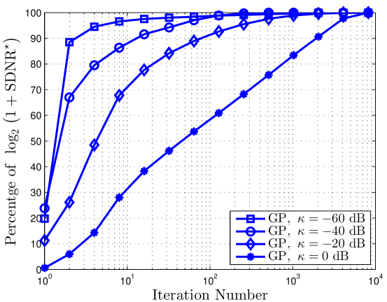
(a) Convergence-GP

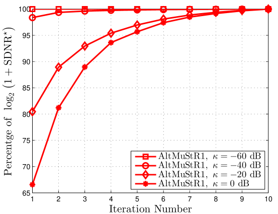
(b) Convergence-AltMuStR1

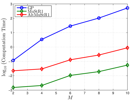
(c) CPU Time

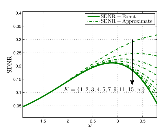
(d) SDNR Approximation

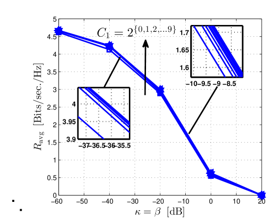
(e) GP-Initialization

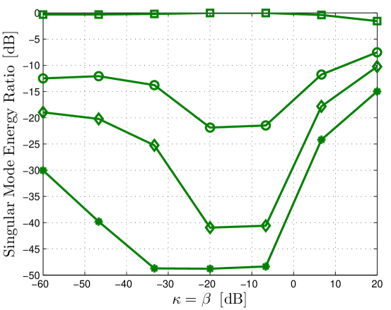
(f) Singular energy distribution

Figure 6: Numerical algorithm analysis, including the average convergence behavior of the proposed GP algorithm (a), the AltMuStR1 algorithm (b), a comparison on computational complexity (c), accuracy of the SDNR approximation (d), impact of algorithm initialization on the GP method (e), and the singular mode energy profile for the obtained $\mathbf{W}$ from the GP method (f).

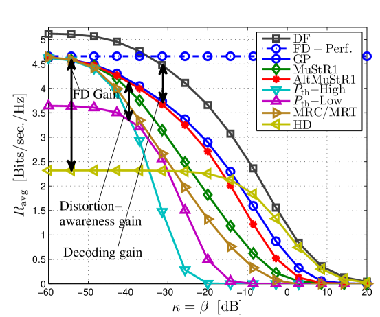
(a) $R_{\text{avg}}$ vs. Distortion

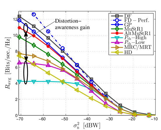
(b) $R_{\text{avg}}$ vs. Noise

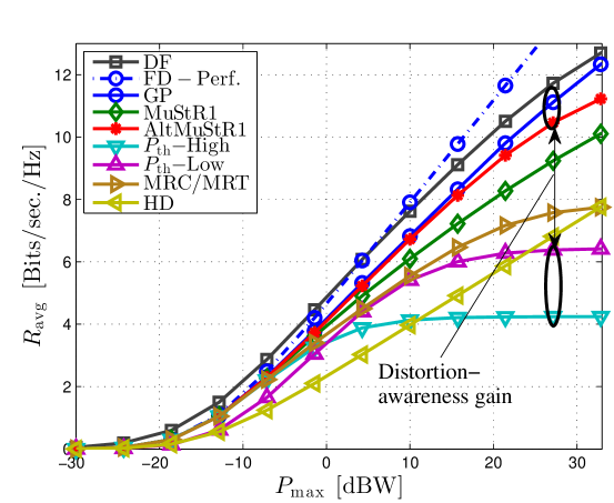
(c) $R_{\text{avg}}$ vs. Max. Tx power

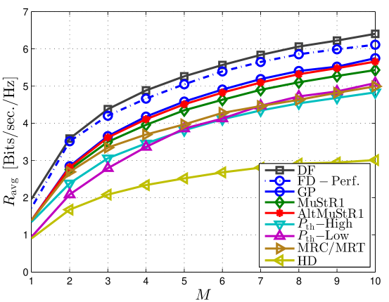
(d) $R_{\text{avg}}$ vs. $M$

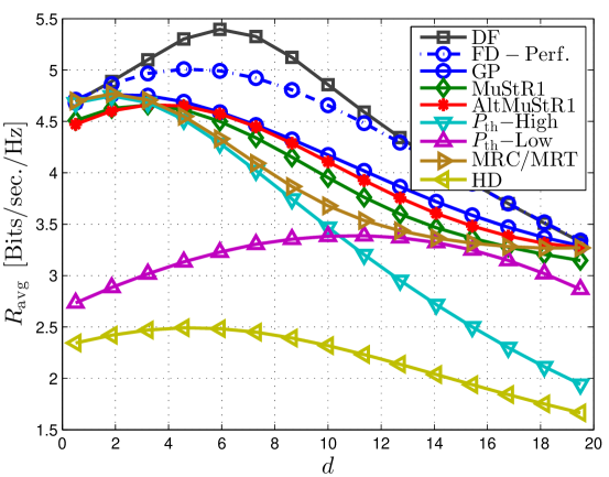
(e) $R_{\text{avg}}$ vs. Relay position

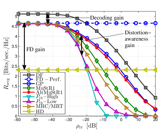
(f) $R_{\text{avg}}$ vs. $\rho_{\text{rr}}$

Figure 7: The comparison of average system performance $R_{\text{avg}}$ under different parameter ranges.

VII-B Performance comparison

In this part we evaluate the performance of the proposed designs, in comparison with the available designs in the literature.

VII-B1 Available design approaches

We divide the relevant available literature on the FD AF relaying design into three main approaches. Firstly, as considered in [22, 23], the SIC is purely relegated to the relay receiver end, via a combined time domain analog/digital cancellation techniques. The aforementioned approach imposes no design constraint on the self-interference power, i.e., $P_{\text{intf}}\leq\infty$, where $P_{\text{intf}}$ represents the self-interference power prior to analog/digital cancellation. Secondly, the SIC is purely done via transmit beamforming at the null space of the relay receive antennas, e.g., [25, 26, 27, 28, 29, 30], hence imposing a zero interference power constraint for transmit beamforming design, i.e., $P_{\text{intf}}\leq 0$. Finally, as a generalization of the aforementioned extreme approaches, a combined transmit beamforming and analog/digital cancellation at the receiver is considered in [33, 34]. In the aforementioned case it is assumed that the received self-interference power should not exceed a certain threshold ($P_{\text{th}}$), i.e., $P_{\text{intf}}\leq P_{\text{th}}$. In all of the aforementioned cases, due to the perfect hardware assumptions, and upon imposition of the required self-interference power constraint, the SIC is assumed to be perfect. In our simulations, we evaluate the generalized approach in [34, 33] by once assuming a high self-interference power threshold, i.e., $P_{\text{th}}=P_{\text{r,max}}$, denoted as ’$P_{\text{th}}$-High’, and once assuming a low self-interference power threshold, i.e., $P_{\text{th}}=0.01\times P_{\text{r,max}}$, denoted as ’$P_{\text{th}}$-Low’. Moreover, the proposed approach in [38] is evaluated as a sub-optimal solution, where a power adjustment method is done at the relay, assuming a maximum ratio combining/transmission (MRC/MRT). The performance of an FD-AF relay with perfect hardware, i.e., $\kappa=0$, is also illustrated as ’FD-Perf.’.

VII-B2 Decoding gain

Other than the defined approaches for FD AF relaying, it is interesting to evaluate the impact of decoding in the studied system. This is since in a DF relay, the discussed distortion loop is significantly alleviated as the decoding process eliminates the inter-dependency of the received residual interference intensity to the relay transmit power. See Section VI for the detailed implementation and performance evaluation of the DF process.

VII-B3 Numerical results

In Figs. 7 (a)-(f) the average communication rate is evaluated under various system parameters.

In Fig. 7 (a) the impact of the transceiver inaccuracy is depicted. It is observed that as $\kappa=\beta$ increase, the communication performance decreases for all methods. In this respect, the HD setup remains more robust against the hardware distortions, and outperforms the FD setup for large values of $\kappa=\beta$. This is since the strong self-interference channel, as the main cause of distortion, is not present for a HD setup. Relative to the benchmark performance for the FD-AF relaying (GP), a significant decoding gain is observed for the big values of $\kappa$, where the system performance is dominated by the impact of distortion loop, see Subsection II-D. Moreover, it is observed that the proposed AltMuStR1 method performs close to the GP method for different values of $\kappa$. The performance of ’$P_{\text{th}}$-High’ reaches close to optimality for a small $\kappa$, where the ’$P_{\text{th}}$-Low’ reaches a relatively better performance as $\kappa$ increases. Nevertheless, both of the aforementioned methods degrade rapidly for higher values of $\kappa$. This is expected, as the impacts of hardware inaccuracies are not taken into account in the aforementioned approaches.

In Fig. 7 (b) and (c), the opposite impact of the thermal noise variance, $\sigma_{\text{n}}^{2}=\sigma_{\text{nr}}^{2}=\sigma_{\text{nd}}^{2}$, and the maximum transmit power, $P_{\text{max}}=P_{\text{s,max}}=P_{\text{r,max}}$, is observed on the average system performance. This is expected, as an increase (decrease) in $P_{\text{max}}$ ($\sigma_{\text{n}}^{2}$) increases the signal-to-noise ratio, while keeping the signal-to-distortion ratio intact. Furthermore, it is observed that in a low noise (high power) region the performance of the methods with perfect hardware assumptions saturate. This is since the role of hardware distortions become dominant for a high power or a low noise system.

In Fig. 7 (d) the resulting system performance is depicted with respect to the number of antennas. It is observed that the performance of all methods increase as the number of antennas increase. Moreover, the performance of the proposed (Alt)MuStR1 methods remain close to the benchmark GP performance. This is promising, considering the increasing computational complexity of the GP method as the number of antenna increases.

In Fig. 7 (e) the impact of the relay position is observed. In this regard, it is assumed that the source is located with the distance $d_{\text{sr}}$ from the relay where the relay is located with the distance $d_{\text{rd}}=20-d_{\text{sr}}$ from the source. The path loss values for each link is then obtained as $\rho_{X}=\frac{0.1}{d_{X}^{2}}$, $X\in\{\text{sr},\text{rd}\}$. As expected, the decoding gain decreases when the relay is positioned close to the source or destination. Interestingly, the performance of the (Alt)MuStR1 methods are slightly dominated by ’$P_{\text{th}}$-High’, when relay is positioned very close to the source. The reason is that in such a situation the bottleneck shifts to the relay-destination path as the source-relay channel is very strong and is not degraded by the impact of distortion from the self-interference path. Nevertheless, the distortion awareness in (Alt)MuStR1 destructively limits the performance of the relay-destination path in order to avoid distortion on the relay receiver. It is worth mentioning that this mismatch does not appear for the GP method, since the final SDNR is considered as the optimization objective which remains relevant for any relay position.

In Fig. 7 (f) the impact of the self-interference channel intensity is depicted. It is observed that the performance of the FD relay operation, for all design methods, degrades as the $\rho_{\text{rr}}$ increase while the performance of the HD method is not changed. As expected, the performance of the methods with perfect hardware assumptions degrades faster compared to the proposed methods. Moreover, the performance of the proposed AltMuStR1 method remains close to that of GP, for different values of the self-interference channel intensity. It is observed that the MRC/MRT method suffers from a rapid degradation, when $\kappa$ or $\rho_{\text{rr}}$ increases, also see Fig. 7 (a). This is expected, since the transmit/receive filters are designed with no consideration of the impact of distortion, e.g., the instantaneous CSI regarding the self-interference channel is not effectively used to control the impact of distortion.

In Fig. 9 the impact of the accuracy of transmit and receiver chains are studied, where $\kappa\text{[dB]}+\beta\text{[dB]}=\mathcal{A}_{\text{sum}}$, i.e., the sum-accuracy (in dB scale) is fixed. For instance, for an FD transceiver with massive antenna arrays where the utilization of analog cancelers is not feasible, and also the quantization bits are considered as costly resources, the value of $A_{\text{sum}}$ is related to the total number of quantization bits. The similar evaluation regarding the number of transmit/receive antennas is performed in Fig. 8, where $M_{\text{t}}+M_{\text{r}}=\mathcal{M}_{\text{sum}}$. It is observed that different available resources, i.e., $\mathcal{A}_{\text{sum}}$, $\mathcal{M}_{\text{sum}}$, result in different optimal allocations. However, as a general insight, it is observed that the performance is degraded when resources are concentrated only on transmit or receive side. Please note that similar approach can be used for evaluating different cost models for accuracy and antenna elements, relating different system setups, or SIC specifications.

In Table III a compact comparison is made between the studied relaying strategies in terms of the algorithm computational complexity, processing complexity, as well as the resulting performance under different impairment conditions ($\kappa=\beta$). The percentage values indicate the performance improvement in the scale of the optimal FD-AF performance, compared to three common relaying schemes. This includes the HD-AF relaying, the FD-DF relaying, as well as the FD-AF relaying with simplified modeling, i.e., the best choice among ’$P_{\text{th}}$-High’ and ’$P_{\text{th}}$-Low’ schemes. As expected, the gain of a design with consideration of the distortion is invaluable for a large $\kappa$, and can be achieved with a reasonable computational complexity, via the utilization of the AltMuStR1 algorithm.

TABLE III: Complexity-performance tradeoff for different relaying strategies.

Alg.	Complexity (alg.)	Complexity (proc.)	$\kappa=-60$ dB	$\kappa=-30$ dB	$\kappa=-10$dB	Compared to
GP	$\mathcal{O}\left(16/3(\gamma_{1}+\gamma_{2})M^{6}\right)$	$2M^{2}-M$	-10% +49% 0.1 %	-19% +38% +31 %	-48% -15% +99 %	FD-DF HD-AF FD-Simple
AltMuStR1	$\mathcal{O}\left((\gamma_{3}35/3)M^{3}\right)$	$3M$	-10% +49% 0.1 %	-21% +36% +29 %	-79% -38% +76 %	FD-DF HD-AF FD-Simple

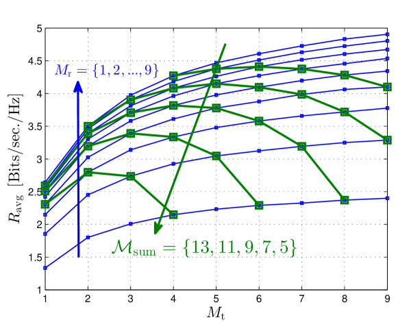
Figure 8: Impact of the number of antennas, $M_{\text{t}}+M_{\text{r}}=\mathcal{M}_{\text{sum}}$. $M_{\text{d}}=1$.

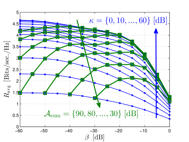
Figure 9: Impact of the transmit/receive chain accuracy, $\kappa+\beta=\mathcal{A}_{\text{sum}}$.

VIII Conclusion

The impact of hardware inaccuracies is of particular importance for an FD transceiver, due to the high strength of the self-interference channel. In particular, for an FD-AF relaying system, such impact is significant due to the inter-dependency of the relay transmit power, as well as the residual self-interference, which results in a distortion loop effect. In this work, we have analytically observed the aforementioned effect, and proposed optimization strategies to alleviate the resulting degradation. It is observed that the proposed GP algorithm can be considered as the performance benchmark, though, imposing a high computational complexity. On the other hand, the proposed (Alt)MuStR1 methods provide a significant reduction in the complexity, at the expense of a slightly lower performance. In particular, the comparison to the available schemes in the literature reveals that for a system with a small thermal noise variance, or a high power or transceiver inaccuracy, the application of a distortion-aware design is essential. Moreover, it is observed that an FD-DF relay is more robust against the increase of hardware distortions, compared to an FD-AF relay. This is expected, since the observed distortion loop for FD AF relays does not exist for an FD-DF relay, due to decoding.

Appendix A Optimal $P_{\text{s}}$ as a function of $\mathbf{W}$

Let $\mathbf{W}$ and $\mathbf{z}$ be the fixed (given) relay amplification and receive filter, respectively. From (15)-(21), the SDNR at the destination can be written as a function of $P_{\text{s}}$

$$\text{SDNR}(P_{\text{s}})=\frac{\alpha_{1}P_{\text{s}}}{\alpha_{2}P_{\text{s}}+\alpha_{3}},$$ (65)

where $\alpha_{1},\alpha_{2},\alpha_{3}\in^{+}$, such that

$$\alpha_{1} :=\mathbf{z}^{{H}}\mathbf{H}_{{\text{rd}}}\mathbf{W}\mathbf{h}_{{\text{sr}}}\mathbf{h}_{{\text{sr}}}^{{H}}\mathbf{W}^{{H}}\mathbf{H}_{{\text{rd}}}^{{H}}\mathbf{z},$$

$$\alpha_{2} :=\mathbf{q}\left(\mathbf{W},\mathbf{z}\right)\text{vec}\left(\mathbf{h}_{\text{sr}}\mathbf{h}_{\text{sr}}^{H}\right)+\mathbf{z}^{{H}}\mathbf{h}_{\text{sd}}\mathbf{h}_{{\text{sd}}}^{H}\mathbf{z}-\alpha_{1},$$

$$\alpha_{3} :=\mathbf{z}^{{H}}\mathbf{z}\sigma_{\text{nd}}^{2}+\mathbf{q}\left(\mathbf{W},\mathbf{z}\right)\text{vec}\left(\sigma_{\text{nr}}^{2}\mathbf{I}_{M_{\text{r}}}\right),$$

$$\mathbf{q}\left(\mathbf{W},\mathbf{z}\right): =\left(\mathbf{z}^{T}\otimes\mathbf{z}^{H}\right)\left(\mathbf{H}_{\text{rd}}^{*}\otimes\mathbf{H}_{\text{rd}}\right){\mathbf{\Theta}\big{(}\mathbf{W},\mathbf{H}_{\text{rr}},\kappa,\beta\big{)}.}$$ (66)

It is observed, by taking the first and second order derivatives of the obtained function in (65), that SDNR is an increasing and concave function over $P_{\text{s}}$, which concludes the proof.

Appendix B Equivalent Transmit Distortion Channel Expression

Via the application of $\mathbf{w}_{\text{tx}}$, the collective received distortion power due to the relay transmission, here denoted as $\theta_{1}$, is written as

$${\theta_{1}} =P_{\text{r,max}}\kappa\text{tr}\bigg{(}\mathbf{H}_{\text{rr}}\text{diag}\left(\mathbf{w}_{\text{tx}}\mathbf{w}_{\text{tx}}^{H}\right)\mathbf{H}_{\text{rr}}^{H}+\mathbf{H}_{\text{rd}}\text{diag}\left(\mathbf{w}_{\text{tx}}\mathbf{w}_{\text{tx}}^{H}\right)\mathbf{H}_{\text{rd}}^{H}\bigg{)}$$

$$+P_{\text{r,max}}\beta\text{tr}\bigg{(}\text{diag}\left(\mathbf{H}_{\text{rr}}\mathbf{w}_{\text{tx}}\mathbf{w}_{\text{tx}}^{H}\mathbf{H}_{\text{rr}}^{H}\right)\bigg{)}$$

$$=\sum_{i\in\mathbb{F}_{M_{\text{t}}}}\sum_{X\in\{\text{rr,~{}rd}\}}P_{\text{r,max}}\kappa\text{tr}\big{(}\mathbf{H}_{X}\mathbf{\Gamma}_{i}^{M_{\text{t}}}\mathbf{w}_{\text{tx}}\mathbf{w}_{\text{tx}}^{H}{\mathbf{\Gamma}_{i}^{M_{\text{t}}}}^{H}\mathbf{H}_{X}^{H}\big{)}$$

$$+\sum_{i\in\mathbb{F}_{M_{\text{r}}}}P_{\text{r,max}}\beta\text{tr}\big{(}\mathbf{\Gamma}_{i}^{M_{\text{r}}}\mathbf{H}_{\text{rr}}\mathbf{w}_{\text{tx}}\mathbf{w}_{\text{tx}}^{H}\mathbf{H}_{\text{rr}}^{H}{\mathbf{\Gamma}_{i}^{M_{\text{t}}}}^{H}\big{)}$$

$$=\kappa P_{\text{r,max}}\sum_{i\in\mathbb{F}_{M_{\text{t}}}}\sum_{X\in\{\text{rr,~{}rd}\}}\left\|\mathbf{H}_{X}\mathbf{\Gamma}_{i}^{M_{\text{t}}}\mathbf{w}_{\text{tx}}\right\|_{2}^{2}$$

$$+\beta P_{\text{r,max}}\sum_{i\in\mathbb{F}_{M_{\text{t}}}}\left\|\mathbf{\Gamma}_{i}^{M_{\text{r}}}\mathbf{H}_{\text{rr}}\mathbf{w}_{\text{tx}}\right\|_{2}^{2}$$

$$=P_{\text{r,max}}\Bigg{\|}\left[\begin{array}[]{c}\lfloor\sqrt{\kappa}\mathbf{H}_{X}\mathbf{\Gamma}_{i}^{M_{\text{t}}}\mathbf{w}_{\text{tx}}\rfloor_{i\in\mathbb{F}_{M_{\text{t}}},\;X\in\{\text{rr,~{}rd}\}}\\ \lfloor\sqrt{\beta}\mathbf{\Gamma}_{i}^{M_{\text{r}}}\mathbf{H}_{\text{rr}}\mathbf{w}_{\text{tx}}\rfloor_{i\in\mathbb{F}_{M_{\text{r}}}}\end{array}\right]\Bigg{\|}_{2}^{2}$$ (69)

$$=P_{\text{r,max}}\Bigg{\|}\underbrace{\left[\begin{array}[]{c}\lfloor\sqrt{\kappa}\mathbf{H}_{X}\mathbf{\Gamma}_{i}^{M_{\text{t}}}\rfloor_{i\in\mathbb{F}_{M_{\text{t}}},\;X\in\{\text{rr,~{}rd}\}}\\ \lfloor\sqrt{\beta}\mathbf{\Gamma}_{i}^{M_{\text{r}}}\mathbf{H}_{\text{rr}}\rfloor_{i\in\mathbb{F}_{M_{\text{r}}}}\end{array}\right]}_{=:\mathbf{H}_{\text{D,tx}}}\mathbf{w}_{\text{tx}}\Bigg{\|}_{2}^{2},$$ (72)

where $\mathbf{\Gamma}_{i}^{M}$ is an $M\times M$ all-zero matrix, except for the $i$-th diagonal element equal to one, and $\mathbf{H}_{\text{D,tx}}$ is viewed as the equivalent distortion channel.

Appendix C Derivation of (41)-(42) and the coefficients (43)-(47)

The desired signal power at the destination prior to the application of $\mathbf{z}$, here denoted as $\theta_{2}$, can be calculated applying the known matrix equalities [50, Eq. (486), (487), (496)] as

$$\theta_{2} =P_{\text{s}}\text{tr}\left(\mathbf{H}_{\text{rd}}{\mathbf{W}}\mathbf{h}_{\text{sr}}\mathbf{h}_{\text{sr}}^{H}{\mathbf{W}}^{H}\mathbf{H}_{\text{rd}}^{H}\right)$$

$$={\omega}P_{\text{s}}\text{tr}\left(\mathbf{H}_{\text{rd}}\mathbf{w}_{\text{tx}}\mathbf{w}_{\text{rx}}^{H}\mathbf{h}_{\text{sr}}\mathbf{h}_{\text{sr}}^{H}\left(\mathbf{w}_{\text{tx}}\mathbf{w}_{\text{rx}}^{H}\right)^{H}\mathbf{H}_{\text{rd}}^{H}\right)$$

$$={\omega}P_{\text{s}}\mathbf{d}_{M_{\text{t}}}^{T}\Big{(}\left(\mathbf{H}_{\text{rd}}^{*}(\mathbf{w}_{\text{tx}}\mathbf{w}_{\text{rx}}^{H})^{*}\right)\otimes\left(\mathbf{H}_{\text{rd}}\mathbf{w}_{\text{tx}}\mathbf{w}_{\text{rx}}^{H}\right)\Big{)}\text{vec}\left(\mathbf{h}_{\text{sr}}\mathbf{h}_{\text{sr}}^{H}\right)$$

$$={\omega}P_{\text{s}}\mathbf{d}_{M_{\text{t}}}^{T}\left(\mathbf{H}_{\text{rd}}^{*}\otimes\mathbf{H}_{\text{rd}}\right)\tilde{\mathbf{W}}\text{vec}\left(\mathbf{h}_{\text{sr}}\mathbf{h}_{\text{sr}}^{H}\right)$$

$$={\omega}a_{\text{d}},$$ (74)

where $a_{\text{d}}$ and $\mathbf{d}_{M_{\text{t}}}$ are respectively defined in (43) and immediately after (47), and $\tilde{\mathbf{W}}:=(\mathbf{w}_{\text{tx}}\mathbf{w}_{\text{rx}}^{H})^{*}\otimes(\mathbf{w}_{\text{tx}}\mathbf{w}_{\text{rx}}^{H})$. Similarly, following (13)-(16) and the matrix identity [50, Eq. (186)] the noise+interference power at destination, here denoted as $\theta_{3}$, is calculated as

$$\theta_{3} \;\;=N-a_{\text{d}}{\omega}+\text{tr}\left(\mathbf{H}_{\text{rd}}\mathbb{E}\{\mathbf{r}_{{\rm out}}\mathbf{r}_{{\rm out}}^{{H}}\}\mathbf{H}_{\text{rd}}^{H}\right)$$ (75)

$$\;\;=N-a_{\text{d}}{\omega}+\mathbf{d}_{M_{\text{d}}}^{T}\left(\mathbf{H}_{\text{rd}}^{*}\otimes\mathbf{H}_{\text{rd}}\right)\text{vec}\left(\mathbb{E}\{\mathbf{r}_{{\rm out}}\mathbf{r}_{{\rm out}}^{{H}}\}\right)$$

$$\;\;=N-a_{\text{d}}{\omega}+\mathbf{d}_{M_{\text{d}}}^{T}\left(\mathbf{H}_{\text{rd}}^{*}\otimes\mathbf{H}_{\text{rd}}\right)\left(\mathbf{I}_{M_{\text{t}}^{2}}+\kappa\mathbf{S}_{\text{D}}^{M_{\text{t}}}\right)$$

$$\quad\quad\quad\quad\quad\quad\quad\quad\quad\quad\quad\times\Big{(}\mathbf{I}_{M_{\text{t}}^{2}}-{\omega}\tilde{\mathbf{W}}\mathbf{C}\Big{)}^{-1}{\omega}\tilde{\mathbf{W}}\mathbf{c}$$

$$\;\;=N-a_{\text{d}}{\omega}+\mathbf{d}_{M_{\text{d}}}^{T}\left(\mathbf{H}_{\text{rd}}^{*}\otimes\mathbf{H}_{\text{rd}}\right)\left(\mathbf{I}_{M_{\text{t}}^{2}}+\kappa\mathbf{S}_{\text{D}}^{M_{\text{t}}}\right)$$

$$\quad\quad\quad\quad\quad\quad\quad\quad\quad\quad\quad\times\sum_{k\in\{0\cdots\infty\}}\left({\omega}\tilde{\mathbf{W}}\mathbf{C}\right)^{k}{\omega}\tilde{\mathbf{W}}\mathbf{c}$$ (76)

$$\;\;\approx N-a_{\text{d}}{\omega}+\sum_{k\in\mathbb{F}_{K}}\mathbf{d}_{M_{\text{d}}}^{T}\left(\mathbf{H}_{\text{rd}}^{*}\otimes\mathbf{H}_{\text{rd}}\right)\left(\mathbf{I}_{M_{\text{t}}^{2}}+\kappa\mathbf{S}_{\text{D}}^{M_{\text{t}}}\right)$$

$$\quad\quad\quad\quad\quad\quad\quad\quad\quad\quad\quad\times\left(\tilde{\mathbf{W}}\mathbf{C}\right)^{k-1}\tilde{\mathbf{W}}\mathbf{c}{\omega}^{k}$$ (77)

$$\;\;\approx a_{0}+\sum_{k\in\mathbb{F}_{K}}a_{k}{\omega}^{k},$$ (78)

where $K$ represents the approximation order, $N:=\sigma_{\text{nd}}^{2}M_{\text{d}}+P_{\text{s}}\|\mathbf{h}_{\text{sd}}\|_{2}^{2}$, and $a_{k}$ is defined in (44) and (46). Note that the identity in (76) holds for any feasible relay transmit strategy, see (22b). This stems from the fact that the effect of the distortion components are attenuated after passing through the loop process, i.e., $\omega\tilde{\mathbf{W}}\mathbf{C}$, in each consecutive symbol duration. Following the same arguments as in (75)-(77) we calculate the relay transmit power as

$$\text{tr}\left(\mathbb{E}\{\mathbf{r}_{{\text{out}}}\mathbf{r}_{{\rm out}}^{{H}}\}\right)$$ (79)

$$\;\;=\mathbf{d}_{M_{\text{t}}}^{T}\left(\mathbf{I}_{M_{\text{t}}^{2}}+\kappa\mathbf{S}_{\text{D}}^{M_{\text{t}}}\right)\Big{(}\mathbf{I}_{M_{\text{t}}^{2}}-{\omega}\tilde{\mathbf{W}}\mathbf{C}\Big{)}^{-1}{\omega}\tilde{\mathbf{W}}\mathbf{c}$$

$$\;\;=\mathbf{d}_{M_{\text{t}}}^{T}\left(\mathbf{I}_{M_{\text{t}}^{2}}+\kappa\mathbf{S}_{\text{D}}^{M_{\text{t}}}\right)\sum_{k\in\{0\cdots\infty\}}\left({\omega}\tilde{\mathbf{W}}\mathbf{C}\right)^{k}{\omega}\tilde{\mathbf{W}}\mathbf{c}$$ (80)

$$\;\;\approx\sum_{k\in\mathbb{F}_{K}}\mathbf{d}_{M_{\text{t}}}^{T}\left(\mathbf{I}_{M_{\text{t}}^{2}}+\kappa\mathbf{S}_{\text{D}}^{M_{\text{t}}}\right)\left(\tilde{\mathbf{W}}\mathbf{C}\right)^{k-1}\tilde{\mathbf{W}}\mathbf{c}{\omega}^{k}$$ (81)

$$\;\;\approx b_{0}+\sum_{k\in\mathbb{F}_{K}}b_{k}{\omega}^{k},$$ (82)

where $b_{k}$ is defined in (47).

References

- [1] O. Taghizadeh, T. Yang, A. C. Cirik, and R. Mathar, “Distortion-loop-aware amplify-and-forward full-duplex relaying with multiple antennas,” in International Symposium on Wireless Communication Systems (ISWCS), Sep. 2016, pp. 54–58.
- [2] S. Hong, J. Brand, J. I. Choi, M. Jain, J. Mehlman, S. Katti, and P. Levis, “Applications of self-interference cancellation in 5G and beyond,” IEEE Communications Magazine, vol. 52, no. 2, pp. 114–121, Feb. 2014.
- [3] B. P. Day, A. R. Margetts, D. W. Bliss, and P. Schniter, “Full-duplex bidirectional MIMO: Achievable rates under limited dynamic range,” IEEE Transactions on Signal Processing, vol. 60, no. 7, pp. 3702–3713, July 2012.
- [4] D. Bharadia and S. Katti, “Full duplex MIMO radios,” in Proceedings of the 11th USENIX Conference on Networked Systems Design and Implementation, Aug. 2014, pp. 359–372.
- [5] Y. Hua, P. Liang, Y. Ma, A. C. Cirik, and Q. Gao, “A method for broadband full-duplex MIMO radio,” IEEE Signal Processing Letters, vol. 19, no. 12, pp. 793–796, Dec. 2012.
- [6] D. Bharadia, E. McMilin, and S. Katti, “Full duplex radios,” in Proceedings of the ACM Conference on SIGCOMM, Aug. 2013, pp. 375–386.
- [7] A. K. Khandani, “Two-way (true full-duplex) wireless,” in 2013 13th Canadian Workshop on Information Theory, June 2013, pp. 33–38.
- [8] A. Sabharwal, P. Schniter, D. Guo, D. W. Bliss, S. Rangarajan, and R. Wichman, “In-band full-duplex wireless: Challenges and opportunities,” IEEE Journal on Selected Areas in Communications, vol. 32, no. 9, pp. 1637–1652, Sep. 2014.
- [9] T. Riihonen, S. Werner, and R. Wichman, “Mitigation of loopback self-interference in full-duplex MIMO relays,” IEEE Transactions on Signal Processing, vol. 59, no. 12, pp. 5983–5993, Dec. 2011.
- [10] B. P. Day, A. R. Margetts, D. W. Bliss, and P. Schniter, “Full-duplex MIMO relaying: Achievable rates under limited dynamic range,” IEEE Journal on Selected Areas in Communications, vol. 30, no. 8, pp. 1541–1553, Sep. 2012.
- [11] X. Xia, D. Zhang, K. Xu, W. Ma, and Y. Xu, “Hardware impairments aware transceiver for full-duplex massive MIMO relaying,” IEEE Transactions on Signal Processing, vol. 63, no. 24, pp. 6565–6580, Dec. 2015.
- [12] E. Antonio-Rodríguez, R. López-Valcarce, T. Riihonen, S. Werner, and R. Wichman, “SINR optimization in wideband full-duplex MIMO relays under limited dynamic range,” in IEEE 8th Sensor Array and Multichannel Signal Processing Workshop (SAM), June 2014, pp. 177–180.
- [13] B. Zhong, D. Zhang, Z. Zhang, Z. Pan, K. Long, and A. V. Vasilakos, “Opportunistic full-duplex relay selection for decode-and-forward cooperative networks over Rayleigh fading channels,” in 2014 IEEE International Conference on Communications (ICC), June 2014, pp. 5717–5722.
- [14] E. Antonio-Rodriguez, R. Lopez-Valcarce, T. Riihonen, S. Werner, and R. Wichman, “Subspace-constrained SINR optimization in MIMO full-duplex relays under limited dynamic range,” in IEEE 16th International Workshop on Signal Processing Advances in Wireless Communications (SPAWC), June 2015, pp. 281–285.
- [15] O. Taghizadeh and R. Mathar, “Cooperative strategies for distributed full-duplex relay networks with limited dynamic range,” in 2014 IEEE International Conference on Wireless for Space and Extreme Environments (WiSEE), Oct. 2014, pp. 1–7.
- [16] O. Taghizadeh, M. Rothe, A. C. Cirik, and R. Mathar, “Distortion-Loop analysis for Full-Duplex Amplify-and-Forward relaying in cooperative multicast scenarios,” in 2015 9th International Conference on Signal Processing and Communication Systems (ICSPCS), Dec. 2015, pp. 107–115.
- [17] T. Riihonen, S. Werner, and R. Wichman, “Optimized gain control for single-frequency relaying with loop interference,” IEEE Transactions on Wireless Communications, vol. 8, no. 6, pp. 2801–2806, June 2009.
- [18] L. J. Rodriguez, N. H. Tran, and T. Le-Ngoc, “Optimal power allocation and capacity of full-duplex AF relaying under residual self-interference,” IEEE Wireless Communications Letters, vol. 3, no. 2, pp. 233–236, April 2014.
- [19] C. Dang, L. J. Rodríguez, N. H. Tran, S. Shelly, and S. Sastry, “Secrecy capacity of the full-duplex af relay wire-tap channel under residual self-interference,” in 2015 IEEE Wireless Communications and Networking Conference (WCNC), March 2015, pp. 99–104.
- [20] X. Cheng, B. Yu, X. Cheng, and L. Yang, “Two-way full-duplex amplify-and-forward relaying,” in 2013 IEEE Military Communications Conference (MILCOM), Nov. 2013, pp. 1–6.
- [21] M. Duarte, C. Dick, and A. Sabharwal, “Experiment-driven characterization of full-duplex wireless systems,” IEEE Transactions on Wireless Communications, vol. 11, no. 12, pp. 4296–4307, Dec. 2012.
- [22] K. Lee, H. M. Kwon, M. Jo, H. Park, and Y. H. Lee, “MMSE-based optimal design of full-duplex relay system,” in 2012 IEEE Vehicular Technology Conference (VTC Fall), Sep. 2012, pp. 1–5.
- [23] O. Somekh, O. Simeone, H. V. Poor, and S. Shamai, “Cellular systems with full-duplex amplify-and-forward relaying and cooperative base-stations,” in 2007 IEEE International Symposium on Information Theory, June 2007, pp. 16–20.
- [24] Z. Wen, X. Liu, N. C. Beaulieu, R. Wang, and S. Wang, “Joint source and relay beamforming design for full-duplex MIMO AF relay SWIPT systems,” IEEE Communications Letters, vol. 20, no. 2, pp. 320–323, Feb. 2016.
- [25] H. Suraweera, I. Krikidis, G. Zheng, C. Yuen, and P. Smith, “Low-complexity end-to-end performance optimization in MIMO full-duplex relay systems,” IEEE Transactions on Wireless Communications, vol. 13, no. 2, pp. 913–927, Feb. 2014.
- [26] D. Choi and D. Park, “Effective self interference cancellation in full duplex relay systems,” Electronics Letters, vol. 48, no. 2, pp. 129–130, Jan. 2012.
- [27] B. Chun and H. Park, “A spatial-domain joint-nulling method of self-interference in full-duplex relays,” IEEE Communications Letters, vol. 16, no. 4, pp. 436–438, April 2012.
- [28] C. Y. A. Shang, P. J. Smith, G. K. Woodward, and H. A. Suraweera, “Linear transceivers for full duplex MIMO relays,” in 2014 Australian Communications Theory Workshop (AusCTW), Feb. 2014, pp. 11–16.
- [29] U. Ugurlu, T. Riihonen, and R. Wichman, “Optimized in-band full-duplex MIMO relay under single-stream transmission,” IEEE Transactions on Vehicular Technology, vol. 65, no. 1, pp. 155–168, Jan. 2016.
- [30] Q. Shi, M. Hong, X. Gao, E. Song, Y. Cai, and W. Xu, “Joint source-relay design for full-duplex MIMO AF relay systems,” IEEE Transactions on Signal Processing, vol. 64, no. 23, pp. 6118–6131, Dec. 2016.
- [31] C. T. Lin; W. R. Wu, “Linear Transceiver Design for Full-Duplex MIMO Relay Systems: A Non-Iterative Approach,” in IEEE Wireless Communications Letters, vol.PP, no.99, May 2017.
- [32] C. T. Lin; F. S. Tseng; W. R. Wu, “MMSE Transceiver Design for Full-Duplex MIMO Relay Systems,” in IEEE Transactions on Vehicular Technology, vol.PP, no.99, Jan. 2017.
- [33] O. Taghizadeh, J. Zhang, and M. Haardt, “Transmit beamforming aided amplify-and-forward MIMO full-duplex relaying with limited dynamic range,” Signal Processing, vol. 127, pp. 266–281, Oct. 2016.
- [34] Y. Y. Kang, B.-J. Kwak, and J. H. Cho, “An optimal full-duplex AF relay for joint analog and digital domain self-interference cancellation,” IEEE Transactions on Communications, vol. 62, no. 8, pp. 2758–2772, Aug. 2014.
- [35] H. Shen, W. Xu, and C. Zhao, “Transceiver optimization for full-duplex massive MIMO AF relaying with direct link,” IEEE Access, vol. 4, pp. 8857–8864, Dec. 2016.
- [36] T. Guo and B. Wang, “Joint transceiver beamforming design for end-to-end optimization in full-duplex MIMO relay system with self-interference,” IEEE Communications Letters, vol. 20, no. 9, pp. 1733–1736, Sep. 2016.
- [37] Z. Wen, S. Wang, X. Liu and J. Zou, “Joint Relay–User Beamforming Design in a Full-Duplex Two-Way Relay Channel,” in IEEE Transactions on Vehicular Technology, vol. 66, no. 3, pp. 2874–2879, March 2017.
- [38] C. Kong; C. Zhong; S. Jin; S. Yang; H. Lin; Z. Zhang, “Full-Duplex Massive MIMO Relaying Systems with Low-Resolution ADCs,” in IEEE Transactions on Wireless Communications, vol.PP, no.99, May 2017.
- [39] G. Santella and F. Mazzenga, “A hybrid analytical-simulation procedure for performance evaluation in M-QAM-OFDM schemes in presence of nonlinear distortions,” IEEE Transactions on Vehicular Technology, vol. 47, no. 1, pp. 142–151, Feb. 1998.
- [40] H. Suzuki, T. V. A. Tran, I. B. Collings, G. Daniels, and M. Hedley, “Transmitter noise effect on the performance of a MIMO-OFDM hardware implementation achieving improved coverage,” IEEE Journal on Selected Areas in Communications, vol. 26, no. 6, pp. 867–876, Aug. 2008.
- [41] W. Namgoong, “Modeling and analysis of nonlinearities and mismatches in AC-coupled direct-conversion receiver,” IEEE Transactions on Wireless Communications, vol. 4, no. 1, pp. 163–173, Jan. 2005.
- [42] U. Siddique, H. Tabassum, E. Hossain, and D. I. Kim, “Wireless backhauling of 5G small cells: challenges and solution approaches,” IEEE Wireless Communications, vol. 22, no. 5, pp. 22–31, Oct. 2015.
- [43] D. P. M. Osorio, E. E. B. Olivo, H. Alves, J. C. S. S. Filho, and M. Latva-aho, “Exploiting the direct link in full-duplex amplify-and-forward relaying networks,” IEEE Signal Processing Letters, vol. 22, no. 10, pp. 1766–1770, Oct. 2015.
- [44] G. E. Bottomley, T. Ottosson, and Y. P. E. Wang, “A generalized RAKE receiver for interference suppression,” IEEE Journal on Selected Areas in Communications, vol. 18, no. 8, pp. 1536–1545, Aug. 2000.
- [45] T. Riihonen, S. Werner, and R. Wichman, “Hybrid full-duplex/half-duplex relaying with transmit power adaptation,” IEEE Transactions on Wireless Communications, vol. 10, no. 9, pp. 3074–3085, Sep. 2011.
- [46] D. Bertsekas, Nonlinear programming. Athena Scientific, 1999.
- [47] A. Cohen, “Stepsize analysis for descent methods,” in Proceedings of IEEE 12th International Symposium on Adaptive Processes, Dec. 1973, pp. 417–421.
- [48] R.-C. Li, “Rayleigh quotient based optimization methods for eigenvalue problems,” Matrix Functions and Matrix Equations, vol. 19, pp. 76–108, Jan. 2014.
- [49] O. Taghizadeh, A. C. Cirik, and R. Mathar, “Hardware impairments aware transceiver design for full-duplex amplify-and-forward MIMO relaying,” Pre-print, arXiv:1703.10209, March 2017.
- [50] K. B. Petersen and M. S. Pedersen, The Matrix Cookbook. Technical University of Denmark, nov 2012, version 20121115. [Online]. Available: http://www2.imm.dtu.dk/pubdb/p.php?3274
- [51] E. Everett, C. Shepard, L. Zhong and A. Sabharwal, “SoftNull: Many-Antenna Full-Duplex Wireless via Digital Beamforming,” in IEEE Transactions on Wireless Communications, vol. 15, no. 12, pp. 8077–8092, Dec. 2016.
- [52] E. Everett, C. Shepard, L. Zhong and A. Sabharwal, “SoftNull: Many-Antenna Full-Duplex Wireless via Digital Beamforming,” in IEEE Transactions on Wireless Communications, vol. 15, no. 12, pp. 8077–8092, Dec. 2016.
- [53] S. C. Chapra and R. P. Canale, Numerical methods for engineers McGraw-Hill New York, 1988, vol. 2.
- [54] R. Hunger, Floating point operations in matrix-vector calculus Munich University of Technology, Inst. for Circuit Theory and Signal Processing Munich, 2005.
- [55] S. Ye and R. S. Blum, “Optimized signaling for MIMO interference systems with feedback,” in IEEE Transactions on Signal Processing, vol. 51, no. 11, pp. 2839–2848, Nov. 2003.
- [56] M. Duarte and A. Sabharwal, “Full-duplex wireless communications using off-the-shelf radios: Feasibility and first results,” 2010 Conference Record of the Forty Fourth Asilomar Conference on Signals, Systems and Computers, Pacific Grove, CA, Nov. 2010, pp. 1558–1562.
- [57] Y. Huang and D. P. Palomar, “Rank-Constrained Separable Semidefinite Programming With Applications to Optimal Beamforming,” in IEEE Transactions on Signal Processing, vol. 58, no. 2, pp. 664–678, Feb. 2010.