Phase ordering dynamics of reconstituting particles

Abstract

We consider the large-time dynamics of one-dimensional processes involving adsorption and desorption of extended hard-core particles (dimers, trimers, $\cdots,k$-mers), while interacting through their constituent monomers. Desorption can occur whether or not these latter adsorbed together, which leads to reconstitution of $k$-mers and the appearance of sectors of motion with nonlocal conservation laws for $k\geq 3$. Dynamic exponents of the sector including the empty chain are evaluated by finite-size scaling analyses of the relaxation times embodied in the spectral gaps of evolution operators. For attractive interactions it is found that in the low-temperature limit such time scales converge to those of the Glauber dynamics, thus suggesting a diffusive universality class for $k\geq 2$. This is also tested by simulated quenches down to $T=0$ where a common scaling function emerges. By contrast, under repulsive interactions the low-temperature dynamics is characterized by metastable states which decay subdiffusively to a highly degenerate and partially jammed phase.

I Introduction

A variety of phenomena in physics and chemistry involving deposition of large particles, such as colloids and proteins from a solution onto solid substrates, has long been investigated in terms of random sequential adsorption (RSA) models Flory ; Evans . In those processes, hard-core extended objects made of $k$- adjacent monomers arranged in a specified shape, drop onto a corresponding group of $k$- vacant sites randomly selected from a lattice substrate. Once a $k$-mer is accommodated it effectively blocks the available substrate area of all subsequent placements, so a limitting or jamming coverage rapidly emerges Evans . However, recent experimental studies suggest that the actual roughness of the substrate may cause the detachment of a fraction of deposited colloids Shen . In turn, other investigations evidence that detachment also plays a role in the kinetics of polymer chains at solid surfaces Frantz , as well as in deposition of protein particles on DNA ’substrate’ molecules DNA . As a result, under small detachment rates the late kinetic stages of such processes are dominated by rearrangements of small empty areas into larger ones which, unlike ordinary RSA, can accommodate more particles and reach denser monolayer deposits Evans ; Privman .

Following the thread of ideas initiated in Refs. Barma1 ; Barma2 , here we further consider one-dimensional (1D) adsorption-desorption (AD) processes in which the detached $k$-mers do not necessarily correspond to the original deposited ones. In contrast to other relaxational models Evans these processes contain no explicit monomer diffusion, but it is worth noting that the reconstruction of $k$-mers allows for an effective movement of these former, such as occurring e. g. in the AD sequence  $\bullet\circ\circ\,\rightleftharpoons\,\bullet\bullet\bullet\,\rightleftharpoons\,\circ\circ\bullet$ , say with dimers. Interestingly, for $k\geq 3$ these simple rules amount to a number of conservation laws that grows exponentially with the substrate size. At the root of this rather unusual partitioning of the phase space is a nonlocal construction, namely, the ’irreducible string’ introduced by Barma and Dhar in Ref. Barma2 , and which we will briefly discuss in Sec. II. Thereupon, the question is whether the inclusion of interactions between adsorbates (fairly common in physisorbed species and self-assembly of nanoparticles Mazilu ), would affect the low-temperature dynamics at large-times when subject to these nonlocal conservations.

Representing, as usual, monomers and vacancies respectively in terms of up and down Ising variables, in what follows we shall think of this problem as a $k$- spin flip dynamics of an Ising chain with either ferro- or antiferromagnetic nearest-neighbor couplings. In the presence of detailed balance Kampen , which we will assume throughout, such multi-spin processes may also be regarded as extensions of both Glauber ($k=1$) and Kawasaki dynamics ($k=2$) Glauber ; Kawa . Note that in the dimer case these AD processes can be readily reduced to a spin exchange kinetics, though with opposite coupling signs note1 . Thus, we shall focus on the situation $k\geq 3$ where the dynamics decomposes into many invariable sectors Barma2 . To ease the analysis we shall restrict ourselves to the so called ’null string’ sector Barma2 , on the other hand the most common in the context of AD processes as it contains the initially empty substrate (cf. Sec. II).

As is known, in nearing the low-temperature limit the phase ordering dynamics of these 1D processes become critical, being characterized by large relaxation times $(\tau)$ that grow with the equilibrium correlation length as $\xi^{z}$ Privman ; Hohenberg . Here, the dynamic exponent $z$ defines the universality class to which the dynamics belongs, and at late stages it basically describes how fast the length scale of the ordered phase is spreading after a quench from high temperatures Hohenberg ; Puri . In a finite system of typical length $L$, it is customary in practice to think of that scaling relation as a finite-size one, i.e. $\tau\propto L^{z}$, provided that $\xi$ becomes comparable to the system size and this is taken sufficiently large Henkel . Thus, in the following sections we shall exploit that finite-size approach to provide an estimation of dynamic exponents in the above reconstituting and interacting $k$-mer models. First, we will recast the master equation Kampen governing those Markov processes in terms of a quantum spin representation of their associated Liouvillians or evolution matrices Kampen ; Robin . These latter lend themselves more readily to a finite-size scaling analysis of actual relaxation times as these are embodied in spectral gaps which we will subsequently evaluate by exact diagonalizations Lanczos ; Dhar . Also, for ferromagnetic (F) couplings we will complement those analyses with simulated quenches down to $T=0$.

However, when it comes to antiferromagnetic (AF) interactions this dynamics involves the passage through metastable states (see Sec. III), whose activation energy barriers ($E_{b}$) make the nonequilibrium simulations difficult to implement at low-temperature regimes. Note that in that latter case, and regardless of the system being finite or not, the relaxation time scales can grow arbitrarily large owing to the contribution of Arrhenius factors $\propto e^{E_{b}/T}$ note2 . Thereby when considering exact diagonalizations for the AF case, it will be appropriate to put forward a ’normalized’ version of the above finite-size scaling hypothesis, namely

$$\lim_{T\to 0^{+}}e^{-E_{b}/T}\,\tau\propto L^{z}\,,$$ (1)

so as to ensure that $\tau$ is actually scaled within the Arrhenius regime. In fact, already in approaching that limit with our lowest accessible temperatures, a clear saturation trend of $e^{-E_{b}/T}\,\tau$ will be obtained for all sizes within reach. Also, and further to the case of AF interactions, it is worth anticipating here that for $k\geq 3$ a nontrivial and highly degenerate phase (rather than a plain AF state), will arise from the interplay between those couplings and the nonlocal conservations referred to above Barma2 .

The layout of this work is organized as follows. In Sec. II first we outline the basic transition probability rates of these processes along with their conservation laws which, irrespective of the presence of interactions and so long as all rates are kept nonzero, coincide with those of Ref. Barma2 . Then we exploit detailed balance to bring the evolution operator into a symmetric representation, thus simplifying the numerical analysis of Sec. III. In this latter, a sequence of finite-size estimates of dynamic exponents for $k=3$ and 4 is obtained from the spectrum gaps of the associated quantum spin ’Hamiltonians’. Using standard recursive techniques Lanczos , these are diagonalized within the subspaces of initially empty chains either with F or AF interactions. In addition, in the F case the scaling regimes of two-point correlations are examined for several values of $k$ after a quench from high temperatures. In the AF situation, statistical aspects of the exponentially degenerate ground state are also addressed. We close with Sec. IV which contains a summarizing discussion of results along with brief remarks on open issues and possible extensions of this work.

II Dynamics and conserved quantities

The dynamics considered is set on a 1D lattice gas of $L$ sites each of which may be singly occupied (occupation numbers $n_{i}=1$), or empty ($n_{i}=0$). As usual in this context, the constituent particles (monomers) and vacancies are represented by the states of Ising spins $S_{i}=2n_{i}-1$ defining configurations $|S\,\rangle\equiv|S_{1},\cdots,S_{L}\rangle$ of energies $E_{S}=-J\,\sum_{i}S_{i}\,S_{i+1}$. To account for either attractive or repulsive interactions between monomers, the coupling constant is set respectively as F or AF. To ease the subsequent discussion, henceforth we will assume that $L\propto k$ and that periodic boundary conditions (PBC) are imposed throughout.

Although Ising models have no intrinsic dynamics, a Markovian one can be prescribed with specific transition probability rates Glauber ; Kawa . These are thought of as stemming from energy fluctuations when the system is coupled to a heath bath at temperature $T$. For instantaneous quenches of this latter, the transition rates per unit time $W(S\to S^{\prime})$ between two configurations $|S\,\rangle,|S^{\prime}\rangle$ (here differing in the state of $k$- consecutive parallel spins) are considered time independent and associated with the evolution operator ($H$) generating the dynamics via the matrix elements Kampen

$$-W(S\to S^{\prime})\,,\;\;\;\;\;\;{\rm for}\;\;S\neq S^{\prime},$$ (2a)

$$\sum_{S^{\prime}\neq S}\,W(S\to S^{\prime})\,,\;\;{\rm for}\;\;S=S^{\prime}.$$ (2b)

This evolution matrix allows to interpret the master equation Kampen -governing the probability $P(S,t)$ to observe the system in a state $|P(t)\,\rangle=\sum_{S}P(S,t)\,|S\,\rangle$ at a given instant- as a Schrödinger evolution in imaginary time, that is

$$\frac{\partial}{\partial t}\,|P(t)\,\rangle=-H\,|P(t)\,\rangle\,.$$ (3)

Hence by formal integration, the probability distribution at subsequent moments may be obtained from the action of $H$ on a given initial condition, i.e. $|P(t)\,\rangle=e^{-Ht}\,|P(0)\,\rangle$. In this regard, the first excitation mode of $H$ singles out the relaxation time of any observable as $\tau^{-1}={\rm Re}\;\lambda_{1}>0$, whereas by construction [ Eqs. (2a), (2b) ], the steady distribution merely corresponds to a ground state with eigenvalue $\lambda_{0}\equiv 0$.

With respect to transition rates, these are set to satisfy the detailed balance condition Kampen

$$P_{B}(S)\,W(S\to S^{\prime})=P_{B}(S^{\prime})\,W(S^{\prime}\to S)\,,$$ (4)

so as to enforce the system to relax towards the Boltzmann distribution $P_{B}(S)\propto e^{-\beta E_{S}}$ at large-times. (In turn, detailed balance also allows for a symmetric representation of the evolution operator; see Sec. II B). From now on temperatures are measured in energy units, or, equivalently, the Boltzmann constant in $\beta\equiv 1/(k_{B}T)$ is taken equal to unity. On the other hand, evidently there are many choices of $W$ that comply with Eq. (4). As usual in the context of kinetic Ising models Privman ; Glauber ; Kawa ; Puri , here we choose the Suzuki - Kubo form Suzuki

$$W(S\to S^{\prime})=\frac{\alpha}{2}\Big{\{}\,1-\tanh\Big{[}\,\frac{\beta}{2}\,\big{(}E_{S^{\prime}}-E_{S}\big{)}\Big{]}\,\Big{\}}\,,$$ (5)

with $1/\alpha$ just setting the time scale of the microscopic process and hereafter set to 1. In the specific case of the $k$- spin flip rates involved in the AD processes referred to in Sec. I, there are basically two situations in which the dynamics can proceed. These are depicted in Fig. 1 and later on will serve as a basis for the kink construction of Sec. II B.

Figure 1: Schematic description of adsorbing-desorbing $k$-mers (within brackets), and their transition rates as defined in Eq. (II). Filled and empty circles denote spins with opposite orientations in turn forming kinks (vertical lines) on the dual chain. These former involve (a) pairing processes with rates $r_{\!{}_{\pm}}=\frac{1}{2}(\,1\pm\tanh 2K\,)$, as well as (b) hopping events with no energy changes.

As stressed before in Sec. I, all $k$- spin flips can take place whether or not their locations were previously flipped together, so the identity of desorbed $k$-mers is not necessarily preserved but is rather often reconstructed. Now, depending on the spin states neighboring the interval $[\,i\!+\!1\,,i\!+\!k\,]$ where these processes may eventually occur, and with the aid of the magnetization $m_{i,k}=\frac{1}{k}\sum_{j=1}^{k}S_{i+j}$ associated to that region, the corresponding $W_{i,k}(S)$ rates derived from Eq. (5) can then be expressed as

$$W_{i,k}(S) = \frac{1}{2}\;{\delta}_{1,\,|m_{i,k}|}\left[\,1-\,\frac{m_{i,k}}{2}\,\big{(}\,S_{i}+S_{i+k+1}\big{)}\,\tanh 2K\,\right]$$

$$= \begin{cases}\,r_{\!{}_{\pm}}=\frac{1}{2}(\,1\pm\tanh 2K\,)\,,\;\;{\rm for}\;\;\Delta E=\mp 4J\,,\vspace{0.1cm}\cr\,\frac{1}{2}\,,\;\;\;\;{\rm for}\;\;\Delta E=0\,,\end{cases}$$

where $K=\beta J$, and the Kronecker delta $\delta_{1,\,|m_{i,k}|}=\prod_{j=1}^{k-1}\,(1+S_{i+j}\,S_{i+j+1})/2^{k-1}\!$ constrains all spins to be parallel within that interval. Unlike the Glauber dynamics where this latter difficulty does not arise, it is worth mentioning that the equations of motion set by such rates in Eq. (3), generates a hierarchy which cannot be solved exactly. However, at least at the level of relaxation times (spectral gaps of $H$), let us anticipate that in the low-temperature limit all $\tau$’s become numerically indistinguishable as long as $L/k$ is kept constant and F interactions are considered (see Sec. III A).

When it comes to conservation laws, since $L\propto k$ the lattice $\Lambda$ is $k$- partite in 1D (i.e. $\Lambda=\Lambda_{1}+\cdots+\Lambda_{k}$), and so a set of independent constants of motion can be readily identified Barma1 . Since at every deposition (evaporation) step the number of incoming (outgoing) monomers is the same on each sublattice, then clearly their magnetization differences

$$M_{a}-M_{b}=\sum_{i\in\Lambda_{a}}S_{i}-\sum_{i\in\Lambda_{b}}S_{i}\,,\;\;a,b=1,\cdots,k\,,$$ (7)

will be maintained throughout the process. From these $k(k-1)/2$ differences, only $k-1$ of them are independent, so the number of conservation laws would grow at most as $L^{k-1}$. However, as mentioned in Sec. I, for $k>2$ there is in fact a much more exhaustive set of constants of motion, in turn growing exponentially with the system size.

II.1 Irreducible strings

To understand that latter issue, following Ref. Barma2 we now define the irreducible string (IS) $I\{S_{1},\cdots,S_{L}\}$ of a given spin configuration as the sequence obtained by deleting all groups of $k$ consecutive parallel spins appearing on chosen locations, and then repeating recursively the procedure on the resulting shorter string ($\propto k$) until no further such groups remain. As an illustration, consider the following examples, say for $k=4$,

$$I\big{\{}\!\uparrow\downarrow\framebox{$\!\uparrow\uparrow\uparrow\uparrow\!$}\uparrow\uparrow\!\big{\}} = I\big{\{}\!\uparrow\downarrow\uparrow\uparrow\framebox{$\!\uparrow\uparrow\uparrow\uparrow\!$}\,\big{\}}=\big{\{}\!\uparrow\downarrow\uparrow\uparrow\!\big{\}},$$

$$I\,\Big{\{}\,\framebox{$\uparrow\uparrow\!$ \framebox{$\!\downarrow\downarrow\downarrow\downarrow\!$}\,$\uparrow\uparrow$}\,\Big{\}} = \big{\{}\,\emptyset\,\big{\}},\;({\rm null\,\,string}),$$ (8)

$$I\big{\{}\!\uparrow\uparrow\downarrow\downarrow\uparrow\downarrow\downarrow\downarrow\!\big{\}} = \big{\{}\!\uparrow\uparrow\downarrow\downarrow\uparrow\downarrow\downarrow\downarrow\!\big{\}},\;({\rm full\;\,jammed})\,.$$

In the first case, this deletion (marked by boxes) is applied to a group of spins chosen starting from either the left or right, the actual location of the targeted group being irrelevant. In the second instance the procedure is carried out recursively in two steps and no characters are left. In the third example the string considered is already jammed and cannot evolve further. The invariance of the irreducible characters (if any) left by this process is in line with the idea that successive AD attempts on a given spin configuration just changes the position of those characters by multiples of $k$ lattice spacings. The separations between them are mediated by substrings of different lengths $\propto k$, though all of these are in turn reducible to null strings (NS) Barma2 . Thus, the AD dynamics may be thought of as a random walk of hard-core irreducible characters (they cannot cross each other), as depicted schematically in Fig. 2. The positions of these walkers at a given instant of course depend on the order in which the reduction rule is applied, but the issue to bear in mind here is that the order in the sequence of irreducible characters remains unaltered throughout.

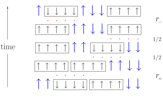
Figure 2: Schematic random walk of irreducible characters for $k=4$ and $L=12$ with PBC’s. The deletion procedure described in the text is here depicted by the boxes around reducible groups of spins. At each step the identification of these latter is made, say, from left to right. Larger spins denote the irreducible characters whose ordering is left invariant by the dynamics. Dots signal the locations of updated spins with rates indicated at the rightmost column (see Eq. (II) and Fig. 1).

Due to the highly convoluted form in which that sequence is obtained, it is clear that $k$ parallel spins well separated from each other may or may not form a reducible $k$-mer depending on the substrings in between. In that sense, the IS conservation is non-local as it involves the whole configuration. More importantly, as mentioned in Ref. Barma2 note that two spin configurations $|S\rangle,\,|S^{\prime}\rangle$ are connected by the dynamics $\Longleftrightarrow I\{S\}=I\{S^{\prime}\}$. As long as all AD rates are held finite, evidently this also applies in the presence of interactions at $T>0$. Thus, the IS uniquely labels all subspaces left invariant by the $k$-mer dynamics, and regardless in which order the reducible groups are removed. In particular, for $k>2$ the AF state is therefore unreachable either from initially empty or closed packed chains as these latter belong to NS sectors, whereas an AF configuration is already irreducible. We will further discuss this issue in Sec. III C when characterizing the actual ground state in NS spaces for $J<0$.

Now it is clear that the number of combinations forming all irreducible sequences for $k>2$ grows exponentially with the number of characters or string length ${\cal L}\leq L$ (with ${\cal L}\propto k$). More specifically, a straightforward analysis of a recursive relation for this $\cal L$- dependent quantity Barma1 ; Barma2 , shows that for large ${\cal L}$ and $k>2$ the number of invariant subspaces or string sectors increases as fast as $x^{\cal L}\!$, with $x$ being the largest root of $x^{k}=2\,x^{k-1}-1$. As for dimers, where this AD process reduces to a spin exchange kinetics note1 , it is worth pointing out that although the IS construction is still well defined, in this case all strings simply consist of AF sequences of lengths ${\cal L}=L,L-2,\cdots,2,0$; each one (except ${\cal L}=0$) having two possible orientations. So, these $L+1$ strings just correspond to each of the $\pm\cal L$ total magnetizations left invariant by the Kawasaki dynamics.

II.2 Kink representation

Turning to the evolution operator, it is convenient at this point to move to the domain wall or kink representation, so as to halve the dimensions of the stochastic matrix in the diagonalizations of Sec. III. In that two-to-one mapping (outlined before in Fig. 1), new Ising variables $\sigma_{i}\equiv-S_{i}\,S_{i+1}$ with energy $E_{\sigma}=J\sum_{i}\sigma_{i}$  stand on dual chain locations where pairing and diffusion of kinks ($\sigma=1$) may take place. Such dual processes can then be schematized as

$$r_{\!{}_{+}}$$

$$1\;\underbracket{\circ\cdots\,}_{k-1}\;1\;\; \underbracket{\rightleftarrows}_{r_{\!{}_{-}}} \;\;\circ\;\,\underbracket{\circ\cdots\,}\;\circ\;\;\;\;\,({\rm pairing}\,,\;\Delta E=\mp 4J)\,,$$ (9a)

$$1\;\underbracket{\circ\cdots\,}_{k-1}\;\circ\;\, \underbracket{\rightleftarrows}_{1/2} \;\;\circ\;\,\underbracket{\circ\cdots\,}\,1\;\;\;\;\;({\rm diffusion}\,,\;\Delta E=0)\,,$$ (9b)

with all brackets involving $k\!-\!1$ vacancies ($\sigma=\!-1$) in the dual chain. Now, thinking of these kink configurations as 1/2- spinors states $|\,\sigma\,\rangle\equiv|\,\sigma_{1},\cdots\sigma_{L}\,\rangle$ (say in the $z$ direction), clearly these processes can be associated with the action of usual raising and lowering operators $\sigma^{+},\sigma^{-}$. More specifically, introducing the projectors

$$\hat{P}_{i}^{(k)}=\frac{1}{2^{k-1}}\;\prod_{j=1}^{k-1}\,(1-\sigma^{z}_{i+j})\,,$$ (10)

[ here playing the role of the Kronecker delta in Eq. (II) ], so as to allow transitions mediated only by empty intervals $[\,i\!+\!1\,,i\!+\!k-1\,]$, then the operational nondiagonal counterparts of Eq. (2a) accounting for both pairing and diffusion events sketched in (9), are respectively given by

$$H_{nd}^{{}^{(pair)}} = -\sum_{i}\,\hat{P}_{i}^{(k)}\left(\,r_{\!{}_{-}}\,\sigma^{+}_{i}\,\sigma^{+}_{i+k}\,+\,r_{\!{}_{+}}\,\sigma^{-}_{i}\,\sigma^{-}_{i+k}\,\right)\,,$$ (11a)

$$H_{nd}^{{}^{(di\!f\!f)}} = -\frac{1}{2}\,\sum_{i}\,\hat{P}_{i}^{(k)}\left(\,\sigma^{+}_{i}\,\sigma^{-}_{i+k}+{\rm H.c.}\,\right)\,.$$ (11b)

Although this would leave us with a nonsymmetric evolution operator, we can now exploit detailed balance to bring Eq. (11a) into a symmetric form. In this context this amounts to considering the nonunitary spin rotation

$$R=\exp\Big{(}-i\frac{\varphi}{2}\sum_{j}\sigma^{z}_{j}\,\Big{)}\,,$$ (12)

with pure imaginary angles $\varphi=iK$. Since $R$ is diagonal and its matrix elements $\langle\,\sigma\,|\,R\,|\,\sigma\rangle=e^{\,\frac{\beta}{2}E_{\sigma}}$ just involve the above kink energies, then all transition rates derived from Eq. (2a) will transform as

$$W(\sigma\to\sigma^{\prime})\to e^{\,{\frac{\beta}{2}}\,\left(E_{\sigma^{\prime}}-E_{\sigma}\right)}\,W(\sigma\to\sigma^{\prime})\,.$$ (13)

Taking into account that $W(\sigma\to\sigma^{\prime})$ also comply with detailed balance [ Eq. (4) ], it is thus clear that in the transformed representation all these nondiagonal elements become symmetrical, i.e. $W(\sigma\to\sigma^{\prime})\to[\,W(\sigma\to\sigma^{\prime})\;W(\sigma^{\prime}\to\sigma)\,]^{1/2}$. In particular, under the spin rotation (12) the pairing terms of Eq. (11a) transform as

$$r_{\!{}_{\mp}}\,\sigma^{\pm}_{i}\,\sigma^{\pm}_{i+k}\,\to\,\frac{1}{2}\;{\rm sech}\,2K\;\sigma^{\pm}_{i}\,\sigma^{\pm}_{i+k}\,,$$ (14)

while leaving projectors (10) and all diffusion terms of Eq. (11b) unchanged. Thus, collecting the contributions of $H_{nd}^{{}^{(pair)}}\!\!+H_{nd}^{{}^{(di\!f\!f)}}\!\!\!$, the symmetrized operational analog of Eq. (2a) is now given by

$$H_{nd}^{(k)}=-\frac{1}{4}\,(1+{\rm sech}\,2K)\,\sum_{i}\,\hat{P}_{i}^{(k)}\left(\,\sigma^{x}_{i}\,\sigma^{x}_{i+k}+\tanh^{2}\!K\;\sigma^{y}_{i}\,\sigma^{y}_{i+k}\,\right)\,.$$ (15)

To complete the construction of the evolution operator, we last turn to the diagonal matrix elements of Eq. (2b) needed for conservation of probability. By definition, these elements count the number of weighted manners in which a given configuration $|\,\sigma\,\rangle$ can evolve to different ones either in one pairing or diffusion step. As before, this can be tracked down in terms of the above $\hat{P}_{i}^{(k)}\!$ projectors, while concurrently probing the appropriate occupancy of kinks and vacancies at sites $i,i+k$. So, in adding those diagonal contributions the counterpart of Eq. (2b) becomes

$$H_{d}^{(k)}=\frac{1}{2}\,\sum_{i}\,\hat{P}_{i}^{(k)}\Big{[}\,1+\,\frac{1}{2}\,\tanh 2K\,\big{(}\sigma^{z}_{i}+\sigma^{z}_{i+k}\big{)}\,\Big{]}\,,$$ (16)

which in turn is left invariant by the spin rotation (12). It is worth noting that for $k=1$ (Glauber dynamics) no projectors are necessary and $H_{nd}+H_{d}$ fully recovers the bilinear form of Ref. Glauber , being ultimately reducible to a free fermion Hamiltonian. By contrast, for $k>1$ projectors (10) introduce correlated pairing and hopping terms as well as many-body interactions, in which case the evolution operator is no longer soluble (cf. however Fig. 4a in Sec. III A).

As for the string sectors obtained from the reduction rules Barma2 summarized in Sec. II A, it can be readily checked that in the dual representation those reductions amount to deleting $k$- contiguous vacancies ( $\circ\cdots^{\!\!\!\!\!{}^{k}}\;\circ\to\emptyset$ ), along with replacing kink pairs with $k\!-\!1$ vacancies in between by just one vacancy ( $1\circ\cdots^{\!\!\!\!\!\!\!\!\!{}^{k-1}}1\to\circ$ ). As a result of the repeated applications of these reductions one is left with string sequences of length ${\cal L}\propto k$ where there can be no more than $k-2$ consecutive vacancies, each sequence being left invariant by the dual dynamics. In practice, to deploy a complete set of NS configurations (where the diagonalizations of Sec. III are carried out), we shall successively apply Eq. (15) to the states stemming from an initial one in that sector until this latter is exhausted.

III Numerical results

Armed with $H^{(k)}\equiv H_{nd}^{(k)}+H_{d}^{(k)}$ acting on generic kink states, we can now implement a Lanczos diagonalization procedure Lanczos without having to store in memory the matrix representation of the evolution operator. As mentioned in Sec. I, we focus on the NS sector ($S_{\emptyset}$) containing the initially empty chain and restrict ourselves to the cases of $k=3$ and 4. Firstly, as a consistency check, we verified that transforming the Boltzmann distribution $R\,|P_{B}\rangle\propto\sum_{\sigma}\exp(-\frac{\beta}{2}E_{\sigma})|\,\sigma\rangle$ with rotation (12) and $|\sigma\rangle\in S_{\emptyset}$, actually produces a ground state of $H^{(k)}$ with eigenvalue $\lambda_{0}\equiv 0$. This also served to start up the Lanczos recursion but with a random initial state chosen orthonormal to that equilibrium direction. In turn, all subsequent states generated by the Lanczos algorithm were also reorthogonalized to $R\,|P_{B}\rangle$. Thereafter, we obtained the first excited eigenmodes of $H^{(k)}$ for lengths of up to $L=30$ for $k=3$ and $L=36$ for $k=4$, the main limitation for this being the exponential growth of the space dimensionality in $S_{\emptyset}$ Barma2 .

III.1 Ferromagnetic case

In this situation, after a quench to low-temperature regimes the large-time dynamics of $S_{\emptyset}$ is essentially mediated by kinks that diffuse at no energy cost (rate 1/2). Owing to the projectors of Eqs. (11a) and (11b) however note that kinks can not cross each other, neither annihilate in the presence of other kinks in between, nor if they diffuse through different sublattices. But taking into account the reduction rules referred to in Sec. II B for the dual representation, there must be at least one interval with two kinks separated by $nk-1$ vacancies ($1\leq n\leq\frac{L}{k}-1$); otherwise the explored configurations would not be fully reducible to $S_{\emptyset}$. Hence, there are regions where kinks can always meet at a distance of $k$ lattice spacings and annihilate in pairs ($\Delta E=-4J$) with rate $r_{\!{}_{+}}\lesssim 1$, which in the limit of $T\to 0$ gives rise to a monotonic coarsening of F domains. Therefore, close to the equilibrium regime of $S_{\emptyset}$ the characteristic time involved between pair annihilations is that for kinks to diffuse across a correlation length $\xi\propto L$, so a relaxation time $\tau$ growing as $L^{2}$ might be expected.

In fact, this is evidenced in Figs. 3(a) and 3(b) where scaling plots of the spectral gaps ($\lambda_{1}=1/\tau$) of $H^{(k)}$ are shown for $k=3$ and 4 respectively. As temperature is lowered the data collapse towards larger sizes is attained on choosing a diffusive dynamic exponent ($z=2$). This is also in close agreement with the slopes read off from the insets, in turn estimating these finite-size gaps in their low temperature limit [ $\lambda_{1}^{\!{}^{*}}(L):=\lim_{\,T\to 0}\,\lambda_{1}(L)$ ].

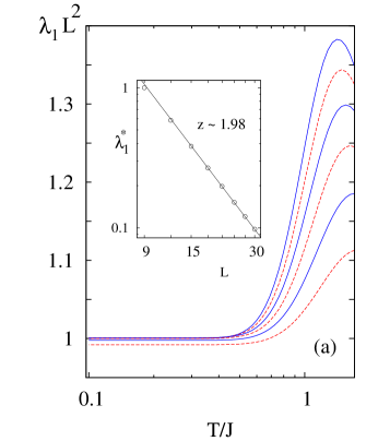
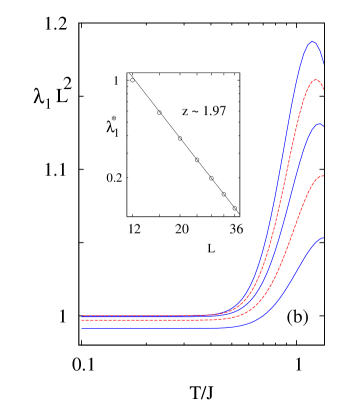
Figure 3: Finite-size scaling of spectral gaps of the evolution operator ($J>0$) on approaching low-temperature regimes in NS sectors for (a) $k=3$, and (b) $k=4$. From top to bottom solid and dashed lines stand in turn for sizes $L\propto k$ with (a) $L=30,\cdots,15$, and (b) $L=36,\cdots,20$. The slopes of the insets estimate the typical finite-size decay of these gaps in the limit of $T\to 0$, thus suggesting a common dynamic diffusive exponent. For displaying convenience, in (a) and (b) the vertical scales of main panels were normalized by factors $30^{2}\,\lambda_{1}^{\!{}^{*}}(30)$ and $36^{2}\,\lambda_{1}^{\!{}^{*}}(36)$ respectively.

Moreover, let us now consider Fig. 4(a) and compare the spectral gaps of the Glauber dynamics Glauber , i.e. $\lambda_{1}(L)=2\,\big{(}1-\tanh 2K\,\cos\frac{\pi}{L}\big{)}$, with those resulting from our finite-size diagonalizations for $k=2,3$, and 4. Interestingly, it turns out that in lowering the temperature $\lambda_{1}(L,k)$ converges towards the exact solution of $k=1$ so long as the length of this latter case is rescaled as $L/k$, i.e. $\lambda_{1}^{\!{}^{*}}(L,k)=2\,\big{(}1-\cos\frac{\pi k}{L}\big{)}$. In particular, for $T/J\lesssim 0.25$ we checked out that for all sizes in reach these gaps become numerically indistinguishable, at least within quadruple precision. Therefore, as far as the critical dynamics is concerned, when $L\gg k$ these comparisons strongly suggest that in the NS sector the fundamental scaling relation between $\tau$ and $L$ is just a diffusive one; more specifically

$$\tau=\Big{(}\frac{L}{\pi k}\Big{)}^{2}+{\cal O}(1)\,.$$ (17)

In passing note that for $k=2$ where, as mentioned before, the problem reduces to a Kawasaki dynamics with $J<0$ (no metastability), this diffusive picture is consistent with the results encountered in previous studies Lage .

Now we check whether this length resizing is of any consequence on a more microscopic level of description, such as the equal-time two-point correlators $C_{k}(r,t)=\frac{1}{L}\sum_{j}\langle S_{j}\,S_{j+r}\rangle(t)$ in the original spin representation. In Fig. 4 (b) we display these functions in the NS sectors of several $k$-mers by simulating quenches down to $T=0$ from initially disordered states.

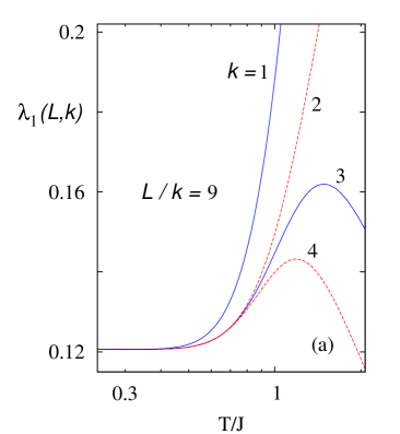
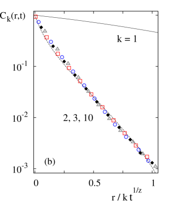
Figure 4: (a) Low-temperature scaling of spectral gaps ($J>0$) for several $k$-mer sizes. As $T\to 0$, all gaps collapse onto the exact solution of the monomer case (Glauber dynamics), provided the chain length of this latter is rescaled by a factor $1/k$. Other reachable values of $L/k$ (not shown) also follow the Glauber solution in that limit. (b) Scaling plot of spin-spin correlation functions ($J>0$) for $L=1.2\times 10^{5}$ after a quench down to $T=0$. The data collapse was attained upon renormalizing $r$- distances as $r/k$ while choosing dynamic exponents $z\in(1.96\,,\,2.07)$. Squares ($t=5\times 10^{3}$ steps) and circles ($t=5\times\!10^{4}$) depict the case $k=3$, whereas rhomboids ($t=10^{3}$) and triangles ($t=10^{4}$) stand for $k=10$. Error bars are smaller than twice the symbol sizes. The dashed line represents the case $k=2$ after $10^{4}$ steps, while the solid one denotes the exact scaling function of Ref. Bray .

For $k>2$ the sampling of these latter poses the nontrivial problem of generating an equally weighted distribution of NS configurations. As an approximation though, here each disordered sample was obtained by evolving the AD process through $10^{6}$ steps in the high temperature limit ($J=0$), starting from $L/k$ consecutive $k$-mers randomly oriented (particle or vacancy). On par with Fig. 4(a), it turns out that after averaging over $\sim 3\times 10^{3}$ independent samples in chains with $1.2\times 10^{5}$ sites, there is a common scaling form into which these correlators can be made to collapse provided all spin separations are rescaled as $r/k$,  i.e. $C_{k}(r,t)\simeq F\big{(}r/\;k\,t^{1/2}\big{)}$. For monomers, where there is no equivalent to the IS construction neither conserved quantities, an exact scaling form for these correlators can be cast in terms of the complementary error function, namely Bray

$$C_{1}(r,t)={\rm erfc}\big{(}\,r/\;2\,t^{1/2}\big{)}\,,$$ (18)

although as is shown in Fig. 4(b), it is rather apart from the other $k$-mer cases. Nonetheless, and in line with Eq. (17), clearly all these AD situations are characterized by ferromagnetic length scales coarsening as $k\,t^{1/2}$.

III.2 Antiferromagnetic case

By contrast to the F dynamics, under AF interactions often this system can reach states in which further energy-lowering processes are unlikely at low temperature regimes. These configurations are such that there can be no more than $k$- consecutive parallel spins, and proliferate exponentially with $L$. Although the AF dynamics attempts to maximize the number of kinks, note that once one of these states is reached there is no way to escape from it without first annihilating a kink pair ($\Delta E=-4J$). If that annihilation in turn produces at least $2k+1$ parallel spins, then by subsequent diffusion of kinks eventually a domain of $2k+3$ spins can be accommodated at no further energy cost. A scheme of this decay process, say for $k=3$, is depicted in Fig. 5.

Figure 5: Schematic decay from a trimer metastable state (top) under $J<0$. After surmounting the initial energy barrier, kinks separating opposite spin orientations can diffuse freely until an interval of nine parallel spins shows up. This allows to decrease the initial energy by creating two kink pairs (bottom). Brackets show updated locations, whereas numbers in diffusion events indicate the ordering of those updates.

This prepares the conditions to create two kink pairs with which the original metastable energy is finally lowered in $\Delta E=4J$. As indicated in Fig. 5 note that this also requires the initial presence of at least two $k$-mer locations, no matter how distant they might be note3 . Later on we will make use of this decay pattern when sampling ground states of larger chains (Sec. III C).

At infinitesimal temperatures note2 and independently of the system size, the activation energies needed for these pair annihilations introduce divergences in the actual relaxation times via the Arrhenius factors $\propto e^{-4J/T}$ mentioned in Sec. I. In estimating dynamic exponents from exact diagonalizations it is then natural to use the finite-size scaling hypothesis referred to in Eq. (1), which in terms of ’normalized’ spectral gaps reads

$$\Lambda_{1}^{\!{}^{*}}(L)\equiv\lim_{T\to 0^{+}}e^{\,-4J/T}\,\lambda_{1}(L)\,\propto L^{-z}.$$ (19)

However, as temperature is lowered the spacing of the low-lying levels of the evolution operator gets arbitrarily small, so in practice it turns out that the pace of the Lanczos convergence becomes prohibitively slow for $T/|J|\lesssim 0.15$. Nevertheless, a clear saturation trend already shows up for our lowest accessible $T$’s, thus signaling the entrance to the Arrhenius regime, and within which the normalized gaps are then scaled with the system size. This is exhibited in Figs. 6(a) and 6(b)

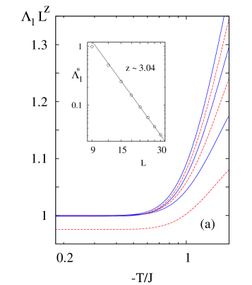
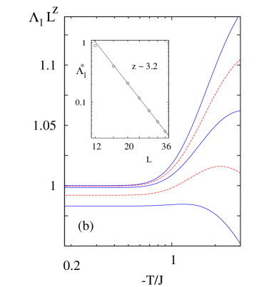
Figure 6: Scaling of normalized gaps [ Eq. (19), $L\propto k$ ] for NS spaces and $J<0$. Solid and dashed lines in upward order show alternately the cases of (a) $L=15,\cdots,30$ for $k=3$, and (b) $L=20,\cdots,36$ for $k=4$. The data collapse in the low-temperature regime was obtained using dynamic exponents read off from the slope of the insets (also see Table 1). Just as in Fig. 3, for displaying convenience the vertical scales of main panels were respectively normalized by factors $30^{z}\,\Lambda_{1}^{\!{}^{*}}(30)$ and $36^{z}\,\Lambda_{1}^{\!{}^{*}}(36)$. The $\Lambda_{1}\!$ plateaus are consistent with the Arrhenius regimes referred to in the text.

for the NS sectors of $k=3$ and 4 respectively. Note that even a slight deviation from the conjectured energy barriers would result in strong departures from those $\Lambda_{1}\!$ plateaus. More importantly, the finite-size decay of these quantities within that region is indicative of dynamic exponents rather different from the diffusive ones obtained under F couplings. Their values are estimated by the slopes shown in the insets, and produce the collapse of larger size data in nearing the Arrhenius regime. A more detailed trend of size effects on these subdiffusive exponents is provided by the sequence of effective approximants

$$Z_{L}(k)=\frac{\ln\big{[}\,\Lambda_{1}^{\!{}^{*}}(L)/\Lambda_{1}^{\!{}^{*}}(L-k)\,\big{]}}{\ln\big{[}\,(L-k)/L\,\big{]}}\,,$$ (20)

which simply derives a measure of $z(k)$ from the gaps of successive chain lengths $\propto k$. In Table 1 we list our higher approximants which happen to come out as forming sequences of upper and lower bounds for $z(3)$ and $z(4)$ respectively.

$L/k$	$Z_{L}\,(k=3)$	$Z_{L}\,(k=4)$
7	3.0713	3.1558
8	3.0662	3.1887
9	3.0577	3.2117
10	3.0431

Table 1: Convergence of dynamic exponents as resulting from the slopes between larger available sizes in the insets of Fig. 6.

The case of trimers seems to converge towards a Lifschitz-Slyozov behavior [ $\xi(t)\propto t^{1/3}$ ], similar to that encountered in the ferromagnetic 1D Kawasaki dynamics Cornell as well as in $d\geq 2$ by surface dynamical arguments Huse . As already pointed out, the connection to the Kawasaki dynamics stems from its mapping to the dimer case, though with opposite coupling signs note1 . It is then interesting to check that either under AF or F couplings the dynamic exponents of the trimer case ($z\simeq 3$ and 2 respectively), also follow those of the corresponding dimer (Kawasaki) kinetics. This common behavior of dimers and trimers contrasts with that of the case of $J=0$ where it was found that their autocorrelation functions in NS sectors decay in time with different power laws Barma1 ; Barma2 . On the other hand, for $k=4$ the approximants of Table 1 suggest a slightly slower kinetics, possibly also implying non-universality on $k$ (contrariwise to the case $J>0$ discussed in Sec. III A).

III.3 Ground state characterization ($J<0$)

Turning to equilibrium at $T=0^{+}$, as stressed by the end of Sec. II A the NS constraint impedes the ordering of AF configurations for $k\geq 3$ when $J<0$. Instead, a highly degenerate structure emerges. It is similar to that of the metastable states described in Sec. III B except in that neither eventual adsorptions nor desorptions of $k$-mers would give rise to more than $2k$ parallel spins. Hence, subsequent diffusion of kinks like those schematized in Fig. 5 could not meet the conditions to reduce the energy further (see discussion below).

When it comes to jamming scales, i.e. distances between flippable $k$-mers or lengths $\xi_{{}_{J}}$ through which there can be at most $k-1$ consecutive parallel spins, we have estimated their growth with $L$ by exact enumerations of ground states in the lattice sizes at reach. Since at finite temperatures the dynamics is ergodic on each subspace, those regions can not remain jammed at all times. However, in the limit of $T\to 0^{+}$ note that the activation barriers referred to in Sec. III B allow those jammed regions to persist for arbitrarily large times in turn $\propto e^{4|J|/T}$. The data exhibited in Fig.  7 are consistent with an average jamming length growing as $\langle\xi_{{}_{J}}\rangle\propto(\ln L)^{1/\alpha}$ with $\alpha\sim 1.6$ for $k=3$, and $\alpha\sim 1.7$ for $k=4$, thus suggesting a small $k$-mer density (active regions). Moreover, the wide-tailed distributions of these lengths (upper insets), indicate the abundance of much broader jamming scales, a situation which is in part reminiscent of that found in RSA processes (cf. Sec. I).

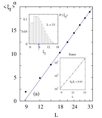
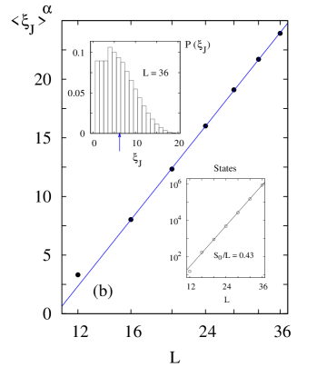
Figure 7: Main panels: logarithmic growth of average jamming lengths $\xi_{{}_{J}}$ with the system size ($L\propto k$) in the ground states of NS sectors with $J<0$ for (a) $k=3$ ($\alpha\simeq 1.6$), and (b) $k=4$ ($\alpha\simeq 1.7$). The distribution of these length scales in our largest accessible chains are shown in the upper histograms. Vertical arrows signal the mean values of $\xi_{{}_{J}}$. Lower insets illustrate the exponential degeneracy of the corresponding ground states. In turn, the slopes indicate a residual entropy per site $S_{0}/L\sim 0.41$ for $k=3$, and $\sim 0.43$ for $k=4$.

As for the high degeneracy of these states, the lower insets of Fig. 7 clearly evidence an exponential growth of their number with the system size, which implies a non-vanishing entropy in the low-temperature limit. In all examined cases the minimum energy is realized by configurations containing $2\left(\frac{L}{k}-1\right)$ kinks subject to the NS constraint.

Owing to the Arrhenius barriers the sampling of ground states in larger chains would be hardly accessible to standard simulations. To bypass this problem, we just implement the decay pattern of the typical metastable configurations considered in Sec. III B, and in particular schematized for the case of trimers in Fig. 5. Firstly, we flip a $k$-mer location regardless of its energy cost while checking that, as a result, at least $2k+1$ parallel spins are left (cf. Fig. 5). Secondly, we allow the dynamics to proceed, but only through kink diffusion ($\Delta E=0$), i.e. avoiding pair creation-annihilation events, until a group of $2k+3$ contiguous parallel spins shows up. As schematized in Fig. 5 this finally permits to reduce the original metastable energy by creating two kink pairs. This rearrangement process is then repeated until there is no longer any $k$-mer whose flip brings about at least $2k+1$ parallel spins. It is this latter feature what actually distinguishes a ground state configuration from a metastable one. Note that if the process were to continue, then subsequent kink diffusion would arrange intervals of at most $2k+2$ parallel spins, and so only one kink pair could be accommodated to compensate the energy excess $(-4J)$ caused by the initial $k$-mer flip. As a result, the system would just be left in another ground state configuration. Thereafter the sampling continues but starting from other independent metastable state, in turn rapidly obtainable from a quench down to $T=0$. As a consistency check, it is worth mentioning that all ground state samples in the NS sector reached a maximum of $2\left(\frac{L}{k}-1\right)$ kinks, which is also in line with that obtained by exact enumeration in much smaller sizes.

The spin correlations $C(r)=\frac{1}{L}\sum_{j}\langle S_{j}\,S_{j+r}\rangle$ for $k=3$ and 4 resulting from this sampling scheme are shown respectively in Figs. 8(a) and 8(b) after decaying from the metastable states generated by $\sim 10^{4}$ independent quenches. The rather large correlation lengths, in turn growing in proportion to the increase of the system size ($\Delta\xi\;\tilde{\propto}\;\Delta L$), presumably indicates long range order in the thermodynamic limit.

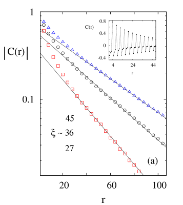
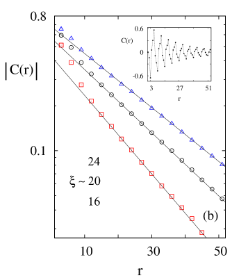
Figure 8: Spin-pair correlations in the ground states of NS sectors $(J<0)$ obtained by the sampling procedure described in the text for (a) $k=3$, and (b) $k=4$. Squares, circles, and triangles stand respectively for $L=600,900,1200$ in (a), and $L=1800,2400,3000$ in (b). Error bars are smaller than twice the symbol sizes. The insets illustrate the cases of largest $L$’s, whereas for displaying clarity only local extrema are shown in main panels. The inverse slopes of solid lines are fitted with correlation lengths $\xi$ which grow with the chain size.

In that sense, it would be desirable to extend this picture to much larger chains, but there our sampling approach becomes progressively impractical. Finally, the insets exhibit the nontrivial forms which the NS constraint ends up imposing on these correlations, their oscillations for $k=3$ and 4 having respectively periods of four and six lattice units.

IV Concluding discussion

To summarize, we have studied the low-temperature and large-time dynamics of extended objects ($k$-mers) which reconstruct and interact while adsorbing/ desorbing in one-dimension. For $k\geq 3$ the notion of irreducible string Barma2 provided an exhaustive description of the unusual manner in which the phase space is divided in sectors left invariant by the dynamics (Sec. II A). Although the number of such subspaces grows exponentially with the substrate size Barma1 ; Barma2 , we restricted the scope of this study to the so called null-string sector (containing the empty lattice configuration), both for computational ease and for being a common starting point in the context of cooperative AD processes Evans .

Thinking of these latter as multi-spin flip dynamics in Ising chains, we have constructed their evolution operators in the dual or kink representation of Sec. II B, by which we analyzed the scaling behavior of relaxation times in finite substrates. The resulting time scales were then read off from the spectral gaps obtained using standard recursive methods Lanczos , ultimately enabling us to estimate dynamic exponents via the finite-size scaling hypothesis (1). In the case of F interactions (Sec. III A), the numerical matching of these gaps in the low-temperature limit with those of the rescaled Glauber operator ($L\to L/k$, Fig. 4a), might come as a bit of a surprise given the many-body correlations introduced by projectors (10) both in paring and hopping terms of Eqs. (11a) and (11b). (Although in the limit of $T\to 0$ the creation of kink pairs is unlikely, the caging effect of those projectors on the remaining kinks is still important as not all of them necessarily move in the same sublattice. Hence, in the null sector, a strict analogy with the rescaled Glauber dynamics is not evident beyond two-kink excitations). The close overlap of those gaps near the critical regime thus strongly suggests a diffusive growth of relaxation times $\forall\,k\geq 1$ [ Eq. (17), and data collapse of Fig. 3 ]. This was also corroborated by simulated quenches of spin-pair correlations (Fig. 4b), in all cases exhibiting ferromagnetic lengths which spread as $\sim k\,t^{1/2}$. Also upon normalizing all pair distances as in Fig. 4a ($r\to r/k$), these correlations were made to collapse into a single scaling function but different from that of the Glauber or monomer case Bray . Whether this is due to the absence of conserved quantities, such as the irreducible strings or the sublattice magnetization differences of Eq. (7), remains an open issue. Let us add that this also might be an outcome of matrix elements of pair correlators being very different for $k>1$ in the eigenstate basis of the evolution operator.

Owing to the metastable states appearing in the AF situation (Sec. III B), simulated quenches become impractical near the Arrhenius regime, so we contented ourselves with the above finite-size scaling methods, this time applied to the normalized gaps of Eq. (19). The scaling plots of these latter (Fig. 6), as well as the sequence of our higher approximants [ Eq. (20) and Table 1 ], are indicative of subdiffusive dynamic exponents well apart from $z=2$. For $k=3$ these seem to belong to the Lifschitz-Slyozov universality class Huse characteristic of the ferromagnetic Kawasaki dynamics Cornell (in this context, formally analogous to that of $k=2$ under $J<0$), although for $k=4$ the approximants of Table 1 suggest a convergence towards a slightly slower dynamics. This nonuniversal aspect clearly deserves further verifications in larger sizes, but already the next effective exponent ($Z_{40}$) would involve diagonalizations in spaces of $\sim 5.02\times 10^{7}$ dimensions.

With further regard to nonuniversality issues, it would be relevant to extend this study to the dynamics of string sectors with finite density of irreducible characters, such as those considered in the noninteracting case of Ref. Barma2 . There it was found that autocorrelation functions exhibit a wide diversity in the manner in which these decay in time, depending on the studied sector. In our case, preliminary diagonalizations for $J>0$ in similar sectors however suggest that the diffusive picture found in Sec. III A still holds, though an understanding of the emergent low-temperature phases (also highly degenerate) would require further investigations.

In the null string subspace with $J<0$ (where AF ordering is unattainable for $k>2$), that latter aspect was addressed in Sec. III C by exact enumerations in small chains alongside with the sampling of ground states in larger substrates. The former approach revealed both the appearance of growing jammed scales and finite residual entropies (Fig. 7), whereas the latter one  -implemented by exploiting the decay pattern of Fig. 5-  disclosed nontrivial spin-pair correlations presumably long ranged in the thermodynamic limit (Fig. 8). As an open problem also remains to elucidate to what extent these features, as well as the dynamic ones of Sec. III B, might be affected by the inclusion of a small magnetic field, i.e. a monomer chemical potential slightly apart from that set by their couplings.

References

- (1) P. J. Flory, J. Am. Chem. Soc. 61, 1518 (1939).
- (2) For reviews, consult J. W. Evans, Rev. Mod. Phys. 65, 128 (1993); V. Privman, Colloids and Surfaces A: Physicochem. Eng. Aspects 165, 231 (2000); V. Privman, Trends Stat. Phys. 1, 89 (1994).
- (3) C. Shen, L.-P. Wang, B. Li, Y. Huang, and Y. Jin, Vadose Zone J. 11(1), (2012). doi:10.2136/vzj2011.0057
- (4) P. Frantz and S. Granick, Phys. Rev. Lett. 66, 899 (1991).
- (5) C.J. Murphy, M.R. Arkin, Y. Jenkins, N.D. Ghatlia, S.H. Bossmann, N.J. Turro, and J.K. Barton, Science 262, 1025 (1993).
- (6) Nonequilibrium Statistical Mechanics in One Dimension, edited by V. Privman (Cambridge University Press, UK, 1997).
- (7) M. Barma, M. D. Grynberg, and R. B. Stinchcombe, Phys. Rev. Lett. 70, 1033 (1993); R. B Stinchcombe , M. D. Grynberg, and M. Barma, Phys. Rev. E 47, 4018 (1993).
- (8) M. Barma and D. Dhar, Phys. Rev. Lett. 73, 2135 (1994); D. Dhar and M. Barma, Pramana–J. Phys. 41, L193 (1993); M. Barma, ibid. 49, 155 (1997); see also M. Barma in Ref. Privman .
- (9) I. Mazilu, D. A. Mazilu, R. E. Melkerson, E. Hall-Mejia, G. J. Beck, S. Nshimyumukiza, and C. M. da Fonseca, Phys. Rev. E 93, 032803 (2016); L. J. Cook, D. A. Mazilu, I. Mazilu, B. M. Simpson, E. M. Schwen, V. O. Kim, and A. M. Seredinski, Phys. Rev. E 89, 062411 (2014).
- (10) N. G. van Kampen, Stochastic Processes in Physics and Chemistry, 3rd ed. (North-Holland, Amsterdam, 2007), Chap. 5.
- (11) R. J. Glauber, J. Math. Phys. 4, 294 (1963); B. U. Felderhof, Rep. Math. Phys. 1, 215 (1971).
- (12) K. Kawasaki, in Phase Transitions and Critical Phenomena, edited by C. Domb and M. S. Green (Academic Press, London,1972), Vol. 2; K. Kawasaki, Phys. Rev. 145, 224 (1966).
- (13) This just follows from the spin mapping , say at even locations, while leaving the odd spins unchanged. Then whereas dimer deposition-evaporation is represented as a spin exchange between neighboring sites.
- (14) P. C. Hohenberg and B. Halperin, Rev. Mod. Phys. 49, 435 (1977).
- (15) For further reviews, see Kinetics of Phase Transitions, edited by S. Puri and V. Wadhawan (CRC Press, Boca Raton, FL, 2009); A. J. Bray, Adv. Phys. 43, 357 (1994).
- (16) Consult for instance, M. Henkel, H. Hinrichsen, and S. Lübeck, Non-Equilibrium Phase Transitions (Springer, Dordrecht, 2008), Vol. 1, Appendix F.
- (17) C. Monthus and T. Garel, J. Stat. Mech. (2013) P02037; R. B. Stinchcombe, Adv. Phys. 50, 431 (2001); M. D. Grynberg, in Annual Reviews of Computational Physics, edited by D. Stauffer (World Scientific, Singapore, 1996), Vol. 4.
- (18) See for example, G. H. Golub and C. F. van Loan, Matrix Computations, 3rd ed. (Johns Hopkins University Press, Baltimore, 1996), Chap. 9; Y. Saad, Numerical Methods for Large Eigenvalue Problems, 2nd ed. (SIAM, Philadelphia, 2011), Chap. 6.
- (19) For finite-size diagonalizations in this context of invariant string sectors see also P. B. Thomas, M. K. Hari Menon, and D. Dhar, J. Phys. A 27, L831 (1994); M. K. Hari Menon and D. Dhar, J. Phys. A 28, 6517 (1995); M. D. Grynberg, Phys. Rev. E 76, 031605 (2007).
- (20) At the dynamics rapidly gets stuck in metastable states, thus preventing the system to reach equilibrium.
- (21) However, if the targeted -mer happens to be contiguous to another one, then at least a third -mer location is needed.
- (22) M. Suzuki and R. Kubo, J. Phys. Soc. Jpn. 24, 51 (1968).
- (23) J. M. Nunes da Silva and E. J. S. Lage, Phys. Rev. A 40, 4682 (1989); J. H. Luscombe, Phys. Rev. B 36, 501 (1987); M. K. Phani, J. L. Lebowitz, M. H. Kalos, and O. Penrose, Phys. Rev. Lett. 45, 366 (1980).
- (24) A. J. Bray, J. Phys. A 22, L67 (1990); see also A. J. Bray in Ref. Privman .
- (25) S. J. Cornell, K. Kaski, and R. B. Stinchcombe, Phys. Rev. B 44, 12263 (1991).
- (26) D. A. Huse, Phys. Rev. B 34, 7845 (1986) ; I. M. Lifshitz and V. V. Slyozov, J. Chem. Solids 19, 35 (1961).