Action Growth in $f\left(R\right)$ Gravity

Abstract

Inspired by the recent “Complexity = Action” conjecture, we use the approach proposed by Lehner et al. to calculate the rate of the action of the WheelerDeWitt patch at late times for static uncharged and charged black holes in $f\left(R\right)$ gravity. Our results have the same expressions in terms of the mass, charge, and electrical potentials at the horizons of black holes as in Einstein’s gravity. In the context of $f\left(R\right)$ gravity, the Lloyd bound is saturated for uncharged black holes but violated for charged black holes near extremality. For charged black holes far away from the ground states, the Lloyd bound is violated in four dimensions but satisfied in higher dimensions.

I Introduction

Recently, Brown et al. IN-Brown:2015bva ; IN-Brown:2015lvg proposed the “Complexity = Action” (CA) duality, which conjectures that the computational complexity $\mathcal{C}$ of a holographic boundary state could be identified with the classical gravitational action $S_{\text{WdW}}$ of the WheelerDeWitt patch:

$$\mathcal{C=}\frac{S_{\text{WdW}}}{\pi\hbar}.$$ (1)

The WheelerDeWitt patch is defined as the domain of dependence of any Cauchy surface anchored at the boundary state. Loosely speaking, the complexity $\mathcal{C}$ of a state is the minimum number of quantum gates to prepare this state from a reference state IN-Wat:2009 ; IN-Huang:2015 ; IN-Osb:2011 . The CA duality is the refined version of the “Complexity = Volume” duality IN-Susskind:2014rva ; IN-Stanford:2014jda ; IN-Susskind:2014jwa ; IN-Susskind:2014moa , which states that the complexity of a boundary state is dual to the volume of the maximal spatial slice crossing the Einstein-Rosen bridge anchored at the boundary state. Later, the “Complexity = Volume 2.0” duality was proposed in IN-Couch:2016exn , in which the complexity was identified with the spacetime volume of the WheelerDeWitt patch.

After calculating the action growth $dS_{\text{WdW}}/dt$ for various stationary AdS black holes in IN-Brown:2015lvg , Lehner et al. IN-Lehner:2016vdi carefully analyzed the action of some subregion with null segments and joints at which a null segment was joined to another segment. A set of rules for calculating the contributions from these joints were also given in IN-Lehner:2016vdi . Although the two approaches in IN-Brown:2015lvg and IN-Lehner:2016vdi look quite different, they gave the same results for various black holes within Einstein’s gravity IN-Lehner:2016vdi . Beyond Einstein’s gravity, the action growth was calculated by the method of IN-Brown:2015lvg in cases of Gauss-Bonnet gravity IN-Cai:2016xho , massive gravities IN-Pan:2016ecg , $f\left(R\right)$ gravity IN-Alishahiha:2017hwg , and critical gravities IN-Alishahiha:2017hwg . On the other hand, following the method of IN-Lehner:2016vdi , the action growth was calculated for Born-Infeld black holes IN-Cai:2017sjv ; IN-Tao:2017fsy , charged dilaton black holes IN-Cai:2017sjv , and charged black holes with phantom Maxwell field IN-Cai:2017sjv in AdS space. Moreover, the divergent terms of $S_{\text{WdW}}$ due to the infinite volume near the boundary of AdS space were considered in IN-Carmi:2016wjl ; IN-Reynolds:2016rvl ; IN-Kim:2017lrw , where it showed that these terms could be written as local integrals of boundary geometry.

One of the simplest modifications to Einstein’s gravity is the $f\left(R\right)$ gravity IN-Bergmann:1968ve ; IN-Capozziello:2009nq ; IN-Capozziello:2011et ; IN-Nojiri:2010wj in which the Lagrangian density $f$ is an arbitrary function of $R$, where $R$ is the Ricci scalar. It can be shown that the metric-$f\left(R\right)$ gravity is equivalent to the $\omega_{\text{BD}}$ $=0$ Brans-Dicke theory with the potential IN-DeFelice:2010aj . In IN-Alishahiha:2017hwg , the action growth for static uncharged black holes in $f\left(R\right)$ gravity was calculated using the method of IN-Brown:2015lvg . It is interesting to calculate the action growth in $f\left(R\right)$ gravity using the method of IN-Lehner:2016vdi and then check whether these two results are same. In this paper, we will employ the approach proposed in IN-Lehner:2016vdi to compute $dS_{\text{WdW}}/dt$ at late times for static uncharged and charged black holes in $f\left(R\right)$ gravity.

The remainder of our paper is organized as follows: In section II, we discuss the boundary terms in the action functional of $f\left(R\right)$ gravity when the boundary includes null segments. In order to employ the method of IN-Lehner:2016vdi , we consider the Einstein frame representation of the action of a Brans-Dicke theory with Brans-Dicke parameter $\omega_{\text{BD}}=0$, which is dynamically equivalent to the metric-$f\left(R\right)$ gravity. In section III, the action growth of the WheelerDeWitt patch is calculated in the cases of static uncharged and charged black holes in $f\left(R\right)$ gravity. In section IV, we conclude with a brief discussion of our results.

II Action in $f\left(R\right)$ Gravity

The action that defines $f\left(R\right)$ gravity has the generic form

$$S=\int d^{d+1}x\sqrt{-g}f\left(R\right)+S^{m}\left(g_{\mu\nu},\psi\right)\text{,}$$ (2)

where $S^{m}$ is the matter action, $\psi$ is the matter field, and we take $16\pi G=1$. The gravitational equation can be derived by varying the action $\left(\ref{eq:action}\right)$ with respect to $g_{\mu\nu}$:

$$f^{\prime}\left(R\right)R_{\mu\nu}-\frac{1}{2}f\left(R\right)g_{\mu\nu}+\left(g_{\mu\nu}\nabla^{2}-\nabla_{\mu}\nabla_{\nu}\right)f^{\prime}\left(R\right)=\frac{1}{2}T_{\mu\nu}^{m},$$ (3)

where $T_{\mu\nu}^{m}$ is the energy-momentum tensor of the matter field defined by

$$T_{\mu\nu}^{m}=-\frac{2}{\sqrt{-g}}\frac{\delta S^{m}}{\delta g^{\mu\nu}}.$$ (4)

Introducing a new field $\chi$, we could rewrite the action $\left(\ref{eq:action}\right)$ as a dynamically equivalent action:

$$S=\int d^{d+1}x\sqrt{-g}\left[f^{\prime}\left(\chi\right)\left(R-\chi\right)+f\left(\chi\right)\right]+S^{m}\left(g_{\mu\nu},\psi\right).$$ (5)

Varying the action $\left(\ref{eq:actionx}\right)$ with respect to $\chi$ gives

$$f^{\prime\prime}\left(\chi\right)\left(R-\chi\right)=0.$$ (6)

Therefore, $\chi=R$ if $f^{\prime\prime}\left(\chi\right)\neq 0$, which reproduces the action $\left(\ref{eq:action}\right)$. With $\chi=R$, the equation of motion (EOM) obtained by vary the action $\left(\ref{eq:actionx}\right)$ with respect to $g_{\mu\nu}$ recovers eqn. $\left(\ref{eq;EOM}\right)$. Redefining $f^{\prime}\left(\chi\right)$ as a field, it shows that the action $\left(\ref{eq:actionx}\right)$ is the Jordan frame representation of the action of a Brans-Dicke theory with Brans-Dicke parameter $\omega_{\text{BD}}=0$. To diagonalizes the gravi-$\chi$ kinetic term, we introduce the rescaled metric $\tilde{g}$ in the $\tilde{x}$ coordinate:

$$\tilde{g}_{\tilde{\mu}\tilde{\nu}}d\tilde{x}^{\tilde{\mu}}d\tilde{x}^{\tilde{\nu}}=f^{\prime}\left(\chi\right)^{\frac{2}{d-1}}g_{\mu\nu}dx^{\mu}dx^{\nu}.$$ (7)

The action $\left(\ref{eq:actionx}\right)$ then becomes

$$S =\int d^{d+1}\tilde{x}\sqrt{-\tilde{g}}\tilde{R}+\frac{\sqrt{2d}}{\sqrt{d-1}}\int d^{d+1}\tilde{x}\sqrt{-\tilde{g}}\tilde{\nabla}^{2}\phi$$

$$-\frac{1}{2}\int d^{d+1}\tilde{x}\sqrt{-\tilde{g}}\left\{\left(\tilde{\nabla}\phi\right)^{2}+2f^{\prime}\left(\chi\right)^{-\frac{d+1}{d-1}}\left[f^{\prime}\left(\chi\right)\chi-f\left(\chi\right)\right]\right\}+S^{m}\left[f^{\prime}\left(\chi\right)^{-\frac{2}{d-1}}\tilde{g}_{\tilde{\mu}\tilde{\nu}},\psi\right],$$ (8)

where

$$\phi=\sqrt{\frac{2d}{d-1}}\ln f^{\prime}\left(\chi\right).$$

Now consider the action $\left(\ref{eq:actionE}\right)$ over a region $\mathcal{V}$ of spacetime with the boundary $\partial\mathcal{V}$. Since there are second derivatives of the metric tensor and the field $\phi$ in the first line of eqn. $\left(\ref{eq:actionE}\right)$, extra boundary terms need to be added to derive the EOMs from the action. The $\tilde{\nabla}^{2}\phi$ term in eqn. $\left(\ref{eq:actionE}\right)$ can be expressed as a boundary term via Stokes’s theorem:

$$\int_{\mathcal{V}}d^{d+1}\tilde{x}\sqrt{-\tilde{g}}\tilde{\nabla}^{2}\phi=\int_{\partial\mathcal{V}}d^{d}\tilde{x}\sqrt{\left|\tilde{h}\right|}n^{\tilde{\mu}}\tilde{\nabla}_{\tilde{\mu}}\phi,$$ (9)

where $\tilde{h}_{\tilde{\mu}\tilde{\nu}}$ is the induced metric on $\partial\mathcal{V}$, and $n^{\tilde{\mu}}$ is the unit vector normal to $\partial\mathcal{V}$. To have the EOMs by variation of action, this boundary term should be canceled against by another one

$$S_{\partial\mathcal{V}}^{\phi}=-\frac{\sqrt{2d}}{\sqrt{d-1}}\int_{\partial\mathcal{V}}d^{d}\tilde{x}\sqrt{\left|\tilde{h}\right|}n^{\tilde{\mu}}\tilde{\nabla}_{\tilde{\mu}}\phi.$$ (10)

The first term in eqn. $\left(\ref{eq:actionE}\right)$ is just the standard Hilbert action in terms of $\tilde{g}_{\tilde{\mu}\tilde{\nu}}$, which contains second derivatives of $\tilde{g}_{\tilde{\mu}\tilde{\nu}}$ and hence requires extra boundary terms to cancel against boundary contributions from $\tilde{R}$ to find the EOMs. These extra boundary terms were carefully discussed in IN-Lehner:2016vdi . The terms in the second line of eqn. $\left(\ref{eq:actionE}\right)$ contain at most first derivative of fields and do not need extra boundary terms to obtain the EOMs. Following conventions in IN-Carmi:2016wjl , the action over the region $\mathcal{V}$ including boundary terms is given by

$$S=S_{\mathcal{V}}+S_{\partial\mathcal{V}}^{\phi}+S_{\partial\mathcal{V}}^{g}\text{,}$$ (11)

where $S_{\mathcal{V}}$ is $S$ given by eqn. $\left(\ref{eq:actionE}\right)$ evaluated over $\mathcal{V}$, $S_{\partial\mathcal{V}}^{\phi}$ is given by eqn. $\left(\ref{eq:Bphi}\right)$, and

$$S_{\partial\mathcal{V}}^{g}=2\int_{\mathcal{B}}d^{d}\tilde{x}\sqrt{\left|\tilde{h}\right|}K-2\int_{\mathcal{B}^{\prime}}d\lambda d^{d-1}\theta\sqrt{\gamma}\kappa+2\int_{\Sigma}d^{d-1}\tilde{x}\sqrt{\tilde{\sigma}}\eta+2\int_{\Sigma^{\prime}}d^{d-1}\tilde{x}\sqrt{\tilde{\sigma}}a.$$ (12)

In $\left(\ref{eq:Bg}\right)$, $\mathcal{B}$ denotes the spacelike or timelike segments of $\partial\mathcal{V}$ while $\mathcal{B}^{\prime}$ denotes the null segments. The $\Sigma^{\prime}$ denotes joints involving null boundaries, and $\Sigma$ denotes other joints. The definitions of other quantities can be found in IN-Carmi:2016wjl . It is noteworthy that we could choose an affine parametrization for each null surface, and these make no contribution to the action. When the fields satisfy the EOM, the values of the actions $\left(\ref{eq:action}\right)$ and $\left(\ref{eq:actionE}\right)$ are same. In this case, one could have

$$S_{\mathcal{V}}=\int_{\mathcal{V}}d^{d+1}x\sqrt{-g}f\left(R\right)+S_{\mathcal{V}}^{m}\left(g_{\mu\nu},\psi\right),$$ (13)

where $S_{\mathcal{V}}^{m}\left(g_{\mu\nu},\psi\right)$ is the matter action evaluated over $\mathcal{V}$.

III Action Growth of Black Holes in $f\left(R\right)$ Gravity

The black hole solution in $f\left(R\right)$ gravity can be found by solving the gravitational equation $\left(\ref{eq;EOM}\right)$ plus some possible matter equations for $g_{\mu\nu}$. However, it is quite complicated and even impossible to find the analytical solutions in the general case. Instead, one usually looks for the black hole solutions in $f\left(R\right)$ gravity with imposing the constant curvature condition. When $R=R_{0}$ which is a constant, the trace of eqn. $\left(\ref{eq;EOM}\right)$ leads to

$$2f^{\prime}\left(R_{0}\right)R_{0}-\left(d+1\right)f\left(R_{0}\right)=T^{m},$$ (14)

where $T^{m}$ is the trace of $T_{\mu\nu}^{m}$. Eqn. $\left(\ref{eq:RT}\right)$ implies that $T^{m}$ is also a constant. Moreover, it has been shown in AGBHfG-Moon:2011hq that $T^{m}=0$ to obtain the constant curvature black hole solution in $f\left(R\right)$ gravity coupled to a matter field. For example, one has $T^{m}=0$ in the cases of the vacuum and Maxwell field with $d=3$. Moreover, when $R=R_{0}$, one has that

$$\tilde{\nabla}_{\tilde{\mu}}\phi=\sqrt{\frac{2d}{d-1}}\tilde{\nabla}_{\tilde{\mu}}\ln f^{\prime}\left(\chi\right)=\sqrt{\frac{2d}{d-1}}\partial_{\tilde{\mu}}\ln f^{\prime}\left(R_{0}\right)=0.$$ (15)

Hence, the $S_{\partial\mathcal{V}}^{\phi}=0$ for the black hole solution with constant curvature.

III.1 Schwarzschild-AdS Black Hole

First we consider the static black hole solution with constant curvature in vacuum, where $T_{\mu\nu}^{m}=0$. This black hole solution was obtained in AGBHfG-delaCruzDombriz:2009et ; AGBHfG-Moon:2011hq :

$$ds^{2}=-b\left(r\right)dt^{2}+\frac{dr^{2}}{b\left(r\right)}+r^{2}d\Sigma_{k,d-1}^{2},$$ (16)

where

$$b\left(r\right)=k-\frac{m}{r^{d-2}}+\frac{r^{2}}{L^{2}}\text{,}$$ (17)

the constant Ricci scalar $R_{0}\equiv-\frac{\left(d+1\right)d}{L^{2}}$, and $d\Sigma_{k,d-1}^{2}$ is the line element of the $\left(d-1\right)$-dimensional hypersurface with constant scalar curvature $\left(d-1\right)\left(d-2\right)k$ with $k=\left\{-1,0,1\right\}$. The parameters $m$ is related to the ADM mass $M$ of the black hole by AGBHfG-delaCruzDombriz:2009et ; AGBHfG-Moon:2011hq

$$M=f^{\prime}\left(R_{0}\right)\left(d-1\right)\Omega_{k,d-1}m,$$ (18)

where $\Omega_{k,d-1}$ denotes the dimensionless volume of $d\Sigma_{k,d-1}^{2}$. For $k=0$ and $-1$, one needs to introduce an infrared regulator to produce a finite value of $\Omega_{k,d-1}$. As usual, we let $r_{+}$ denote the outer horizon position with $b\left(r_{+}\right)=0$. The rescaled metric $\tilde{g}_{\tilde{\mu}\tilde{\nu}}$ is given by eqn. $\left(\ref{eq:rescale}\right)$

$$\tilde{g}_{\tilde{\mu}\tilde{\nu}}d\tilde{x}^{\tilde{\mu}}d\tilde{x}^{\tilde{\nu}} =f^{\prime}\left(R_{0}\right)^{\frac{2}{d-1}}\left[-b\left(r\right)dt^{2}+\frac{dr^{2}}{b\left(r\right)}+r^{2}d\Sigma_{k,d-1}^{2}\right]$$

$$=-\tilde{b}\left(\tilde{r}\right)d\tilde{t}^{2}+\frac{d\tilde{r}^{2}}{\tilde{b}\left(\tilde{r}\right)}+\frac{\tilde{r}^{2}}{f^{\prime}\left(R_{0}\right)^{\frac{2}{d-1}}}d\Sigma_{k,d-1}^{2},$$ (19)

where we define

$$\tilde{r}=f^{\prime}\left(R_{0}\right)^{\frac{2}{d-1}}r\text{, }\tilde{t}=t,$$ (20)

the rest coordinates of $\tilde{x}_{\mu}$ are the same as these of $x_{\mu}$, and $\tilde{b}\left(\tilde{r}\right)=f^{\prime}\left(R_{0}\right)^{\frac{2}{d-1}}b\left(r\right)$. The outer horizon position is then given by $\tilde{r}_{+}=f^{\prime}\left(R_{0}\right)^{\frac{2}{d-1}}r_{+}$ such that $\tilde{b}\left(\tilde{r}_{+}\right)=0$. As argued in AGBHfG-delaCruzDombriz:2009et , $f^{\prime}\left(R_{0}\right)$ should be positive otherwise the entropy of the black hole would be negative. It also showed in AGBHfG-Pogosian:2007sw , the effective Newton’s constant in $f\left(R\right)$ gravity being positive also required $f^{\prime}\left(R_{0}\right)$ to be positive.

We now use the methods in IN-Lehner:2016vdi to calculate the change of the action $\left(\ref{eq:TotalS}\right)$, $\delta S_{\text{WdW}}=S_{\text{WdW}}\left(t_{0}+\delta t\right)-S_{\text{WdW}}\left(t_{0}\right)$, of the Wheeler-DeWitt patch at late times. The Penrose diagrams with the Wheeler-DeWitt patches at $\tilde{t}=t_{0}$ and $t_{0}+\delta t$ are illustrated in FIG. 1. Fixing the time on the right boundary, we only vary it on the left boundary. To regulate a divergence near the boundary $\tilde{r}=\infty$, a surface of constant $\tilde{r}=\tilde{r}_{\max}$ is introduced. We also introduce a spacelike surface $\tilde{r}=\varepsilon$ near the future singularities and let $\varepsilon\rightarrow 0$ at the end of calculations. To calculate $\delta S_{\text{WdW}}$, we introduce the null coordinates $\tilde{u}$ and $\tilde{v}$:

$$\tilde{u} =\tilde{t}-\tilde{r}^{\ast}$$

$$\tilde{v} =\tilde{t}+\tilde{r}^{\ast},$$ (21)

where

$$\tilde{r}^{\ast}=\int\tilde{b}^{-1}\left(\tilde{r}\right)d\tilde{r}.$$ (22)

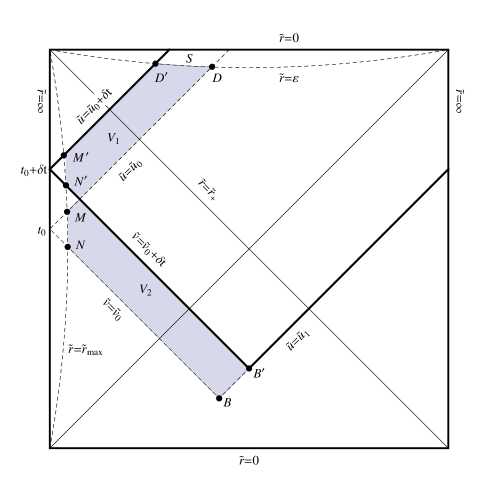
Figure 1: Wheeler-deWitt patches of a Schwarzschild-AdS black hole in $f\left(R\right)$ gravity at $\tilde{t}_{L}=t_{0}$ and $\tilde{t}_{L}=t_{0}+\delta t$. The lines $\tilde{r}=\tilde{r}_{\max}$ and $\tilde{r}=\varepsilon$ are the cut-off surfaces.

Due to time translation, the joint contributions from $\mathcal{D}$ and $\mathcal{D}^{\prime}$ are identical, and they therefore make no contribution to $\delta S_{\text{WdW}}$. Similarly, the joint and surface contributions from $\mathcal{MN}$ cancel against these from $\mathcal{M}^{\prime}\mathcal{N}^{\prime}$ on $\tilde{r}=\tilde{r}_{\max}$ in calculating $\delta S_{\text{WdW}}$. Since $S_{\partial\mathcal{V}}^{\phi}=0$ and null surfaces make no contribution to $\delta S_{\text{WdW}}$, eqn. $\left(\ref{eq:TotalS}\right)$ reduces to

$$\delta S_{\text{WdW}}=S_{\mathcal{V}_{1}}-S_{\mathcal{V}_{2}}+2\int_{\mathcal{S}}d^{d}\tilde{x}\sqrt{\left|\tilde{h}\right|}K+2\int_{\mathcal{B}^{\prime}}d^{d-1}\tilde{x}\sqrt{\tilde{\sigma}}a-2\int_{\mathcal{B}}d^{d-1}\tilde{x}\sqrt{\tilde{\sigma}}a.$$ (23)

Since the black hole solutions are on shell, the volume contribution can be calculated by eqn. $\left(\ref{eq:Sf(R)}\right)$

$$S_{\mathcal{V}} =f\left(R_{0}\right)\int_{\mathcal{V}}d^{d+1}x\sqrt{-g}=f\left(R_{0}\right)f^{\prime}\left(R_{0}\right)^{-\frac{d+1}{d-1}}\int_{\mathcal{V}}d^{d+1}\tilde{x}\sqrt{-\tilde{g}}$$

$$=f\left(R_{0}\right)f^{\prime}\left(R_{0}\right)^{-\frac{2d}{d-1}}\Omega_{k,d-1}\int_{\mathcal{V}}d\tilde{\omega}d\tilde{r}\tilde{r}^{d-1},$$ (24)

where $\tilde{\omega}=\left\{\tilde{t},\tilde{u},\tilde{v}\right\}$. The region $\mathcal{V}_{1}$ is bounded by the null surfaces $\tilde{u}=\tilde{u}_{0}$, $\tilde{u}=\tilde{u}_{0}+$ $\delta t$, $\tilde{v}=\tilde{v}_{0}+$ $\delta t$, the spacelike surface $\tilde{r}=\varepsilon$, and the timelike surface $\tilde{r}=\tilde{r}_{\max}$. Using eqn. $\left(\ref{eq:vc}\right)$, we have that

$$S_{\mathcal{V}_{1}} =f\left(R_{0}\right)f^{\prime}\left(R_{0}\right)^{-\frac{2d}{d-1}}\Omega_{k,d-1}\int_{\tilde{u}_{0}}^{\tilde{u}_{0}+\delta t}d\tilde{u}\int_{\varepsilon}^{\min\left\{\tilde{r}_{\max},\rho\left(\tilde{u}\right)\right\}}\tilde{r}^{d-1}d\tilde{r}$$

$$=\frac{f\left(R_{0}\right)f^{\prime}\left(R_{0}\right)^{-\frac{2d}{d-1}}\Omega_{k,d-1}}{d}\int_{\tilde{u}_{0}}^{\tilde{u}_{0}+\delta t}d\tilde{u}\tilde{r}^{d}|_{\tilde{r}=\min\left\{\tilde{r}_{\max},\rho\left(\tilde{u}\right)\right\}}\text{,}$$ (25)

where $\tilde{r}^{\ast}\left(\rho\left(\tilde{u}\right)\right)=\left(\tilde{v}_{0}+\delta t-\tilde{u}\right)/2$, and we neglect the $\varepsilon^{d-1}$ term. Similarly for $\mathcal{V}_{2}$, we find that

$$S_{\mathcal{V}2}=\frac{f\left(R_{0}\right)f^{\prime}\left(R_{0}\right)^{-\frac{2d}{d-1}}\Omega_{k,d-1}}{d}\int_{\tilde{v}_{0}}^{\tilde{v}_{0}+\delta t}d\tilde{v}\tilde{r}^{d}|_{\rho_{1}\left(\tilde{v}\right)}^{\min\left\{\tilde{r}_{\max},\rho_{0}\left(\tilde{v}\right)\right\}},$$ (26)

where $\tilde{r}^{\ast}\left(\rho_{0/1}\left(\tilde{v}\right)\right)=\left(\tilde{v}-\tilde{u}_{0/1}\right)/2$. Performing the change of variables $\tilde{u}=\tilde{u}_{0}+\tilde{v}_{0}+\delta t-\tilde{v}$, one has that

$$\int_{\tilde{v}_{0}}^{\tilde{v}_{0}+\delta t}d\tilde{v}\tilde{r}^{d}|_{\tilde{r}=\min\left\{\tilde{r}_{\max},\rho_{0}\left(\tilde{v}\right)\right\}}=\int_{\tilde{u}_{0}}^{\tilde{u}_{0}+\delta t}d\tilde{u}\tilde{r}^{d}|_{\tilde{r}=\min\left\{\tilde{r}_{\max},\rho\left(\tilde{u}\right)\right\}},$$ (27)

and hence

$$S_{\mathcal{V}_{1}}-S_{\mathcal{V}_{2}}=\frac{f\left(R_{0}\right)f^{\prime}\left(R_{0}\right)^{-\frac{2d}{d-1}}\Omega_{k,d-1}}{d}\int_{\tilde{v}_{0}}^{\tilde{v}_{0}+\delta t}d\tilde{v}\tilde{r}^{d}|_{r=\rho_{1}\left(\tilde{v}\right)},$$ (28)

which shows that the portion of $\mathcal{V}_{1}$ below the future horizon cancels against the portion of $\mathcal{V}_{2}$ above the past horizon. At late times, one has that $\rho_{1}\left(\tilde{v}\right)\approx\tilde{r}_{+}=f^{\prime}\left(R_{0}\right)^{\frac{2}{d-1}}r_{+}$, and

$$S_{\mathcal{V}_{1}}-S_{\mathcal{V}_{2}}=\frac{f\left(R_{0}\right)\Omega_{k,d-1}}{d}r_{+}^{d}\delta t\text{.}$$ (29)

There is a timelike hypersurface at $\tilde{r}=\varepsilon$, with outward-directed normal vectors from the region of interest. The normal vector is

$$\tilde{n}_{\mu}d\tilde{x}^{\mu}=\frac{-1}{\sqrt{-\tilde{b}\left(\tilde{r}\right)}}d\tilde{r}\text{.}$$ (30)

The trace of extrinsic curvature is

$$K=\frac{1}{\tilde{r}^{d-1}}\partial_{\tilde{r}}\left(\tilde{r}^{d-1}\sqrt{-\tilde{b}\left(\tilde{r}\right)}\right).$$ (31)

Therefore, the surface contributions from $\tilde{r}=\varepsilon$ is

$$2\int_{\mathcal{S}}d^{d}\tilde{x}\sqrt{\left|\tilde{h}\right|}K=mdf^{\prime}\left(R_{0}\right)\Omega_{k,d-1}\delta t,$$ (32)

where we use $\sqrt{\left|\tilde{h}\right|}=\sqrt{-\tilde{b}\left(\tilde{r}\right)}f^{\prime}\left(R_{0}\right)^{-1}\tilde{r}^{d-1}$ and $\tilde{b}\left(\tilde{r}\right)\sim-\frac{m}{\tilde{r}^{d-2}}f^{\prime}\left(R_{0}\right)^{2}$ for small $\tilde{r}$.

Following IN-Carmi:2016wjl , the integrand $a$ in the joint terms of eqn. $\left(\ref{eq:deltaSS}\right)$ is

$$a =\epsilon\ln\left|\mathbf{k}_{1}\cdot\mathbf{k}_{2}/2\right|,$$

$$\epsilon =-\text{sign}\left(\mathbf{k}_{1}\cdot\mathbf{k}_{2}\right)\text{sign}\left(\mathbf{\hat{k}}\cdot\mathbf{k}_{2}\right),$$ (33)

where for $\mathcal{B}$ and $\mathcal{B}^{\prime}$,

$$\left(\mathbf{k}_{1}\right)_{\mu} =-c_{1}\partial_{\tilde{\mu}}\left(\tilde{t}+\tilde{r}^{\ast}\right),$$

$$\left(\mathbf{k}_{2}\right)_{\mu} =c_{2}\partial_{\tilde{\mu}}\left(\tilde{t}-\tilde{r}^{\ast}\right),$$ (34)

and the auxiliary null vectors $\mathbf{\hat{k}}$ is the null vector orthogonal to the joint and pointing outward from the boundary region. Therefore, we find that

$$2\int_{\mathcal{B}^{\prime}}d^{d-1}\tilde{x}\sqrt{\tilde{\sigma}}a-2\int_{\mathcal{B}}d^{d-1}\tilde{x}\sqrt{\tilde{\sigma}}a=2\Omega_{k,d-1}\left[\tilde{h}\left(\tilde{r}_{\mathcal{B}^{\prime}}\right)-\tilde{h}\left(\tilde{r}_{\mathcal{B}}\right)\right],$$ (35)

where

$$\tilde{h}\left(\tilde{r}\right)=f^{\prime}\left(R_{0}\right)^{-1}\tilde{r}^{d-1}\ln\left(-\frac{\tilde{b}\left(\tilde{r}\right)}{c_{1}c_{2}}\right).$$ (36)

At late times, we have that $\tilde{r}_{\mathcal{B}}\approx\tilde{r}_{+}$ and

$$\tilde{h}\left(\tilde{r}_{\mathcal{B}^{\prime}}\right)-\tilde{h}\left(\tilde{r}_{\mathcal{B}}\right)=\frac{\tilde{b}\left(\tilde{r}\right)}{2}\frac{d\tilde{h}\left(\tilde{r}\right)}{d\tilde{r}}|_{\tilde{r}=\tilde{r}_{B}}\delta t=\frac{f^{\prime}\left(R_{0}\right)^{-1}\tilde{r}^{d-1}}{2}\frac{d\tilde{b}\left(\tilde{r}\right)}{d\tilde{r}}|_{\tilde{r}=\tilde{r}_{+}}\delta t,$$ (37)

where we use $d\tilde{r}=\tilde{b}\left(\tilde{r}\right)\delta t/2$ on $\tilde{u}=u_{1}$. Thus, this gives

$$2\int_{\mathcal{B}^{\prime}}d^{d-1}\tilde{x}\sqrt{\tilde{\sigma}}a-2\int_{\mathcal{B}}d^{d-1}\tilde{x}\sqrt{\tilde{\sigma}}a=\Omega_{k,d-1}f^{\prime}\left(R_{0}\right)r_{+}^{d-1}\left[\left(d-2\right)\frac{m}{r_{+}^{d-1}}+\frac{2r_{+}}{L^{2}}\right]\delta t,$$ (38)

where we use $d\tilde{b}\left(\tilde{r}\right)/d\tilde{r}=db\left(r\right)/dr$. Combining eqns. $\left(\ref{eq:S1}\right)$, $\left(\ref{eq:S2}\right)$, and $\left(\ref{eq:S3}\right)$, we arrive at

$$\delta S_{\text{WdW}}=2\left(d-1\right)f^{\prime}\left(R_{0}\right)\Omega_{d-1}m\delta t\text{,}$$ (39)

where we use eqn. $\left(\ref{eq:RT}\right)\,$ with $T^{m}=0$. Since $t=\tilde{t}$, eqn. $\left(\ref{eq:mass}\right)$ leads to

$$\frac{dS_{\text{WdW}}}{dt}=2M,$$ (40)

which has the same form as for the SAdS black hole in the Einstein’s gravity.

III.2 Charged Black Hole

To have a black hole solution with constant curvature, the trace of the energy-momentum tensor of the matter filed must vanish AGBHfG-Moon:2011hq . It is obvious that the standard Maxwell energy-momentum tensor is traceless in four dimensions but not in higher dimensions. On the other hand, an extension of Maxwell action in $\left(d+1\right)$-dimensional spacetime that is traceless is the conformally invariant Maxwell action AGBHfG-Hassaine:2007py :

$$S^{m}=-\int d^{d+1}x\sqrt{-g}\left(F_{\mu\nu}F^{\mu\nu}\right)^{\left(d+1\right)/4},$$ (41)

$F_{\mu\nu}=\partial_{\mu}A_{\nu}-\partial_{\nu}A_{\mu}$ is the electromagnetic field tensor, and $A_{\mu}$ is the electromagnetic potential. When $d=3$, the action $\left(\ref{eq:IMax}\right)$ recovers the standard Maxwell action. The EOM obtained by varying the action $\left(\ref{eq:action}\right)$ with respect to $A_{\mu}$ is

$$\partial_{\mu}\left(\sqrt{-g}F^{\mu\nu}F^{\left(d-1\right)/4}\right)=0,$$ (42)

where $F=F^{\mu\nu}F_{\mu\nu}$. Together with the gravitational equation $\left(\ref{eq:RT}\right)$, the black hole solution was given in AGBHfG-Sheykhi:2012zz :

$$ds^{2} =-b\left(r\right)dt^{2}+\frac{dr^{2}}{b\left(r\right)}+r^{2}d\Sigma_{k,d-1}^{2},$$

$$F_{tr} =\frac{q}{r^{2}},$$ (43)

where

$$b\left(r\right)=k-\frac{m}{r^{d-2}}+\frac{q^{2}}{r^{d-1}}\frac{\left(-2q^{2}\right)^{\left(d-3\right)/4}}{f^{\prime}\left(R_{0}\right)}+\frac{r^{2}}{L^{2}},$$ (44)

and the constant Ricci scalar $R_{0}\equiv-\frac{\left(d+1\right)d}{L^{2}}$. To have a real solution, the dimensions $d+1$ must be multiples of four, i.e., $d=3,7,\cdots$. The parameters $m$ and $q$ are related to the mass $M$ and charge $Q$ of the black hole by AGBHfG-Sheykhi:2012zz

$$M =f^{\prime}\left(R_{0}\right)\left(d-1\right)\Omega_{k,d-1}m,$$

$$Q =\frac{\left(d+1\right)\left(-2\right)^{\left(d-3\right)/4}q^{\left(d-1\right)/2}\Omega_{k,d-1}}{16\pi\sqrt{f^{\prime}\left(R_{0}\right)}},$$ (45)

and the electric potential $\Phi$ at the horizon radius $r_{\pm}$ is

$$\Phi_{\pm}=16\pi\frac{q}{r_{\pm}}\sqrt{f^{\prime}\left(R_{0}\right)}.$$ (46)

As argued before, one has $f^{\prime}\left(R_{0}\right)>0$ to obtain physical solutions. The black hole solution $\left(\ref{eq:CBH}\right)$ is similar to a Reissner-Nordstrom AdS black hole. Thus, this solution could have two horizons at the outer radius $r_{+}$ and inner radius $r_{-}$, respectively. When $r_{+}=r_{-}$, the black hole is extremal.

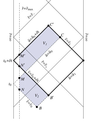
Figure 2: Wheeler-deWitt patches of a charged black hole in $f\left(R\right)$ gravitiy at $\tilde{t}_{L}=t_{0}$ and $\tilde{t}_{L}=t_{0}+\delta t$. The line $\tilde{r}=\tilde{r}_{\max}$ is the cut-off surface.

We now calculate the change $\delta S_{\text{WdW}}=S_{\text{WdW}}\left(t_{0}+\delta t\right)-$ $S_{\text{WdW}}\left(t_{0}\right)$ in the total action $\left(\ref{eq:TotalS}\right)$ between the two WdW patches displayed in FIG. 2. Taking time translation into account, $\delta S_{\text{WdW}}$ reduces to

$$\delta S_{\text{WdW}}=S_{\mathcal{V}_{1}}-S_{\mathcal{V}_{2}}+2\int_{\mathcal{B}^{\prime}}d^{d-1}\tilde{x}\sqrt{\tilde{\sigma}}a-2\int_{\mathcal{B}}d^{d-1}\tilde{x}\sqrt{\tilde{\sigma}}a+2\int_{\mathcal{C}^{\prime}}d^{d-1}\tilde{x}\sqrt{\tilde{\sigma}}a-2\int_{\mathcal{C}}d^{d-1}\tilde{x}\sqrt{\tilde{\sigma}}a.$$ (47)

For the black hole solution $\left(\ref{eq:CBH}\right)$, we find that the volume contribution is

$$S_{\mathcal{V}}=\Omega_{k,d-1}\int_{\mathcal{V}}d\tilde{\omega}F\left(\tilde{r}\right),$$ (48)

where $\tilde{\omega}=\left\{\tilde{u},\tilde{v}\right\}$, and

$$F\left(\tilde{r}\right)=-\frac{2f^{\prime}\left(R_{0}\right)}{L^{2}}\tilde{r}^{d}+f^{\prime}\left(R_{0}\right)^{\frac{2\left(d+1\right)}{d-1}}\frac{\left(-2q^{2}\right)^{\left(d+1\right)/4}}{\tilde{r}}\text{.}$$ (49)

For $\mathcal{V}_{1}$, its volume contribution is

$$S_{\mathcal{V}_{1}}=f^{\prime}\left(R_{0}\right)^{-\frac{2}{d-1}}\Omega_{k,d-1}\int_{\tilde{u}_{0}}^{\tilde{u}_{0}+\delta t}d\tilde{u}F\left(\tilde{r}\right)|_{\tilde{\rho}_{1}\left(\tilde{u}\right)}^{\min\left\{\tilde{r}_{\max},\rho\left(\tilde{u}\right)\right\}}d\tilde{r},$$ (50)

where $\tilde{r}^{\ast}\left(\rho\left(\tilde{u}\right)\right)=\left(\tilde{v}_{0}+\delta t-\tilde{u}\right)/2$ and $r^{\ast}\left(\tilde{\rho}_{1}\left(\tilde{u}\right)\right)=\frac{\tilde{v}_{1}-\tilde{u}}{2}$. Similarly, the volume contribution $S_{\mathcal{V}_{2}}\,$is

$$S_{\mathcal{V}2}=f^{\prime}\left(R_{0}\right)^{-\frac{2}{d-1}}\Omega_{k,d-1}\int_{\tilde{v}_{0}}^{\tilde{v}_{0}+\delta t}d\tilde{v}F\left(\tilde{r}\right)|_{\rho_{1}\left(\tilde{v}\right)}^{\min\left\{\tilde{r}_{\max},\rho_{0}\left(\tilde{v}\right)\right\}},$$ (51)

where $r^{\ast}\left(\rho_{0/1}\left(\tilde{v}\right)\right)=\left(\tilde{v}-\tilde{u}_{0/1}\right)/2$. Making the change of variables $\tilde{u}=\tilde{u}_{0}+\tilde{v}_{0}+\delta t-\tilde{v}$, we find that at late times,

$$\delta S_{\mathcal{V}} =f^{\prime}\left(R_{0}\right)^{-\frac{2}{d-1}}\Omega_{k,d-1}\left[\int_{\tilde{v}_{0}}^{\tilde{v}_{0}+\delta t}d\tilde{v}F\left(\tilde{r}\right)|_{r=\rho_{1}\left(v\right)}-\int_{\tilde{u}_{0}}^{\tilde{u}_{0}+\delta t}d\tilde{u}F\left(\tilde{r}\right)|_{r=\tilde{\rho}_{1}\left(\tilde{u}\right)}d\tilde{r}\right]$$

$$=\Omega_{k,d-1}\left[-\frac{2f^{\prime}\left(R_{0}\right)}{L^{2}}r^{d}+\frac{\left(-2q^{2}\right)^{\left(d+1\right)/4}}{r}\right]|_{r_{-}}^{r_{+}}\delta t,$$ (52)

where $r_{+}\,$and $r_{-}$ are the outer and inner horizon radius, respectively.

For the joint contributions from $\mathcal{B}$ and $\mathcal{B}^{\prime}$ at late times, eqns. $\left(\ref{eq:2sigma}\right)$ and $\left(\ref{eq:h}\right)$ give

$$2\int_{\mathcal{B}^{\prime}}d^{d-1}\tilde{x}\sqrt{\tilde{\sigma}}a-2\int_{\mathcal{B}}d^{d-1}\tilde{x}\sqrt{\tilde{\sigma}}a=\Omega_{k,d-1}f^{\prime}\left(R_{0}\right)^{-1}\tilde{r}^{d-1}\frac{d\tilde{b}\left(\tilde{r}\right)}{d\tilde{r}}|_{\tilde{r}=\tilde{r}_{+}}\delta t$$

$$=\Omega_{k,d-1}f^{\prime}\left(R_{0}\right)\left[\left(d-2\right)m-\frac{\left(d-1\right)q^{2}}{r_{+}}\frac{\left(-2q^{2}\right)^{\left(d-3\right)/4}}{f^{\prime}\left(R_{0}\right)}+\frac{2r_{+}^{d}}{L^{2}}\right]\delta t.$$ (53)

Analogously to deriving eqn. $\left(\ref{eq:SBB}\right)$, we find that

$$2\int_{\mathcal{C}^{\prime}}d^{d-1}\tilde{x}\sqrt{\tilde{\sigma}}a-2\int_{\mathcal{C}}d^{d-1}\tilde{x}\sqrt{\tilde{\sigma}}a=-\Omega_{k,d-1}f^{\prime}\left(R_{0}\right)\left[\left(d-2\right)m-\frac{\left(d-1\right)q^{2}}{r_{-}}\frac{\left(-2q^{2}\right)^{\left(d-3\right)/4}}{f^{\prime}\left(R_{0}\right)}+\frac{2r_{-}^{d}}{L^{2}}\right]\delta t.$$ (54)

Summing up all the contributions, we obtain

$$\delta S_{\text{WdW}}=\Omega_{k,d-1}\left(d+1\right)\frac{\left(-2\right)^{\left(d-3\right)/4}q^{\left(d+1\right)/2}}{r}|_{r_{+}}^{r-}\delta t.$$ (55)

Using eqns. $\left(\ref{eq:MQ}\right)$ and $\left(\ref{eq:Phi}\right)$, we can write $dS/dt$ in terms of $Q$ and $\Phi_{\pm}$:

$$\frac{dS_{\text{WdW}}}{dt}=Q\Phi_{-}-Q\Phi_{+}.$$ (56)

IV Discussion and Conclusion

In this paper, we used the approach proposed by Lehner et al. IN-Lehner:2016vdi to calculate the change of the action of Wheeler-DeWitt patches in $f\left(R\right)$ gravity. However, the method proposed in IN-Lehner:2016vdi only works for the Einstein–Hilbert action. In section II, we instead considered a (classically) dynamically equivalent theory of $f\left(R\right)$ gravity, which was a Brans-Dicke theory with Brans–Dicke parameter $\omega_{\text{BD}}=0$. After transforming the Brans–Dicke action in the Jordan frame to the Einstein frame by a conformal transformation, we showed that the action in Einstein frame was the Einstein-Hilbert action plus the actions of the matter field and an auxiliary field. In section III, the black hole solutions in $f\left(R\right)$ gravity with constant curvature were discussed in the cases of the vacuum and power-Maxwell field, respectively. In vacuum, the black hole solution was a Schwarzschild-AdS black hole. Coupled to a conformally invariant Maxwell field, the black hole solution was similar to a higher dimensional Reissner-Nordstrom AdS black hole but only exist for dimensions which are multiples of four. The results for the rate of the action at late times are summarized as

Schwarzschild-AdS black hole $$\text{: }\frac{dS_{\text{WdW}}}{dt}=2M,$$

Charged black hole $$\text{: }\frac{dS_{\text{WdW}}}{dt}=Q\Phi_{-}-Q\Phi_{+},$$ (57)

where $M$ and $Q$ are the mass and charge of the black hole, respectively; $\Phi_{\pm}$ are the electric potential evaluated at $r_{\pm}$, respectively. It is noteworthy that these results in $f\left(R\right)$ gravity have the same form as in Einstein’s gravity.

Currently, there are two approaches to calculate the action of Wheeler-DeWitt patches. In IN-Lehner:2016vdi , contributions from null surfaces were zero by choosing affine parameterizations while contributions from joints were considered. On the other hand, no contributions from joints were considered in IN-Brown:2015lvg . However, contributions from spacelike/timelike surface approaching the null surface were included there. Although these two approaches seem quite different, it showed IN-Lehner:2016vdi that they yielded the same results for various black holes in Einstein’s gravity. The $dS_{\text{WdW}}/dt$ for a Schwarzschild-AdS black hole in $f\left(R\right)$ gravity was calculated in IN-Alishahiha:2017hwg using the method of IN-Brown:2015lvg , and the result in IN-Alishahiha:2017hwg is the same as in our paper. It seems that both approaches may give the same result in $f\left(R\right)$ gravity. Whether there is a reason for this coincidence deserves further considerations.

In IN-Cai:2016xho , the action growth of the Wheeler-DeWitt patches in the cases of AdS-RN black holes, (charged) rotating BTZ black holes, AdS Kerr black holes and (charged) Gauss-Bonnet black holes were calculated using the method of IN-Brown:2015lvg . It was found there that the results could be written as

$$\frac{dS_{\text{WdW}}}{dt}=\left(M-\Omega J-Q\Phi\right)_{+}-\left(M-\Omega J-Q\Phi\right)_{-},$$ (58)

where $\Omega$ and $\Phi$ are angular velocity and electrical potential of a black hole, respectively; $J$ and $Q$ are the angular momentum and electric charge of the black hole, respectively; the subscript $+/-$ stand for evaluations at the outer and inner horizons, respectively. The same expression for the results in IN-Pan:2016ecg was also obtained in the case of massive gravities. A general case was considered in CON-Huang:2016fks , and it was proved that the action growth rate equals the difference of the generalized enthalpy at the outer and inner horizons. In our paper, we showed that the action growth for charged black holes in $f\left(R\right)$ gravity could also be rewritten as form of eqn. $\left(\ref{eq:ds/dtC}\right)$.

The Lloyd bound CON-Llo:2000 on the complexity growth for a holographic state dual to a uncharged black hole reads IN-Brown:2015lvg

$$\mathcal{\dot{C}\leq}\frac{2M}{\pi\hbar},$$ (59)

where $M$ is the mass of the black hole. We showed that by CA duality $\left(\ref{eq:CA}\right)$, the complexity growth for a Schwarzschild-AdS black hole black hole in $f\left(R\right)$ gravity saturates the Lloyd bound $\left(\ref{eq:LN}\right)$. It has been proved in CON-Yang:2016awy that under the strong energy condition of steady matter outside the Killing horizon, black holes in CA duality obey the Lloyd bound. As noted in IN-Brown:2015lvg , the rate of the complexity of a neutral black hole is faster than that of a charged black hole due to the existence of conserved charges. This leads to that the Lloyd bound can be generalized for a charged black hole with the charge $Q$:

$$\mathcal{\dot{C}\leq}\frac{2}{\pi\hbar}\left[\left(M-Q\Phi\right)_{+}-\left(M-Q\Phi\right)_{\text{gs}}\right],$$ (60)

where $\Phi$ is the potential at the horizon, and $\left(M-Q\Phi\right)_{+/\text{gs}}$ are $M-Q\Phi$ calculated at the outer horizon and in the ground state, respectively. Treating the system as a grand canonical ensemble implies that the ground state has the same potential as the black hole under consideration. For charged black holes in $f\left(R\right)$ gravity, the ground states are extremal black holes with $r_{+}=r_{-}$. Near extremality, our previous paper IN-Tao:2017fsy showed that the Lloyd bound $\left(\ref{eq:LBoundQ}\right)$ is usually violated for charged black holes. These violations may have something to do with hair IN-Brown:2015lvg .

For charged black holes $\left(\ref{eq:CBH}\right)$ with fixed potential $\Phi_{+}=\Phi_{0}$ far away from the ground state, one has large black holes with $r_{+}\gg L$. In this case, we find that

$$2\left(M-Q\Phi\right)_{+}-2\left(M-Q\Phi\right)_{\text{gs}}=2f^{\prime}\left(R_{0}\right)\left(d-1\right)\Omega_{k,d-1}\frac{r_{+}^{d}}{L^{2}}\left[1+\mathcal{O}\left(\frac{L^{2}}{r_{+}^{2}}\right)\right],$$ (61)

$$\frac{dS_{\text{WdW}}}{dt}=Q\Phi_{-}-Q\Phi_{+}=f^{\prime}\left(R_{0}\right)\Omega_{k,d-1}\frac{\left(d+1\right)r_{+}^{d}}{L^{2}}\left[1+\mathcal{O}\left(\frac{L^{2}}{r_{+}^{2}}\right)\right],$$

which show that the Lloyd bound is satisfied but not saturated for charged black holes with $d=7,11,\cdots$. However for $d=3$, we need to find higher order terms to check whether the Lloyd bound is violated. When $d=3$, we obtain

$$2\left(M-Q\Phi\right)_{+}-2\left(M-Q\Phi\right)_{\text{gs}}=16\pi f^{\prime}\left(R_{0}\right)\frac{r_{+}^{3}}{L^{2}}\left[1+\frac{kL^{2}}{r_{+}^{2}}-\frac{1}{f^{\prime}\left(R_{0}\right)^{2}}\left(\frac{\Phi_{0}}{16\pi}\right)^{4}\frac{L^{2}}{r_{+}^{2}}+\mathcal{O}\left(\frac{L^{3}}{r_{+}^{3}}\right)\right],$$ (62)

$$\frac{dS_{\text{WdW}}}{dt}=Q\Phi_{-}-Q\Phi_{+}=16\pi f^{\prime}\left(R_{0}\right)\frac{r_{+}^{3}}{L^{2}}\left[1+\frac{kL^{2}}{r_{+}^{2}}+\mathcal{O}\left(\frac{L^{4}}{r_{+}^{4}}\right)\right],$$

which shows that the Lloyd bound is violated.

- (1) A. R. Brown, D. A. Roberts, L. Susskind, B. Swingle and Y. Zhao, “Holographic Complexity Equals Bulk Action?,” Phys. Rev. Lett. 116, no. 19, 191301 (2016) doi:10.1103/PhysRevLett.116.191301 [arXiv:1509.07876 [hep-th]].
- (2) A. R. Brown, D. A. Roberts, L. Susskind, B. Swingle and Y. Zhao, “Complexity, action, and black holes,” Phys. Rev. D 93, no. 8, 086006 (2016) doi:10.1103/PhysRevD.93.086006 [arXiv:1512.04993 [hep-th]].
- (3) J. Watrous, “Quantum computational complexity,” in Encyclopedia of Complexity and Systems Science, ed., R. A. Meyers (2009) 7174–7201, arXiv:0804.3401 [quant-ph].
- (4) S. Gharibian, Y. Huang, Z. Landau, and S. W. Shin, “Quantum hamiltonian complexity,” Foundations and Trends in Theoretical Computer Science 10 (2015) 159–282, arXiv:1401.3916 [quant-ph].
- (5) T. J. Osborne, “Hamiltonian complexity,” Reports on Progress in Physics 75 (2012) 022001, arXiv:1106.5875 [quant-ph].
- (6) L. Susskind, “Computational Complexity and Black Hole Horizons,” Fortsch. Phys. 64, 24 (2016) doi:10.1002/prop.201500092 [arXiv:1403.5695 [hep-th], arXiv:1402.5674 [hep-th]].
- (7) D. Stanford and L. Susskind, “Complexity and Shock Wave Geometries,” Phys. Rev. D 90, no. 12, 126007 (2014) doi:10.1103/PhysRevD.90.126007 [arXiv:1406.2678 [hep-th]].
- (8) L. Susskind and Y. Zhao, “Switchbacks and the Bridge to Nowhere,” arXiv:1408.2823 [hep-th].
- (9) L. Susskind, “Entanglement is not enough,” Fortsch. Phys. 64, 49 (2016) doi:10.1002/prop.201500095 [arXiv:1411.0690 [hep-th]].
- (10) J. Couch, W. Fischler and P. H. Nguyen, “Noether Charge, Black Hole Volume, and Complexity,” arXiv:1610.02038 [hep-th].
- (11) L. Lehner, R. C. Myers, E. Poisson and R. D. Sorkin, “Gravitational action with null boundaries,” Phys. Rev. D 94, no. 8, 084046 (2016) doi:10.1103/PhysRevD.94.084046 [arXiv:1609.00207 [hep-th]].
- (12) R. G. Cai, S. M. Ruan, S. J. Wang, R. Q. Yang and R. H. Peng, “Action growth for AdS black holes,” JHEP 1609, 161 (2016) doi:10.1007/JHEP09(2016)161 [arXiv:1606.08307 [gr-qc]].
- (13) W. J. Pan and Y. C. Huang, “Holographic complexity and action growth in massive gravities,” arXiv:1612.03627 [hep-th].
- (14) M. Alishahiha, A. Faraji Astaneh, A. Naseh and M. H. Vahidinia, “On Complexity for Higher Derivative Gravities,” arXiv:1702.06796 [hep-th].
- (15) R. G. Cai, M. Sasaki and S. J. Wang, “Action growth of charged black holes with a single horizon,” arXiv:1702.06766 [gr-qc].
- (16) J. Tao, P. Wang and H. Yang, “Testing Holographic Conjectures of Complexity with Born-Infeld Black Holes,” arXiv:1703.06297 [hep-th].
- (17) D. Carmi, R. C. Myers and P. Rath, “Comments on Holographic Complexity,” arXiv:1612.00433 [hep-th].
- (18) A. Reynolds and S. F. Ross, “Divergences in Holographic Complexity,” arXiv:1612.05439 [hep-th].
- (19) K. Y. Kim, C. Niu and R. Q. Yang, “Surface Counterterms and Regularized Holographic Complexity,” arXiv:1701.03706 [hep-th].
- (20) P. G. Bergmann, “Comments on the scalar tensor theory,” Int. J. Theor. Phys. 1, 25 (1968). doi:10.1007/BF00668828
- (21) S. Capozziello, M. De Laurentis and V. Faraoni, “A Bird’s eye view of f(R)-gravity,” Open Astron. J. 3, 49 (2010) doi:10.2174/1874381101003010049, 10.2174/1874381101003020049 [arXiv:0909.4672 [gr-qc]].
- (22) S. Capozziello and M. De Laurentis, “Extended Theories of Gravity,” Phys. Rept. 509, 167 (2011) doi:10.1016/j.physrep.2011.09.003 [arXiv:1108.6266 [gr-qc]].
- (23) S. Nojiri and S. D. Odintsov, “Unified cosmic history in modified gravity: from F(R) theory to Lorentz non-invariant models,” Phys. Rept. 505, 59 (2011) doi:10.1016/j.physrep.2011.04.001 [arXiv:1011.0544 [gr-qc]].
- (24) A. De Felice and S. Tsujikawa, “f(R) theories,” Living Rev. Rel. 13, 3 (2010) doi:10.12942/lrr-2010-3 [arXiv:1002.4928 [gr-qc]].
- (25) T. Moon, Y. S. Myung and E. J. Son, “f(R) black holes,” Gen. Rel. Grav. 43, 3079 (2011) doi:10.1007/s10714-011-1225-3 [arXiv:1101.1153 [gr-qc]].
- (26) A. de la Cruz-Dombriz, A. Dobado and A. L. Maroto, “Black Holes in f(R) theories,” Phys. Rev. D 80, 124011 (2009) Erratum: [Phys. Rev. D 83, 029903 (2011)] doi:10.1103/PhysRevD.83.029903, 10.1103/PhysRevD.80.124011 [arXiv:0907.3872 [gr-qc]].
- (27) L. Pogosian and A. Silvestri, “The pattern of growth in viable f(R) cosmologies,” Phys. Rev. D 77, 023503 (2008) Erratum: [Phys. Rev. D 81, 049901 (2010)] doi:10.1103/PhysRevD.77.023503, 10.1103/PhysRevD.81.049901 [arXiv:0709.0296 [astro-ph]].
- (28) M. Hassaine and C. Martinez, “Higher-dimensional black holes with a conformally invariant Maxwell source,” Phys. Rev. D 75, 027502 (2007) doi:10.1103/PhysRevD.75.027502 [hep-th/0701058].
- (29) A. Sheykhi, “Higher-dimensional charged black holes,” Phys. Rev. D 86, 024013 (2012) doi:10.1103/PhysRevD.86.024013 [arXiv:1209.2960 [hep-th]].
- (30) R. Q. Yang, “Strong energy condition and the fastest computers,” arXiv:1610.05090 [gr-qc].
- (31) H. Huang, X. H. Feng and H. Lu, “Holographic Complexity and Two Identities of Action Growth,” arXiv:1611.02321 [hep-th].
- (32) S. Lloyd, “Ultimate physical limits to computation,” Nature 406 (2000), no. 6799 10471054.