Flavour Anomalies in $b\rightarrow s\ell^{+}\ell^{-}$ Processes -
a round table Discussion

Abstract

Precision measurements of flavour observables provide powerful tests of many extensions of the Standard Model. This contribution covers a range of flavour measurements of $b\rightarrow s\ell^{+}\ell^{-}$ transitions, several of which are in tension with the Standard Model of particle physics, as well as their theoretical interpretation. The basics of the theoretical background are discussed before turning to the main question of the field: whether the anomalies can be explained by QCD effects or whether they may be indicators of effects beyond the Standard Model.

1 Introduction

Flavour physics has a long track record of discoveries that paved the way for advances in particle physics. In particular the discovery of the ${B}^{0}$ meson oscillations in 1987 Prentice:1987ap is a great example demonstrating the potential of flavour physics to infer physics of high mass scales through precision measurements at low scales: the observed rate of oscillations was the first indication of the top quark being much heavier than the other five quark flavours. Precision flavour measurements at the LHC are sensitive to indirect effects from physics beyond the Standard Model (SM) at far greater scales than those accessible in direct searches.

This paper summarises a panel discussion focussing on a range of anomalies seen in measurements of ${b}\!\rightarrow{s}\ell^{+}\ell^{-}$ decays, which are a sensitive class of processes to potential effects beyond the SM (BSM). The central question is whether the observed anomalies are indeed BSM effects or whether they can be explained by QCD effects. The general ${b}\!\rightarrow{s}\ell^{+}\ell^{-}$ framework is briefly discussed below, the experimental situation is reviewed in Sec. 2, which are followed by theory Secs. 3-5 on the heavy quark framework, form-factor determinations and the relevance of long distance charm contributions. Global fit strategies aiming to combine experimental observables to extract a more precise theoretical picture are presented in Sec. 6, and finally Sec. 7 covers potential BSM interpretations of the flavour anomalies before the summary, which is given in Sec. 8.

1.1 General ${b}\!\rightarrow{s}\ell^{+}\ell^{-}$ framework

In order to maintain some coherence between the different contributions of various authors we give the effective Hamiltonian with some minimal explanation referencing to the theory based sections.

$$\mathcal{H}_{\mathrm{eff}}=\frac{G_{F}}{\sqrt{2}}\left(\sum_{i=1}^{2}(\lambda_{u}C_{i}O_{i}^{u}+\lambda_{c}C_{i}\mathcal{O}_{i}^{c})-\lambda_{t}\sum_{i=3}^{10}C_{i}O_{i}\right)\;,\qquad\lambda_{i}\equiv V_{\text{is}}^{*}V_{\text{ib}}\;,$$ (1)

where $V_{\text{ij}}$ are CKM-elements, $\mu$ is a factorisation scale, $C_{i}$ the Wilson coefficients encoding the ultraviolet (UV) physics and some of the most important operators are

$$\mathcal{O}_{1}^{q} \;=\; (\bar{s}_{i}q_{j})_{V-A}(\bar{q}_{j}b_{i})_{V-A}\;,\qquad\qquad \mathcal{O}_{2}^{q} \;=\; (\bar{s}_{i}q_{i})_{V-A}(\bar{q}_{j}b_{j})_{V-A}\;,$$

$$\mathcal{O}_{7[8]} \;=\; -\frac{em_{b}}{8\pi^{2}}\bar{s}\sigma\cdot F[G](1+\gamma_{5})b\;, \mathcal{O}_{9,10} \;=\; \frac{\alpha}{2\pi}(\bar{\ell}\gamma^{\mu}[\gamma_{5}]\ell)(\bar{s}\gamma_{\mu}(1-\gamma_{5})b)\;,$$ (2)

where $i,j$ are colour indices, $(\bar{s}b)_{V\pm A}=\bar{s}\gamma^{\mu}(1\pm\gamma_{5})b$, $e=\sqrt{4\pi\alpha}>0$ and $G_{F}$ is the Fermi constant. The Wilson coefficients $C_{i}$ are computed to next-to-next-to-leading order (NNLO) in perturbation theory, and the matrix elements of the operators are of non-perturbative nature. Those are either local short distance form-factors or non-local long distance matrix elements. The form-factors are computed in LCSR and in lattice QCD in complementary regimes as discussed in Sec. 4, and obey some symmetry relations for large large $m_{b}$-mass, cf. Secs 3 and 4.3 respectively. At large recoil of the lepton pair the matrix elements are evaluated outside the resonance region, either within the heavy quark expansion or LCSR as discussed in Secs. 3 and 5 respectively. At low-recoil an OPE has been proposed cf. Sec. 3, subject to potentially significant corrections from resonant charm contribution as discussed in Sec. 5.

2 Summary of experimental situation (T. Blake)

There has been huge experimental progress in measurements of rare $b\rightarrow s$ processes in the past five years. This has been driven by the large ${b}{\overline{b}}$ production cross-section in $pp$ collisions at the LHC, which enabled the LHC experiments to collect unprecedented samples of decays with dimuon final-states.

2.1 Leptonic decays

The decay ${{B}^{0}_{s}}\!\rightarrow{\mu^{+}\mu^{-}}$ is considered a golden mode for testing the SM at the LHC. The SM branching fraction depends on a single hadronic parameter, the ${B}^{0}_{s}$ decay constant, that be computed from Lattice CQD. Consequently the SM branching fraction is known to better than a 10% precision Bobeth:2013uxa . A combined analysis of the CMS and LHCb datasets LHCb-PAPER-2014-049 results in a time-averaged measurement of the branching fraction of the decay of

$$\overline{{\mathcal{B}}}({{B}^{0}_{s}}\!\rightarrow{\mu^{+}\mu^{-}})=(2.8^{+0.7}_{-0.6})\times 10^{-9}\leavevmode\nobreak\ .$$ (3)

A recent ATLAS measurement Aaboud:2016ire yields

$$\overline{{\mathcal{B}}}({{B}^{0}_{s}}\!\rightarrow{\mu^{+}\mu^{-}})=(0.9^{+1.1}_{-0.8})\times 10^{-9}\leavevmode\nobreak\ ,$$ (4)

which is consistent with the combined analysis from CMS and LHCb. These measurements are in good agreement with SM predictions and set strong constraints on extensions of the SM that introduce new scalar or pseudoscalar couplings.

2.2 Semileptonic decays

The large dataset has also enabled the LHCb and CMS experiments to make the most precise measurements of the differential branching fraction of ${B}\!\rightarrow K^{(*)}{\mu^{+}\mu^{-}}$ and ${{B}^{0}_{s}}\!\rightarrow\phi{\mu^{+}\mu^{-}}$ to date LHCb-PAPER-2014-006 ; LHCb-PAPER-2015-023 ; Khachatryan:2015isa . Above the open charm threshold, broad resonances are seen in the LHCb dataset LHCb-PAPER-2013-039 . The most prominent of these is the $\psi(4160)$. The regions close to the narrow charmonium resonances are excluded from the analysis. With the present binning scheme, the uncertainties on differential branching fraction measurements are limited by the knowledge of the ${B}\!\rightarrow{{J\mskip-3.0mu/\mskip-2.0mu\psi\mskip 2.0mu}}K^{(*)}$ and ${{B}^{0}_{s}}\!\rightarrow{{J\mskip-3.0mu/\mskip-2.0mu\psi\mskip 2.0mu}}\phi$ branching fractions that are used to normalise the signal. The measured differential branching fractions of $b\rightarrow s{\mu^{+}\mu^{-}}$ processes, tend to prefer smaller values than their corresponding SM predictions. The largest discrepancy is seen in the ${{B}^{0}_{s}}\!\rightarrow\phi{\mu^{+}\mu^{-}}$ decay, where the data are more than $3\,\sigma$ from the SM predictions in the dimuon invariant mass squared range $1<{q^{2}}<6\mathrm{\,Ge\kern-1.00006ptV}^{2}/c^{4}$, see Fig 1.

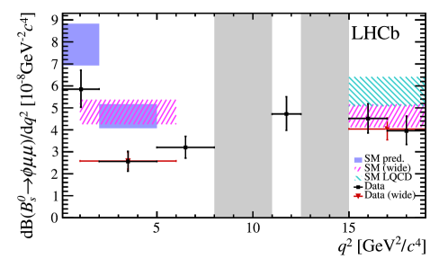
Figure 1: Differential branching fraction of the ${{B}^{0}_{s}}\!\rightarrow\phi{\mu^{+}\mu^{-}}$ decay measured by the LHCb experiment LHCb-PAPER-2015-023 as a function of the dimuon invariant mass squared, $q^{2}$. The data are compared to SM predictions based on Refs. Altmannshofer:2014rta ; Straub:2015ica and Horgan:2013pva . The rise in the branching fraction at low $q^{2}$ arises from virtual photon contributions to the decay. Reproduced from Ref. LHCb-PAPER-2015-023 .

While the branching fractions of rare $B\!\rightarrow K^{(*)}{\mu^{+}\mu^{-}}$ decays have large theoretical uncertainties arising from the ${B}\rightarrow K^{(*)}$ form-factors, many sources of uncertainty will cancel when comparing the decay rates of the $B\!\rightarrow K^{(*)}{\mu^{+}\mu^{-}}$ and $B\!\rightarrow K^{(*)}{e^{+}}{e^{-}}$ decays. In the range $1<q^{2}<6\mathrm{\,Ge\kern-1.00006ptV}^{2}/c^{4}$, the LHCb experiment measures LHCb-PAPER-2014-024

$$R_{K}[1,6]=0.745\,^{+0.090}_{-0.074}({\rm stat})\,^{+0.035}_{-0.035}({\rm syst})\,.$$ (5)

This is approximately $2.6\,\sigma$ from the SM expectation of almost identical decay rates for the two channels. In order to cancel systematic differences between the reconstruction of electrons and muons in the detector, the LHCb analysis is performed as a double ratio to the rate ${{{B}^{+}}}\!\rightarrow{{J\mskip-3.0mu/\mskip-2.0mu\psi\mskip 2.0mu}}{{K}^{+}}$ decays (where the ${J\mskip-3.0mu/\mskip-2.0mu\psi\mskip 2.0mu}$ can decay to a dielectron or dimuon pair). The migration of events in $q^{2}$ due to final-state-radiation is accounted for using samples of simulated events. QED effects are simulated through PHOTOS Golonka:2005pn . The largest difference between the dimuon and dielectron final-states comes from Bremsstrahlung from the electrons in the detector. This is simulated using GEANT 4 Agostinelli:2002hh . The modelling of the migration of events and the line-shape of the decay are the main contributions to the systematic uncertainty on the measurement.

The distribution of the final-state particles in the $B\!\rightarrow{{K}^{*}}\ell^{+}\ell^{-}$ decay can be described by three angles and $q^{2}$. The angles are: the angle between the direction of the $\ell^{+}$ ($\ell^{-}$) and the $B$ ($\kern 1.79993pt\overline{\kern-1.79993ptB}{}$) in the rest-frame of the dilepton pair; the angle between the direction of the kaon and the direction of the $B$ in the ${K}^{*}$ rest-frame; and the angle between the decay planes of the dilepton pair and the ${K}^{*}$ in the rest-frame of the $B$, denoted $\phi$. The resulting angular distribution can be parameterised in terms of eight angular observables: the longitudinal polarisation of the ${K}^{*}$, $F_{\rm L}$; the forward-backward asymmetry of the dilepton system, $A_{\rm FB}$; and six additional observables that cancel when integrating over $\phi$. Existing measurements of the observables $A_{\rm FB}$ and $F_{\rm L}$ are shown in Fig. 2 along with SM predictions based on Refs. Altmannshofer:2014rta ; Straub:2015ica . The most precise measurements of the $F_{\rm L}$ and $A_{\rm FB}$ come from the LHCb and CMS experiments. In general, the measurements are consistent with each other and are compatible with the SM predictions. The largest tension is seen in the BaBar measurement of $F_{\rm L}$ Lees:2015ymt .

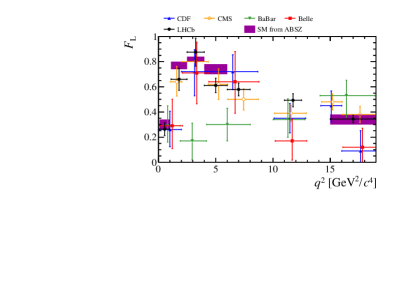
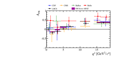
Figure 2: Observables $F_{\rm L}$ and $A_{\rm FB}$ measured by the BaBar Lees:2015ymt , Belle Wei:2009zv , CDF Aaltonen:2011ja , CMS Khachatryan:2015isa and LHCb LHCb-PAPER-2015-051 experiments for the $B\!\rightarrow{{K}^{*}}{\mu^{+}\mu^{-}}$ decay as a function of the dimuon invariant mass squared, $q^{2}$. The shaded region indicates a theoretical prediction for the observables based on Refs. Altmannshofer:2014rta ; Straub:2015ica . No data point is shown for CMS in the range $q^{2}<1\mathrm{\,Ge\kern-1.00006ptV}^{2}/c^{4}$, due to the thresholds used in the CMS trigger system.

The ATLAS, CMS, LHCb and Belle experiments have also measured the remaining angular observables that are usually cancelled by integrating over $\phi$. The LHCb collaboration performed a first full angular analysis of the decay in Ref. LHCb-PAPER-2015-051 . The majority of these additional observables are consistent with SM predictions. However, a tension exists between measurements of the observable $P_{5}^{\prime}$ and their corresponding SM prediction in the region $4<q^{2}<8\mathrm{\,Ge\kern-1.00006ptV}^{2}/c^{4}$. This tension is illustrated in Fig. 3. In the region $4<{q^{2}}<8\mathrm{\,Ge\kern-1.00006ptV}^{2}/c^{4}$, the data from ATLAS, Belle and LHCb are significantly above the SM predictions. The CMS result is more consistent.

The experimental measurements of the angular observables are currently statistically limited. The largest sources of systematic uncertainty arise from modelling of the experimental angular acceptance and the background angular distribution.

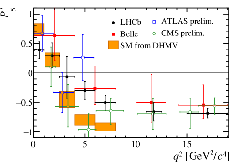
Figure 3: Observable $P_{5}^{\prime}$ measured by LHCb LHCb-PAPER-2015-051 and Belle Abdesselam:2016llu as a function of the dimuon invariant mass squared, $q^{2}$, in the $B\!\rightarrow{{K}^{*}}{\mu^{+}\mu^{-}}$ decay. Preliminary results from ATLAS ATLAS-CONF-2017-023 and CMS CMS-PAS-BPH-15-008 are also included. The shaded regions indicate theoretical predictions from Ref. Descotes-Genon:2014uoa .

3 Rare $B$-decays and the heavy quark expansion (S. Jäger)

3.1 Context

In the Standard Model (SM), the amplitude for a rare semileptonic decay $\bar{B}\rightarrow M\ell^{+}\ell^{-}$, with $M$ a hadronic system such as $\bar{K}$, $\bar{K}\pi,\dots$ can be written, to leading order in the electromagnetic coupling $\alpha_{\rm EM}$ but exact in QCD, as

$${\cal A}(B\rightarrow M\ell^{+}\ell^{-})=L^{\mu}a_{V\mu}+L^{5\mu}a_{A\mu},$$ (6)

where $L^{\mu}$ and $L^{5\mu}$ are the vector and axial lepton currents. One can trade $a_{V\mu}$, $a_{A\mu}$ for helicity amplitudes $H_{V\lambda}(q^{2})$ and $H_{A\lambda}(q^{2})$, where $\lambda$ is the helicity of the dilepton, which coincides with that of the hadronic state. For a kaon, $\lambda=0$ and there are two hadronic amplitudes. For a narrow $K^{*}$, $\lambda=\pm 1$ and there are six amplitudes. These amplitudes determine all rate and angular observables measured at $B$-factories and LHCb (where the lepton spins are not measured).

In the conventions of Jager:2012uw , $H_{A\lambda}\propto C_{10}V_{\lambda}(q^{2}),$ where $V_{\lambda}$ are form factors and $C_{10}$ is the axial semileptonic Wilson coefficient. (We omitted a normalisation free of hadronic uncertainties.) Note that $C_{10}$ and $V_{\lambda}$ are renormalisation-scale and -scheme-independent. $C_{10}$, in fact, receives no contributions from below the weak scale at all — this is what makes $B_{s}\rightarrow\mu^{+}\mu^{-}$ such a precision observable. The vector amplitudes can be written Jager:2012uw

$$H_{V\pm} \propto\left[C_{9}(\mu)V_{\pm}(q^{2})+\frac{2m_{b}m_{B}}{q^{2}}C_{7}^{\rm eff}(\mu)T_{\pm}(q^{2},\mu)-16\pi^{2}\frac{m_{B}^{2}}{q^{2}}h_{\pm}(q^{2},\mu)\right],$$ (7)

$$H_{V0} \propto\frac{\lambda^{1/2}}{2m_{B}\sqrt{q^{2}}}\left[C_{9}(\mu)V_{0}(q^{2})+\frac{2m_{b}}{m_{B}}C_{7}^{\rm eff}(\mu)T_{0}(q^{2},\mu)\right]-16\pi^{2}\frac{m_{B}^{2}}{q^{2}}h_{0}(q^{2},\mu).$$ (8)

Here $C_{9}(\mu)$ denotes the vector semileptonic Wilson coefficient, $T_{\lambda}$ tensor form factors, multiplied by the “effective” dipole Wilson coefficient $C_{7}^{\rm eff}$, and $h_{\lambda}\sim\langle M(\lambda)|T\left\{j^{\rm em,had}(y){\cal H}_{\rm had}^{\rm eff}(0)\right\}|\bar{B}\rangle$ denotes the contribution from the hadronic weak Hamiltonian (see Jager:2012uw for a precise definition). So far everything is exact from a QCD point of view. The theoretical difficulty resides in the evaluation of $h_{\lambda}$, which the heavy-quark expansion achieves, and of the form factors, for which the heavy-quark expansion provides relations.

One notes that $C_{9}(\mu)$ and $C_{7}^{\rm eff}(\mu)$ are strongly scale-dependent. E.g., at NNLL order, $C_{9}(10{\rm GeV})=3.75$, $C_{9}(5{\rm GeV})=4.18$, $C_{9}(2.5{\rm GeV})=4.49$. (One may compare this variation to a putative $\Delta C_{9}^{\rm BSM}\sim-1$.) The scale dependence must be precisely cancelled by the non-perturbative object $h_{\lambda}$. (This follows from RG-invariance of the Hamiltonian, which is exact.) Any quantitative theoretical description of $h_{\lambda}$ must correctly incorporate this.

3.2 The heavy-quark expansion

In the heavy-quark, large-recoil limit $E_{M},m_{B}\gg\Lambda$, where $\Lambda$ is the QCD scale parameter, $h_{\lambda}$ factorizes into perturbative hard-scattering kernels multiplying form factors and light-cone distribution amplitudes for the light meson $M=K,K^{*}$ Beneke:2001at ; Bosch:2001gv ; Beneke:2004dp , known as QCD factorization. It applies in the $q^{2}$-region below the narrow charm resonances, and perhaps above the charm threshold up to $q^{2}\sim 15{\rm GeV}^{2}$. QCDF can be formulated in soft-collinear effective field theory (SCET) language Becher:2005fg . “Factorization” is used in the Wilsonian sense of separating physics of the scales $\sqrt{\Lambda m_{b}}$, $m_{b}$, and above from the physics of the scale $\Lambda$, not to be confused with “naive factorization.” There are two distinct classes of effect. Vertex corrections may be compactly written as

$$C_{9} \rightarrow C_{9}(\mu)+Y(\mu,q^{2},m_{c})+\frac{\alpha_{s}}{4\pi}Y^{(1)}(\mu,q^{2},m_{c}),$$ (9)

$$C_{7}^{\rm eff} \rightarrow C_{7}^{\rm eff}(\mu)+\frac{\alpha_{s}}{4\pi}Z^{(1)}(\mu,q^{2},m_{c}),$$ (10)

where $Y,Y^{(1)}$,and $Z^{(1)}$ contain loop functions and Wilson coefficients. This form makes the helicity independence of these effects evident. The combination $C_{9}+Y$ is traditionally called $C_{9}^{\rm eff}(q^{2})$; the heavy-quark limit justifies its use, but also predicts model-independent higher-order corrections. (Note that $C_{9}$ starts at ${\cal O}(1/\alpha_{s})$ in the logarithmic counting, so $Y$ is formally a NLL correction.) The r.h.s. of (9),(10) are $\mu$-independent up to ${\cal O}(\alpha_{s}^{2})$ corrections. The other class of effects constitutes so-called hard spectator scattering and includes an annihilation contribution at ${\cal O}(\alpha_{s}^{0})$, though the latter comes with small CKM-factors and Wilson coefficients. Spectator scattering probes the structure of the $B$ and $K^{*}$-mesons through their light-cone distribution amplitudes and is helicity dependent (and vanishes for $\lambda=+$). Schematically,

$$h_{\lambda}^{\rm spec}\propto T_{\lambda}(\alpha_{s})*\phi_{B_{\pm}}*\phi_{K^{*}}.$$ (11)

This expression is separately scale-independent, resulting in formally $\mu$-independent observables. Corrections to the heavy-quark limit scale like $\Lambda/m_{B}$ and do not factorize, and must be estimated in other ways.

The expressions so far are sufficient to express all observables in terms of form factors Altmannshofer:2008dz , one can then use form factor results from light-cone sum rules to compute observables. Alternatively, one can make use of the fact that the heavy-quark large-recoil limit also implies relations between different form factors Charles:1998dr ; Beneke:2000wa ; Beneke:2003pa . They look extremely simple in the helicity basis,

$$T_{\lambda}(q^{2})=V_{\lambda}(q^{2})[1+f_{\lambda}(q^{2},\alpha_{s})]+\mbox{spectator scattering}+{\cal O}(\Lambda/m_{B})$$ (12)

for $\lambda=-,0$ and $T_{+}(q^{2})=V_{+}(q^{2})={\cal O}(\Lambda/m_{B})$. (The latter together with $h_{+}=0$ implies $H_{V+}=H_{A+}=0$.) Here $f_{\lambda}$ is a perturbative expression starting at ${\cal O}(\alpha_{s})$. The spectator-scattering contribution has a form similar to (11), and is again proportional to $\alpha_{s}$. All ${\cal O}(\alpha_{s}^{2})$ corrections are also known Beneke:2004rc ; Hill:2004if ; Becher:2004kk ; Beneke:2005gs . Note that the ratios $T_{\lambda}/V_{\lambda}$ are free of hadronic input in the heavy-quark limit, up to (calculable) spectator-scattering and (incalculable) power corrections.

There is an alternative expansion, applicable at $M_{B}^{2},q^{2}\gg\Lambda^{2}$, in particular above the $D\bar{D}$ threshold. The actual expansion is in $E_{M}/\sqrt{q^{2}}$ and expresses $h_{\lambda}$ in terms of matrix elements of local operators (OPE) of increasing dimension, again with perturbatively calculable coefficients Buchalla:1998mt ; Grinstein:2004vb ; Beylich:2011aq . This is not by itself a heavy-quark expansion, although the kinematics ensure that a HQE is valid and the $b$-quark field may be expanded accordingly Grinstein:2004vb , and the HQE can be used to estimate the matrix elements Beylich:2011aq . The leading matrix elements are again the form factors $T_{\lambda}$ and $V_{\lambda}$, with perturbative coefficient functions that coincide with $C_{7}^{\rm eff}$ and $C_{9}^{\rm eff}(q^{2})$ but different $\alpha_{s}$-corrections. The leading higher-dimensional corrections are of order $\Lambda^{2}/q^{2}$ and negligible, in particular spectator scattering is (strongly) power-suppressed. The OPE also gives a qualitative picture how open-charm resonances arise, by means of analytic continuation of OPE remainder terms from spacelike to physical (timelike) $q$, $\exp(-c\sqrt{-q^{2}}/\Lambda)\rightarrow\exp(-ic\sqrt{q^{2}}/\Lambda)$, giving oscillatory behaviour. Note that these “duality-violating” terms are nonanalytic in $\Lambda$, hence the large-recoil $\Lambda/m_{B}$ expansion will not capture them either. Formally such terms are of “infinite order” in $\Lambda/\sqrt{q^{2}}$ or $\Lambda/m_{B}$. They become less important away from the threshold and partly cancel out in binned observables (see Beylich:2011aq ; Lyon:2014hpa ). See also the discussion of charm resonances in $B\rightarrow K^{(*)}\mu^{+}\mu^{-}$ in Section 5.

3.3 Phenomenology

How large are the various effects and residual uncertainties? The shift to $C_{7}^{\rm eff}$ is an ${\cal O}(25\%)$ constructive correction. The ${\cal O}(\alpha_{s})$ correction to $C_{9}$ is an order $5\%$ destructive effect which partly cancels the ${\cal O}(\alpha_{s}^{0})$ term i.e. $Y(q^{2})$. The spectator-scattering corrections are smaller, though the normalisation is quite uncertain (by about a factor of two) due to the poor knowledge of the $B$-meson LCDA $\phi_{B_{+}}$. Overall the effects are significant. For instance, $\lim_{q^{2}\rightarrow 0}[q^{2}H_{V-}(q^{2})]$ gives the $B\rightarrow K^{*}\gamma$ amplitude, which receives a $+30\%$ correction, or a $+70\%$ correction at the rate level. Because $C_{7}^{\rm eff}$ is tightly constrained from the measured $B\rightarrow X_{s}\gamma$ rate, this allowed Beneke:2001at to conclude that, absent large power corrections, $T_{-}(0)=T_{1}(0)=0.27\pm 0.04$, updated to $T_{1}(0)=0.28\pm 0.02$ in Beneke:2004dp and well below LCSR predictions at the time. A recent LCSR evaluation Straub:2015ica gives $T_{1}(0)=0.308\pm 0.031$. The consistency supports smallness of power corrections.

It is impossible to give a comprehensive phenomenology of angular $B\rightarrow K^{*}\mu^{+}\mu^{-}$ observables in this space. Two observables that are very sensitive to $C_{9}$ are the forward-backward asymmetry, specifically its zero-crossing, and the angular term $S_{5}$ (or $P_{5}^{\prime}$). As long as Wilson coefficients are real, the FBAS zero is determined by ${\rm Re}\,H_{V-}(q_{0}^{2})=0$, up to second-order power corrections ${\cal O}(\Lambda^{2}/m_{B}^{2})$. From (7) it is clear that the zero depends on $(C_{7}^{\rm eff}/C_{9})\times(T_{-}/V_{-})$, essentially free from form-factor uncertainties in the heavy-quark limit. Given the fact that $C_{7}^{\rm eff}$ is essentially pinned to its SM value by $B\rightarrow X_{s}\gamma$, a $q^{2}_{0}$-measurement may hence be viewed as a determination of $C_{9}$. Ref. Beneke:2004dp obtained $q^{2}_{0}=4.36^{+0.33}_{-0.31}$ GeV² (neglecting power corrections), to be compared to the LHCb determination LHCb-PAPER-2015-051 $q^{2}_{0}\in[3.40,4.87]$ GeV², in good agreement. By comparison, the LCSR form factors of Straub:2015ica imply a lower crossing point, around $3.5$ GeV², giving a slight preference for $C_{9}<C_{9}^{\rm SM}$. This can be traced to a ratio of $T_{-}/V_{-}$ that is ${\cal O}(10\%)$ below the heavy-quark-limit prediction, which is still consistent with a power correction. The eventual relative accuracy on $C_{9}$ is limited by that on ratio $T_{-}(q_{0}^{2})/V_{-}(q_{0}^{2})$.

The observable $P_{5}^{\prime}$ Matias:2012xw , which shows the most pronounced anomaly, depends on all six helicity amplitudes. It hence depends on ratios $T_{-}/V_{-}$, $T_{0}/V_{0}$, $V_{+}/V_{-}$, $T_{+}/V_{-}$, and $V_{0}/V_{-}$. The last of these does not satisfy a heavy-quark relation, but $P_{5}^{\prime}$ has been constructed in such a way that dependence on it cancels in the heavy-quark limit if $\alpha_{s}$-corrections are neglected. It has been suggested to employ $V\propto V_{+}+V_{-}$ instead of $V_{-}$ Descotes-Genon:2014uoa , which reduces the explicit sensitivity to $V_{+}$ in $P_{5}^{\prime}$. From a pure heavy-quark perspective, the physics of $V_{+}$ (which involves soft physics flipping the helicity of the strange quark emitted from $b$-quark decay, or changing the helicity of the $B$-remnant absorbed into the $K^{*}$) and $V_{-}$ (which does not require such a spin-flip) seem very different, such that the conservative choice is to associate separate uncertainties to both (hence a larger one to $V$). The impact on the significance of the $P_{5}^{\prime}$ anomaly is noticeable because of this Jager:2014rwa ; Descotes-Genon:2014uoa and because Descotes-Genon:2014uoa adopt central values for power corrections to match LCSR form factor central values while Jager:2014rwa use zero central values (the HQ limit). Further recent investigations on the role of power corrections in semileptonic $B$-decays can be found in Ciuchini:2016weo ; Capdevila:2017ert ; Chobanova:2017ghn .

3.4 Discussion

The heavy-quark expansion goes a long way to putting rare $B$ decays on a systematic theoretical footing, and rightly has found its place at the heart of many phenomenological works and fits to BSM effects. In particular it removes most of the ambiguities of older “$C_{7,9,10}$ + resonances” approaches. Its primary limitations are incalculable power corrections. There is no evidence that these are abnormally large. Rather, the fact that they matter in the interpretation of anomalies points to the impressive precision that experiment has already reached (and the apparent smallness of possible BSM effects). At the moment, there is no first-principles method to compute power corrections. Light-cone sum rule calculations can provide information. As they carry their own uncontrolled systematics, it would be particularly desirable to have sum rule results directly for the power-suppressed terms, where possible. Combining these with the leading-power expressions would remove most of the systematics of either framework. One example is the sum rule Khodjamirian:2010vf for $h_{+}(q^{2})$, which vanishes in the heavy-quark limit. One finds an extra (ie double) power suppression of this term at $q^{2}\approx 0$, which implies an excellent sensitivity to $C_{7}^{\prime}$ Jager:2012uw ; Jager:2014rwa . Data-driven approaches may be able to constrain some of the power corrections, especially if data in very small bin-sizes becomes available for $B\rightarrow K^{*}\mu^{+}\mu^{-}$. This path has been followed to some extent in Ciuchini:2015qxb .

4 Form-factors (Z.Liu & R.Zwicky)

Form-factors (FFs) describe the short-distance part of the transition amplitudes. For hadronic transitions of the type $B\rightarrow M$ at the quark level $b\rightarrow q$ they consist of matrix elements of the form $\langle M(p)|\bar{s}\Gamma b|\bar{B}(p_{B})\rangle$. For $M$ being a light meson the FFs can be computed from light-cone sum rules (LCSR) and lattice QCD at low and high momentum transfer $q^{2}=(p_{B}-p)^{2}$ respectively. The ones most relevant to the current discussion of flavour anomalies are the $B\rightarrow V$ ($V=K^{*},\phi,\dots$) FFs which follow from the vector and tensor current (cf. $O_{9,10}$ and $O_{7}$ in (1))

$$\langle K^{*}(p,\eta)|\bar{s}\gamma^{\mu}(1\mp\gamma_{5})b|\bar{B}(p_{B})\rangle \;=\; \;\;P_{1}^{\mu}\,{\cal V}_{1}(q^{2}) \;\pm\; P_{2}^{\mu}\,{\cal V}_{2}(q^{2}) \;\pm\; P_{3}^{\mu}\,{\cal V}_{3}(q^{2})\pm P_{P}^{\mu}{\cal V}_{P}(q^{2})\;,$$

$$\langle K^{*}(p,\eta)|\bar{s}iq_{\nu}\sigma^{\mu\nu}(1\pm\gamma_{5})b|\bar{B}(p_{B})\rangle \;=\; \;\;P_{1}^{\mu}T_{1}(q^{2}) \;\pm\; P_{2}^{\mu}T_{2}(q^{2}) \;\pm\; P_{3}^{\mu}T_{3}(q^{2})\;,$$ (13)

where we have chosen $V=K^{*}$ as a matter of concreteness. Above $P_{1,2,3,P}$ are Lorentz structures involving the $K^{*}$-meson polarisation vector $\eta$ and momenta and the structures ${\cal V}_{1,2,3,P}$ are more commonly known as the $V$, $A_{2,3,0}$ FFs Straub:2015ica . Below we summarise the status of these computations in LCSR & lattice, discuss the issue of the finite width of the $K^{*}$-meson and the use of the equation of motion (EOM) on eliminating uncertainties. The FFs are fitted by a $z$-expansion, with flat priors on the coefficients, to the lattice Horgan:2013hoa ; Horgan:2015vla and LCSR Straub:2015ica data. The latter are pseudo-data generated from the analytic LCSR computation with a Markov chain process Straub:2015ica . The thereby obtained error correlation matrix reduces the $10\%$-uncertainty of individual FFs by a considerable amount, which is relevant for $B\rightarrow K^{*}\ell\ell$-decay angular distributions.

4.1 Status of LCSR and lattice computations

LCSR FFs are computed from a light-cone OPE, valid at $q^{2}\leq O(m_{b}\Lambda)\simeq 14\mathrm{\,Ge\kern-1.00006ptV}^{2}$ in an $\alpha_{s}$- and twist-expansion resulting in convolutions of a hard kernel and light-cone distribution amplitudes (LCDA). The LCDA are subjected to equations of motion (EOMs) and are relatively well-known to the necessary order in the conformal partial wave expansion (e.g. Gegenbauer moments). For $B\rightarrow V$ ($B_{(q,s)}\rightarrow(K^{*},\phi,\rho,\omega)$) FFs, defined in (13) the FFs are known up to twist-3 at $O(\alpha_{s}^{3})$ and twist-4 $O(\alpha_{s}^{0})$ Ball:2004rg ; Straub:2015ica . State-of-the-art computations of $B\rightarrow K$ LCSR FFs, for which the DAs are better known because of the absence of finite width effects, can be found in Ball:2004ye ; Khodjamirian:2010vf .

Lattice QCD calculations are based on the path integral formalism in Euclidean space. The QCD theory is discretized on a finite space time lattice. Correlation functions, from which FFs can be extracted, are then obtained by solving the integrals numerically using Monte Carlo methods. Since both the noise to signal ratio of correlation functions and discretization effects increase as the momenta of hadrons increase, lattice QCD results cover the high $q^{2}$ region at $\sim 15\mbox{ GeV}^{2}\leq q^{2}\leq q^{2}_{\mbox{max}}$ for $B\rightarrow V$ ($B_{(q,s)}\rightarrow(K^{*},\phi)$) FFs. Unquenched calculations are available for 2+1-flavor dynamical fermions Horgan:2013hoa ; Horgan:2015vla ; Flynn:2016vej in the narrow width approximation of the vector mesons. $B\rightarrow K$ FFs can be found in Bouchard:2013pna ; Bailey:2015dka for 2+1-flavor dynamical configurations.

4.2 Finite width effects

The vector meson decays via the strong force, e.g. $K^{*}\rightarrow K\pi$ and do therefore have a sizeable width and it is legitimate to ask how each formalism deals with this issue.

For LCSR the answer is surprisingly pragmatic in that the formalism automatically adapts to the experimental handling of the vector meson resonance. In LCSR the vector meson is described by LCDAs, which we may schematically write as

$$\langle K^{*}(p,\eta)|\bar{s}(x)\gamma_{\mu}q(0)|0\rangle=m_{K^{*}}f_{K^{*}}p_{\mu}\int_{0}^{1}due^{up\cdot x}\phi_{\parallel}(u)+\text{higher twist}\;,$$ (14)

where $p=m_{K^{*}}\eta$, valid upon neglecting the higher twist corrections $O(x^{2},m_{K}^{*})$, has been assumed. The variable $u$ is the momentum fraction of the $s$-quark in the infinite momentum frame and the DA $\phi_{\parallel}(u)$ parametrises the strength of the higher Gegenbauer moments (conformal spin). Since the latter contribute only about $10$-$15\%$ at the numerical level the main part is effectively described by the $K^{*}$-meson decay constant $f_{K^{*}}$. Hence at the pragmatic level the issue of finite width effects is the same as to how well-defined the decay constant $f_{K^{*}}$ is.

Whereas the latter can be computed from QCD sum rules or lattice modulo finite width effects it is advantageous to directly extract it from experiment (e.g. $\tau\rightarrow K^{*}\nu$ and cf. appendix C in Ref. Straub:2015ica for a review). Consistency is ensured if in both cases, leptonic $\tau\rightarrow(K\pi)_{l=1}\nu$ and hadronic decay $B\rightarrow(K\pi)_{l=1}\ell\ell$, the experimentalist employs the same fit ansatz for the resonances and the continuous background in the p-wave ($l=1$) $K\pi$-channel. The transversal decay constant $f_{K^{*}}^{\perp}$, is not directly accessible in experiment. It is preferably taken from the ratio $f_{K^{*}}/f_{K^{*}}^{\perp}$ which can be computed from QCD sum rules or lattice QCD for which one would expect finite width effects to drop out in ratios. This is a reasonable and testable hypothesis. In conclusion a consistent treatment of the $K^{*}$ in experiments allows us to bypass a first principle definition of the $K^{*}$-meson as a pole on the second sheet and the induced error can be seen as negligible compared to the remaining uncertainty.

A fully controlled lattice QCD computation of FFs involving a vector meson needs to include scattering states. This requires much more sophisticated and expensive calculations. In existing lattice calculations of the FFs, the threshold effects are assumed to be small in the narrow width approximation. Since the $\phi$ is relatively narrow, one might expect this approximation to be better than in the case of $K^{*}$. For $B\rightarrow D^{*}$ form-factors, heavy meson chiral perturbation theory predicts 1-2% threshold effects Randall:1993qg ; Hashimoto:2001nb which is unfortunately not indicative since it is enhanced and also outside any linear regime as compared to the broad light vector meson $\Gamma_{D^{*}}/\Gamma_{K^{*}}\sim O(10^{-2})$. An encouraging aspect is though that the continuum- and chiral-extrapolated lattice FFs obtained in Horgan:2013hoa ; Horgan:2015vla agree with LCSR results, upon $z$-expansion extrapolation, despite the two methods having very different systematic uncertainties. Finite width effects can only be fully assessed from a systematic computation to which the Maiani-Testa no-go theorem Maiani:1990ca is an obstruction. The latter states that there is no simple relation between Euclidean ( lattice QCD) correlators and the transition matrix elements in Minkowski space when multiple hadrons are involved in the initial or final states. The first formalism to overcome this problem is the Lellouch-Lüscher method Lellouch:2000pv which relates matrix elements of currents in finite volume to those in the infinite volume. Further developments of this formalism can be found in, for examples, Refs. Hansen:2012tf ; Briceno:2014uqa ; Dudek:2014qha ; Prelovsek:2013ela ; Wilson:2014cna ; Agadjanov:2016fbd . Their implementations for $B\rightarrow K\pi$-type matrix elements may be hoped for in the foreseeable future.

4.3 The use of the equations of motion (projection on $B$-meson ground state)

Both in LCSR and lattice computations the $B$-meson is described by an interpolating current and it is therefore a legitimate question what the precision of the projection on the $B$-meson ground state is. Below we argue that the EOMs improve the situation.

The vector and tensor operators entering (13) are related by EOMs

$$\langle K^{*}|i\partial^{\nu}(\bar{s}i\sigma_{\mu\nu}b)|B\rangle \;=\; -(m_{s}\pm m_{b})\langle K^{*}|\bar{s}\gamma_{\mu}b|B\rangle \;+\; i\partial_{\mu}\langle K^{*}|(\bar{s}b)|B\rangle\;, \;-\; 2\langle K^{*}|\bar{s}i\!\stackrel{{\scriptstyle\leftarrow}}{{D}}_{\mu}b|B\rangle$$

$$\quad\sim T_{1}(q^{2}) \;=\; \quad\sim{\cal V}_{1}(q^{2}) \;+\; \quad\sim 0 \;+\; \quad\sim{\cal D}_{1}(q^{2})$$ (15)

where the derivative term defines a new FF ${\cal D}_{1}(q^{2})$ in analogy to $T_{1}(q^{2})$. The EOM (4.3) are exact and have to be obeyed and therefore can be used as a non-trivial check for any computation. This has been done in Straub:2015ica at the tree-level up to twist-4 and for the $Z$-factors describing the renormalisation of the composite operators entering the EOM (4.3). Furthermore at the level of the effective Hamiltonian this term is redundant, since the EOMs have been used in reducing the basis of operators. Eq.(4.3) therefore defines a relation between 3 FFs of which one is redundant which does not appear helpful at first. The use comes from the hierarchy ${\cal D}_{1}\ll T_{1},{\cal V}_{1}$ which therefore constrains the vector in terms of the tensor FF Hambrock:2013zya ; Straub:2015ica . At the level of the actual computation this allows us to control the correlation of the continuum threshold parameters which are a major source of uncertainty for the individual FFs. The argument is that if those parameters were to differ by a sizeable amount for the vector and tensor form factors then the exactness of (4.3) would impose a huge shift for the corresponding parameters of the derivative FF corresponding to an absurd violation of semi-global quark hadron duality. Since ${\cal D}_{1}$ seems to be a FF with normal convergence in $\alpha_{s}$ and the twist-expansion this possibility seems absurd and therefore supports the validity of the argument. It should be mentioned that the crucial hierarchy ${\cal D}_{1}\ll T_{1},{\cal V}_{1}$ can be traced back to the large energy limit Charles:1998dr . For more details and a plot illustrating the validity of this argument over the $q^{2}$-range we refer the reader to references Hambrock:2013zya ; Straub:2015ica and Fig.1 in Straub:2015ica .

On the lattice the projection on the ground state would be perfect if one could go to infinite Euclidean time and if there was no noise. In practice simulations are done at a finite $t$-interval with some noise and this sets some limitations on the projection. On the positive side these aspects are not the main sources of uncertainties in current LQCD calculations (smearing and other methods are being used to improve the projection) and are improvable with more computer power. It is conceivable that the EOMs can be used for the lattice in correlating the projection of FFs entering the same EOM.

5 The relevance of charm contributions (R.Zwicky)

5.1 The LCSR framework

The long distance contributions can be computed with LCSR as an alternative to the heavy quark framework discussed in section 3.2. The basic long distance topologies are well-known and include the chromomagnetic operator $O_{8}$ (1), the weak annihilation (WA), quark-spectator loop scattering (QQLS) and the charm contributions. The latter three originate from the four quark operators $O_{1..6}$ in (1). The charm contributions are presumably the most relevant since they are not CKM suppressed with sizeable Wilson coefficients and are the subject of a longer discussion in Sec. 5.2. For $B\rightarrow K^{(*)}\ell\ell$ and other final state hadrons the $O_{8}$ and WA contribution have been computed in Dimou:2012un and Lyon:2013gba respectively. Both come with strong phases and the first one is found to be small whereas the second one is rather sizeable albeit CKM suppressed. The quark spectator scattering diagrams have been computed in a hyprid approach of heavy quark expansion with infrared divergences removed by an LCSR computation Lyon:2013gba .

Whereas we agree that the heavy quark expansion provides a systematic framework in the $1/m_{b}$-limit for regions outside the resonance regions it has to be seen that in practice these conditions are not always met for $b\rightarrow s\ell\ell$ observables. Since LCSR are not dependent on the $1/m_{b}$-limit they do provide an alternative to estimate these effects. In Sec. 5.2 we argue that the $1/m_{b}$ vertex corrections might well be sizeable, contributing to potential tension in $b\rightarrow s\ell\ell$-observables. Resonant effects can be systematically parameterised and fitted for but their inclusion into predictions requires further thought and work when a sizeable continuum contributions is present.

5.2 The charm contribution

In FCNC processes of the type $B\rightarrow K^{(*)}\ell\ell$, the subprocess $B\rightarrow K^{(*)}(\bar{c}c\rightarrow\gamma^{*}\rightarrow\ell\ell)$ is numerically relevant since it proceeds at tree-level. Hence the Wilson coefficients of operators of the type $O^{(c)}_{1,2}$ (1) in the effective Hamiltonian are sizeable. The other relevant aspect is that the four momentum invariant, $q^{2}\in[4m_{\ell}^{2},(m_{B}-m_{K^{(*)}})^{2}]$, of the lepton-pair takes on values in the region of charmonium resonances. Hence the process is sensitive to resonances, with photon quantum numbers $J^{PC}=1^{--}$, and one can therefore not entirely rely on a partonic picture. It is customary to divide the $q^{2}$-spectrum into three regions (cf.Fig. 4). A region sufficiently well-below the first charmonium resonance at $q^{2}=m_{{{J\mskip-3.0mu/\mskip-2.0mu\psi\mskip 2.0mu}}}^{2}\simeq 9.6\mathrm{\,Ge\kern-1.00006ptV}^{2}$, the region of the two narrow charmonium resonances ${{J\mskip-3.0mu/\mskip-2.0mu\psi\mskip 2.0mu}}$ and $\psi(2S)$ and the region of broad charmonium states above the $\bar{D}D$-threshold $q^{2}\simeq 14\mathrm{\,Ge\kern-1.00006ptV}^{2}$. The crucial question is when and how partonic methods are applicable in the hadronic charmonium region. We discuss them below in the order of tractability in the partonic picture.

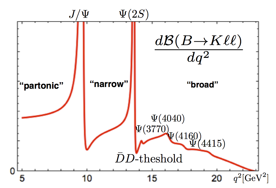
Figure 4: Illustration of the spectrum in $q^{2}$, the lepton pair invariant momentum, for the $B\rightarrow K\ell\ell$ branching fraction. The three regions referred to in the text are the “below resonance region" (partonic, low-$q^{2}$), “narrow resonance region" and the “broad resonance region" (high-$q^{2}$).

In the “below-charmonium region" partonic methods (i.e. $\alpha_{s}$-expansion ) are expected to be applicable. Since this is the region where the particles are fast in the $B$-rest frame, the physics can be described within a light-cone formalism. The order $O(\alpha_{s}^{0})$ contribution is equivalent to naive factorisation (NF) which means that the amplitude factorises as follows

$${\cal A}[B\rightarrow K^{(*)})\ell\ell]\Big{|}^{\text{NF}}_{O^{(c)}_{1,2}}\sim h(q^{2})F^{B\rightarrow K^{(*)}}(q^{2})\;,$$ (16)

where $F^{B\rightarrow K^{(*)}}(q^{2})$ stands for the relevant form factor (FF) combination and $h(q^{2})$ is the vacuum polarisation due to the charm-part of the electromagnetic current. At this formal level the light-cone aspect is only present in that the preferred methodology for evaluating the FFs are light-cone methods (cf. Sec. 4.1). Corrections of order $O(\alpha_{s})$ are expected to be sizeable since the leading order contribution is of the colour-suppressed Wilson coefficient combination. Simple factorisation formulae only hold in the $1/m_{b}$-limit which include hard spectator and vertex corrections Bosch:2001gv ; Beneke:2001at with the latter borrowed from inclusive computations Asatrian:2001de . The $O(\alpha_{s}/m_{b})$ corrections can be done within an extended LCSR approach with either a $B$- or $K^{(*)}$-meson LCDA. Only partial results exist in that the vertex and hard spectator corrections have not been evaluated in either of these methods. The third contribution, emission of the gluon into the LCDA, have been done for $K^{(*)}$- and $B$-meson Ball:2006eu ; Muheim:2008vu (computations for $q^{2}=0$ only) and Khodjamirian:2010vf respectively. The reason that the vertex and hard spectator corrections have not been performed in either approach is that they are technically demanding. If one insists on verifying the dispersion relation involved this demands an evaluation of a two-loop graph with five scales and an integration over one LCDA-parameter. The size of these contributions is therefore unknown beyond the heavy quark limit and might well be sizeable enough to explain the current picture of deviations even within a partonic approach. A completion of this program is therefore desirable.

The broad charmonium region (see Fig. 4 on the right) is characterised by a considerable interference of the short-distance and charmonium long-distance part. The charmonium resonances $\psi(3770)$, $\psi(4040)$, $\psi(4160)$ and $\psi(4415)$ are broad because of they can decay via the strong force into $\bar{D}D$-states. The resonances are necessarily accompanied by a continuum of $\bar{D}D$-states as is the case in $e^{+}e^{-}\rightarrow hadrons$. Lyon:2014hpa . A sketch of a realistic parametrisation is given by

$${\cal A}[B\rightarrow K^{(*)})\ell\ell]\Big{|}_{O^{(c)}_{1,2}}\simeq\sum_{\psi={{J\mskip-3.0mu/\mskip-2.0mu\psi\mskip 2.0mu}},\psi(2S),\psi(3770),..}\frac{r_{\psi}}{q^{2}-m_{\psi}^{2}+im_{\psi}\Gamma_{\psi}}+f_{\bar{c}c}(q^{2})\;,$$ (17)

where the residues $r_{\psi}$ and the non-resonant $\bar{c}c$-continuum function $f_{\bar{c}c}$ are the unknowns which usually have to be determined experimentally. For $e^{+}e^{-}\rightarrow hadrons$, which correspond effectively to NF (16), $r_{\psi}^{\text{NF}}\sim\Gamma(\psi\rightarrow\ell\ell)F^{B\rightarrow K^{(*)}}(m_{\psi}^{2})>0$ and $\text{Im}[f^{\text{NF}}_{\bar{c}c}(q^{2})]>0$ for which successful parametrisations are easily found and the real part follows from a dispersion relation Ablikim:2007gd ; Lyon:2014hpa . Going beyond factorisation involves determining the factors $\eta_{\psi}$ and the continuum function $f_{\bar{c}c}(q^{2})$

$$\eta_{\psi}\equiv|\eta_{\psi}|e^{i\delta_{\psi}}=\frac{r_{\psi}}{r_{\psi}^{\text{NF}}}\;,\qquad f_{\bar{c}c}(q^{2})\;.$$ (18)

The strong-phase $\delta_{\psi}$ is defined relative to the FF contribution. The determination of $f_{\bar{c}c}(q^{2})$ is a difficult task since the $q^{2}$-dependence is similar to the one of the short distance contributions. On the other hand the shape of the resonances is very distinct (e.g Fig. 4) and can therefore be fitted unambiguously. This has been done in Lyon:2014hpa using the LHCb-data LHCb-PAPER-2013-039 . A surprisingly good fit is obtained by $\eta_{\tilde{\psi}}\simeq-2.55$ and $\delta_{\tilde{\psi}}\simeq 0$ with $\tilde{\psi}\in\{\psi(3770),\psi(4040),\psi(4160),\psi(4415)\}$. One concludes that NF is badly broken and that the charm might impact on the low $q^{2}$-spectrum Lyon:2014hpa . For example, even in the narrow width approximation the non-local part of the resonances (17) only decays as $1/q^{2}$ away from its centre.

These results bring the focus to the “narrow charmonium region". Whereas the absolute values $|\eta_{{{J\mskip-3.0mu/\mskip-2.0mu\psi\mskip 2.0mu}}}|\simeq 1.4$ and $|\eta_{\psi(2S)}|\simeq 1.8$ are known from the decay rates $\Gamma(B\rightarrow K^{(*)}\psi)$ the phases $\delta_{{{J\mskip-3.0mu/\mskip-2.0mu\psi\mskip 2.0mu}},\psi(2S)}$ are unknown. The need to extract these from experiment has been emphasised and suggested in Lyon:2014hpa and recently been performed by LHCb collaboration Aaij:2016cbx . Unfortunately, so far, the solutions show a four-fold ambiguity $(\delta_{{{J\mskip-3.0mu/\mskip-2.0mu\psi\mskip 2.0mu}}}|\delta_{\psi(2S)})\simeq(0,\pi|0,\pi)$. Whereas this is an important result one would hope that this ambiguity can be resolved with more data in the future.

After this excursion let us discuss the practicalities for the low-$q^{2}$ (“below resonance region") and the high-$q^{2}$ (“broad resonance region") regions where phenomenologists and experimentalists compare predictions to measurements in the hope of seeing physics beyond the Standard Model. It would be desirable to obtain a coherent picture of the partonic and hadronic descriptions in both of these regions in order to validate the approaches. Both cases need more work. At low-$q^{2}$, as discussed above, the partonic contributions are not very complete. For example, the potentially sizeable vertex corrections of the charm loop are unknown beyond the $1/m_{b}$-limit. There is no universal or well-understood pattern for estimating the size of the $1/m_{b}$-corrections. For example the FF $1/m_{b}$-corrections are around $10\%$, for the $B$-meson decay constant $f_{B}$ they are $30\%$ whereas for the $O_{8}$-matrix elements (chromomagnetic operator) they are $50\%$ and more Dimou:2012un . As for the hadronic data, further work is needed in order to determine the strong phases $\delta_{{{J\mskip-3.0mu/\mskip-2.0mu\psi\mskip 2.0mu}},\psi(2S)}$ as well as the continuum function $f_{\bar{c}c}(q^{2})$. Before moving on it should be mentioned that the hadronic fits should and will be extended from $B\rightarrow K\ell\ell$ to $B\rightarrow K^{*}\ell\ell$ by the LHCb-collaboration. In the high-$q^{2}$ region a partonic picture has been advocated, known as the high-$q^{2}$ OPE, where one resorts to an expansion in $1/m_{b}$ and $1/\sqrt{q^{2}}$ supplemented by charm-contributions Grinstein:2004vb ; Beylich:2011aq . The initial idea was to include charm contributions in an $\alpha_{s}$-expansion, relying on cancellations when averaged over large enough bins. As an estimate of these type of quark-hadron duality violations for the broad resonances, naive factorisation (i.e. $e^{+}e^{-}\rightarrow hadrons$) was taken as guidance Beylich:2011aq , which suggests an effect of the order of $2\%$. One is then faced with the a posteriori fact that the actual data LHCb-PAPER-2013-039 show effects in the region of $10\%$ Lyon:2014hpa . Hence supplementing the high-$q^{2}$ OPE with a hadronic representation (17) seems attractive. The bottleneck is though the determination of the the continuum function $f_{\bar{c}c}(q^{2})$ (17). A promising direction could be the experimental investigation of the $B\rightarrow\bar{D}DK^{(*)}$ modes.

5.2.1 Discussion and summary

Clarifying the role of the charm will remain an outstanding task before angular anomalies of the $B\rightarrow K^{*}\ell\ell$-type and branching fraction deviations, not related to violation of lepton flavour universality (LFU), can be considered to be physics beyond the Standard Model. Progress can be made by computing charm contributions consistently in one approach, complemented by more refined experimental data allowing us to extract the relevant information. Hopefully this will pursued by experimentalists and theorists.

Finally, a few brief comments on LFU-violation, the possibility of new physics in charm and right-handed currents. Clarifying the role of LFU-violating observables, e.g. $R_{K}$ (5), is of importance for global fits. QED corrections, which can give rise to $O(\alpha_{\text{QED}}\ln^{2}(m_{\mu}/m_{e}))$-deviations from $R_{K}=1$, can be diagnosed by higher moments Gratrex:2015hna . The dominant real radiation effect has been estimated in Bordone:2016gaq and crucially the effect deviates by $O(1\%)$ as compared to the PHOTOS-implementation Golonka:2005pn used by the LHCb-analysis. Migration of narrow charmonium events into lower $q^{2}$-region by misidentification of hadronic final states Gratrex:2015hna has been checked by the LHCb-collaboration. The fact that charm contributions can mimic shifts in $C_{9}$, or any other amplitude with photon quantum numbers, has been emphasised in Lyon:2014hpa motivated by the results on the broad charmonium resonances in $B\rightarrow K\ell\ell$. In this work it was suggested to diagnose this effect with $q^{2}$-dependent fits in various $b\rightarrow s\ell\ell$-channels, and the question as to whether the anomalies could partially be due to new physics in charm (e.g. $\bar{b}c\bar{c}s$-operators) was raised. The former idea was applied to $B\rightarrow K^{*}\ell\ell$ at low $q^{2}$ for the first time in  Altmannshofer:2015sma , and the possibility of charm in new physics was recently investigated systematically including RG-evolution and constraints (e.g. $B_{s}$-mixing) in Jager:2017gal . A closely related area where charm contributions are of importance is the search for right-handed currents. The V-A structure of the weak interactions and the small ratio $m_{s}/m_{b}$ suppress amplitudes with right-handed quantum numbers that can, for instance, be measured in time-dependent CP-asymmetries Atwood:1997zr . Charm contributions, of higher-twist, are a non-perturbative background to these measurements, whose understanding is important. LHCb’s first time measurement of the $B_{s}\rightarrow\phi\gamma$ time-dependent CP-asymmetry ${\cal A}_{\Delta}\simeq-0.98(50)(20)$ Aaij:2016ofv comes with a large uncertainty but also with a large deviation from the SM prediction ${\cal A}_{\Delta}\simeq 0.047(28)$ Muheim:2008vu , which allows for speculations in various directions.

6 Global fits (L. Hofer)

As reported in Sec. 2, experimental results on $B\rightarrow K^{*}\mu^{+}\mu^{-}$, $B_{s}\rightarrow\phi\mu^{+}\mu^{-}$ and $R_{K}=Br(B\rightarrow K\mu^{+}\mu^{-})/Br(B\rightarrow Ke^{+}e^{-})$ show deviations from the SM at the $2-3\sigma$ level. Although none of these tensions is yet significant on its own, the situation is quite intriguing as the affected decays are all mediated by the same quark-level transition $b\rightarrow s\ell^{+}\ell^{-}$ and thus probe the same high-scale physics. A correlated analysis of these channels can shed light on the question whether a universal new-physics contribution to $b\rightarrow s\ell^{+}\ell^{-}$ can simultaneously alleviate the various tensions and lead to a significantly improved global description of the data.

At the energy scale of the $B_{(s)}$ decays, any potential high-scale new physics mediating $b\rightarrow s\ell^{+}\ell^{-}$ transitions can be encoded into the effective couplings $C_{7,9,10}^{(\prime)}$ multiplying the operators

$$\mathcal{O}_{9}^{(\prime)}=\frac{\alpha}{4\pi}[\bar{s}\gamma^{\mu}P_{L(R)}b][\bar{\mu}\gamma_{\mu}\mu],\hskip 28.45274pt\mathcal{O}_{10}^{(\prime)}=\frac{\alpha}{4\pi}[\bar{s}\gamma^{\mu}P_{L(R)}b][\bar{\mu}\gamma_{\mu}\gamma_{5}\mu],$$

$$\mathcal{O}_{7}^{(\prime)}=\frac{\alpha}{4\pi}m_{b}[\bar{s}\sigma_{\mu\nu}P_{R(L)}b]F^{\mu\nu},$$ (19)

where $P_{L,R}=(1\mp\gamma_{5})/2$ and $m_{b}$ denotes the $b$ quark mass. Whereas the above-mentioned semi-leptonic decays are sensitive to the full set $C_{7,9,10}^{(\prime)}$ of effective couplings, the decay $B_{s}\rightarrow\ell^{+}\ell^{-}$ only probes $C_{10}^{(\prime)}$ and $B\rightarrow X_{s}\gamma$, $B\rightarrow K^{*}\gamma$ set constraints on $C_{7}^{(\prime)}$. Note that additional scalar or pseudoscalar couplings $C_{S,S^{\prime},P,P^{\prime}}$ cannot address the tensions in exclusive semi-leptonic $B$ decays since their contributions are suppressed by small lepton masses.

Coefficient	Best fit	1$\sigma$	PullSM
$C_{7}^{\rm NP}$	$-0.02$	$[-0.04,-0.00]$	1.2
$C_{9}^{\rm NP}$	$-1.09$	$[-1.29,-0.87]$	4.5
$C_{10}^{\rm NP}$	$0.56$	$[0.32,0.81]$	2.5
$C_{7}^{\prime\rm NP}$	$0.02$	$[-0.01,0.04]$	0.6
$C_{9}^{\prime\rm NP}$	$0.46$	$[0.18,0.74]$	1.7
$C_{10}^{\prime\rm NP}$	$-0.25$	$[-0.44,-0.06]$	1.3
$C_{9}^{\rm NP}=C_{10}^{\rm NP}$	$-0.22$	$[-0.40,-0.02]$	1.1
$C_{9}^{\rm NP}=-C_{10}^{\rm NP}$	$-0.68$	$[-0.85,-0.50]$	4.2
$C_{9}^{\rm NP}=-C_{9}^{\prime\rm NP}$	$-1.06$	$[-1.25,-0.85]$	4.8

Fit	$C_{9\ \rm Bestfit}^{\rm NP}$	1$\sigma$	PullSM
All $b\rightarrow s\mu\mu$	$-1.09$	$[-1.29,-0.87]$	4.5
$b\rightarrow s\mu\mu$ without $q^{2}\in[6,8]$	$-0.99$	$[-1.23,-0.75]$	3.8
$b\rightarrow s\mu\mu$ large recoil	$-1.30$	$[-1.57,-1.02]$	4.0
$b\rightarrow s\mu\mu$ low recoil	$-0.93$	$[-1.23,-0.61]$	2.8
Only $B\rightarrow K\mu\mu$	$-0.85$	$[-1.67,-0.20]$	1.4
Only $B\rightarrow K^{*}\mu\mu$	$-1.05$	$[-1.27,-0.80]$	3.7
Only $B_{s}\rightarrow\phi\mu\mu$	$-1.98$	$[-2.84,-1.29]$	3.5

Table 1: Left: best-fit point, 1$\sigma$ region and SM-pull for 1-parameter fits allowing new physics only in one of the couplings $C_{7,9,10}^{(\prime)}$. Right: fits of a new-physics contribution to the effective coupling $C_{9}$ using different subsets of the experimental data as input. Results are taken from Ref. Descotes-Genon:2015uva

Various groups have performed fits of the couplings $C_{7,9,10}^{(\prime)}$ to the data Descotes-Genon:2013wba ; Altmannshofer:2013foa ; Altmannshofer:2014rta ; Descotes-Genon:2015uva ; Hurth:2016fbr . The obtained results are in mutual agreement with each other and confirm the observation, pointed out for the first time in Ref. Descotes-Genon:2013wba on the basis of the 2013 data, that a large negative new-physics contribution $C_{9}$ yields a fairly good description of the data. This is illustrated in Tab. 1, where selected results from Ref. Descotes-Genon:2015uva for one-parameter fits of the couplings $C_{7,9,10}^{(\prime)}$ are displayed. Apart from the best-fit point together with the $1\sigma$ region, the tables feature the SM-pull of the respective new-physics scenarios. This number quantifies by how many sigmas the best fit point is preferred over the SM point $\{C_{i}^{\rm NP}\}=0$ and thus measures the capacity of the respective scenario to accommodate the data. The table on the left demonstrates that a large negative new-physics contribution $C_{9}$ is indeed mandatory to significantly improve the quality of the fit compared to the SM. It is particularly encouraging that the individual channels tend to prefer similar values for $C_{9}$, as shown in the table on the right.

The results of the fit are quite robust with respect to the hadronic input and the employed methodology. This can be seen from the good agreement between the results of the analyses AS Altmannshofer:2014rta and DHMV Descotes-Genon:2015uva which use approaches that are complementary in many respects:

• AS choose the observables $S_{i}$ as input for the fit to the angular distributions of $B\rightarrow K^{*}\ell^{+}\ell^{-}$ and $B_{s}\rightarrow\phi\ell^{+}\ell^{-}$ and restrict their fits in the region of large $K^{*}$-recoil to squared invariant dilepton masses $q^{2}\in[0,6]$ GeV². DHMV, on the other hand, choose the observables $P_{i}^{(\prime)}$, which feature a reduced sensitivity to the non-perturbative form factors, and include all bins up to $q^{2}=8$ GeV².

• AS use LCSR form factors from Ref. Straub:2015ica , while DHMV mainly resort to the LCSR form factors from Ref. Khodjamirian:2010vf .

• In the analysis of AS, correlations among the form factors are implemented on the basis of the LCSR calculation Straub:2015ica , whereas in the analysis of DHMV they are assessed from large-recoil symmetries supplemented by a sophisticated estimate of symmetry-breaking corrections of order $\mathcal{O}(\Lambda/m_{b})$. The pros and cons of these two methods complement each other: The first approach provides a more complete access of correlations at the price of a dependence on and the limitation to one particular LCSR calculation Straub:2015ica and its intrinsic model-assumptions. The second approach determines the correlations in a model-independent way from first principles but needs to rely on an estimate of subleading non-perturbative $\Lambda/m_{b}$ corrections.

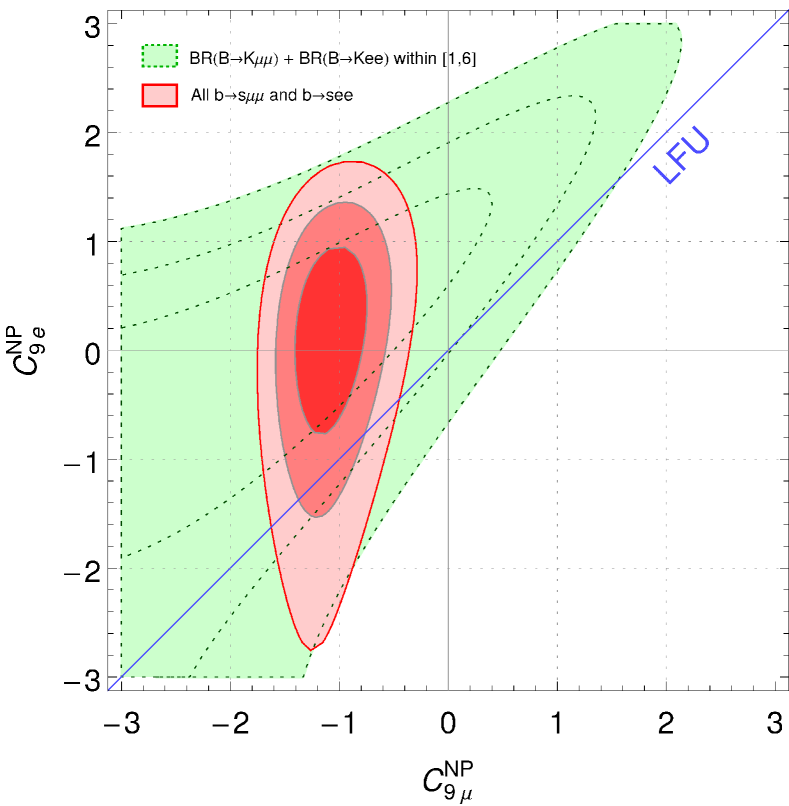
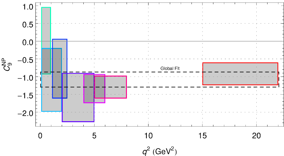
Figure 5: Left: Fit allowing for LFUV by means of independent coefficients $C_{9\;\mu}^{\rm NP}$ and $C_{9\;e}^{\rm NP}$. Right: Bin-by-bin fit of the one-parameter scenario with a single coefficient $C_{9}^{\rm NP}$. Reproduced from Ref. Descotes-Genon:2015uva .

The measurement of $R_{K}\neq 1$ hints at a possible violation of lepton-flavour universality (LFUV) and suggests a situation where the muon- and the electron-components of the operators $C_{9,10}^{(\prime)}$ receive independent new-physics contributions $C_{i\;\mu}^{\rm NP}$ and $C_{i\;e}^{\rm NP}$, respectively. In Fig. 5 on the left we display the result for the two-parameter fit to the coefficients $C_{9\;\mu}^{\rm NP}$ and $C_{9\;e}^{\rm NP}$. The plot is taken from Ref. Descotes-Genon:2015uva , similar results are obtained in Refs. Altmannshofer:2014rta ; Hurth:2016fbr . The fit prefers an electron-phobic scenario with new physics coupling to $\mu^{+}\mu^{-}$ but not to $e^{+}e^{-}$. Under this hypothesis, that should be tested by measuring $R_{K^{*},\phi}$ as well as lepton-flavour sensitive angular observables Capdevila:2016ivx  , the SM-pull increases by $\sim 0.5\sigma$ compared to the value in Tab. 1 for the lepton-flavour universal scenario, except for the scenario with $C_{9}^{\rm NP}=-C_{9}^{\prime\rm NP}$ where the value remains unchanged due to the absence of any contribution to $R_{K}$.

The fact that it is primarily the variation of the coefficient $C_{9}$ which is responsible for solving the anomalies unfortunately spoils an unambiguous interpretation of the fit results in terms of new physics. The reason is that precisely this effective coupling can be mimicked by non-perturbative charm loops, as discussed in Sec. 5. However, whereas these non-local effects are expected to introduce a non-trivial dependence on the squared invariant mass $q^{2}$ of the lepton pair, a high-scale new-physics solution would necessarily generate a $q^{2}$ independent $C_{9}^{\rm NP}$. A promising strategy to resolve the nature of a potential non-standard contribution to the effective coupling $C_{9}$ thus consists in the investigation of its $q^{2}$ dependence. To this end, two different methods have been pursued so far: In Ref. Altmannshofer:2015sma , the authors performed a bin-by-bin fit of $C_{9}$ to check whether results in different bins were consistent with each other under the hypothesis of a $q^{2}$-independent $C_{9}$. Their conclusion, which was later confirmed also in Ref. Descotes-Genon:2015uva with the plot shown in Fig. 5 on the right, was that there is no indication for a $q^{2}$-dependence, though the situation is not conclusive due to the large uncertainties in the single bins.

An alternative strategy to address this question has been followed recently in Refs. Ciuchini:2015qxb ; Capdevila:2017ert where a direct fit of the $q^{2}$-dependent charm contribution $C_{9}^{c\bar{c}\;i}(q^{2})$ to the data on $B\rightarrow K^{*}\mu^{+}\mu^{-}$ (at low $q^{2}$) has been performed under the hypothesis of the absence of new physics. The results are in agreement with the findings from Fig. 5: in Ref. Capdevila:2017ert it was shown that the inclusion of additional terms parametrising a non-trivial $q^{2}$-dependence does not improve the quality of the fit. On the other hand, current precision of the experimental data does not allow to exclude non-zero values for these terms.

In certain scenarios, a $q^{2}$-dependent contribution to $C_{9}$ can also have its origin at high energy scales: new physics mediating $b\rightarrow sc\bar{c}$ transitions would induce a $q^{2}$-dependent contribution to $b\rightarrow s\ell^{+}\ell^{-}$ at the one-loop level in the effective theory. This possibility was proposed for the first time in Ref. Lyon:2014hpa , while a phenomenological analysis taking into account constraints from $B_{s}-\bar{B}_{s}$ mixing and $B\rightarrow X_{s}\gamma$ was performed recently in Ref. Jager:2017gal . Note that a charm-loop contribution to $b\rightarrow s\ell^{+}\ell^{-}$, whether from high-scale new physics or from low-energy QCD dynamics, always conserves lepton flavour and thus could not account for deviations in $R_{K}$ or other LFUV observables.

7 BSM interpretation (L. Hofer)

As we have seen in the previous section, the observed anomalies in $b\rightarrow s\ell^{+}\ell^{-}$ decays show a coherent picture and allow for a solution at the level of the effective Hamiltonian by NP contributions to the operators $\mathcal{O}^{(\prime)}_{9,10}$. At tree level, contributions to these operators can be mediated by exchange of a heavy neutral vector-boson $Z^{\prime}$ (e.g. Descotes-Genon:2013wba ; Buras:2013qja ; Gauld:2013qja ; Buras:2013dea ; Altmannshofer:2014cfa ; Celis:2015ara ; Falkowski:2015zwa ; Crivellin:2015mga ; Crivellin:2015lwa ; Crivellin:2015era ; Becirevic:2016zri ; Boucenna:2016qad ; Crivellin:2016ejn ), or by scalar or vector lepto-quarks (e.g. Hiller:2014yaa ; Gripaios:2014tna ; Becirevic:2015asa ; Varzielas:2015iva ; Fajfer:2015ycq ; Becirevic:2016yqi ). At one loop, they can be generated by box diagrams involving new particles (e.g. Gripaios:2015gra ; Bauer:2015knc ; Arnan:2016cpy ) or by $Z^{\prime}$ penguins (e.g. Belanger:2015nma ). The step beyond the model-independent analysis allows to attempt a common explanation of the $b\rightarrow s\ell^{+}\ell^{-}$ anomalies with other tensions in flavour data, like $R_{D^{(*)}}$ or the long-standing anomaly in the anomalous magnetic moment of the muon. It further permits to study the viability of the various model classes in the light of constraints from other flavour observables and from direct searches. In the following, we will briefly summarize typical $Z^{\prime}$ and lepto-quark scenarios, and discuss bounds from $B_{s}-\overline{B}_{s}$ mixing and direct searches.

7.1 $Z^{\prime}$ models

The interaction of a generic $Z^{\prime}$ boson with the SM fermions is described by the Lagrangian

$$\mathcal{L}_{Z^{\prime}}\,=\,\sum\limits_{ff^{\prime}}\Gamma^{L}_{ff^{\prime}}\bar{f}\gamma^{\mu}P_{L}f^{\prime}Z^{\prime}_{\mu}\,+\,\Gamma^{R}_{ff^{\prime}}\bar{f}\gamma^{\mu}P_{R}f^{\prime}Z^{\prime}_{\mu}\,+\,{\text{h}.c.},$$ (20)

where the sum is over fermions $f,f^{\prime}$ with equal electric charges. The exact form of the couplings $\Gamma^{L,R}_{ij}$ depends on the $U(1)^{\prime}$ charges assigned to the SM fermions and on a potential embedding of the $Z^{\prime}$ in a more fundamental theory. Note, however, that SU$(2)_{L}$ invariance implies the model-independent relations $\Gamma^{L}_{uu^{\prime}}=V_{ud}\Gamma^{L}_{dd^{\prime}}V^{\dagger}_{u^{\prime}d^{\prime}}$ and $\Gamma^{L}_{\ell\ell^{\prime}}=\Gamma^{L}_{\nu_{\ell}\nu_{\ell^{\prime}}}$ (with $V$ denoting the CKM matrix).

The Wilson coefficients $C_{9,10}^{(\prime)}$ are generated by tree-level $Z^{\prime}$ exchange involving products of couplings $\Gamma^{L,R}_{bq}\,\Gamma^{L,R}_{\ell\ell}$. Since only three out of these four products are independent, the relation $C_{9}\cdot C_{10}^{\prime}\,=\,C_{9}^{\prime}\cdot C_{10}$ is fulfilled in models with a single $Z^{\prime}$ boson. In order to generate a non-vanishing coupling $C_{9\,\mu}$, mandatory for a solution of the $b\rightarrow s\ell^{+}\ell^{-}$ anomalies, the couplings $\Gamma_{bs}^{L}$ and $\Gamma_{\mu\mu}^{L}+\Gamma_{\mu\mu}^{R}$ need to have non-vanishing values.

The most popular class of $Z^{\prime}$ models is based on gauging $L_{\tau}-L_{\mu}$ lepton number Altmannshofer:2014cfa ; Crivellin:2015mga ; Crivellin:2015lwa ; Altmannshofer:2015mqa ; Altmannshofer:2016oaq . This pattern of $U(1)^{\prime}$ charges avoids anomalies and is well-suited to generate the measured PMNS matrix. The vanishing coupling of the $Z^{\prime}$ to electrons allows to explain LFUV in $R_{K}$ and helps to avoid LEP bounds on the $Z^{\prime}$ mass $M_{Z^{\prime}}$. The symmetry can be extended to the quark sector with a flavour non-universal assignment of $U(1)^{\prime}$ charges that induces the off-diagonal couplings $\Gamma^{L,R}_{bs}$ ( e.g. Crivellin:2015lwa ; Celis:2015ara ). An alternative mechanism to generate the couplings $\Gamma^{L,R}_{bs}$ consists in the introduction of additional vector-like quarks that are charged under the $U(1)^{\prime}$ symmetry and that generate an effective $bsZ^{\prime}$ coupling via their mixing with the SM fermions Altmannshofer:2014cfa ; Crivellin:2015mga ; Altmannshofer:2015mqa ; Bobeth:2016llm .

Several $Z^{\prime}$ scenarios have been proposed that are capable of solving not only the $b\rightarrow s\ell^{+}\ell^{-}$ anomalies but at the same time also other tensions in the data. Embedding the $Z^{\prime}$ in a SU$(2)^{\prime}$ gauge model allows to address the anomalies in $R_{D^{(*)}}$ with a tree-level contribution to $b\rightarrow c\ell^{-}\bar{\nu}$ mediated by the $W^{\prime}$-boson (e.g. Greljo:2015mma ; Boucenna:2016qad ). It is also possible to solve the anomaly in $(g-2)_{\mu}$ in a $Z^{\prime}$ scenario, provided the $Z^{\prime}$ coupling to muons is generated at the loop-level so that both the NP contributions to $b\rightarrow s\ell^{+}\ell^{-}$ and $(g-2)_{\mu}$ are loop-suppressed Belanger:2015nma .

7.2 Lepto-quark models

Lepto-quarks are new particles $\Delta_{k}$ beyond the SM that couple leptons to quarks via vertices $\ell_{i}q_{j}\Delta_{k}$. Different lepto-quark models can be classified according to the spin of the lepto-quarks and their quantum numbers with respect to the SM gauge groups. Since the $\ell_{i}q_{j}\Delta_{k}$ couplings violate lepton-flavour, lepto-quark models are excellent candidates to explain LFUV observables like $R_{K}$ and $R_{D^{(*)}}$. Indeed, various representations of lepto-quarks have been studied with respect to their capability of accommodating the measured values of $R_{K}$ and $R_{D^{(*)}}$ by tree-level lepto-quark contributions Hiller:2014yaa ; Gripaios:2014tna ; Becirevic:2015asa ; Varzielas:2015iva ; Fajfer:2015ycq ; Becirevic:2016yqi . In Ref. Bauer:2015knc it was further proposed that an SU$(2)_{L}$ singlet scalar lepto-quark could explain $R_{D^{(*)}}$ by a tree-level and $R_{K}$ by a loop contribution. This possibility was later shown in Ref. Becirevic:2016oho to be challenged by other flavour data.

7.3 Constraints from $B_{s}-\overline{B}_{s}$ mixing and direct searches

A NP model generating $b\rightarrow s\ell^{+}\ell^{-}$ necessarily also contributes to $B_{s}-\bar{B}_{s}$ mixing. In lepto-quark models, $b\rightarrow s\ell^{+}\ell^{-}$ is typically mediated at tree level, while $B_{s}-\bar{B}_{s}$ mixing contributions are loop-suppressed and thus do not pose relevant contraints. In $Z^{\prime}$ models, on the other hand, both processes are usually generated by tree-level exchange of the $Z^{\prime}$ boson. The constraint on $|\Gamma^{L,R}_{bs}|/M_{Z^{\prime}}$ from $B_{s}-\bar{B}_{s}$ mixing then imposes a lower limit of typically $|\Gamma^{L,R}_{\mu\mu}|/M_{Z^{\prime}}\gtrsim 0.3/(1\,\textrm{TeV})$ that needs to be reached for a solution of the $b\rightarrow s\mu^{+}\mu^{-}$ anomalies. In models with box contributions to both $b\rightarrow s\ell^{+}\ell^{-}$ and $B_{s}-\overline{B}_{s}$ mixing, the analogous constraint is more severe due to the loop suppression: $|\Gamma_{\mu}|/\sqrt{M_{\Phi}}\gtrsim 3/\sqrt{1\,\textrm{TeV}}$ where $M_{\Phi}$ denotes the mass scale of the new particles in the box and $\Gamma_{\mu}$ their coupling strength to the muon. It was shown in Ref. Arnan:2016cpy that this bound can be relaxed in a scenario with Majorana fermions in the box where the additional crossed boxes lead to a negative interference in $B_{s}-\overline{B}_{s}$ mixing.

Bounds from direct searches can be avoided to a large extent if the new physics couples only to the second and third fermion generation, in line with LFUV in $R_{K}$ and $R_{D^{(*)}}$. Collider signals are then limited to more complex final state, like e.g. $pp\rightarrow 4\mu$ probing the muon-coupling of a possible $Z^{\prime}$ boson, or to suppressed production channels, like e.g. $b\bar{s}\rightarrow\mu^{+}\mu^{-}$. However, it was found Faroughy:2016osc very recently that the data from Atlas/CMS already now heavily constrains $Z^{\prime}$ and lepto-quark scenarios even in the $b\bar{b}\rightarrow\tau^{+}\tau^{-}$ channel: a solution of $R_{D^{(*)}}$ by SU$(2)^{\prime}$ gauge bosons $W^{\prime}/Z^{\prime}$ is restricted to masses $M_{Z^{\prime}}\lesssim 500\,\textrm{GeV}$, and a solution via vector lepto-quarks is about to be excluded. The interplay with high-$p_{T}$ searches will thus definitely play a crucial role in the quest for an explanation of the flavour anomalies.

8 Summary

The discovery of the leptonic decay ${{B}^{0}_{s}}\!\rightarrow{\mu^{+}}{\mu^{-}}$ by the CMS and LHCb collaborations was a major breakthrough of precision flavour physics with data from Run 1 of the Large Hadron Collider. Since then, several anomalies have emerged in semileptonic decays. These indicate a potential violation of lepton universality in the decays $B\!\rightarrow K^{(*)}{\mu^{+}\mu^{-}}$ and $B\!\rightarrow K^{(*)}{e^{+}}{e^{-}}$ with a statistical significance of $2.6\sigma$. In the angular analysis of $B\!\rightarrow K^{*}{\mu^{+}\mu^{-}}$ decays, tensions with the SM are seen in the longitudinal polarisation of the $K^{*}$ and the angular observable $P_{5}^{\prime}$. The largest discrepancy with more than $3\sigma$ is seen in the differential branching fraction of the decay ${{B}^{0}_{s}}\!\rightarrow\phi{\mu^{+}\mu^{-}}$.

The dynamics of $B\!\rightarrow K^{*}{\mu^{+}\mu^{-}}$ decays can be described by a set of helicity amplitudes, which, in the effective Hamiltonian formalism, split into Wilson coefficients and matrix elements of local operators. Deviations in the Wilson coefficient $C_{9}$, which is sensitive to new physics as well as long-distance QCD, can explain the experimental data. The most sensitive observables to $C_{9}$ are the $q^{2}$ dependence of the forward-backward asymmetry and the angular observable $P_{5}^{\prime}$. These observables have been constructed such that they exhibit a reduced sensitivity to hadronic form factors, though a remnant dependence at order $\Lambda/m_{{b}}$ cannot be avoided and its impact cannot be predicted in the heavy quark framework. A combination of light-cone sum rule calculations with more precise measurements may be able to address this issue.

In light-cone sum rule computation finite width effects can effectively be bypassed if the vector mesons are treated consistently in all experiments, which includes those from where input is taken for form factor calculations as well as those where the form factor computations are used. Whereas current lattice QCD studies do not include finite width effects, recent developments indicate that this may change in the foreseeable future. The use of equation of motion reduces the uncertainty of the projection on the $B$-meson state for ratios of form factors in light-cone sum rules. It is conceivable that the use of equation of motion might help to further improve lattice QCD computation as well.

The main focus of recent discussions have been the so-called charm contributions, which describe the sub-process $B\rightarrow K^{(*)}(\bar{c}c\rightarrow\gamma^{*}\rightarrow\ell\ell)$. The data are typically studied in different regions of $q^{2}$: the ‘partonic’ well below the ${J\mskip-3.0mu/\mskip-2.0mu\psi\mskip 2.0mu}$ resonance, the ‘narrow’ between the ${J\mskip-3.0mu/\mskip-2.0mu\psi\mskip 2.0mu}$ and $\psi(2S)$ resonances, and the ‘broad’ in the high-$q^{2}$ region that is dominated by broad charmonium resonances. Ideally, a coherent description of the low and high $q^{2}$ regions should be obtained. Overcoming these challenges requires close collaboration of experimentalists and theorists to pursue new approaches such as a detailed study of the decays $B\!\rightarrow{\kern 1.99997pt\overline{\kern-1.99997ptD}{}}DK^{(*)}$.

Global fits aim to exploit a maximum of information of the range of observables in the framework of an effective theory. This allows the splitting of the Wilson coefficients in a SM part and a component to encapsulate effects beyond the SM. Most fits favour a non-SM value of the coefficient $C_{9}$ of about $-1$ with the pull of the SM scenario exceeding $4\sigma$ in several cases. As contributions from high scales beyond the SM create $q^{2}$-independent effects, it is instructive to perform fits in several regions of $q^{2}$ and test for $q^{2}$-dependent effects that would indicate low-scale SM effects. At the current level of precision these tests are consistent with a $q^{2}$-independent shift of $C_{9}$.

Possible explanations involving particles beyond the SM exist in the form of lepto-quarks or $Z^{\prime}$ bosons, typically mediating the ${b}\!\rightarrow{s}\ell^{+}\ell^{-}$ transitions through tree-level exchange. In addition, these SM extensions have the potential to simultaneously accommodate other anomalies like $R_{D^{(*)}}$ or the anomalous magnetic moment of the muon. Direct searches pose tight constraints on some of these models and are expected to either probe or severely challenge them in the near future.

The number of flavour anomalies that appear to fit a common picture is intriguing. The analysis of data taken during the ongoing Run 2 of the LHC will yield powerful new insight both into the observables of interest and into new strategies to control uncertainties. The interpretation of these results requires close collaboration with theory, where advances are required in several areas for which promising strategies exist.

References

- (1) H. Albrecht et al. (ARGUS collaboration), Phys. Lett. B192, 245 (1987), [,51(1987)]
- (2) C. Bobeth, M. Gorbahn, T. Hermann, M. Misiak, E. Stamou, M. Steinhauser, Phys. Rev. Lett. 112, 101801 (2014), 1311.0903
- (3) V. Khachatryan et al. (CMS and LHCb collaborations), Nature 522, 68 (2015), 1411.4413
- (4) M. Aaboud et al. (ATLAS collaboration), Eur. Phys. J. C76, 513 (2016), 1604.04263
- (5) R. Aaij et al. (LHCb collaboration), JHEP 06, 133 (2014), 1403.8044
- (6) R. Aaij et al. (LHCb collaboration), JHEP 09, 179 (2015), 1506.08777
- (7) V. Khachatryan et al. (CMS collaboration), Phys. Lett. B753, 424 (2016), 1507.08126
- (8) R. Aaij et al. (LHCb collaboration), Phys. Rev. Lett. 111, 112003 (2013), 1307.7595
- (9) W. Altmannshofer, D.M. Straub, Eur. Phys. J. C75, 382 (2015), 1411.3161
- (10) A. Bharucha, D.M. Straub, R. Zwicky, JHEP 08, 098 (2016), 1503.05534
- (11) R.R. Horgan, Z. Liu, S. Meinel, M. Wingate, Phys. Rev. Lett. 112, 212003 (2014), 1310.3887
- (12) R. Aaij et al. (LHCb collaboration), Phys. Rev. Lett. 113, 151601 (2014), 1406.6482
- (13) P. Golonka, Z. Was, Eur.Phys.J. C45, 97 (2006), hep-ph/0506026
- (14) S. Agostinelli et al. (Geant4 collaboration), Nucl. Instrum. Meth. A506, 250 (2003)
- (15) J.P. Lees et al. (BaBar collaboration), Phys. Rev. D93, 052015 (2016), 1508.07960
- (16) J.T. Wei et al. (Belle collaboration), Phys. Rev. Lett. 103, 171801 (2009), 0904.0770
- (17) T. Aaltonen et al. (CDF collaboration), Phys. Rev. Lett. 108, 081807 (2012), 1108.0695
- (18) R. Aaij et al. (LHCb collaboration), JHEP 02, 104 (2016), 1512.04442
- (19) A. Abdesselam et al. (Belle collaboration) (2016), BELLE-CONF-1603, 1604.04042
- (20) Angular analysis of decays in collisions at TeV with the ATLAS detector, ATLAS collaboration, ATLAS-CONF-2017-023
- (21) Measurement of the and angular parameters of the decay in proton-proton collisions at TeV, CMS collaboration, CMS-PAS-BPH-15-008
- (22) S. Descotes-Genon, L. Hofer, J. Matias, J. Virto, JHEP 12, 125 (2014), 1407.8526
- (23) S. Jäger, J. Martin Camalich, JHEP 05, 043 (2013), 1212.2263
- (24) R. Aaij et al. (LHCb collaboration) (2016), 1612.06764
- (25) M. Beneke, T. Feldmann, D. Seidel, Nucl. Phys. B612, 25 (2001), hep-ph/0106067
- (26) S.W. Bosch, G. Buchalla, Nucl. Phys. B621, 459 (2002), hep-ph/0106081
- (27) M. Beneke, T. Feldmann, D. Seidel, Eur. Phys. J. C41, 173 (2005), hep-ph/0412400
- (28) T. Becher, R.J. Hill, M. Neubert, Phys. Rev. D72, 094017 (2005), hep-ph/0503263
- (29) W. Altmannshofer, P. Ball, A. Bharucha, A.J. Buras, D.M. Straub, M. Wick, JHEP 01, 019 (2009), 0811.1214
- (30) J. Charles, A. Le Yaouanc, L. Oliver, O. Pene, J.C. Raynal, Phys. Rev. D60, 014001 (1999), hep-ph/9812358
- (31) M. Beneke, T. Feldmann, Nucl. Phys. B592, 3 (2001), hep-ph/0008255
- (32) M. Beneke, T. Feldmann, Nucl. Phys. B685, 249 (2004), hep-ph/0311335
- (33) M. Beneke, Y. Kiyo, D.s. Yang, Nucl. Phys. B692, 232 (2004), hep-ph/0402241
- (34) R.J. Hill, T. Becher, S.J. Lee, M. Neubert, JHEP 07, 081 (2004), hep-ph/0404217
- (35) T. Becher, R.J. Hill, JHEP 10, 055 (2004), hep-ph/0408344
- (36) M. Beneke, D. Yang, Nucl. Phys. B736, 34 (2006), hep-ph/0508250
- (37) G. Buchalla, G. Isidori, Nucl. Phys. B525, 333 (1998), hep-ph/9801456
- (38) B. Grinstein, D. Pirjol, Phys. Rev. D70, 114005 (2004), hep-ph/0404250
- (39) M. Beylich, G. Buchalla, T. Feldmann, Eur. Phys. J. C71, 1635 (2011), 1101.5118
- (40) J. Lyon, R. Zwicky (2014), 1406.0566
- (41) J. Matias, F. Mescia, M. Ramon, J. Virto, JHEP 04, 104 (2012), 1202.4266
- (42) S. Jäger, J. Martin Camalich, Phys. Rev. D93, 014028 (2016), 1412.3183
- (43) M. Ciuchini, M. Fedele, E. Franco, S. Mishima, A. Paul, L. Silvestrini, M. Valli, in the Standard Model: Elaborations and Interpretations, in Proceedings, 38th International Conference on High Energy Physics (ICHEP 2016): Chicago, IL, USA, August 3-10, 2016 (2016), 1611.04338, https://inspirehep.net/record/1497744/files/arXiv:1611.04338.pdf
- (44) B. Capdevila, S. Descotes-Genon, L. Hofer, J. Matias (2017), 1701.08672
- (45) V.G. Chobanova, T. Hurth, F. Mahmoudi, D. Martinez Santos, S. Neshatpour (2017), 1702.02234
- (46) A. Khodjamirian, T. Mannel, A.A. Pivovarov, Y.M. Wang, JHEP 09, 089 (2010), 1006.4945
- (47) M. Ciuchini, M. Fedele, E. Franco, S. Mishima, A. Paul, L. Silvestrini, M. Valli, JHEP 06, 116 (2016), 1512.07157
- (48) R.R. Horgan, Z. Liu, S. Meinel, M. Wingate, Phys. Rev. D89, 094501 (2014), 1310.3722
- (49) R.R. Horgan, Z. Liu, S. Meinel, M. Wingate, PoS LATTICE2014, 372 (2015), 1501.00367
- (50) P. Ball, R. Zwicky, Phys. Rev. D71, 014029 (2005), hep-ph/0412079
- (51) A. Khodjamirian, T. Mannel, N. Offen, Phys. Rev. D75, 054013 (2007), hep-ph/0611193
- (52) P. Ball, R. Zwicky, Phys. Rev. D71, 014015 (2005), hep-ph/0406232
- (53) J. Flynn, T. Izubuchi, A. Juttner, T. Kawanai, C. Lehner, E. Lizarazo, A. Soni, J.T. Tsang, O. Witzel, Form factors for semi-leptonic decays, in 34th International Symposium on Lattice Field Theory (Lattice 2016) (2016), 1612.05112, https://inspirehep.net/record/1504065/files/arXiv:1612.05112.pdf
- (54) C. Bouchard, G.P. Lepage, C. Monahan, H. Na, J. Shigemitsu (HPQCD collaboration), Phys. Rev. D88, 054509 (2013), [Erratum: Phys. Rev.D88,no.7,079901(2013)], 1306.2384
- (55) J.A. Bailey et al., Phys. Rev. D93, 025026 (2016), 1509.06235
- (56) L. Randall, M.B. Wise, Phys. Lett. B303, 135 (1993), hep-ph/9212315
- (57) S. Hashimoto, A.S. Kronfeld, P.B. Mackenzie, S.M. Ryan, J.N. Simone, Phys. Rev. D66, 014503 (2002), hep-ph/0110253
- (58) L. Maiani, M. Testa, Phys. Lett. B245, 585 (1990)
- (59) L. Lellouch, M. Luscher, Commun. Math. Phys. 219, 31 (2001), hep-lat/0003023
- (60) M.T. Hansen, S.R. Sharpe, Phys. Rev. D86, 016007 (2012), 1204.0826
- (61) R.A. BriceÃo, M.T. Hansen, A. Walker-Loud, Phys. Rev. D91, 034501 (2015), 1406.5965
- (62) J.J. Dudek, R.G. Edwards, C.E. Thomas, D.J. Wilson (Hadron Spectrum collaboration), Phys. Rev. Lett. 113, 182001 (2014), 1406.4158
- (63) S. Prelovsek, L. Leskovec, C.B. Lang, D. Mohler, Phys. Rev. D88, 054508 (2013), 1307.0736
- (64) D.J. Wilson, J.J. Dudek, R.G. Edwards, C.E. Thomas, Phys. Rev. D91, 054008 (2015), 1411.2004
- (65) A. Agadjanov, V. Bernard, U.G. MeiÃner, A. Rusetsky, Nucl. Phys. B910, 387 (2016), 1605.03386
- (66) C. Hambrock, G. Hiller, S. Schacht, R. Zwicky, Phys. Rev. D89, 074014 (2014), 1308.4379
- (67) M. Dimou, J. Lyon, R. Zwicky, Phys. Rev. D87, 074008 (2013), 1212.2242
- (68) J. Lyon, R. Zwicky, Phys. Rev. D88, 094004 (2013), 1305.4797
- (69) H.H. Asatrian, H.M. Asatrian, C. Greub, M. Walker, Phys. Lett. B507, 162 (2001), hep-ph/0103087
- (70) P. Ball, G.W. Jones, R. Zwicky, Phys. Rev. D75, 054004 (2007), hep-ph/0612081
- (71) F. Muheim, Y. Xie, R. Zwicky, Phys. Lett. B664, 174 (2008), 0802.0876
- (72) M. Ablikim et al. (BES), eConf C070805, 02 (2007), [Phys. Lett.B660,315(2008)], 0705.4500
- (73) M. Beneke, G. Buchalla, M. Neubert, C.T. Sachrajda, Eur. Phys. J. C61, 439 (2009), 0902.4446
- (74) G. Hiller, R. Zwicky, JHEP 03, 042 (2014), 1312.1923
- (75) J. Gratrex, M. Hopfer, R. Zwicky, Phys. Rev. D93, 054008 (2016), 1506.03970
- (76) M. Bordone, G. Isidori, A. Pattori, Eur. Phys. J. C76, 440 (2016), 1605.07633
- (77) W. Altmannshofer, D.M. Straub, Implications of measurements, in Proceedings, 50th Rencontres de Moriond Electroweak Interactions and Unified Theories: La Thuile, Italy, March 14-21, 2015 (2015), pp. 333–338, 1503.06199, http://inspirehep.net/record/1353682/files/arXiv:1503.06199.pdf
- (78) S. JÃger, K. Leslie, M. Kirk, A. Lenz (2017), 1701.09183
- (79) D. Atwood, M. Gronau, A. Soni, Phys. Rev. Lett. 79, 185 (1997), hep-ph/9704272
- (80) R. Aaij et al. (LHCb), Phys. Rev. Lett. 118, 021801 (2017), [Addendum: Phys. Rev. Lett.118,no.10,109901(2017)], 1609.02032
- (81) S. Descotes-Genon, L. Hofer, J. Matias, J. Virto, JHEP 06, 092 (2016), 1510.04239
- (82) S. Descotes-Genon, J. Matias, J. Virto, Phys. Rev. D88, 074002 (2013), 1307.5683
- (83) W. Altmannshofer, D.M. Straub, Eur. Phys. J. C73, 2646 (2013), 1308.1501
- (84) T. Hurth, F. Mahmoudi, S. Neshatpour, Nucl. Phys. B909, 737 (2016), 1603.00865
- (85) B. Capdevila, S. Descotes-Genon, J. Matias, J. Virto, JHEP 10, 075 (2016), 1605.03156
- (86) S. Wehle et al. (Belle), Phys. Rev. Lett. 118, 111801 (2017), 1612.05014
- (87) A.J. Buras, J. Girrbach, JHEP 12, 009 (2013), 1309.2466
- (88) R. Gauld, F. Goertz, U. Haisch, JHEP 01, 069 (2014), 1310.1082
- (89) A.J. Buras, F. De Fazio, J. Girrbach, JHEP 02, 112 (2014), 1311.6729
- (90) W. Altmannshofer, S. Gori, M. Pospelov, I. Yavin, Phys. Rev. D89, 095033 (2014), 1403.1269
- (91) A. Celis, J. Fuentes-Martin, M. Jung, H. Serodio, Phys. Rev. D92, 015007 (2015), 1505.03079
- (92) A. Falkowski, M. Nardecchia, R. Ziegler, JHEP 11, 173 (2015), 1509.01249
- (93) A. Crivellin, G. D’Ambrosio, J. Heeck, Phys. Rev. Lett. 114, 151801 (2015), 1501.00993
- (94) A. Crivellin, G. D’Ambrosio, J. Heeck, Phys. Rev. D91, 075006 (2015), 1503.03477
- (95) A. Crivellin, L. Hofer, J. Matias, U. Nierste, S. Pokorski, J. Rosiek, Phys. Rev. D92, 054013 (2015), 1504.07928
- (96) D. BeÄireviÄ, O. Sumensari, R. Zukanovich Funchal, Eur. Phys. J. C76, 134 (2016), 1602.00881
- (97) S.M. Boucenna, A. Celis, J. Fuentes-Martin, A. Vicente, J. Virto, JHEP 12, 059 (2016), 1608.01349
- (98) A. Crivellin, J. Fuentes-Martin, A. Greljo, G. Isidori (2016), 1611.02703
- (99) G. Hiller, M. Schmaltz, Phys. Rev. D90, 054014 (2014), 1408.1627
- (100) B. Gripaios, M. Nardecchia, S.A. Renner, JHEP 05, 006 (2015), 1412.1791
- (101) D. Becirevic, S. Fajfer, N. Kosnik, Phys. Rev. D92, 014016 (2015), 1503.09024
- (102) I. de Medeiros Varzielas, G. Hiller, JHEP 06, 072 (2015), 1503.01084
- (103) S. Fajfer, N. Kosnik, Phys. Lett. B755, 270 (2016), 1511.06024
- (104) D. Becirevic, S. Fajfer, N. Kosnik, O. Sumensari, Phys. Rev. D94, 115021 (2016), 1608.08501
- (105) B. Gripaios, M. Nardecchia, S.A. Renner, JHEP 06, 083 (2016), 1509.05020
- (106) M. Bauer, M. Neubert, Phys. Rev. Lett. 116, 141802 (2016), 1511.01900
- (107) P. Arnan, L. Hofer, F. Mescia, A. Crivellin (2016), 1608.07832
- (108) G. Belanger, C. Delaunay, S. Westhoff, Phys. Rev. D92, 055021 (2015), 1507.06660
- (109) W. Altmannshofer, I. Yavin, Phys. Rev. D92, 075022 (2015), 1508.07009
- (110) W. Altmannshofer, M. Carena, A. Crivellin, Phys. Rev. D94, 095026 (2016), 1604.08221
- (111) C. Bobeth, A.J. Buras, A. Celis, M. Jung (2016), 1609.04783
- (112) A. Greljo, G. Isidori, D. Marzocca, JHEP 07, 142 (2015), 1506.01705
- (113) D. Becirevic, N. Kosnik, O. Sumensari, R. Zukanovich Funchal, JHEP 11, 035 (2016), 1608.07583
- (114) D.A. Faroughy, A. Greljo, J.F. Kamenik, Phys. Lett. B764, 126 (2017), 1609.07138