Landscape of the Empirical Risk of Overparametrized Deep Networks

CBMM Memo No. 066

Theory of Deep Learning II: Landscape of the Empirical Risk in Deep Learning
by
Qianli Liao and Tomaso Poggio
Center for Brains, Minds, and Machines, McGovern Institute for Brain Research,
Massachusetts Institute of Technology, Cambridge, MA, 02139.

Abstract:

Previous theoretical work on deep learning and neural network optimization tend to focus on avoiding saddle points and local minima. However, the practical observation is that, at least in the case of the most successful Deep Convolutional Neural Networks (DCNNs), practitioners can always increase the network size to fit the training data (an extreme example would be [1]). The most successful DCNNs such as VGG and ResNets are best used with a degree of “overparametrization”. In this work, we characterize with a mix of theory and experiments, the landscape of the empirical risk of overparametrized DCNNs. We first prove in the regression framework the existence of a large number of degenerate global minimizers with zero empirical error (modulo inconsistent equations). The argument that relies on the use of Bezout theorem is rigorous when the RELUs are replaced by a polynomial nonlinearity (which empirically works as well). As described in our Theory III [2] paper, the same minimizers are degenerate and thus very likely to be found by SGD that will furthermore select with higher probability the most robust zero-minimizer. We further experimentally explored and visualized the landscape of empirical risk of a DCNN on CIFAR-10 during the entire training process and especially the global minima. Finally, based on our theoretical and experimental results, we propose an intuitive model of the landscape of DCNN’s empirical loss surface, which might not be as complicated as people commonly believe.

 

This work was supported by the Center for Brains, Minds and Machines (CBMM), funded by NSF STC award CCF - 1231216.

1 Introduction

There are at least three main parts in a theory of Deep Neural Networks. The first part is about approximation – how and when can deep neural networks avoid the curse of dimensionality’ [3]? The second part is about the landscape of the minima of the empirical risk: what can we say in general about global and local minima? The third part is about generalization: why can SGD (Stochastic Gradient Descent) generalize so well despite standard overparametrization of the deep neural networks [2]? In this paper we focus on the second part: the landscape of the empirical risk.

Our main results: we characterize the landscape of the empirical risk from three perspectives:

• Theoretical Analyses (Section 3): We study the nonlinear system of equations corresponding to critical points of the gradient of the loss (for the $L_{2}$ loss function) and to zero minimizers, corresponding to interpolating solutions. In the equations the functions representing the network’s output contain the RELU nonlinearity. We consider an $\epsilon$- approximation of it in the sup norm using a polynomial approximation or the corresponding Legendre expansion. We can then invoke Bezout theorem to conclude that there are a very large number of zero-error minima, and that the zero-error minima are highly degenerate, whereas the local non-zero minima, if they exist, may not be degenerate. In the case of classification, zero error implies the existence of a margin, that is a flat region in all dimensions around zero error.

• Visualizations and Experimental Explorations (Section 4): The theoretical results indicate that there are degenerate global minima in the loss surface of DCNN. However, it is unclear how the rest of the landscape look like. To gain more knowledge about this, we visualize the landscape of the entire training process using Multidimensional Scaling. We also probe locally the landscape at different locations by perturbation and interpolation experiments.

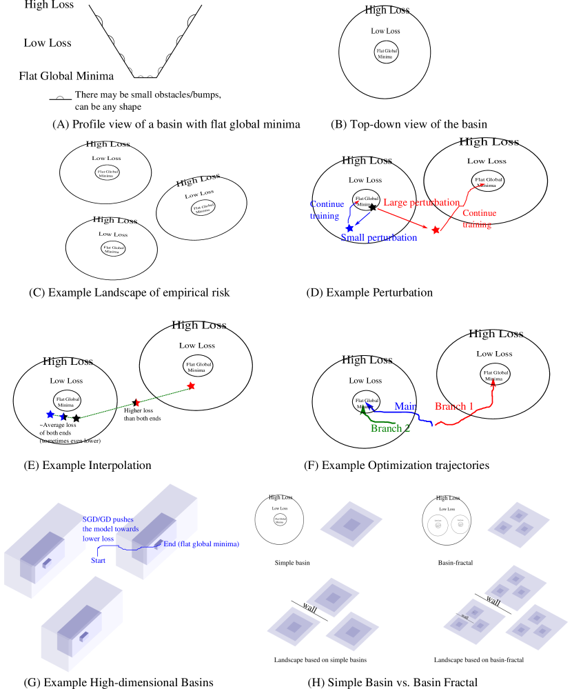
• A simple model of the landscape (Section 5). Summarizing our theoretical and experimental results, we propose a simple baseline model for the landscape of empirical risk, as shown in Figure 1. We conjecture that the loss surface of DCNN is not as complicated as commonly believed. At least in the case of overparametrized DCNNs, the loss surface might be simply a collection of (high-dimensional) basins, which have some of the following interesting properties: 1. Every basin reaches a flat global minima. 2. The basins may be rugged such that any perturbation or noise leads to a slightly different convergence path. 3. Despite being perhaps locally rugged, the basin has a relatively regular overall landscape such that the average of two model within a basin gives a model whose error is roughly the average of (or even lower than) the errors of original two models. 4. Interpolation between basins, on the other hand, may significantly raise the error. 5. There might be some good properties in each basin such that there is no local minima — we do not encounter any local minima in CIFAR, even when training with batch gradient descent without noise.

Figure 1: The Landscape of empirical risk of overparametrized DCNN may be simply a collection of (perhaps slightly rugged) basins. (A) the profile view of a basin (B) the top-down view of a basin (C) example landscape of empirical risk (D) example perturbation: a small perturbation does not move the model out of its current basin, so re-training converges back to the bottom of the same basin. If the perturbation is large, re-training converges to another basin. (E) Example Interpolation: averaging two models within a basin tend to give a error that is the average of the two models (or less). Averaging two models between basins tend to give an error that is higher than both models. (F) Example optimization trajectories that correspond to Figure 4 (G), (H) see Section 5.

2 Framework

We assume a deep network of the convolutional type and overparametrization, that is more weights than data points, since this is how successful deep networks have been used. Under these conditions, we will show that imposing zero empirical error provides a system of equations (at the zeros) that have a large number of degenerate solutions in the weights. The equations are polynomial in the weights, with coefficients reflecting components of the data vectors (one vector per data point). The system of equations is underdetermined (more unknowns than equations, e.g. data points) because of the assumed overparametrization. Because the global minima are degenerate, that is flat in many of the dimensions, they are more likely to be found by SGD than local minima which are less degenerate. Although generalization is not the focus of this work, such flat minima are likely to generalize better than sharp minima, which might be the reason why overparametrized deep networks do not seem to overfit.

3 Landscape of the Empirical Risk: Theoretical Analyses

The following theoretical analysis of the landscape of the empirical risk is based on a few assumptions: (1) We assume that the network is overparametrized, typically using several times more parameters (the weights of the network) than data points. In practice, even with data augmentation (in most of the experiments in this paper we do not use data augmentation), one can always make the model larger to achieve overparametrization without sacrificing either the training or generalization performance. (2) This section assumes a regression framework. We study how many solutions in weights lead to perfect prediction of training labels. In classification settings, such solutions is a subset of all solutions.

Among the critical points of the gradient of the empirical loss, we consider first the zeros of loss function given by the set of equations where $N$ is the number of training examples $f(x_{i})-y_{i}=0\,\,\,\,for\,\,i=1,\cdots,N$

The function $f$ realized by a deep neural network is polynomial if each of RELU units is replaced by a univariate polynomial. Of course each RELU can be approximated within any desired $\epsilon$ in the sup norm by a polynomial. In the well-determined case (as many unknown weights as equations, that is data points), Bezout theorem provides an upper bound on the number of solutions. The number of distinct zeros (counting points at infinity, using projective space, assigning an appropriate multiplicity to each intersection point, and excluding degenerate cases) would be equal to $Z$ - the product of the degrees of each of the equations. Since the system of equations is usually underdetermined – as many equations as data points but more unknowns (the weights) – we expect an infinite number of global minima, under the form of $Z$ regions of zero empirical error. If the equations are inconsistent there are still many global minima of the squared error that are solutions of systems of equations with a similar form.

We assume for simplicity that the equations have a particular compositional form (see [4]). The degree of each approximating equation $\ell^{d}(\epsilon)$ is determined by the desired accuracy $\epsilon$ for approximating the ReLU activation by a univariate polynomial $P$ of degree $\ell(\epsilon)$ and by the number of layers $d$.

The argument based on RELUs approximation for estimating the number of zeros is a qualitative one since good approximation of the $f(x_{i})$ does not imply by itself good approximation – via Bezout theorem – of the number of its zeros. Notice, however, that we could abandon completely the approximation approach and just consider the number of zeros when the RELUs are replaced by a low order univariate polynomial. The argument then would not strctly apply to RELU networks but would still carry weight because the two types of networks – with polynomial activation and with RELUs – behave empirically (see Figure 2) in a similar way.

In the Supporting Material we provide a simple example of a network with associated equations for the exact zeros. They are a system of underconstrained polynomial equations of degree $l^{d}$. In general, there are as many constraints as data points $i=1,\cdots,N$ for a much larger number $K$ of unknown weights $W,w,\cdots$. There are no solutions if the system is inconsistent – which happens if and only if $0=1$ is a linear combination (with polynomial coefficients) of the equations (this is Hilbert’s Nullstellensatz). Otherwise, it has infinitely many complex solutions: the set of all solutions is an algebraic set of dimension at least $K-N$. If the underdetermined system is chosen at random the dimension is equal to $K-N$ with probability one.

Even in the non-degenerate case (as many data as parameters), Bezout theorem suggests that there are many solutions. With $d$ layers the degree of the polynomial equations is $\ell^{d}$. With $N$ datapoints the Bezout upper bound in the zeros of the weights is $\ell^{Nd}$. Even if the number of real zero – corresponding to zero empirical error – is much smaller (Smale and Shub estimate [5] $l^{\frac{Nd}{2}}$), the number is still enormous: for a CiFAR situation this may be as high as $2^{10^{5}}$.

As mentioned, in several cases we expect absolute zeros to exist with zero empirical error. If the equations are inconsistent it seems likely that global minima with similar properties exist.

It is interesting now to consider the critical points of the gradient. The critical points of the gradient are $\nabla_{w}\sum_{i=1}^{N}V(f(x_{i}),y_{i})=0$, which gives $K$ equations: $\sum_{i=1}^{N}\nabla_{w}V(f(x_{i}),y_{i})\nabla_{w}f(x_{i})=0$, where $V(.,.)$ is the loss function.

Approximating within $\epsilon$ in the sup norm each ReLU in $f(x_{i})$ with a fixed polynomial $P(z)$ yields again a system of $K$ polynomial equations in the weights of higher order than in the case of zero-minimizers. They are of course satisfied by the degenerate zeros of the empirical error but also by additional non-degenerate (in the general case) solutions.

Thus, we have Proposition 1: There are a very large number of zero-error minima which are highly degenerate unlike the local non-zero minima.

4 The Landscape of the Empirical Risk: Visualizing and Analysing the Loss Surface During the Entire Training Process (on CIFAR-10)

4.1 Experimental Settings

In the empirical work described below we analyze a classification problem with cross entropy loss. Our theoretical analyses with the regression framework provide a lower bound of the number of solutions of the classification problem.

Unless mentioned otherwise, we trained a 6-layer (with the 1st layer being the input) Deep Convolutional Neural Network (DCNN) on CIFAR-10. All the layers are 3x3 convolutional layers with stride 2. No pooling is performed. Batch Normalizations (BNs) [6] are used between hidden layers. The shifting and scaling parameters in BNs are not used. No data augmentation is performed, so that the training set is fixed (size = 50,000). There are 188,810 parameters in the DCNN.

Multidimensional Scaling The core of our visualization approach is Multidimensional Scaling (MDS) [7]. We record a large number of intermediate models during the process of several training schemes. Each model is a high dimensional point with the number of dimensions being the number of parameters. The strain-based MDS algorithm is applied to such points and a corresponding set of 2D points are found such that the dissimilarity matrix between the 2D points are as similar to those of the high-dimensional points as possible. One minus cosine distance is used as the dissimilarity metric. This is more robust to scaling of the weights, which is usually normalized out by BNs. Euclidean distance gives qualitatively similar results though.

Figure 2: One can convert a deep network into a polynomial function by using polynomial nonlinearity. As long as the nonlinearity approximates ReLU well (especially near 0), the “polynomial net” performs similarly to a ReLU net. Our theory applies rigorously to a “polynomial net”.

4.2 Global Visualization of SGD Training Trajectories

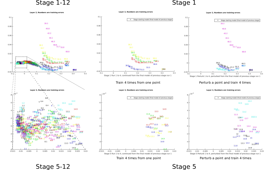
We show in Figure 3 the optimization trajectories of Stochastic Gradient Descent (SGD) throughout the entire optimization process of training a DCNN on CIFAR-10. The SGD trajectories follow the mini-batch approximations of the training loss surface. Although the trajectories are noisy due to SGD, the collected points along the trajectories provide a good visualization of the landscape of empirical risk. We show the visualization based on the weights of layer 2. The results from other layers (e.g., layer 5) are qualitatively similar and are shown in the Appendix.

Figure 3: We train a 6-layer (with the 1st layer being the input) convolutional network on CIFAR-10 with stochastic gradient descent (batch size = 100). We divide the training process into 12 stages. In each stage, we perform 8 parallel SGDs with learning rate 0.01 for 10 epochs, resulting in 8 parallel trajectories denoted by different colors. Trajectories 1 to 4 in each stage start from the final model (denoted by $P$) of trajectory 1 of the previous stage. Trajectories 5 to 8 in each stage start from a perturbed version of $P$. The perturbation is performed by adding a gaussian noise to the weights of each layer with the standard deviation being 0.01 times layer’s standard deviation. In general, we observe that running any trajectory with SGD again almost always leads to a slightly different convergence path. We plot the MDS results of all the layer 2 weights collected throughout all the training epochs from stage 1 to 12. Each number in the figure represents a model we collected during the above procedures. The points are in a 2D space generated by the MDS algorithm such that their pairwise distances are optimized to try to reflect those distances in the original high-dimensional space. The results of stages more than 5 are quite cluttered. So we applied a separate MDS to the stages 5 to 12. We also plot stage 1 and 5 separately for example. The trajectories of more stages are plotted in the Appendix.

4.3 Global Visualization of Training Loss Surface with Batch Gradient Descent

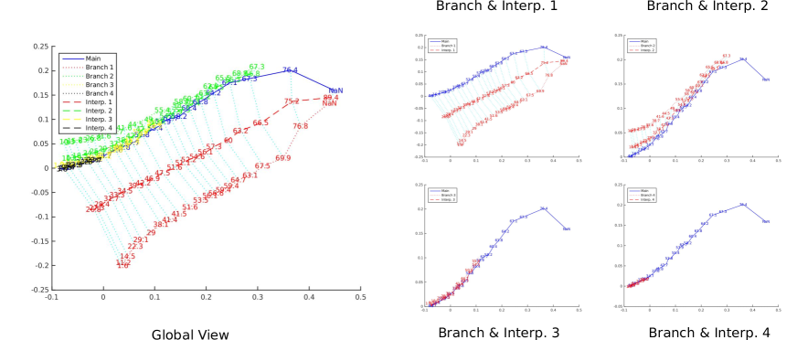
Next, we visualize in Figure 4 the exact training loss surface by training the models using Batch Gradient Descent (BGD). In addition to training, we also performed perterbation and interpolation experiments as described in Figure 4. The main trajectory, branches and the interpolated models together provides a good visualization of the landscape of the empirical risk.

Figure 4: Visualizing the exact training loss surface using Batch Gradient Descent (BGD). A DCNN is trained on CIFAR-10 from scratch using Batch Gradient Descent (BGD). The numbers are training errors. “NaN” corresponds to randomly initialized models (we did not evaluate them and assume they perform at chance). At epoch 0, 10, 50 and 200, we create a branch by perturbing the model by adding a Gaussian noise to all layers. The standard deviation of the Gaussian is 0.25*S, where S denotes the standard deviation of the weights in each layer, respectively. We also interpolate (by averaging) the models between the branches and the main trajectory, epoch by epoch. The interpolated models are evaluated on the entire training set to get a performance. First, surprisingly, BGD does not get stuck in any local minima, indicating some good properties of the landscape. The test error of solutions found by BGD is somewhat worse than those found by SGD, but not too much worse (BGD   40%, SGD   32%) . Another interesting observation is that as training proceeds, the same amount of perturbation are less able to lead to a drastically different trajectory. Nevertheless, a perturbation almost always leads to at least a slightly different model. The local neighborhood of the main trajectory seems to be relatively flat and contain many good solutions, supporting our theoretical predictions. It is also intriguing to see interpolated models to have very reasonable performance. The results here are based on weights from layer 2. The results of other layers are similar and are shown in the Appendix.

4.4 More Detailed Analyses of Several Local Landscapes (especially the flat global minima)

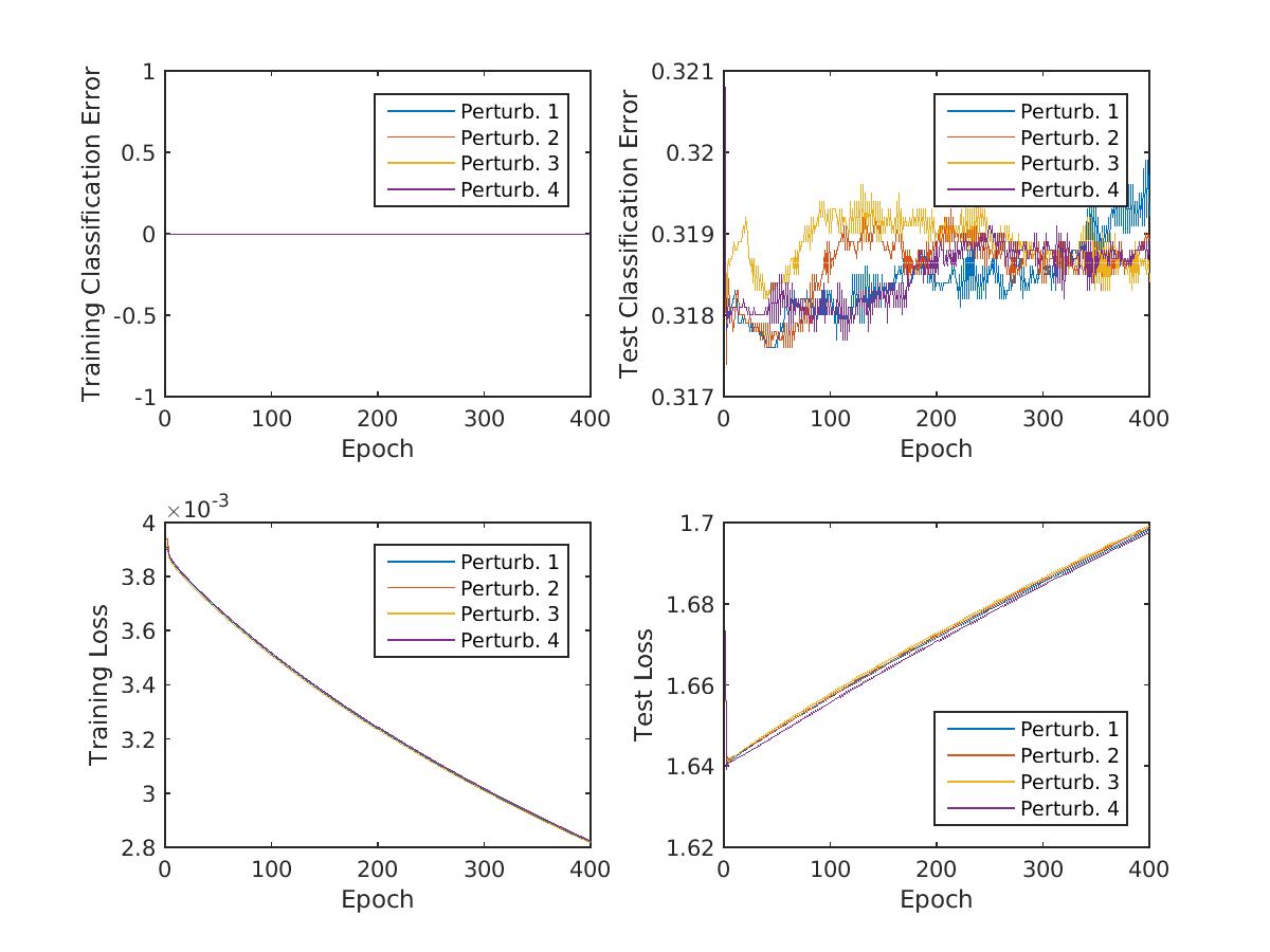
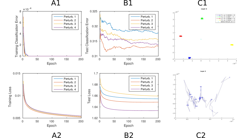
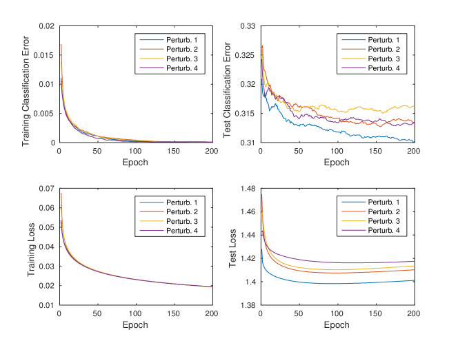
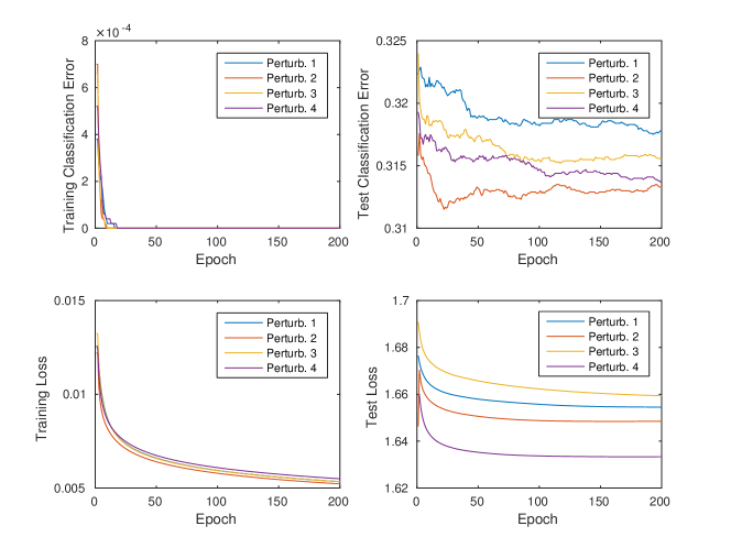
We perform some more detailed analyses at several locations of the landscape. Especially, we would like to check if the global minima is flat. We train a 6-layer (with the 1st layer being the input) DCNN on CIFAR-10 with 60 epochs of SGD (batch size = 100) and 400 epochs of Batch Gradient Descent (BGD). BGD is performed to get to as close to the global minima as possible. Next we select three models from this learning trajectory (1) $M_{5}$: the model at SGD epoch 5. (2) $M_{30}$: the model at SGD epoch 30. (3) $M_{final}$: the final model after 60 epochs of SGD and 400 epochs of BGD. The results of (3) are shown in Figure 5 while those of (1) and (2) are shown in the the Appendix.

Figure 5: Verifying the flatness of global minima: We layerwise perturb the weights of model $M_{final}$ (which is at a global minimum) by adding a gaussian noise with standard deviation = 0.1 * S, where S is the standard deviation of the weights. After perturbation, we continue training the model with 200 epochs of gradient descent (i.e., batch size = training set size). The same procedure was performed 4 times, resulting in 4 curves shown in the figures. The training and test classification errors and losses are shown in A1, A2, B1 and B2. The MDS visualization of 4 trajectories (denoted by 4 colors) is shown in C1 — the 4 trajectories converge to different solutions. The MDS visualization of one trajectory is in C2. In addition, we show the confusion matrices of converged models in the Appendix to verify that they are indeed different models. More similar experiments can be found in the Appendix.

5 The Landscape of the Empirical Risk: Towards an Intuitive Baseline Model

In this section, we propose a simple baseline model for the landscape of empirical risk that is consistent with all of our theoretical and experimental findings. In the case of overparametrized DCNNs, here is a recapitulation of our main observations:
$\bullet$ Theoretically, we show that there are a large number of global minimizers with zero (or small) empirical error. The same minimizers are degenerate.
$\bullet$ Regardless of Stochastic Gradient Descent (SGD) or Batch Gradient Descent (BGD), a small perturbation of the model almost always leads to a slightly different convergence path. The earlier the perturbation is in the training process the more different the final model would be.
$\bullet$ Interpolating two “nearby” convergence paths lead to another convergence path with similar errors every epoch. Interpolating two “distant” models lead to raised errors.
$\bullet$ We do not observe local minima, even when training with BGD.

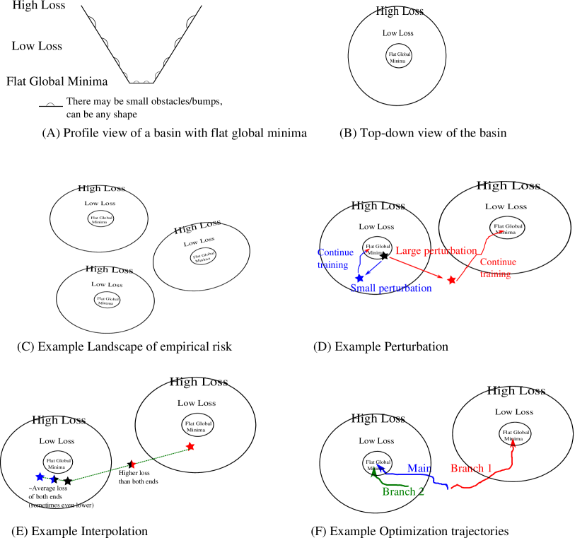
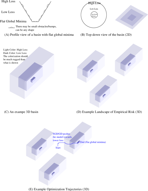
There is a simple model that is consistent with above observations. As a first-order characterization, we believe that the landscape of empirical risk is simply a collection of (hyper) basins that each has a flat global minima. Illustrations are provided in Figure 1.

As shown in Figure 1, the building block of the landscape is a basin. How does a basin look like in high dimension? Is there any evidence for this model? One definition of a hyper-basin would be that as loss decreases, the hypervolume of the parameter space decreases (see Figure 1 (H) for example). As we can see, with the same amount of scaling in each dimension, the volume shrinks much faster as the number of dimension increases — with a linear decrease in each dimension, the hypervolume decreases as a exponential function of the number of dimensions. With the number of dimensions being the number of parameters, the volume shrinks incredibly fast. This leads to a phenomenon that we all observe experimentally: whenever one perturb a model by adding some significant noise, the loss almost always never go down. The larger the perturbation is, the more the error increases. The reasons are simple if the local landscape is a hyper-basin: the volume of a lower loss area is so small that by randomly perturbing the point, there is almost no chance getting there. The larger the perturbation is, the more likely it will get to a much higher loss area.

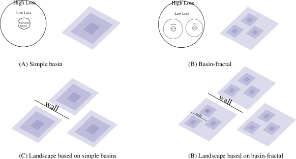
There are, nevertheless, other plausible variants of this model that can explain our experimental findings. In Figure 1 (G), we show one alternative model we call “basin-fractal”. This model is more elegant while being also consistent with most of the above observations. The key difference between simple basins and “basin-fractal” is that in “basin-fractal”, one should be able to find “walls” (raised errors) between two models within the same basin. Since it is a fractal, these “walls” should be present at all levels of errors. For the moment, we only discovered “walls” between two models the trajectories lead to which are very different (obtained either by splitting very early in training, as shown in Figure 4 branch 1 or by a very significant perturbation, as shown in the Appendix). We have not found other significant “walls” in all other perturbation and interpolation experiments. So a first order model of the landscape would be just a collection of simple basins. Nevertheless, we do find “basin-fractal” elegant, and perhaps the “walls” in the low loss areas are just too flat to be noticed.

Another surprising finding about the basins is that, they seem to be so “smooth” such that there is no local minima. Even when training with batch gradient descent, we do not encounter any local minima. When trained long enough with small enough learning rates, one always gets to 0 classification error and negligible cross entropy loss.

6 Previous theoretical work

Deep Learning references start with Hinton’s backpropagation and with LeCun’s convolutional networks (see for a nice review [8]). Of course, multilayer convolutional networks have been around at least as far back as the optical processing era of the 70s. The Neocognitron[9] was a convolutional neural network that was trained to recognize characters. The property of compositionality was a main motivation for hierarchical models of visual cortex such as HMAX which can be regarded as a pyramid of AND and OR layers[10], that is a sequence of conjunctions and disjunctions. [3] provided formal conditions under which deep networks can avoid the curse of dimensionality. More specifically, several papers have appeared on the landscape of the training error for deep networks. Techniques borrowed from the physics of spin glasses (which in turn were based on old work by Marc Kac on the zeros of algebraic equations) were used [11] to suggest the existence of a band of local minima of high quality as measured by the test error. The argument however depends on a number of assumptions which are rather implausible (see [12] and [13] for comments and further work on the problem). Soudry and Carmon [12] show that with mild over-parameterization and dropout-like noise, training error for a neural network with one hidden layer and piece-wise linear activation is zero at every local minimum. All these results suggest that the energy landscape of deep neural networks should be easy to optimize. They more or less hold in practice —it is easy to optimize a prototypical deep network to near-zero loss on the training set.

7 Discussion and Conclusions

Are the results shown in this work data dependent? We visualized the SGD trajectories in the case of fitting random labels. There is no qualitative difference between the results from those of normal labels. So it is safe to say the results are at least not label dependent. We will further check if fitting random input data to random labels will give similar results.
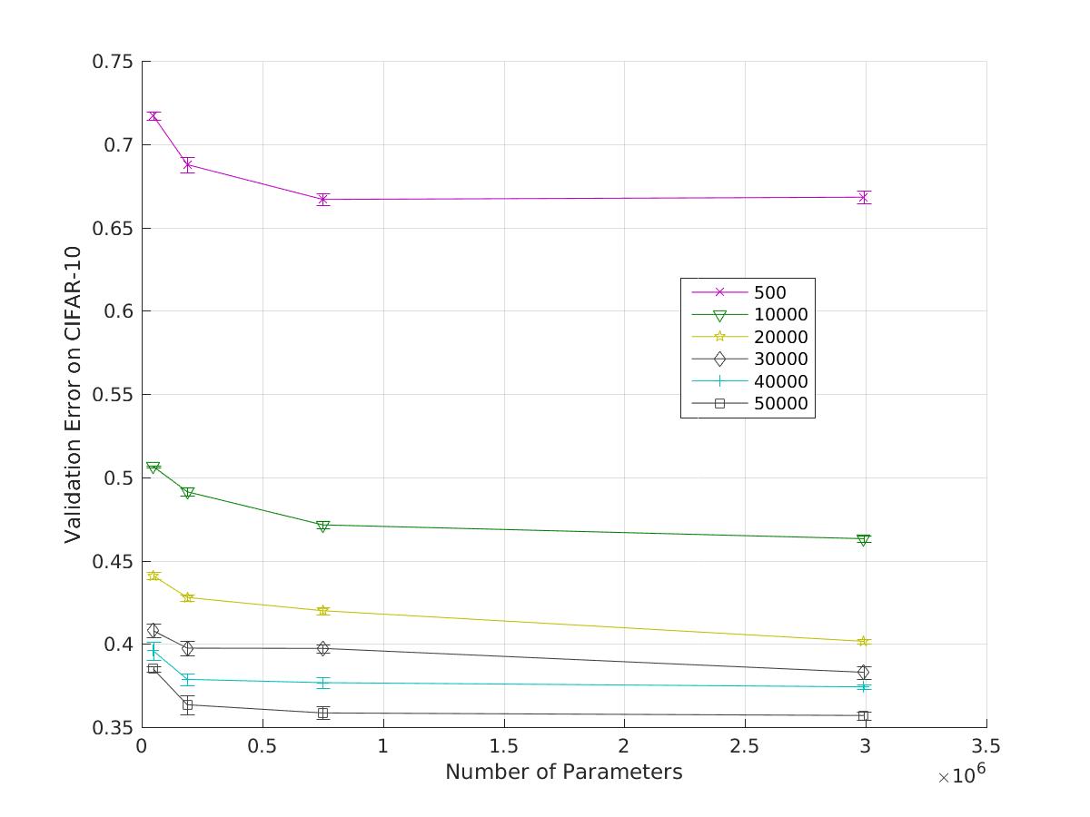
What about Generalization? It is experimentally observed that (see Figure 40 in the Appendix), at least in all our experiments, overparametrization (e.g., 60x more parameters than data) does not hurt generalization at all.
Conclusions: Overall, we characterize the landscape of empirical risk of overparametrized DCNNs with a mix of theoretical analyses and experimental explorations. We provide a simple baseline model of the landscape that can account for all of our theoretical and experimental results. Nevertheless, as the final model is so simple, it is hard to believe that it would completely characterize the true loss surface of DCNN. Further research is warranted.

Figure 6: The Landscape of empirical risk of overparametrized DCNN may be simply a collection of (perhaps slightly rugged) basins. (A) the profile view of a basin (B) the top-down view of a basin (C) example landscape of empirical risk (D) example perturbation: a small perturbation does not move the model out of its current basin, so re-training converges back to the bottom of the same basin. If the perturbation is large, re-training converges to another basin. (E) Example Interpolation: averaging two models within a basin tend to give a error that is the average of the two models (or less). Averaging two models between basins tend to give an error that is higher than both models. (F) Example optimization trajectories that correspond to Figure 14 and Figure 16.

Appendix A Landscape of the Empirical Risk: Theoretical Analyses

A.1 Optimization of compositional functions: Bezout theorem

The following analysis of the landscape of the empirical risk is based on two assumptions that hold true in most applications of deep convolutional networks:

1. overparametrization of the network, typically using several times more parameters (the weights of the network) than data points. In practice, even with data augmentation, one can always make the model larger to achieve overparametrization without sacrificing either the training or generalization performance.

2. each of the equations corresponding to zeros of the empirical risk (we assume a regression framework attempting to minimize a loss such as square loss) can be approximated by a polynomial equation in the weights, by a polynomial approximaton within $\epsilon$ (in the sup norm) of the RELU nonlinearity.

The main observation is that the degree of each approximating equation $\ell^{d}(\epsilon)$ is determined by the accuracy $\epsilon$ we desire for approximating the ReLU activation by a univariate polynomial $P$ of degree $\ell(\epsilon)$ and by the number of layers $d$. This approximation argument is of course a qualitative one sice good approximation of the function does not imply by itself good approximation of the number of its zeros. Notice that we could abandon completely the approximation approach and just consider the number of zeros when the RELUs are exactly a low order univariate polinomial. The argument then would not apply to RELU networks but would still carry weight because the two types of networks – with polynomial activation and with RELUs – behave theoretically (see ) and empirically in a similar way. In the well-determined case (as many unknown weights as equations, that is data points), Bezout theorem provides an upper bound on the number of solutions. The number of distinct zeros (counting points at infinity, using projective space, assigning an appropriate multiplicity to each intersection point, and excluding degenerate cases) would be equal to $Z$ - the product of the degrees of each of the equations. Since the system of equations is usually underdetermined – as many equations as data points but more unknowns (the weights) – we expect an infinite number of global minima, under the form of $Z$ regions of zero empirical error. If the equations are inconsistent there are still many global minima of the squared error that is solutions of systems of equations with a similar form.

A.2 Global minima with zero error

We consider a simple example in which the zeros of the empirical error (that is exact solutions of the set of equations obtained by setting $f(x^{i})-y_{i}=0$, where $i=1,\cdots,N$ are the data points and $f(x)$ is the network parametrized by weights $w$). In particular, we consider the zeros on the training set of a network with ReLUs activation approximating a function of four variables with the following structure:

$$f(x_{1},x_{2},x_{3},x_{4})=g(h(x_{1},x_{2}),h^{\prime}(x_{3},x_{4})).$$ (1)

We assume that the deep approximation network uses ReLUs as follows

$$g(h,h)=A(W_{1}h+W_{2}h+W_{3})_{+}+B(W^{\prime}_{1}h+W^{\prime}_{2}h+W^{\prime}_{3})_{+}$$ (2)

and

$$h(x_{1},x_{2})=a(w_{1}x_{1}+w_{2}x_{2}+w_{3})_{+}+b(v_{1}x_{1}+v_{2}x_{2}+v_{3})_{+},$$ (3)

$$h^{\prime}(x_{3},x_{4})=a^{\prime}(w^{\prime}_{1}x_{1}+w^{\prime}_{2}x_{2}+w^{\prime}_{3})_{+}+b^{\prime}(v_{1}^{\prime}x_{1}+v_{2}^{\prime}x_{2}+v_{3}^{\prime})_{+}.$$ (4)

There are usually quite a few more units in the first and second layer than the $2$ of the example above.

This example generalizes to the case in which the kernel support is larger than $2$ (for instance is $3x3=9$ as in ResNets). In the standard case each node (for instance in the first layer) contains quite a few units ($O(100)$) and as many outputs. However, the effective outputs are much fewer so that each is the linear combination of several ReLUs units.

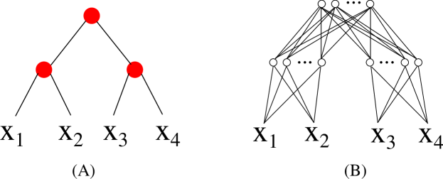
Consider Figure 7. The approximating polynomial equations for the zero of the empirical errors for this network, which could be part of a larger network, are, for $i=1,\cdots,N$ where $N$ are the data points:

$$P(W_{1}P(w_{1}x_{i,1}+w_{2}x_{i,2}+w_{3})+W_{2}P(w_{1}x_{i,3}+w_{2}x_{i,4}+w_{3})+$$ (5)

$$+W_{3})-y_{i}=0$$ (6)

The above equations describe the simple case of one ReLU per node for the case of the network of Figure 7. Equations 5 are a system of underconstrained polynomial equations of degree $l^{d}$. In general, there are as many constraints as data points $i=1,\cdots,N$ for a much larger number $K$ of unknown weights $W,w,\cdots$. There are no solutions if the system is inconsistent – which happens if and only if $0=1$ is a linear combination (with polynomial coefficients) of the equations (this is Hilbert’s Nullstellensatz). Otherwise, it has infinitely many complex solutions: the set of all solutions is an algebraic set of dimension at least $K-N$. If the underdetermined system is chosen at random the dimension is equal to $K-N$ with probability one.

Figure 7: The diagram (B) shows a 3 nodes part of a network; the corresponding compositional function of the form $f(x_{1},\cdots,x_{4})=h_{2}(h_{11}(x_{1},x_{2}),h_{12}(x_{3},x_{4}))$ represented by the binary graph (A). In the approximating network each of the $3$ nodes in the graph corresponds to a set of $Q$ ReLU units computing the ridge function $\sum_{i=1}^{Q}a_{i}(\left\langle{\mathbf{v}_{i}},{\mathbf{x}}\right\rangle+t_{i})_{+}$, with $\mathbf{v}_{i},\mathbf{x}\in\operatorname{\mathbb{R}}^{2}$, $a_{i},t_{i}\in\operatorname{\mathbb{R}}$. Corollary LABEL:appendix:rank implies that in a network that has a consistent accuracy across the layers the matrix of the weights to the top node should have a rank in the order of the number of inputs of the connected nodes at the lower layer: in this case the rank is $4$.

Even in the non-degenerate case (as many data as parameters), Bezout theorem suggests that there are many solutions. With $d$ layers the degree of the polynomial equations is $\ell^{d}$. With $N$ datapoints the Bezout upper bound in the zeros of the weights is $\ell^{Nd}$. Even if the number of real zero – corresponding to zero empirical error – is much smaller (Smale and Shub estimate [5] $l^{\frac{Nd}{2}}$), the number is still enormous: for a CiFAR situation this may be as high as $2^{10^{5}}$.

A.3 Minima

As mentioned, in several cases we expect absolute zeros to exist with zero empirical error. If the equations are inconsistent it seems likely that global minima with similar properties exist.

Corollary 1

In general, non-zero minima exist with higher dimensionality than the zero-error global minima: their dimensionality is the number of weights $K$ vs. the number of data points $N$. This is true in the linear case and also in the presence of ReLUs.

Let us consider the same example as before looking at the critical points of the gradient. With a square loss function the critical points of the gradient are:

$$\nabla_{w}\sum_{i=1}^{N}(f(x_{i})-y_{i})^{2}=0$$ (7)

which gives $K$ equations

$$\sum_{i=1}^{N}(f(x_{i})-y_{i})\nabla_{w}f(x_{i})=0.$$ (8)

Approximating within $\epsilon$ in the sup norm each ReLU in $f(x_{i})$ with a fixed polynomial $P(z)$ yields again a system of $K$ polynomial equations in the weights of higher order than in the case of zero-minimizers. They are of course satisfied by the degenerate zeros of the empirical error but also by additional non-degenerate (in the general case) solutions.

We summarize our main observations on the $\epsilon$ approximating system of equations in the following

Proposition 1

There are a very large number of zero-error minima which are highly degenerate unlike the local non-zero minima.

Appendix B The Landscape of the Empirical Risk: Visualizing and Analysing the Loss Surface During the Entire Training Process (on CIFAR-10)

In the empirical work described below we analyze a classification problem with cross entropy loss. Our theoretical analyses with the regression framework provide a lower bound of the number of solutions of the classification problem.

B.1 Experimental Settings

Unless mentioned otherwise, we trained a 6-layer (with the 1st layer being the input) Deep Convolutional Neural Network (DCNN) on CIFAR-10. All the layers are 3x3 convolutional layers with stride 2. No pooling is performed. Batch Normalizations (BNs) are used between hidden layers. The shifting and scaling parameters in BNs are not used. No data augmentation is performed, so that the training set is fixed (size = 50,000). There are 188,810 parameters in the DCNN.

Multidimensional Scaling The core of our visualization approach is Multidimensional Scaling (MDS) [7]. We record a large number of intermediate models during the process of several training schemes. Each model is a high dimensional point with the number of dimensions being the number of parameters. The strain-based MDS algorithm is applied to such points and a corresponding set of 2D points are found such that the dissimilarity matrix between the 2D points are as similar to those of the high-dimensional points as possible. One minus cosine distance is used as the dissimilarity metric. This is more robust to scaling of the weights, which is usually normalized out by BNs. Euclidean distance gives qualitatively similar results though.

B.2 Global Visualization of SGD Training Trajectories

We show the optimization trajectories of Stochastic Gradient Descent (SGD), since this is what people use in practice. The SGD trajectories follow the mini-batch approximations of the training loss surface. Although the trajectories are noisy due to SGD, the collected points along the trajectories provide a visualization of the landscape of empirical risk.

We train a 6-layer (with the 1st layer being the input) convolutional network on CIFAR-10 with stochastic gradient descent (batch size = 100) We divide the training process into 12 stages. In each stage, we perform 8 parallel SGDs with learning rate 0.01 for 10 epochs, resulting in 8 parallel trajectories denoted by different colors in each subfigure of Figure 9 and 11. Trajectories 1 to 4 in each stage start from the final model (denoted by $P$) of trajectory 1 of the previous stage. Trajectories 5 to 8 in each stage start from a perturbed version of $P$. The perturbation is performed by adding a gaussian noise to the weights of each layer with the standard deviation being 0.01 times layer’s standard deviation. In general, we observe that running any trajectory with SGD again almost always leads to a slightly different model.

Taking layer 2 weights for example, we plot the global MDS results of stage 1 to 12 in Figure 8. The detailed parallel trajectories of stage 1 to 3 are plotted separately in Figure 9.

The results of stages more than 5 are quite cluttered. So we applied a separate MDS to the stages 5 to 12 and show the results in Figure 10. The detailed parallel trajectories of stage 5 to 7 are plotted separately in Figure 11.

The weights of different layers tend to produce qualitatively similar results. We show the results of layer 5 in Figure 12 and Figure 13.

Figure 8: Training a DCNN on CIFAR-10. We divide the training process into 12 stages. In each stage, we perform 8 parallel SGDs with learning rate 0.01 for 10 epochs, resulting in 8 parallel trajectories denoted by different colors. Trajectories 1 to 4 in each stage start from the final model (denoted by $P$) of trajectory 1 of the previous stage. Trajectories 5 to 8 in each stage start from a perturbed version of $P$. The perturbation is performed by adding a gaussian noise to the weights of each layer with the standard deviation being 0.01 times layer’s standard deviation. In general, we observe that running any trajectory with SGD again almost always leads to a slightly different convergence path. We plot the MDS results of all the layer 2 weights collected throughout all the training epochs from stage 1 to 12. The detailed parallel trajectories of stage 1 to 3 are plotted separately in Figure 9. Each number in the figure represents a model we collected during the above procedures. The points are in a 2D space generated by the MDS algorithm such that their pairwise distances are optimized to try to reflect those distances in the original high-dimensional space. The results of stages more than 5 are quite cluttered. So we applied a separate MDS to the stages 5 to 12 and show the results in Figure 10. The detailed parallel trajectories of stage 5 to 7 are plotted separately in Figure 11.

(a) In stage 1, the starting model is the randomly initialized model.

(b)

(c)

(d)

(e)

(f)

Figure 9: Parallel trajectories from stage 1 to 3 of Figure 8 are plotted separately. More details are described in Figure 8

Figure 10: A separate MDS performed on stage 5 to 12 of Figure 8 to provide more resolution. Details are described in the caption of Figure 8

(a)

(b)

(c)

(d)

(e)

(f)

Figure 11: Parallel trajectories from stage 5 to 7 of Figure 8 are plotted separately. More details are described in Figure 8

Figure 12: Same as Figure 8, but all weights are collected from Layer 5.

Figure 13: Same as Figure 10, but all weights are collected from Layer 5.

B.3 Global Visualization of Training Loss Surface with Batch Gradient Descent

Next, we visualize the exact training loss surface by training the models using Batch Gradient Descent (BGD). We adopt the following procedures: We train a model from scratch using BGD. At epoch 0, 10, 50 and 200, we create a branch by perturbing the model by adding a Gaussian noise to all layers. The standard deviation of the Gaussian noise is a meta parameter, and we tried 0.25*S, 0.5*S and 1*S, where S denotes the standard deviation of the weights in each layer, respectively.

We also interpolate (by averaging) the models between the branches and the main trajectory, epoch by epoch. The interpolated models are evaluated on the entire training set to get a performance (in terms of error percentage).

The main trajectory, branches and the interpolated models together provides a good visualization of the landscape of the empirical risk.

Figure 14: The 2D visualization using MDS of weights in layer 2. A DCNN is trained on CIFAR-10 from scratch using Batch Gradient Descent (BGD). The numbers are training errors. “NaN” corresponds to randomly initialized models (we did not evaluate them and assume they perform at chance). At epoch 0, 10, 50 and 200, we create a branch by perturbing the model by adding a Gaussian noise to all layers. The standard deviation of the Gaussian is 0.25*S, where S denotes the standard deviation of the weights in each layer, respectively. We also interpolate (by averaging) the models between the branches and the main trajectory, epoch by epoch. The interpolated models are evaluated on the entire training set to get a performance. First, surprisingly, BGD does not get stuck in any local minima, indicating some good properties of the landscape. The test error of solutions found by BGD is somewhat worse than those found by SGD, but not too much worse (BGD   40%, SGD   32%) . Another interesting observation is that as training proceeds, the same amount of perturbation are less able to lead to a drastically different trajectory. Nevertheless, a perturbation almost always leads to at least a slightly different model. The local neighborhood of the main trajectory seems to be relatively flat and contain many good solutions, supporting our theoretical predictions. It is also intriguing to see interpolated models to have very reasonable performance.

(a)

(b)

(c)

(d)

Figure 15: Same as Figure 14, but 4 branches are plotted separately to avoid clutter.

Figure 16: Same as Figure 14 except: (1) the weights of layer 3 are visualized, instead of layer 2. (2) the perturbation is significantly larger: we create a branch by perturbing the model by adding a Gaussian noise to all layers. The standard deviation of the Gaussian is S, where S denotes the standard deviation of the weights in each layer, respectively. Larger perturbations leads to more separated branches.

(a)

(b)

(c)

(d)

Figure 17: Same as Figure 16, but 4 branches are plotted separately to avoid clutter. Compared to Figure 15, here we have larger perturbations when creating a branch, which leads to more separated trajectories (e.g., subfigure (b)).

B.4 More Detailed Analyses of Several Local Landscapes (especially the flat global minima)

After the global visualization of the loss surface, we perform some more detailed analyses at several locations of the landscape. Especially, we would like to check if the global minima is flat. We train a 6-layer (with the 1st layer being the input) DCNN on CIFAR-10 with 60 epochs of SGD (batch size = 100) and 400 epochs of Batch Gradient Descent (BGD). BGD is performed to get to as close to the global minima as possible.

Next we select three models from this learning trajectory

• $M_{5}$: the model at SGD epoch 5.

• $M_{30}$: the model at SGD epoch 30.

• $M_{final}$: the final model after 60 epochs of SGD and 400 epochs of BGD.

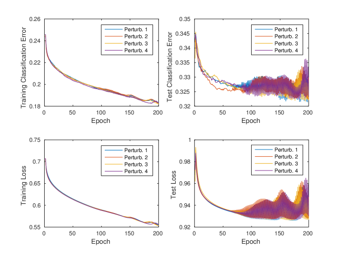
We perturb the weights of these models and retrain them with BGD, respectively. This procedure was done multiple times for each model to get an idea of the nearby empirical risk landscape.

The results are consistent with the previous theoretical arguments:

• global minima are easily found with zero classification error and negligible cross entropy loss.

• The global minima seem “flat” under perturbations with zero error corresponding to different parameters values.

• The local landscapes at different levels of error seem to be very similar. Perturbing a model always lead to a different convergence path, leading to a similar but distinct model. We tried smaller perturbations and also observed this effect.

B.4.1 Perturbing the model at SGD Epoch 5

Figure 18: We layerwise perturb the weights of model $M_{5}$ by adding a gaussian noise with standard deviation = 0.1 * S, where S is the standard deviation of the weights. After perturbation, we continue training the model with 200 epochs of gradient descent (i.e., batch size = training set size). The same procedure was performed 4 times, resulting in 4 curves shown in the figures. The training and test classification errors and losses are shown.

Figure 19: Multidimensional scaling of the layer 2 weights throughout the retraining process. There are 4 runs indicated by 4 colors/trajectories, corresponding exactly to Figure 41. Each run corresponds to one perturbation of the model $M_{5}$ and subsequent 200 epochs’ training. The number in the figure indicates the training epoch number after the initial perturbation.

Figure 20: Multidimensional scaling of the layer 4 weights throughout the training process. There are 4 runs indicated by 4 colors/trajectories, corresponding exactly to Figure 41. Each run corresponds to one perturbation of the model $M_{5}$ and subsequent 200 epochs’ training. The number in the figure indicates the training epoch number after the initial perturbation.

Figure 21: Multidimensional scaling of the layer 6 weights throughout the training process. There are 4 runs indicated by 4 colors/trajectories, corresponding exactly to Figure 41. Each run corresponds to one perturbation of the model $M_{5}$ and subsequent 200 epochs’ training. The number in the figure indicates the training epoch number after the initial perturbation.

(a)

(b)

(c)

Figure 22: The Multidimensional Scaling (MDS) of the layer 2/4/6 weights of model $M_{5}$ throughout the retraining process. Only the weights of one run (run 1 in Figure 41) are fed into MDS to provide more resolution. The number in the figure indicates the training epoch number after the initial perturbation.

Figure 23: The similarity between the final models of the 4 perturbations (row/column 1-4) of $M_{5}$ and a random reference model (the 5-th row/column). The left figure shows the probability of the column model being correct given the row model is correct. The right figure shows the probability of the column model being incorrect given the row model is incorrect. These two figures show that the perturbed models really become different (although a little similar) models after continued training.

B.4.2 Perturbing the model at SGD Epoch 30

Figure 24: We layerwise perturb the weights of model $M_{30}$ by adding a gaussian noise with standard deviation = 0.1 * S, where S is the standard deviation of the weights. After perturbation, we continue training the model with 200 epochs of gradient descent (i.e., batch size = training set size). The same procedure was performed 4 times, resulting in 4 curves shown in the figures. The training and test classification errors and losses are shown.

Figure 25: Multidimensional scaling of the layer 2 weights throughout the retraining process. There are 4 runs indicated by 4 colors/trajectories, corresponding exactly to Figure 41. Each run corresponds to one perturbation of the model $M_{30}$ and subsequent 200 epochs’ training. The number in the figure indicates the training epoch number after the initial perturbation.

Figure 26: Multidimensional scaling of the layer 4 weights throughout the training process. There are 4 runs indicated by 4 colors/trajectories, corresponding exactly to Figure 41. Each run corresponds to one perturbation of the model $M_{30}$ and subsequent 200 epochs’ training. The number in the figure indicates the training epoch number after the initial perturbation.

Figure 27: Multidimensional scaling of the layer 6 weights throughout the training process. There are 4 runs indicated by 4 colors/trajectories, corresponding exactly to Figure 41. Each run corresponds to one perturbation of the model $M_{30}$ and subsequent 200 epochs’ training. The number in the figure indicates the training epoch number after the initial perturbation.

(a)

(b)

(c)

Figure 28: The Multidimensional Scaling (MDS) of the layer 2/4/6 weights of model $M_{30}$ throughout the retraining process. Only the weights of one run (run 1 in Figure 41) are fed into MDS to provide more resolution. The number in the figure indicates the training epoch number after the initial perturbation.

Figure 29: The similarity between the final models of the 4 perturbations (row/column 1-4) of $M_{30}$ and a random reference model (the 5-th row/column). The left figure shows the probability of the column model being correct given the row model is correct. The right figure shows the probability of the column model being incorrect given the row model is incorrect. These two figures show that the perturbed models really become different (although a little similar) models after continued training.

Figure 30: Interpolating perturbation 1 and 2 of $M_{30}$. The top and bottom rows interpolate the perturbed models before and after retraining, respectively. The x axes are interpolating ratios — at x=0 the model becomes perturbed model 1 and at x=1 the model becomes perturbed model 2. It is a little surprising to find that the interpolated models between perturbation 1 and 2 can even have slightly lower errors. Note that this is no longer the case if the perturbations are very large.

B.4.3 Perturbing the final model (SGD 60 + GD 400 epochs)

Figure 31: We layerwise perturb the weights of model $M_{final}$ by adding a gaussian noise with standard deviation = 0.1 * S, where S is the standard deviation of the weights. After perturbation, we continue training the model with 200 epochs of gradient descent (i.e., batch size = training set size). The same procedure was performed 4 times, resulting in 4 curves shown in the figures. The training and test classification errors and losses are shown.

Figure 32: Multidimensional scaling of the layer 2 weights throughout the retraining process. There are 4 runs indicated by 4 colors/trajectories, corresponding exactly to Figure 41. Each run corresponds to one perturbation of the model $M_{final}$ and subsequent 200 epochs’ training. The number in the figure indicates the training epoch number after the initial perturbation.

Figure 33: Multidimensional scaling of the layer 4 weights throughout the training process. There are 4 runs indicated by 4 colors/trajectories, corresponding exactly to Figure 41. Each run corresponds to one perturbation of the model $M_{final}$ and subsequent 200 epochs’ training. The number in the figure indicates the training epoch number after the initial perturbation.

Figure 34: Multidimensional scaling of the layer 6 weights throughout the training process. There are 4 runs indicated by 4 colors/trajectories, corresponding exactly to Figure 41. Each run corresponds to one perturbation of the model $M_{final}$ and subsequent 200 epochs’ training. The number in the figure indicates the training epoch number after the initial perturbation.

(a)

(b)

(c)

Figure 35: The Multidimensional Scaling (MDS) of the layer 2/4/6 weights of model $M_{final}$ throughout the retraining process. To provide more resolution, only the weights of one run/trajectory (run 1 in Figure 41) are fed into MDS. The number in the figure indicates the training epoch number after the initial perturbation.

Figure 36: The similarity between the final models of the 4 perturbations (row/column 1-4) of $M_{final}$ and a random reference model (the 5-th row/column). The left figure shows the probability of the column model being correct given the row model is correct. The right figure shows the probability of the column model being incorrect given the row model is incorrect. These two figures show that the perturbed models really become different (although a little similar) models after continued training.

Figure 37: Interpolating perturbation 1 and 2 of model $M_{final}$. The top and bottom rows interpolate the perturbed models before and after retraining, respectively. The x axes are interpolating ratios — at x=0 the model becomes perturbed model 1 and at x=1 the model becomes perturbed model 2. It is a little surprising to find that the interpolated models between perturbation 1 and 2 can even have slightly lower errors. Note that this is no longer the case if the perturbations are very large.

Appendix C The Landscape of the Empirical Risk: Towards an Intuitive Baseline Model

In this section, we propose a simple baseline model for the landscape of empirical risk that is consistent with all of our theoretical and experimental findings. In the case of overparametrized DCNNs, here is a recapitulation of our main observations:

• Theoretically, we show that there are a large number of global minimizers with zero (or small) empirical error. The same minimizers are degenerate.

• Regardless of Stochastic Gradient Descent (SGD) or Batch Gradient Descent (BGD), a small perturbation of the model almost always leads to a slightly different convergence path. The earlier the perturbation is in the training process the more different the final model would be.

• Interpolating two “nearby” convergence paths lead to another convergence path with similar errors every epoch. Interpolating two “distant” models lead to raised errors.

• We do not observe local minima, even when training with BGD.

There is a simple model that is consistent with above observations. As a first-order characterization, we believe that the landscape of empirical risk is simply a collection of (hyper) basins that each has a flat global minima. Illustrations are provided in Figure 6 and Figure 38 (a concrete 3D case).

As shown in Figure 6 and Figure 38, the building block of the landscape is a basin.How does a basin look like in high dimension? Is there any evidence for this model? One definition of a hyper-basin would be that as loss decreases, the hypervolume of the parameter space decreases: 1D (a slice of 2D), 2D and 3D examples are shown in Figure 38 (A), (B), (C), respectively. As we can see, with the same amount of scaling in each dimension, the volume shrinks much faster as the number of dimension increases — with a linear decrease in each dimension, the hypervolume decreases as a exponential function of the number of dimensions. With the number of dimensions being the number of parameters, the volume shrinks incredibly fast. This leads to a phenomenon that we all observe experimentally: whenever one perturb a model by adding some significant noise, the loss almost always never go down. The larger the perturbation is, the more the error increases. The reasons are simple if the local landscape is a hyper-basin: the volume of a lower loss area is so small that by randomly perturbing the point, there is almost no chance getting there. The larger the perturbation is, the more likely it will get to a much higher loss area.

There are, nevertheless, other plausible variants of this model that can explain our experimental findings. In Figure 39, we show one alternative model we call “basin-fractal”. This model is more elegant while being also consistent with most of the above observations. The key difference between simple basins and “basin-fractal” is that in “basin-fractal”, one should be able to find “walls” (raised errors) between two models within the same basin. Since it is a fractal, these “walls” should be present at all levels of errors. For the moment, we only discovered “walls” between two models the trajectories lead to which are very different (obtained either by splitting very early in training, as shown in Figure 15 (a) and Figure 17 (a) or by a very significant perturbation, as shown in Figure 17 (b)). We have not found other significant “walls” in all other perturbation and interpolation experiments. So a first order model of the landscape would be just a collection of simple basins. Nevertheless, we do find “basin-fractal” elegant, and perhaps the “walls” in the low loss areas are just too flat to be noticed.

Another surprising finding about the basins is that, they seem to be so “smooth” such that there is no local minima. Even when training with batch gradient descent, we do not encounter any local minima. When trained long enough with small enough learning rates, one always gets to 0 classification error and negligible cross entropy loss.

Figure 38: Illustrations of 3D or high-dimensional basins (hyper-basins). As shown in Figure 6, in the case of overparametrized DCNNs, we believe that the landscape of empirical risk is simply a collection of basins that each has a flat global minima. We show some illustrations of 3D basins in (C), (D), (E). We use color to denote the loss value. One definition of a hyper-basin would be that as loss decreases, the hypervolume of the parameter space decreases. As we can see in (A), (B) and (C), with the same amount of scaling in each dimension, the volume shrinks much faster as the number of dimension increases — with a linear decrease in each dimension, the hypervolume decreases as a exponential function of the number of dimensions. With the number of dimensions being the number of parameters, the volume shrinks incredibly fast. This leads to a phenomenon that we all observe experimentally: whenever one perturb a model by adding some significant noise, the loss almost always never go down. The larger the perturbation is, the more the error increases. The reasons are simple if the local landscape is a hyper-basin: the volume of a lower loss area is so small that by randomly perturbing the point, there is almost no chance getting there. The larger the perturbation is, the more likely it will get to a much higher loss area.

Figure 39: There are, nevertheless, other plausible variants of this model that can explain our experimental and theoretical results. Here, we show one alternative model we call “basin-fractal”. The key difference between simple basins and “basin-fractal” is that in “basin-fractal”, one should be able to find “walls” (raised errors) between two models within the same basin. Since it is a fractal, these “walls” should be present at all levels of errors. For the moment, we only discovered “walls” between two models the trajectories lead to which are very different (obtained either by splitting very early in training, as shown in Figure 15 (a) and Figure 17 (a) or by a very significant perturbation, as shown in Figure 17 (b)). We have not found other significant “walls” in all other perturbation and interpolation experiments. So a first order model of the landscape would be just a collection of simple basins, as shown in (C). Nevertheless, we do find “basin-fractal” elegant, and perhaps the “walls” in the low loss areas are just too flat to be noticed.

Appendix D Overparametrizing DCNN does not harm generalization

See Figure 40.

Figure 40: We show that with different amount of training data, overparametrizing a DCNN never lower the validation error.

Appendix E Study the flat global minima by perturbations on CIFAR-10 (with smaller perturbations)

Zero-error model $M_{final}$: We first train a 6-layer (with the 1st layer being the input) convolutional network on CIFAR-10. The model reaches 0 training classification error after 60 epochs of stochastic gradient descent (batch size = 100) and 372 epochs of gradient descent (batch size = training set size). We call this model $M_{final}$. Next we perturb the weights of this zero-error model and continue training it. This procedure was done multiple times to see whether the weights converge to the same point. Note that no data augmentation is performed, so that the training set is fixed (size = 50,000).

The procedures are essentially the same as what described in main text Section B.4. The main difference is that the perturbations are smaller. The classification errors are even 0 after the perturbation and throughout the entire following training process.

Figure 41: We perturb the weights of model $M_{final}$ by adding a gaussian noise with standard deviation = 0.01 * m, where m is the average magnitude of the weights. After perturbation, we continue training the model with 400 epochs of gradient descent (i.e., batch size = training set size). The same procedure was performed 4 times, resulting in 4 curves shown in the figures. The training and test classification errors and losses are shown. The training classification errors are 0 after the perturbation and throughout the entire following training process.

Figure 42: Multidimensional scaling of the layer 2 weights throughout the training process. There are 4 runs indicated by 4 colors/trajectories, corresponding exactly to Figure 41. Each run corresponds to one perturbation of the zero-error model $M_{final}$ and subsequent 400 epochs’ training. The number in the figure indicates the training epoch number after the initial perturbation. We see that even a small perturbation makes the weights significantly different and the 4 runs do not converge to the same weights. All points shown in this figure has 0 classification error on the entire training set.

Figure 43: Multidimensional scaling of the layer 4 weights throughout the training process. There are 4 runs indicated by 4 colors/trajectories, corresponding exactly to Figure 41. Each run corresponds to one perturbation of the zero-error model $M_{final}$ and subsequent 400 epochs’ training. The number in the figure indicates the training epoch number after the initial perturbation. All points shown in this figure has 0 classification error on the entire training set.

Figure 44: Multidimensional scaling of the layer 4 weights throughout the training process. There are 4 runs indicated by 4 colors/trajectories, corresponding exactly to Figure 41. Each run corresponds to one perturbation of the zero-error model $M_{final}$ and subsequent 400 epochs’ training. The number in the figure indicates the training epoch number after the initial perturbation. All points shown in this figure has 0 classification error on the entire training set.

(a)

(b)

(c)

Figure 45: The Multidimensional Scaling (MDS) of the layer 2 weights throughout the training process. Only the weights of one run (run 1 in Figure 41) are fed into MDS to provide more resolution. The number in the figure indicates the training epoch number after the initial perturbation. All points shown in this figure has 0 classification error on the entire training set.

References

- [1] C. Zhang, S. Bengio, M. Hardt, B. Recht, and O. Vinyals, “Understanding deep learning requires rethinking generalization,” arXiv preprint arXiv:1611.03530, 2016.
- [2] C. Zhang, Q. Liao, A. Rakhlin, K. Sridharan, B. Miranda, N. Golowich, and T. Poggio, “Theory of deep learning iii: Generalization properties of sgd,” tech. rep., Center for Brains, Minds and Machines (CBMM), 2017.
- [3] T. Poggio, H. Mhaskar, L. Rosasco, B. Miranda, and Q. Liao, “Why and when can deep–but not shallow–networks avoid the curse of dimensionality: a review,” arXiv preprint arXiv:1611.00740, 2016.
- [4] H. Mhaskar, Q. Liao, and T. Poggio, “Learning real and boolean functions: When is deep better than shallow?,” Center for Brains, Minds and Machines (CBMM) Memo No. 45, also in arXiv, 2016.
- [5] M. Shub and S. Smale, “Complexity of bezout theorem v: Polynomial time,” Theoretical Computer Science, no. 133, pp. 141–164, 1994.
- [6] S. Ioffe and C. Szegedy, “Batch normalization: Accelerating deep network training by reducing internal covariate shift,” arXiv preprint arXiv:1502.03167, 2015.
- [7] I. Borg and P. J. Groenen, Modern multidimensional scaling: Theory and applications. Springer Science & Business Media, 2005.
- [8] Y. LeCun, Y. Bengio, and G. Hinton, “Deep learning,” Nature, pp. 436–444, 2015.
- [9] K. Fukushima, “Neocognitron: A self-organizing neural network for a mechanism of pattern recognition unaffected by shift in position,” Biological Cybernetics, vol. 36, no. 4, pp. 193–202, 1980.
- [10] M. Riesenhuber and T. Poggio, “Hierarchical models of object recognition in cortex,” Nature Neuroscience, vol. 2, pp. 1019–1025, Nov. 1999.
- [11] A. Choromanska, Y. LeCun, and B. Arous, “Open problem: The landscape of the loss surfaces of multilayer networks,” JMLR: Workshop and Conference Proceedings 28th Annual Conference on Learning Theory, p. 1–5, 2015.
- [12] D. Soudry and Y. Carmon, “No bad local minima: Data independent training error guarantees for multilayer neural networks,” arXiv preprint arXiv:15605.08361, 2016.
- [13] K. Kawaguchi, “Deep learning without poor local minima,” in Advances in Neural Information Processing Systems (NIPS), 2016.