A Deep Compositional Framework for Human-like Language Acquisition in Virtual Environment
Abstract
We tackle a task where an agent learns to navigate in a 2D maze-like environment called xworld. In each session, the agent perceives a sequence of raw-pixel frames, a natural language command issued by a teacher, and a set of rewards. The agent learns the teacher’s language from scratch in a grounded and compositional manner, such that after training it is able to correctly execute zero-shot commands: 1) the combination of words in the command never appeared before, and/or 2) the command contains new object concepts that are learned from another task but never learned from navigation. Our deep framework for the agent is trained end to end: it learns simultaneously the visual representations of the environment, the syntax and semantics of the language, and the action module that outputs actions. The zero-shot learning capability of our framework results from its compositionality and modularity with parameter tying. We visualize the intermediate outputs of the framework, demonstrating that the agent truly understands how to solve the problem. We believe that our results provide some preliminary insights on how to train an agent with similar abilities in a 3D environment.
1 Introduction
 |
 |
| (a) | (b) |
The development of a sophisticated language system is a very crucial part of achieving human-level intelligence for a machine. Language semantics, when grounded in perception experience, can encode knowledge about perceiving the world. This knowledge is transferred from task to task, which empowers the machine with generalization ability. It is argued that a machine has to go through physical experience in order to learn human-level semantics (Kiela et al., 2016), i.e., a process of human-like language acquisition. However, current machine learning techniques do not have a reasonably fast learning rate to make this happen. Thus we model this problem in a virtual environment, as the first step towards training a physical intelligent machine.
Human generalize surprisingly well when learning new concepts and skills through natural language instructions. We are able to apply an existing skill to newly acquired concepts with little difficulty. For example, a person who has learned how to execute the command “cut X with knife” when “X” equals to apple, will do correctly when “X” is something else he knows (e.g., pear), even though he may have never been asked to cut anything other than apple before. In other words, human have the zero-shot learning ability.
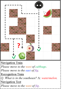
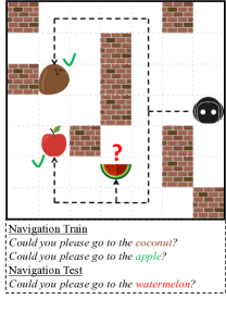
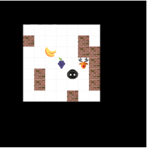
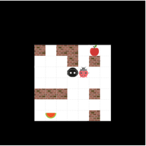
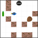
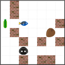
This paper describes a framework that demonstrates the zero-shot learning ability of an agent in a specific task, namely, learning to navigate in a 2D maze-like environment called xworld (Figure 1). We are interested in solving a similar task that is faced by a baby who is learning to walk and navigate, at the stage of learning his parents’ language. The parents might give some simple navigation command consisting of only two or three words in the beginning, and gradually increase the complexity of the command as time goes by. Meanwhile, the parents might teach the baby the language in some other task such as object recognition. After the baby understands the language and masters the navigation skill, he could immediately navigate to a new concept that is learned from object recognition but never appeared in the navigation command before.
We train our baby agent across many learning sessions in xworld. In each session, the agent perceives the environment through a sequence of raw-pixel images, a natural language command issued by a teacher, and a set of rewards. The agent also occasionally receives the teacher’s questions on object recognition whenever certain conditions are triggered. By exploring the environment, the agent learns simultaneously the visual representations of the environment, the syntax and semantics of the language, and how to navigate itself in the environment. The whole framework employed by the agent is trained end to end from scratch by gradient descent. We test the agent under four different command conditions, three of which require that the agent generalizes to interpret unseen commands and words, and that the framework architecture is modular so that other modules such as perception and action will still work properly under such circumstance. Our experiments show that the agent performs equally well ( average success rate) in all conditions. Moreover, several baselines that simply learn a joint embedding for image and language yield poor results.
In summary, our main contributions are two-fold:
-
A new deep reinforcement learning (DRL) task that integrates both vision and language. The language is not pre-parsed (Sukhbaatar et al., 2016) or -linked (Mikolov et al., 2015; Sukhbaatar et al., 2016) to the environment. Instead, the agent has to learn everything from scratch and ground the language in vision. This task models a similar scenario faced by a learning child.
-
The zero-shot learning ability by leveraging the compositionality of both the language and the network architecture. We believe that this ability is a crucial component of human-level intelligence.
2 Related Work
Our work is inspired by the research of multiple disciplines. Our xworld is similar to the MazeBase environment (Sukhbaatar et al., 2016) in that both are 2D rectangular grid world. One big difference is that their quasi-natural language is already parsed and linked to the environment. They put more focus on reasoning and planning but not language acquisition. On the contrary, we emphasize on how to ground the language in vision and generalize the ability of interpreting the language. There are several challenging 3D environments for RL such as ViZDoom (Kempka et al., 2016) and DeepMind Lab (Beattie et al., 2016). The visual perception problems posed by them are much more difficult than ours. However, these environments do not require language understanding. Our agent needs to learn to interpret different goals from different natural language commands.
Our setting of language learning shares some similar ideas of the AI roadmap proposed by Mikolov et al. (2015). Like theirs, we also have a teacher in the environment that assigns tasks and rewards to the agent. The teacher also provides additional questions and answers to the agent in an object recognition task. Unlike their proposal of entirely using linguistic channels, our tasks involve multiple modalities and are more similar to human experience.
The importance of compositionality and modularity of a learning framework has been discussed at length in cognitive science by Lake et al. (2016). The compositionality of our framework is inspired by the ideas in Neural Programmer (Neelakantan et al., 2016) and Neural Module Networks (NMNs)(Andreas et al., 2016a, b). Neural Programmer is trained with backpropagation by employing soft operations on databases. NMNs assemble several primitive modules according to questions in Visual Question Answering (VQA). It depends on an external parser to convert each sentence to one or several candidate parse trees and thus cannot be trained end to end. We adapt their primitive modules to our framework with differentiable computation units to enable gradient calculation. Their subsequent work (N2NMNs) (Hu et al., 2017) learns end to end to optimize over the full space of parse trees, but relies on candidate parse trees as an expert policy used by a behavior cloning procedure to initialize the policy parameters.
Our recognition task is essentially image VQA (Antol et al., 2015; Gao et al., 2015; Ren et al., 2015; Lu et al., 2016; Andreas et al., 2016a, b; Teney and Hengel, 2016; Yang et al., 2016). The navigation task can also be viewed as a VQA problem if the actions are treated as answer labels. Moreover, it is a zero-shot VQA problem (i.e., test questions containing unseen concepts) which has not been well addressed yet.
Our language acquisition problem is closely related to some recent work on grounding language in images and videos (Yu and Siskind, 2013; Rohrbach et al., 2016; Gao et al., 2016). The navigation task is also relevant to robotics navigation under natural language command (Chen and Mooney, 2011; Tellex et al., 2011; Barrett et al., 2015). However, they either assume annotated navigation paths in the training data or do not ground language in vision. As xworld is a virtual environment, we currently do not address mechanics problems encountered by a physical robot, but focus on its mental model building.
3 xworld Environment
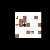
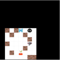
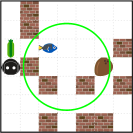
We first briefly describe the xworld environment. More details are in Appendix 8.5. xworld is a 2D grid world (Figure 1). An agent interacts with the environment over a number of time steps , with four actions: up, down, left, and right. It does so for many sessions. At the beginning of each session, a teacher starts a timer and issues a natural language command asking the agent to reach a location referred to by objects in the environment. There might be other objects as distractors. Thus the agent needs to differentiate and navigate to the right location. It perceives the entire environment through RGB pixels with an egocentric view (Figure 2c). If the agent correctly executes the command before running out of time, it gets a positive reward. Whenever it hits a wall or steps on an object that is not the target, it gets a negative reward. The agent also receives a small negative reward at every step as a punishment for taking too much time. After each session, the environment is reset randomly.
Some example commands are (the parentheses contain environment configurations that are withheld from the agent, same below):
-
Please navigate to the apple. (There is an apple, a banana, an orange, and a grape.)
-
Can you move to the grid between the apple and the banana? (There is an apple and a banana. The apple and the banana are separated by one empty grid.)
-
Could you please go to the red apple? (There is a green apple, a red apple, and a red cherry.)
The difficulty of this navigation task is that, at the very beginning the agent knows nothing about the language: every word appears equally meaningless. After trials and errors, it has to figure out the language syntax and semantics in order to correctly execute the command.
While the agent is exploring the environment, the teacher also asks object-related questions whenever certain conditions are triggered (all conditions are listed in Appendix 8.5). The answers are always single words and provided by the teacher for supervision. Some example QA pairs are:
-
Q:What is the object in the north? A:Banana. (The agent is by the south of a banana, by the north of an apple, and by the west of a cucumber.)
-
Q:Where is the banana? A:North. (The agent is by the south of a banana and the east of an apple.)
-
Q:What is the color of the object in the west of the apple? A:Yellow. (An apple has a banana on its west and a cucumber on its east.)
We expect the agent to transfer the knowledge exclusively learned from this recognition task to the navigation task to execute zero-shot commands. Both the commands and questions are generated from templates (Appendix 8.5) and are made like human-elicited sentences.
 |
 |
4 Compositional Framework for Zero-shot Navigation
The zero-shot navigation problem can be formulated as training a policy with a grounding model:
that works correctly for a new test command which never appears in the training set. In the above formulation, is the agent’s navigation action, is the perceived environment, is the navigation goal attention computed by grounding the teacher’s command in the environment . Note that the policy depends on but not directly on , thus our key problem is essentially how to ground a new command to get the correct attention map.
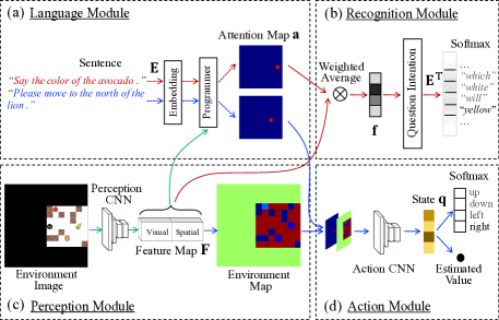
The proposed framework for solving this problem contains four major modules: perception (Section 4.1), recognition (Section 4.2), language (Section 4.3), and action (Section 4.4). The design of the framework is driven by the need of navigating under new command . Thus we will focus on how language grounding (Figure 2a) and recognition (Figure 2b) are related, and how to transfer the knowledge learned in the latter to the former. For an effective knowledge transfer, we believe that the framework has to possess three crucial properties:
-
PI
Language grounding and recognition have to be reduced to (approximately) the same problem. This ensures that a new word exclusively learned from recognition has already been grounded for attention.
-
PII
The language module must be compositional. It must process a sentence while preserving the (major) sentence structure. One example would be a parser that outputs a parse tree.
-
PIII
Inductive bias (Lake et al., 2016) must be learned from training sentences. The language module must know how to parse a sentence that has a previously seen structure even if a word position of the sentence is filled with a completely new word.
There is no existing framework for image captioning or VQA exhibits all such properties. While in theory, binding parameters or embeddings between the language module and the recognition module might satisfy the first property, in practice a naive binding without further architecture support hardly works. It is also challenging for a simple (gated) Recurrent Neural Network (RNN) to satisfy the last two properties when a sentence has a rich structure. Our framework detailed below is designed exactly for these three properties.
4.1 Generating Feature Map
We compute a feature map as an abstraction of the environment and the agent’s ego-centric geometry, on which we perform the recognition and grounding of the entire dictionary. Because of this general computation purpose, the map should not only encode visual information, but also provide spatial features. The feature map is formed by stacking two feature maps and along the channel dimension. The perception module (Figure 2c) transforms an environment image into the visual feature map through a Convolutional Neural Network (CNN), whose output has a spatial dimension equal to the number of grids in the environment, where each pixel corresponds to a grid. The spatial feature map is a set of randomly initialized parameters. Intuitively, is responsible for the agent’s visual sense while is responsible for its direction sense. The agent needs to learn to associate visually-related words with while associate spatially-related words with .
4.2 Recognizing and Grounding a Single Word
To achieve zero-shot navigation, we start with reducing the single-word recognition and grounding to the same problem, after which we will extend the reduction to the grounding of a sentence of multiple words (Section 4.3). The single-word grounding problem is defined as
| (1) |
where is a feature map, is the word index, is a spatial attention map, and is the number of pixels. Imagine that the feature map is a collection of slots of features, given a word , we need to find the corresponding slots (highlighted by attention) that match the word semantics. In a reverse way, the recognition problem is defined as
The recognition module (Figure 2b) outputs the most possible word for a feature map weighted by attention. This reflects the question answering process after the agent attending to a region of the environment image according to a question. In the extreme case, when is a one-hot vector, the module extracts and classifies one slot of feature. Suppose that the extracted feature is directly fed to a Softmax layer , where denotes the Softmax function over classes and is the parameter vector of the th class. Notice that the multiplication essentially treats as a filter and convolves it with every feature on . This computation operates as if it is solving the grounding problem in Eq. 1, and it produces an attention map which is optimized towards the following property
where is the groundtruth class for . In other words, this property implies that is grounded in where the feature of class locates. This is exactly where we need to ground word with embedding . Thus we set the Softmax matrix as the transpose of the word embedding table (i.e., ). So far, we have satisfied property PI for the single-word grounding case, namely, if a new word is trained to be recognized accurately, then it can also be grounded correctly without being trained to be grounded before.
There is still one flaw in the above definition of recognition. An attention map only tells the agent where, but not what, to focus on. Imagine a scenario in which the agent stands to the east of a red apple. Given an attention map that highlights the agent’s west, should the agent answer west, apple, or red? It turns out that the answer should also depend on the question itself, i.e., the question intention has to be understood. Therefore, we redefine the recognition problem as:
where is the question and computes its intention. In our framework, is modeled as a gated RNN (Cho et al., 2014) which outputs an embedding mask through Sigmoid. Then the Softmax distribution becomes (Figure 2b), where denotes element-wise multiplication. To make property PI still possible, we modify the grounding problem so that a word embedding is masked before it is grounded:
| (2) |
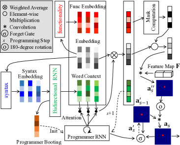
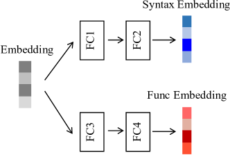
where is modeled as a projection111We use “projection” to denote the process of going through one or more fully-connected (FC) layers. that outputs an embedding mask through Sigmoid. Intuitively, it enhances the grounding with the ability of selecting features that are relevant to the word being grounded, and this selection is only decided by the word itself. Both functions and serve as the agent’s decision makers on which features to focus on given particular language tokens. They operate on the same intermediate word representation referred to as functionality embedding that is a projection of the word embedding (Figure 4 Appendix 8.7). Functionality embedding is exclusively used for computing embedding masks. Details of mask computation are in Figure 5 Appendix 8.7.
4.3 Grounding a Sentence
Now we extend single-word grounding to sentence grounding while trying to preserve property PI. The high-level idea is that we can ground a sentence by grounding individual words of that sentence through several steps, one or more words per step at a time. The questions we will answer in this section are how to: 1) decide which words to ground at each step, 2) combine the grounding results of these steps to reflect the grounding of the sentence, and 3) make the whole process differentiable.
The core of our language module (Figure 2a) is a differentiable programmer (Figure 2 Right). We treat each sentence (either navigation command or recognition question) as a program command. The programmer converts the command implicitly to a set of operations (see Appendix 8.2 for an analogy between the operations of NMNs and ours). The programming result is an attention map. For navigation, the attended regions indicate the target locations. For recognition, they indicate which part of the environment to be recognized. The programmer programs a command in several steps. At each step, the programming consists of three substeps: attending, grounding, and combining. The programmer first softly attends to a portion of a sentence. Once one or more words are attended, they are extracted, modulated by the embedding mask, and grounded in image. The resulting attention map is selectively combined with the maps in the previous steps (detailed below). In this way, the programmer uses the dynamic word attention, the grounding process modulated by masks, and the selective map combination to implicitly output a network layout and model the structural process of grounding a sentence in image. This approximately satisfies property PII.
The word attention is determined by the global sentential context, the local context at each word, and the history of a programmer RNN. Both global and local contexts are computed based on an intermediate word representation referred to as syntax embedding that is a projection of the word embedding (Figure 4 Appendix 8.7). Intuitively, the syntax embedding can be trained to encode a group of words similarly if they have the same syntactic meaning. Thus when a sentence contains a new word that was only trained in recognition, the programmer RNN has the inductive bias of interpreting the sentence as if the new word is an existing word with the same syntactic meaning (property PIII). The details of word attention are in Appendix 8.1 and omitted here due to page limit.
With the word attention at each step , we compute the averaged word embedding, mask it given the corresponding averaged functionality embedding, and convolve it with the feature map as in the single-word case (Eq. 2). The convolution result is input to a Softmax layer to get a sum-to-one attention map . Assume that we cached an attention map in the previous step. The programmer approximates the 2D translation of spatial attention by , where denotes the 180-degree rotation. Then the programmer caches a new attention map through a forget gate: , where the gate is computed from the current state of the programmer RNN (Figure 2 Right). We set where is a map whose center pixel is one and the rest are all zeros. Finally, the attention map at the last step is used as the output of the programmer.
4.4 Navigation
A navigation attention map only defines the target locations. To navigate, the agent needs to know the surrounding environment including obstacles and distractors. Our perception module (Figure 2c) convolves with a filter to get the environment map. We stack the two maps and input them to an action CNN whose output is projected to a state vector that summarizes the environment. The state vector is further projected to a distribution over the actions. At each time step, the agent takes action with a probability of , where is the rate of random exploration. The state is also projected to a scalar to approximate value function.
5 Training
Our training objective contains two sub-objectives , one for navigation and the other for recognition, where are the joint parameters of the framework. Most parameters are shared between the two tasks222In all the figures of our framework, components with the same name share the same set of parameters.. We model the recognition loss as the multi-class cross entropy which has the gradients
where is the expectation over all the questions asked by the teacher in all training sessions, is the correct answer to each question, and is the corresponding feature. We compute the navigation loss as the negative expected reward the agent receives by following its policy . With the Actor-Critic (AC) algorithm (Sutton and Barto, 1998), we have the approximate gradients
where are the target parameters that are periodically (every minibatches) copied from , is the immediate reward, is the discount factor, is the next state after taking action at state , and and are the policy and value output by the action module. Since the expectations and are different, we optimize the two sub-objectives separately over the same number of minibatches. For effective training, we employ Curriculum Learning (Bengio et al., 2009) and Experience Replay (Mnih et al., 2015) with Prioritized Sampling (Schaul et al., 2016) (Appendix 8.6).
6 Experiments
We use Adagrad (Duchi et al., 2011) with a learning rate of for Stochastic Gradient Descent (SGD). In all experiments, we set the batch size to 16 and train 200k batches. The target parameters are updated every batches. The reward discount factor is set to . All the parameters have a default weight decay equal to batch size. For each layer, by default its parameters have zero mean and a standard deviation of , where is the number of parameters of that layer. The agent has 500k exploration steps in total, and the exploration rate decreases linearly from to . We fix the number of programming steps as 3, and train each model with 4 random initializations. The whole framework is implemented with PaddlePaddle (https://github.com/PaddlePaddle/Paddle/) and trained end to end. More implementation details are in Appendix 8.3.
Baselines We first compare with five baselines in a normal setting.
-
SimpleAttention We modify our framework by replacing the programmer with a simple attention model. Given a sentence, we use an RNN to output an embedding which is convolved as a filter with the visual feature map to get an attention map. The rest of our framework is unchanged (Figure 7 Appendix 8.7). This baseline is an ablation to show the necessity of the programmer.
-
NoTransShare We do not tie the word embedding table to the transposed Softmax matrix. In this case, language grounding and recognition are not the same problem. This baseline is an ablation to show the impact of the transposed sharing on the training convergence.
-
SAN We replace our language module with the attention process of Stacked Attention Network (SAN) (Yang et al., 2016), with the difference of training a CNN from scratch, instead of using a pretrained one, to accommodate to xworld. The rest of our framework is unchanged.
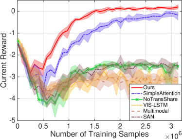 |
For each method, we test 10k sessions in total over four navigation subtasks nav_obj, nav_col_obj, nav_nr_obj, and nav_bw_obj (Appendix 8.5). We compute the success rates where success means that the agent reaches the target location in time in a test session. The training reward curves and the success rates are shown in Figure 3 and Table 1a, respectively. VIS-LSTM and Multimodal have poor results because they do not ground language in vision. SAN has the same overall architecture with our framework but with a different language module, which requires it to generate accurate navigation attention map because the navigation action solely depends on attention maps rather than visual image features as in VIS-LSTM and Multimodal. This assumption is a quite strong one and our experiment result shows that even though SAN gets 100% recognition accuracy, its action module hardly works. Our explanation is that SAN reasons spatial relationships based on the encoding of multiple neighboring objects in a single feature at each convolution location (i.e., a broad receptive field), which can easily lead to attention diffusion. Its recognition module might be able to still correctly classify given diffused attention, but the action module requires far more accurate attention as the navigation signal for the agent. Surprisingly, NoTransShare converges much slower than our framework does. One possible reason is that the correct behavior of the language module is hard to be found by SGD if no constraint on word embedding is imposed. Although SimpleAttention is able to perform well, without word-level attention, its ability of sentence understanding is limited.
Zero-shot Navigation Our primary question is whether the agent has the zero-shot navigation ability of executing previously unseen commands. We setup four command conditions for training the agent:
-
Standard The training command set has the same distribution with the test command set.
-
NC Some word combinations are excluded from the training command set, even though all the words are in it. We specifically consider three types of word combinations: (object, location), (object, color), and (object, object). We enumerate all combinations for each type and randomly hold out 10% from the teacher in navigation.
-
NWNav&NWNavRec Some object words are excluded from navigation training, and are trained only in recognition and tested in navigation as new concepts. NWNavRec guarantees that the new words will not appear in questions but only in answers while NWNav does not. We randomly hold out 10% of the object words.
|
|||||||||||||||||||||||||||||||||||||||||||||
| (a) | |||||||||||||||||||||||||||||||||||||||||||||
|
|||||||||||||||||||||||||||||||||||||||||||||
| (b) |
We use SimpleAttention for comparison as the other baselines have far worse performance than it in the previous experiment. Both SimpleAttention and our framework are trained under each condition without changing the their hyperparameters. For testing, we put the held-out combinations/words back to the commands (i.e., Standard condition) and again test 10k sessions. Table 1b contains the success rates. Our framework gets almost the same success rates for all the conditions, and obtains high zero-shot success rates. The results of NWNavRec show that although some new object concepts are learned from a completely different problem, they can be tested on navigation without any model retraining or finetuning. In contrast, SimpleAttention almost fails on zero-shot commands (especially on NWNavRec). Interestingly, in nav_bw_obj it has a much higher zero-shot success rate than in the other subtasks. Our analysis reveals that with the filter, it always highlights the location between two objects without detecting their classes, because usually there is only one qualified pair of objects in the environment for nav_bw_obj. As a result, it does not really generalize to unseen commands.
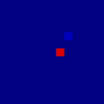
Visualization and Analysis Our framework produces intermediate results that can be easily visualized and analyzed. One example has been shown in Figure 2, where the environment map is produced by a trained perception module. It detects exactly all the obstacles and goals. The map constitutes the learned prior knowledge for navigation: all walls and goals should be avoided by default because they incur negative rewards. This prior, combined with the attention map produced for a command, contains all information the agent needs to navigate. The attention maps are usually very precise (Figure 10 Appendix 8.7), with some rare cases in which there are flaws, e.g., when the agent needs to navigate between two objects. This is due to our simplified assumption on 2D geometric translation: the attention map of a location word is treated as a filter and the translation is modeled as convolution. This results in attention diffusion in the above case. To address this issue, more complicated transformation can be used (e.g., FC layers).
We also visualize the programming process. We observe that the programmer RNN is able to shift its focus across steps (Figure 11 Appendix 8.7). With additional analysis of the grounding and map operations, we find that in the first example, the programmer essentially does Transform[southeast](Find[cabbage]()), and in the second example, it essentially performs Transform[between](CombineOr(Find[apple](), Find[coconut]())).
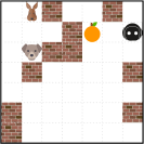
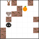
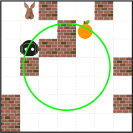
We find the attention and environment maps very reliable by visualization. This is verified by the 100% QA accuracy in recognition. However, in Table 1 the best success rate is still away from the perfect. Further analysis reveals that the agent tends to stuck in loop if the target location is behind a long wall, although it has a certain chance to bypass it (Figure 12 Appendix 8.7). Thus we believe that the discrepancy between the good map quality and the imperfect performance results from our action module. Currently the action module learns a direct mapping from an environment state to an action. There is no support for either history remembering or route planning (Tamar et al., 2016). Since our focus here is zero-shot navigation, we leave such improvements to future work.
7 Conclusion
We have demonstrated an end-to-end compositional framework for a virtual agent to generalize an existing skill to new concepts without being retrained. Such generalization is made possible by reusing knowledge, encoded by language and learned in other tasks. By assembling words in different ways, the agent is able to tackle new tasks while exploiting existing knowledge. We reflect these ideas in the design of our framework and apply it to a concrete example: zero-shot navigation in xworld. Our framework is just one possible implementation. Our claim is not that an intelligent agent must have a mental model as the presented one, but it has to possess several crucial properties discussed in Section 4. Currently the agent explores in a 2D environment. In the future, we plan to migrate the agent to a 3D world like Malmo (Johnson et al., 2016). There will be several new challenges, e.g., perception and geometric transformation will be more difficult to model. We hope that the current framework provides some preliminary insights on training a similar agent in a 3D environment.
Acknowledgments
We thank Yuanpeng Li, Liang Zhao, Yi Yang, Zihang Dai, Qing Sun, Jianyu Wang, and Xiaochen Lian for their helpful suggestions on writing.
References
- Andreas et al. [2016a] J. Andreas, M. Rohrbach, T. Darrell, and D. Klein. Neural module networks. In CVPR, pages 39–48, 2016a.
- Andreas et al. [2016b] J. Andreas, M. Rohrbach, T. Darrell, and D. Klein. Learning to compose neural networks for question answering. In ACL, pages 1545–1554, 2016b.
- Antol et al. [2015] S. Antol, A. Agrawal, J. Lu, M. Mitchell, D. Batra, C. Lawrence Zitnick, and D. Parikh. Vqa: Visual question answering. In ICCV, pages 2425–2433, 2015.
- Barrett et al. [2015] D. P. Barrett, S. A. Bronikowski, H. Yu, and J. M. Siskind. Robot language learning, generation, and comprehension. arXiv preprint arXiv:1508.06161, 2015.
- Beattie et al. [2016] C. Beattie, J. Z. Leibo, D. Teplyashin, T. Ward, M. Wainwright, H. Küttler, A. Lefrancq, S. Green, V. Valdés, A. Sadik, J. Schrittwieser, K. Anderson, S. York, M. Cant, A. Cain, A. Bolton, S. Gaffney, H. King, D. Hassabis, S. Legg, and S. Petersen. Deepmind lab. CoRR, abs/1612.03801, 2016.
- Bengio et al. [2009] Y. Bengio, J. Louradour, R. Collobert, and J. Weston. Curriculum learning. In ICML, pages 41–48, 2009.
- Chen and Mooney [2011] D. L. Chen and R. J. Mooney. Learning to interpret natural language navigation instructions from observations. In AAAI, volume 2, pages 1–2, 2011.
- Cho et al. [2014] K. Cho, B. van Merrienboer, Ç. Gülçehre, F. Bougares, H. Schwenk, and Y. Bengio. Learning phrase representations using RNN encoder-decoder for statistical machine translation. In EMNLP, 2014.
- Duchi et al. [2011] J. Duchi, E. Hazan, and Y. Singer. Adaptive subgradient methods for online learning and stochastic optimization. JMLR, 12(Jul):2121–2159, 2011.
- Gao et al. [2015] H. Gao, J. Mao, J. Zhou, Z. Huang, L. Wang, and W. Xu. Are you talking to a machine? dataset and methods for multilingual image question. In NIPS, pages 2296–2304, 2015.
- Gao et al. [2016] Q. Gao, M. Doering, S. Yang, and J. Y. Chai. Physical causality of action verbs in grounded language understanding. In ACL, volume 1, pages 1814–1824, 2016.
- Hu et al. [2017] R. Hu, J. Andreas, M. Rohrbach, T. Darrell, and K. Saenko. Learning to reason: End-to-end module networks for visual question answering. arXiv preprint arXiv:1704.05526, 2017.
- Johnson et al. [2016] M. Johnson, K. Hofmann, T. Hutton, and D. Bignell. The malmo platform for artificial intelligence experimentation. In IJCAI, 2016.
- Kempka et al. [2016] M. Kempka, M. Wydmuch, G. Runc, J. Toczek, and W. Jaśkowski. ViZDoom: A Doom-based AI research platform for visual reinforcement learning. In IEEE Conference on Computational Intelligence and Games, pages 341–348, 2016.
- Kiela et al. [2016] D. Kiela, L. Bulat, A. L. Vero, and S. Clark. Virtual embodiment: A scalable long-term strategy for artificial intelligence research. In NIPS Workshop, 2016.
- Lake et al. [2016] B. M. Lake, T. D. Ullman, J. B. Tenenbaum, and S. J. Gershman. Building machines that learn and think like people. Behavioral and Brain Sciences, pages 1–101, 11 2016.
- Lu et al. [2016] J. Lu, J. Yang, D. Batra, and D. Parikh. Hierarchical question-image co-attention for visual question answering. In NIPS, pages 289–297, 2016.
- Mao et al. [2015] J. Mao, X. Wei, Y. Yang, J. Wang, Z. Huang, and A. L. Yuille. Learning like a child: Fast novel visual concept learning from sentence descriptions of images. In ICCV, pages 2533–2541, 2015.
- Mikolov et al. [2015] T. Mikolov, A. Joulin, and M. Baroni. A roadmap towards machine intelligence. arXiv preprint arXiv:1511.08130, 2015.
- Mnih et al. [2015] V. Mnih, K. Kavukcuoglu, D. Silver, A. A. Rusu, J. Veness, M. G. Bellemare, A. Graves, M. Riedmiller, A. K. Fidjeland, G. Ostrovski, et al. Human-level control through deep reinforcement learning. Nature, 518(7540):529–533, 2015.
- Neelakantan et al. [2016] A. Neelakantan, Q. V. Le, and I. Sutskever. Neural programmer: Inducing latent programs with gradient descent. In ICLR, 2016.
- Ren et al. [2015] M. Ren, R. Kiros, and R. Zemel. Exploring models and data for image question answering. In NIPS, pages 2953–2961, 2015.
- Rohrbach et al. [2016] A. Rohrbach, M. Rohrbach, R. Hu, T. Darrell, and B. Schiele. Grounding of textual phrases in images by reconstruction. In ECCV, pages 817–834, 2016.
- Schaul et al. [2016] T. Schaul, J. Quan, I. Antonoglou, and D. Silver. Prioritized experience replay. In ICLR, 2016.
- Schuster and Paliwal [1997] M. Schuster and K. K. Paliwal. Bidirectional recurrent neural networks. IEEE Transactions on Signal Processing, 45(11):2673–2681, 1997.
- Sukhbaatar et al. [2016] S. Sukhbaatar, A. Szlam, G. Synnaeve, S. Chintala, and R. Fergus. Mazebase: A sandbox for learning from games. arXiv preprint arXiv:1511.07401, 2016.
- Sutton and Barto [1998] R. S. Sutton and A. G. Barto. Reinforcement learning: An introduction, volume 1. MIT press Cambridge, 1998.
- Tamar et al. [2016] A. Tamar, S. Levine, P. Abbeel, Y. WU, and G. Thomas. Value iteration networks. In NIPS, pages 2146–2154, 2016.
- Tellex et al. [2011] S. Tellex, T. Kollar, S. Dickerson, M. R. Walter, A. G. Banerjee, S. Teller, and N. Roy. Understanding natural language commands for robotic navigation and mobile manipulation. In AAAI, 2011.
- Teney and Hengel [2016] D. Teney and A. v. d. Hengel. Zero-shot visual question answering. arXiv preprint arXiv:1611.05546, 2016.
- Yang et al. [2016] Z. Yang, X. He, J. Gao, L. Deng, and A. Smola. Stacked attention networks for image question answering. In CVPR, pages 21–29, 2016.
- Yu and Siskind [2013] H. Yu and J. M. Siskind. Grounded language learning from video described with sentences. In ACL, pages 53–63, 2013.
8 Appendix
8.1 Word Attention
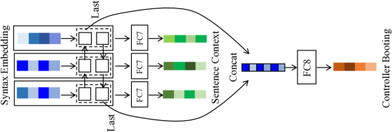
A sentence of length is first converted to a sequence of word embeddings by looking up the embedding table . Then the embeddings are projected to syntax embeddings (Figure 4). The syntax embeddings are fed into a Bidirectional RNN (Schuster and Paliwal, 1997) to obtain word context vectors . The last forward state and the first backward state are concatenated and projected to a booting vector (Figure 6), which is used to initialize the programmer RNN. Given a fixed number of programming steps, at each step the programmer RNN computes the attention for each word from its context vector :
where and are projection parameters, is the RNN state, is the activation function, and is the Softmax function over words. Then the context vectors are weighted averaged by the attention and fed back to the RNN to tell it how to update its hidden state.
8.2 Programmer Operations
The embedding masks produced by and support switching among the DescribeColor, DescribeLocation, and DescribeName operations by masking word embeddings according to given language tokens (Section 4.2). The selective map combination in Figure 2 Right supports nine different TranslateAttention operations by convolution. Our soft word attention supports the CombineAnd and CombineOr operations by attending to multiple words simultaneously. For example, when multiple objects are attended, the resulting attention map would be a union of the maps of the individual objects. When an object and the color modifying that object are both attended, the resulting attention map would be an intersection of the two maps, thus selecting the object with the correct color from a set of objects with the same name. Thus compared to NMNs (Andreas et al., 2016a), we end up with an implementation of an implicit and differentiable modular network.
8.3 Implementation Details
The agent at each time step receives a RGB image. This image is egocentric and includes both the environment and the black padding region. The agent processes the input image with a CNN that has four convolutional layers: , where represents filters with stride . All the four layers have the ReLU activation function. The output is the visual feature map with channels. We stack it along the channel dimension with another parametric spatial feature map of the same sizes. This spatial feature map is initialized with zero mean and standard deviation (Figure 2c).
The agent also receives a navigation command at the beginning of a session. The same command is repeated until the end of the session. The agent may or may not receive a question at every time step. The dimensions of the word embedding, syntax embedding, and functionality embedding are , , and , respectively. The word embedding table is initialized with zero mean and a standard deviation of 1. The hidden FC layers for computing the syntax and functionality embeddings have units (Figure 4). The bidirectional RNN for computing word contexts has a state size of in both directions. The output RNN booting vector and word context also have a length of . The state size of the programmer RNN is equal to the length of the booting vector (Figure 2 Right). The hidden FC layer for converting a functionality embedding to an embedding mask has a size of . The RNN used for summarizing the question intention has states (Figure 5). All FC layers and RNN states in the language and recognition module use Tanh as the activation function. The only exception is the FC layer that outputs the embedding mask (Sigmoid).
In the action module, the action CNN for processing the attention map and the environment map has two convolutional layers and , both with paddings of 1. They are followed by three FC layers that all have units. All five layers use the ReLU activation function.
8.4 Baseline Models
The language module of SimpleAttention has the word embedding size of . The RNN has the same size with the word embedding. The FC layer that produces the filter has an output size of which is 9 times the channel number of the visual feature map. The rest of the layer configuration is the same with our framework. VIS-LSTM has a CNN with four convolutional layers , , , and . This is followed by three FC layers with size . The word embedding and the RNN both have sizes of . The RNN output goes through three FC hidden layers of size either for recognition or navigation. Multimodal has the same layer size configuration with that of VIS-LSTM. SAN has a CNN with four convolutional layers , , , and , where the last layer makes each grid have a receptive field. Its word embedding size and RNN state size are both . Following Yang et al. (2016), we use two attention layers.
The outputs of all layers of the above baselines are ReLU activated except for those that are designed as linearly activated.
8.5 xworld Setup
We configure square environments with sizes ranging from 3 to 7. We fix the size of the environment image by padding walls for smaller environments. Different sessions may have different map sizes. In each session,
-
The number of time steps is four times the map size.
-
The number of objects on the map is from 1 to 3.
-
The number of wall grids on the map is from 0 to 10.
-
The positive reward when the agent reaches the correct location is set to . The negative rewards for hitting walls and for stepping on non-target objects are set to and , respectively. The time step penalty is set to .
The teacher has a vocabulary size of 104, including 2 punctuation marks. There are 9 locations, 4 colors, and 40 distinct object classes. Each object class has object instances on average. Every time the environment is reset, a number of object classes are randomly sampled and an object instance is randomly sampled for each class. There are in total 16 types of sentences the teacher can speak, including 4 types of navigation commands and 12 types of recognition questions. Each sentence type has multiple non-recursive natural-language templates, and corresponds to a subtask the agent must learn to perform. In total there are 256,832 distinct sentences with 92,442 for the navigation task and 164,390 for the recognition task. The sentence length ranges from 2 to 12.
The object, location, and color words of the teacher’s language are listed below. These are the content words with actual meanings that can be grounded in the environment. All the other words are treated as grammatical words whose embeddings are only for interpreting sentence structures. The differentiation between content and grammatical words is automatically learned by the agent based on the teacher’s language and the environment. All words have the same form of representation.
| Object | Location | Color | Other |
|---|---|---|---|
| apple, avocado, banana, blueberry, butterfly, | east, west, | green, | ?, ., and, block, by, can, color, could, |
| cabbage, cat, cherry, circle, coconut, | north, south, | red, | destination, direction, does, find, go, |
| cucumber, deer, dog, elephant, fig, | northeast, northwest, | blue, | goal, grid, have, identify, in, is, locate, |
| fish, frog, grape, hedgehog, ladybug, | southeast, southwest, | yellow | located, location, me, move, name, |
| lemon, lion, monkey, octopus, orange, | between | navigate, near, nothing, object, of, on, | |
| owl, panda, penguin, pineapple, pumpkin, | one, OOV, please, property, reach, say, | ||
| rabbit, snake, square, squirrel, star, | side, target, tell, the, thing, three, to, | ||
| strawberry, triangle, turkey, turtle, watermelon | two, what, where, which, will, you, your |
The sentence types that the teacher can speak are listed below. Each sentence type corresponds to a subtask. The triggering condition describes when the teacher says that type of sentences. Besides the conditions shown, an extra condition for navigation commands is that the target location must be reachable from the current agent location. An extra condition for color-related questions is that the object color must be one of the four defined colors, and objects with other colors will be ignored in these questions. If at a time step there are multiple conditions triggered, we randomly sample one sentence type for navigation and another for recognition. After the sentence type is sampled, we generate the command or question according to the corresponding sentence templates.
| Sentence Type | Example | Triggering Condition |
|---|---|---|
| (Subtask) | ||
| nav_obj | Please go to the apple. | [C0] Beginning of a session. & |
| [C1] The referred object has a unique | ||
| name. | ||
| nav_col_obj | Could you please move to the red apple? | [C0] & [C2] There are multiple objects |
| that either have the same name | ||
| but different colors, or have different | ||
| names but the same color. | ||
| nav_nr_obj | The north of the apple is your destination. | [C0] & [C1] |
| nav_bw_obj | Navigate to the grid between apple and | [C0] & [C3] Both referred objects have |
| banana please. | unique names and are separated by | |
| one grid. | ||
| rec_col2obj | What is the red object? | [C4] There is only one object that |
| has the referred color. | ||
| rec_obj2col | What is the color of the apple? | [C1] |
| rec_loc2obj | Please tell the name of the object in the south. | [C5] The agent is near the referred |
| object. | ||
| rec_obj2loc | What is the location of the apple? | [C1] & [C5] |
| rec_loc2col | What color does the object in the east have? | [C5] |
| rec_col2loc | Where is the red object located? | [C4] & [C5] |
| rec_loc_obj2obj | Identify the object which is in the east of the apple. | [C1] & [C6] The referred object is |
| near another object | ||
| rec_loc_obj2col | What is the color of the east to the apple? | [C1] & [C6] |
| rec_col_obj2loc | Where is the red apple? | [C2] & [C5] |
| rec_bw_obj2obj | What is the object between apple and banana? | [C7] Both referred objects have |
| unique names and are separated by | ||
| one object. | ||
| rec_bw_obj2loc | Where is the object between apple and banana? | [C7] & [C8] The agent is near the |
| object in the middle. | ||
| rec_bw_obj2col | What is the color of the object between apple | [C7] |
| and banana? |
8.6 Experience Replay and Curriculum Learning
We employ Experience Replay (Mnih et al., 2015) for training both the navigation and recognition tasks. The environment inputs, rewards, and the actions taken by the agent at the most recent 10k time steps are stored in a replay buffer. During training, every time two minibatches of the same number of experiences are sampled from the buffer, one for computing and the other for computing . For the former, only individual experiences are sampled. We uniformly sample experiences from a subset of the buffer which contains the teacher’s questions. For the latter, we need to sample transitions (i.e., pairs of experiences) so that TD error can be computed. We sample from the entire buffer using the Rank-based Sampler (Schaul et al., 2016) which has proven to increase the learning efficiency by prioritizing rare experiences in the buffer.
Because in the beginning the language is quite ambiguous, it is difficult for the agent to start learning with a complex environment setup. Thus we exploit Curriculum Learning (Bengio et al., 2009) to gradually increase the environment complexity. We gradually change the following things linearly in proportional to , where is the number of sessions so far and is the number of curriculum sessions:
-
The number of grids of the environment.
-
The number of objects in the environment.
-
The number of wall grids.
-
The number of possible object classes that can appear in the environment.
-
The length of a navigation command or a recognition question.
We find that this curriculum is crucial for efficient learning, because in the early phase the agent is able to quickly master the meanings of the location and color words given only small ambiguity. After this, these words are used to guide the optimization when more and more new sentence structures and objects are added. In the experiments, we set during training while do not use any curriculum during test (maximal difficulty).
8.7 Figures
 |
|
| (a) | (b) |


| Watermelon is the | Reach the grid between | Red ladybug is the | Can you go to the |
|---|---|---|---|
| destination. | grape and deer. | target. | south of the elephant? |
 |
 |
 |
 |
 |
 |
 |
 |

| Could you please go to the dog? | Please reach south of the cucumber. | ||||
|---|---|---|---|---|---|
 |
 |
 |
 |
 |
 |