Understanding the Lomb-Scargle Periodogram
Abstract
The Lomb-Scargle periodogram is a well-known algorithm for detecting and characterizing periodic signals in unevenly-sampled data. This paper presents a conceptual introduction to the Lomb-Scargle periodogram and important practical considerations for its use. Rather than a rigorous mathematical treatment, the goal of this paper is to build intuition about what assumptions are implicit in the use of the Lomb-Scargle periodogram and related estimators of periodicity, so as to motivate important practical considerations required in its proper application and interpretation.
1 Introduction
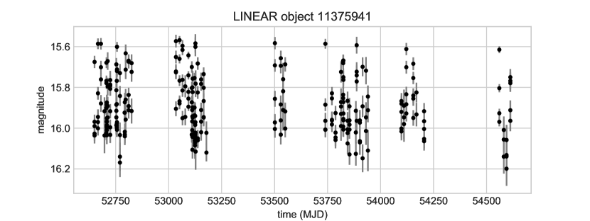
The Lomb-Scargle periodogram (Lomb, 1976; Scargle, 1982) is a well-known algorithm for detecting and characterizing periodicity in unevenly-sampled time-series, and has seen particularly wide use within the astronomy community. As an example of a typical application of this method, consider the data shown in LABEL:LINEAR-data: this is an irregularly-sampled timeseries showing a single object from the LINEAR survey (Sesar et al., 2011; Palaversa et al., 2013), with un-filtered magnitude measured 280 times over the course of five and a half years. By eye, it is clear that the brightness of the object varies in time with a range spanning approximately 0.8 magnitudes, but what is not immediately clear is that this variation is periodic in time. The Lomb-Scargle periodogram is a method that allows efficient computation of a Fourier-like power spectrum estimator from such unevenly-sampled data, resulting in an intuitive means of determining the period of oscillation.
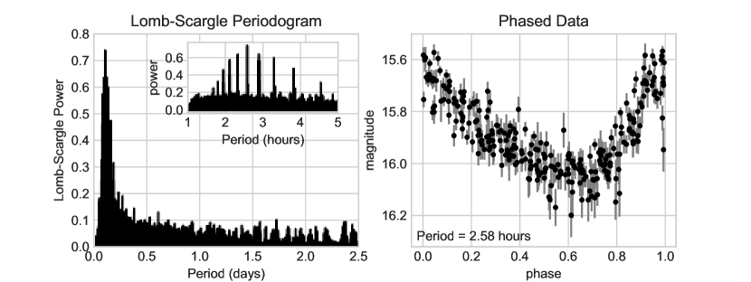
The Lomb-Scargle periodogram computed from this data is shown in the left panel of LABEL:LINEAR-power. The Lomb-Scargle periodogram here yields an estimate of the Fourier power as a function of period of oscillation, from which we can read-off the period of oscillation of approximately 2.58 hours. The right panel of LABEL:LINEAR-power shows a folded visualization of the same data as LABEL:LINEAR-data – i.e. plotted as a function of phase rather than time.
Often this is exactly how the Lomb-Scargle periodogram is presented: as a clean, well-defined procedure to generate a power spectrum and to detect the periodic component in an unevenly-sampled dataset. In practice, however, there are a number of subtle issues that must be considered when applying a Lomb-Scargle analysis to real-world datasets. Here are a few questions in particular that we might wish to ask about the results in LABEL:LINEAR-power:
-
1.
How does the Lomb-Scargle periodogram relate to the classical Fourier power spectrum?
-
2.
What is the source of the pattern of multiple peaks revealed by the Lomb-Scargle Periodogram?
-
3.
What is the largest frequency (i.e. Nyquist-like limit) that such an analysis is sensitive to?
-
4.
How should we choose the spacing of the frequency grid for our periodogram?
-
5.
What assumptions, if any, does the Lomb-Scargle approach make regarding the form of the unknown signal?
-
6.
How should we understand and report the uncertainty of the determined frequency?
Quantitative treatments of these sorts of questions are presented in various textbooks and review papers, but I have not come across any single concise reference that gives a good intuition for how to think about such questions. This paper seeks to fill that gap, and provide a practical, just-technical-enough guide to the effective use of the Lomb-Scargle method for detection and characterization of periodic signals. This paper does not seek a complete or rigorous treatment of the mathematics involved, but rather seeks to develop the intuition of how to think about these questions, with references to relevant technical treatments.
1.1 Why Lomb-Scargle?
Before we begin exploring the Lomb-Scargle periodogram in more depth, it is worth briefly considering the broader context of methods for detecting and characterizing periodicity in time series. First, it is important to note that there are many different modes of time series observation. Point observation like that shown in LABEL:LINEAR-data is typical of optical astronomy: values (often with uncertainties) are measured at discrete point in time, which may be equally or unequally-spaced. Other modes of observation—e.g., time-tag-events, binned event data, time-to-spill events, etc.—are common in high-energy astronomy and other areas. We will not consider such event-driven data modes here, but note that there have been some interesting explorations of unified statistical treatments of all of the above modes of observation (e.g. Scargle, 1998, 2002).
Even limiting our focus to point observations, there are a large number of complementary techniques for periodic analysis, which generally can be categorized into a few broad categories:
- Fourier Methods
-
are based on the Fourier transform, power spectra, and closely related correlation functions. These methods include the classical or Schuster periodogram (Schuster, 1898), the Lomb-Scargle periodogram (Lomb, 1976; Scargle, 1982), the correlation-based method of Edelson & Krolik (1988), and related approaches (see also Foster, 1996, for a discussion of wavelet transforms in this context).
- Phase-folding Methods
-
depend on folding observations as a function of phase, computing a cost function across the phased data (often within bins constructed across phase space) and optimizing this cost function across candidate frequencies. Some examples are String Length (Dworetsky, 1983), Analysis of Variance (Schwarzenberg-Czerny, 1989), Phase Dispersion Minimization (Stellingwerf, 1978), the Gregory-Laredo method (Gregory & Loredo, 1992), and the conditional entropy method (Graham et al., 2013a). Methods based on correntropy are similar in spirit, but do not always require explicit phase folding (Huijse et al., 2011, 2012).
- Least Squares Methods
-
involve fitting a model to the data at each candidate frequency, and selecting the frequency which maximizes the likelihood. The Lomb-Scargle periodogram also falls in this category (see Section 5), as does the Supersmoother approach (Reimann, 1994). Other studies recommend statistics other than least square residuals; see, e.g., the orthogonal polynomial fits of Schwarzenberg-Czerny (1996).
- Bayesian Approaches
-
apply Bayesian probability theory to the problem, often in a similar manner to the phase-folding and/or least-squares approaches. Examples are the generalized Lomb-Scargle models of Bretthorst (1988), the phase-binning model of Gregory & Loredo (1992), Gaussian process models (e.g. Wang et al., 2012), and models based on stochastic processes (e.g. Kelly et al., 2014).
Various reviews have been undertaken to compare the efficiency and effectiveness of the available methods; for example, Schwarzenberg-Czerny (1999) focuses on the statistical properties of methods and recommends those based on smooth model fits over methods based on phase binning, while Graham et al. (2013b) instead take an empirical approach and find that when considering detection efficiency in real datasets, no suitably efficient algorithm universally outperforms the others.
In light of this breadth of available methods, why limit our focus here to the Lomb-Scargle periodogram? One reason is cultural: the Lomb-Scargle periodogram is perhaps the best-known technique to compute periodicity of unequally-spaced data in astronomy and other fields, and so is the first tool many will reach for when searching for periodic content in a signal. But there is a deeper reason as well; it turns out that Lomb-Scargle occupies a unique niche: it is motivated by Fourier analysis (see Section 5), but it can also be viewed as a least squares method (see Section 6). It can be derived from the principles of Bayesian probability theory (see Section 6.5), and has been shown to be closely related to bin-based phase-folding techniques under some circumstances (see Swingler, 1989). Thus, the Lomb-Scargle periodogram occupies a unique point of correspondence between many classes of methods, and so provides a focus for discussion that has bearing on considerations involved in all of these methods.
1.2 Outline
The remainder of this paper is organized as follows:
Section 2 presents a review of the
continous Fourier transform and some of its useful properties,
including defining the notion of a power spectrum (i.e. classical/Schuster
periodogram) for detecting periodic content in a signal.
Section 3 builds on these properties to explore how
different observation patterns (i.e. window functions) affect the
periodogram, and discusses a conceptual understanding of the
Nyquist limiting frequency.
Section 4 considers non-uniformly sampled signals as
a special case of an observational window, and shows that the Nyquist-like
limit for this case is quite different than what many practitioners in
the field often assume.
Section 5 introduces the Lomb-Scargle periodogram,
a modified version of the classical periodogram for unevenly-sampled data,
as well as the motivation behind these modifications.
Section 6 discusses a complementary view of the
Lomb-Scargle periodogram as the result of least-squares model fitting,
as well as some extensions enabled by that viewpoint.
Section 7 builds on the concepts introduced
in earlier sections to discuss important practical considerations for
the use of the Lomb-Scargle periodogram, including the choice of
frequency grid, uncertainties and false alarm probabilities, and modes of
failure that should be accounted for when working with real-world data.
Section 8 concludes and summarizes the key recommendations
for practical use of the Lomb-Scargle periodogram.
2 Background: the Continuous Fourier Transform
In order to understand how we should interpret the Lomb-Scargle periodogram, we will first briefly step back and review the subject of Fourier analysis of continuous signals. Consider a continuous signal . Its Fourier transform is given by the following integral, where denotes the imaginary unit:
| (1) |
The inverse relationship is given by:
| (2) |
For convenience we will also define the Fourier transform operator , such that
| (3) | |||||
| (4) |
The functions and are known as a Fourier pair, which we will sometimes denote as .
2.1 Properties of the Fourier Transform
The continuous Fourier transform has a number of useful properties that we will make use of in our discussion.
- The Fourier transform is a linear operation.
-
That is, for any constant and any functions and , we can write:
(5) Both identities follow from the linearity of the Fourier integral.
- The Fourier transform of sinusoid with frequency is a sum of delta functions at .
-
From the integral definition of the Dirac delta function111 , we can write
(6) Using Euler’s formula222 for the complex exponential along with the linearity of the Fourier transform leads to the following identities:
(7) In other words, a sinusoidal signal with frequency has a Fourier transform consisting of a weighted sum of delta functions at .
- A time-shift imparts a phase in the Fourier transform.
-
Given a well-behaved function we can use a transformation of variables to derive the following identity:
(8) Notice that the time-shift does not change the amplitude of the resulting transform, but only the phase.
These properties taken together make the Fourier transform quite useful for the study of periodic signals. The linearity of the transform means that any signal made up of a sum of sinusoidal components will have a Fourier transform consisting of a sum of delta functions marking the frequencies of those sinusoids: that is, the Fourier transform directly measures periodic content in a continuous function.
Further, if we compute the squared amplitude of the resulting transform, we can both do away with complex components and remove the phase imparted by the choice of temporal baseline; this squared amplitude is usually known as the power spectral density or simply the power spectrum:
| (9) |
The power spectrum of a function is a positive real-valued function of the frequency that quantifies the contribution of each frequency to the total signal. Note that if is real-valued, it follows that is an even function; i.e. .
2.2 Some Useful Fourier Pairs
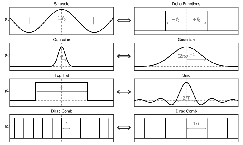
We have already discussed that the Fourier transform of a complex exponential is a single delta function. This is just one of many Fourier pairs to keep in mind as we progress to understanding the Lomb-Scargle periodogram. We list a few more important pairs here (see Figure 3 for a visual representation of the following pairs):
- The Fourier transform of a sinusoid is a pair of Delta functions.
-
(See
Figure 4: ) (10) We saw this above, but repeat it here for completeness.
- The Fourier transform of a Gaussian is a Gaussian.
-
(See
Figure 5: ) (11) The Gaussian function is given by
(12) - The Fourier transform of a rectangular function is a sinc function.
-
(See
Figure 6: ) (13) The rectangular function, , is a normalized symmetric function that is uniform within a range given by , and zero elsewhere:
(14) The sinc function is given by the standard definition:
(15) - The Fourier transform of a Dirac comb is a Dirac comb.
-
(See
Figure 7: ) (16) The Dirac comb, , is an infinite sequence of Dirac delta functions placed at even intervals of size :
(17)
Notice in each of these Fourier pairs the reciprocity of scales between a function and its Fourier transform: a narrow function will have a broad transform, and vice versa. More quantitatively, a function with a characteristic scale will in general have a Fourier transform with characteristic scale of . Such reciprocity is central to many diverse applications of Fourier analysis, from electrodynamics to music theory to quantum mechanics. For our purposes, this property will turn out to be quite important as we push further in understanding the Lomb-Scargle periodogram.
2.3 The Convolution Theorem
A final property of the Fourier transform that we will discuss here is its ability to convert convolutions into point-wise products. A convolution of two functions, usually denoted by the symbol, is defined as follows:
| (18) |
From the definition, it is clear that a convolution amounts to “sliding” one function past the other, integrating at each step. Such an operation is commonly used, for example, in smoothing a function, as visualized in Figure 8 for a rectangular smoothing window.
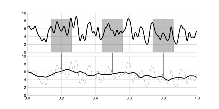
Given this definition of a convolution, it can be shown that the Fourier transform of a convolution is the point-wise product of the individual Fourier transforms:
| (19) |
In practice, this can be a much more efficient means of computing a convolution than to directly solve at each time the integral over that appears in Equation 18. The identity in Equation 19 is known as the convolution theorem, and is illustrated in LABEL:convolution-theorem.
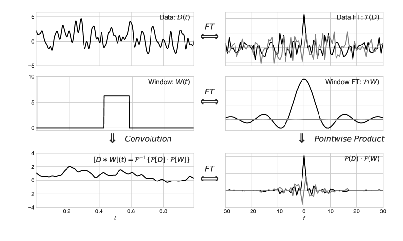
An important corrollary is that the Fourier transform of a product is a convolution of the two transforms:
| (20) |
We will see that these properties of the Fourier transform become essential when thinking about frequency components of time-domain measurements.
3 Window Functions: From Idealized to Real-world signals
Until now we have been discussing Fourier transforms of continuous signals which are well-defined for all times . Real-world temporal measurements of a signal, however, only involve some finite span of time, at some finite rate of sampling. In either case, the resulting data can be described by a point-wise product of the true underlying continuous signal with a window function describing the observation. For example, a continuous signal measured over a finite duration is described by a rectangular window function spanning the duration of the observation, and a signal measured at regular intervals is described by a Dirac comb window function marking those measurement times.
The Fourier transform of measured data in these cases, then, is not the transform of the continuous underlying function, but rather the transform of the point-wise product of the signal and the observing window. Symbolically, if the signal is and the window is , the observed function is
| (21) |
and by the convolution theorem, its transform is a convolution of the signal transform and the window transform:
| (22) |
This has some interesting consequences for the use and interpretation of periodograms, as we shell see.
3.1 Effect of a Rectangular Window
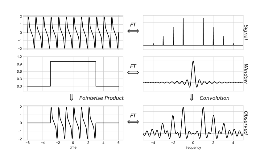
First, let’s consider the case of observing a continuous periodic signal over a limited span of time: LABEL:rectangular-window shows a continuous periodic function observed only within the window . The observed signal in this case can be understood as the pointwise product of the underlying infinite periodic signal with a rectangular window function. By the convolution theorem, the Fourier transform will be given by the convolution of the transform of the underlying function (here a set of delta functions at the component frequencies) and the transform of the window function (here a sinc function). For the purely periodic signal like the one seen in LABEL:rectangular-window, this convolution has the effect of replacing each delta function with a sinc function. Because of the inverse relationship between the width of the window and the width of its transform (see Figure 3), it follows that a wider observing window leads to proportionally less spread in the Fourier transform of the observed function.
3.2 The Dirac Comb and the Discrete Fourier Transform
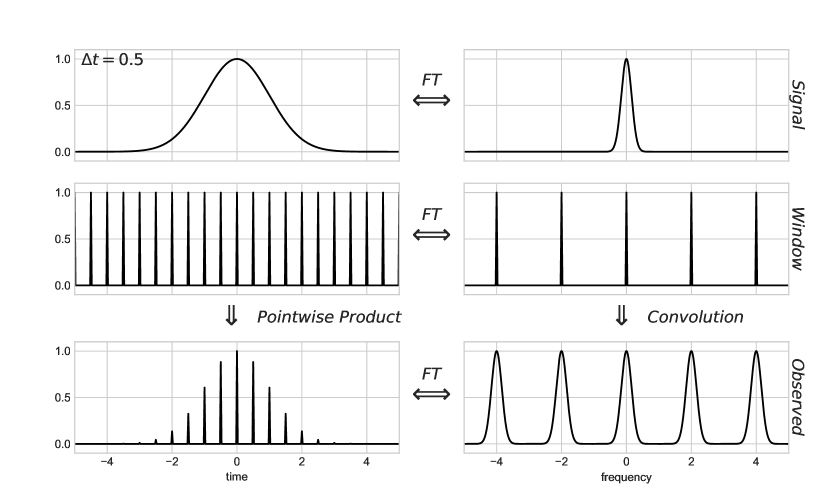
Another window function that commonly arises is when a continuous signal is sampled (nearly) instantaneously at regular intervals. Such an observation can be thought of as a point-wise product between the true underlying signal and a Dirac comb with the parameter matching the spacing of the observations; this is illustrated in LABEL:comb-window-1. Interestingly, because the Fourier transform of a Dirac comb is another Dirac comb, the effect of such an observing window is to create a long sequence of aliases of the underlying transform with a spacing of . With this in mind, we can be assured in this case that evaluating the observed transform in the range is sufficient to capture all the available frequency information: the signal outside that range is a sequence of identical aliases of what lies within that range.
3.2.1 The Nyquist Limit
The example in LABEL:comb-window-1 is somewhat of a best-case scenario, because the true Fourier transform values are non-zero only within a range of width . If we increase the time between observations, decreasing the spacing of the frequency comb, the true transform no longer “fits” inside the window transform, and we will have a situation similar to that in LABEL:comb-window-2. The result is a mixing of different portions of the signal, such that the true Fourier transform cannot be recovered from the transform of the observed data!
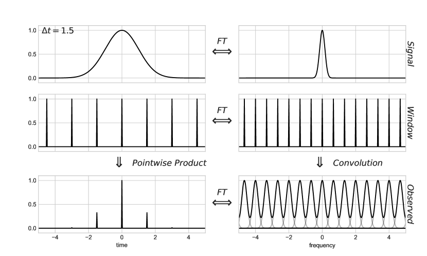
This implies that if we have a regularly-sampled function with a sampling rate of , we can only fully recover the frequency information if the signal is band-limited between frequencies . This is one way to motivate the famous Nyquist sampling limit, which approaches the question from the other direction and states that to fully represent the frequency content of a “band-limited signal” whose Fourier transform is zero outside the range , we must sample the data with a rate of at least .
3.2.2 The Discrete Fourier Transform
When a continuous function is sampled at regular intervals, the delta functions in the Dirac comb window serve to collapse the Fourier integral into a Fourier sum, and in this manner we can arrive at the common form of the discrete Fourier transform. Suppose we have a true (infinitely long and continuous) signal , but we observe it only at a regular grid with spacing . In this case, our observed signal is and its Fourier transform is
| (23) |
In the real world, however, we will not have an infinite number of observations, but rather a finite number of samples . We can choose the coordinate system appropriately and define to write
| (24) |
From the arguments around Nyquist aliasing, we know that the only relevant frequency range is from , and so we can define evenly-spaced frequencies with covering this range. Denoting the sampled transform as , we can write
| (25) |
which you might recognize as the standard form of the discrete Fourier transform.
Notice, though, that we glossed over one important thing: the effect of switching from an infinite number of samples to a finite number of samples. In moving from Equation 23 to Equation 24, we have effectively applied to our data a rectangular window function of width . From the discussion accompanying LABEL:rectangular-window, we know what this does: it gives us a Fourier transform convolved with a sinc function of width , resulting in the “smearing” of the Fourier transform signal with this width. Roughly speaking, then, any two Fourier transform values at frequencies within of each other will not be independent, and so we should space our evaluations of the frequency with . Comparing to above, we see that this is exactly the frequency spacing we arrived at from Nyquist-frequency arguments.
What this indicates is that the frequency spacing of the discrete Fourier transform is optimal in terms of both the Nyquist sampling limit and the effect of the finite observing window! Now, this argument has admittedly been a bit hand-wavy, but there do exist mathematically rigorous approaches to proving that the discrete Fourier transform in Equation 25 captures all of the available frequency information for a uniformly-sampled function (see, e.g. Vetterli et al., 2014). Despite our lack of rigor here, I find this to be a helpful approach in developing intuition regarding the relationship between the continuous and discrete Fourier transforms.
3.3 The Classical Periodogram
With the discrete Fourier transform defined in Equations 24-25, we can apply the definition of the Fourier power spectrum from Equation 9 to compute the classical periodogram, sometimes called the Schuster periodogram after Schuster (1898) who first proposed it:
| (26) |
Apart from the proportionality, this sum is precisely the Fourier power spectrum in Equation 9, computed for a continuous signal observed with uniform sampling defined by a Dirac comb. It follows that, in the uniform sampling case, the Schuster periodogram captures all of the relevant frequency information present in the data. This definition readily generalizes to the non-uniform case, which we will explore in the following section.
One point that should be emphasized is that the periodogram in Equation 26 and the power spectrum in Equation 9 are conceptually different things. As noted in Scargle (1982), the astronomy community tends to use these terms interchangeably, but to be precise the periodogram—i.e., the statistic we compute from our data—is an estimator of the power spectrum—i.e., the underlying continuous function of interest. In fact, the classical periodogram and its extensions (including the Lomb-Scargle we will discuss momentarily) are not consistent estimators of the power spectrum: that is, the periodogram has unavoidable intrinsic variance, even in the limit of an infinite number of observations (for a detailed discussion, see Chp 8.4 of Anderson, 1971).
4 Non-uniform Sampling
In the real world, particularly in fields like Astronomy where observations are subject to influences of weather and diurnal, lunar, or seasonal cycles, the sampling rate is generally far from uniform. Using the same approach as we used to explore uniform sampling in the previous section, we can now explore non-uniform sampling here.
In the general non-uniform case, we measure some signal at a set of times which we will denote , which leads to the following observing window:
| (27) |
Applying this window to our true underlying signal , we find an observed signal of the form:
| (28) | |||||
Just as in the evenly-sampled case, the Fourier transform of the observed signal is a convolution of the transforms of the true signal and the window:
| (29) |
Unlike in the uniform case, the window transform will generally not be a straightforward sequence of delta functions; the symmetry present in the Dirac comb is broken by the uneven sampling, leading the transform to be much more “noisy”. This can be seen in LABEL:random-window, which shows the Fourier transform of a non-uniform observing window with an average sampling rate identical to that in LABEL:comb-window-1, along with its imact on the observed Fourier transform.
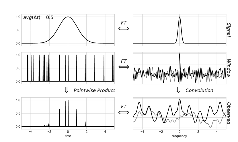
A few things stand-out in this figure. In particular, the Fourier transform of the non-uniformly spaced delta functions looks like random noise, and in some sense it is: the locations and heights of the Fourier peaks are related to the intervals between observations, and so randomization of observation times leads to a randomization of Fourier peak locations and heights. That is, non-structured spacing of observations will lead to a non-structured frequency peaks in the window transform. This non-structured window transform, when convolved with the Fourier transform of the true signal, results in an observed Fourier transform reflecting the same random noise. Comparing to the uniformly-spaced observations in LABEL:comb-window-1, we see that the unstructured nature of the window transform means that there is no exact aliasing of the true signal, and thus no way to exactly recover any portion of the true Fourier transform for the underlying function.
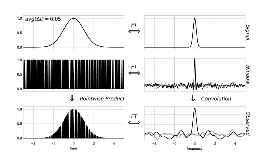
One might hope that sampling the signal more densely might alleviate these problems, and it does, but only to a degree. In Figure 14 we increase the density of observations by a factor of 10, such that there are 200 total observations over the length-10 observing window. The observed Fourier transform in this case is much more reflective of the underlying signal, but still contains a degree of “noise” rooted in the randomized frequency peaks due to randomized spacing between observations.
4.1 A Non-uniform Nyquist Limit?
We saw in Section 3.2.1 that the Nyquist limit is a direct consequence of the symmetry in the Dirac comb window function that describes evenly-sampled data, and uneven sampling destroys the symmetry that underlies its definition. Nevertheless, the idea of the “Nyquist frequency” seems to have taken hold in the scientific psyche to the extent that the idea is often mis-applied in areas where it is mathematically irrelevant. For unevenly-sampled data, the truth is that the “Nyquist limit” might or might not exist, and even in cases where it does exist it tends to be far larger (and thus far less relevant) than in the evenly-sampled case.
4.1.1 Incorrect Limits in the Literature
In the scientific literature it is quite common to come across various proposals for a Nyquist-like limit applied in the case of irregular sampling. A few typical approaches include using the mean of the sampling intervals (e.g. Scargle, 1982; Horne & Baliunas, 1986; Press et al., 2007), the harmonic mean of the sampling intervals (e.g. Debosscher et al., 2007), the median of the sampling intervals (e.g. Graham et al., 2013b), or the minimum sample spacing (e.g. Percy, 1986; Roberts et al., 1987; Press & Rybicki, 1989; Hilditch, 2001). All of these “pseudo-Nyquist” limits are tempting criteria in that they are easy to compute, and reduce to the classical Nyquist frequency in the limit of evenly-spaced data. Unfortunately, none of these approaches is correct: in general, unevenly-sampled data can probe frequencies far larger than any of these supposed limits (a fact that several of these citations do hint at parenthetically).
As a simple example of where such logic can fail spectacularly, consider the data from LABEL:LINEAR-data: though the mean sample spacing is one observation every seven days, in LABEL:LINEAR-power we were nevertheless able to quite clearly identify a period of 2.58 hours— an order of magnitude shorter than the average-based pseudo-Nyquist limit would indicate as possible. For the data in LABEL:LINEAR-data, the minimum sample spacing is just under 10 seconds, but it would be irresponsible to claim that this single pair of observations by itself defines some limit beyond which frequency information is unattainable.
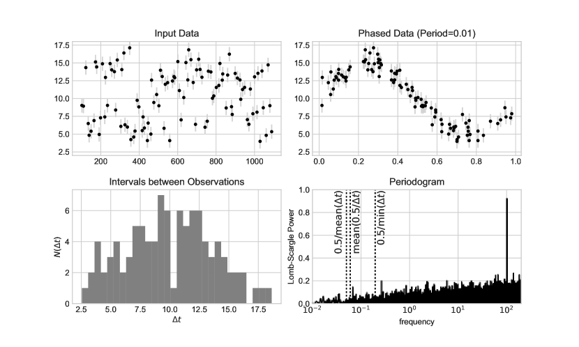
As a more extreme example, consider the data shown in LABEL:pseudo-nyquist. This consists of noisy samples from a sinusoid with a period of 0.01 units, with sample spacings ranging between 2 and 18 units: needless to say, any pseudo-Nyquist definition based on an average or minimum sample spacings will be far below the true frequency of 100; still, the the Lomb-Scargle periodogram in the lower right panel quite cleanly recovers the true frequency.
4.1.2 The Non-uniform Nyquist Limit
While pseudo-Nyquist arguments based on average or minimum sampling fail spectacularly, there is a sense in which the Nyquist limit can be applied to unevenly-spaced data. Eyer & Bartholdi (1999) explore this issue in some detail, and in particular prove the following:
Let be the largest value such that each can be written , for integers . The Nyquist Frequency then is .
In other words, computing the Nyquist limit for unevenly-spaced data requires finding the largest factor , such that each spacing is exactly an integer multiple of this factor. Eyer & Bartholdi (1999) prove this formally, but the result can be understood by thinking of such data as a windowed version of uniformly sampled data with spacing , where the window is zero at all points but the location of the observations. Such uniform data has a classical Nyquist limit of , and a window function applied on top of that sampling does not change that fact.
Figure 16 shows an example of such a Nyquist frequency. The data are non-uniformly sampled at times , with and drawn randomly from positive integers less than 10,000. According to the Eyer & Bartholdi (1999) definition, this results in a Nyquist frequency , and we see the expected behavior beyond this frequency: the signal at consists of a series of exact aliases of the signal at .
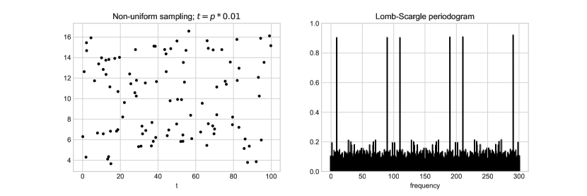
We should keep in mind one consequence of this Nyquist definition: if you have any pair of observation spacings whose ratio is irrational, the Nyquist limit does not exist!. To realize this situation in practice, however, would require infinitely precise measurements of the times ; finite precision of time measurements means the Nyquist frequency can be large, but not infinite. For example, if your observation times are recorded to decimal places, the Nyquist frequency will be at most
| (30) |
with the inequality due to the fact that larger common factors may exist. In other words, absent other relevant patterns in the observations, the Nyquist frequency for irregularly-sampled data is most typically set by the precision of the time measurements (see also Bretthorst, 2003; Koen, 2006, for more rigorous treatments of this result).
4.1.3 Frequency Limit due to Windowing
In contexts where observations are not instantaneous, but rather consist of short-duration integrations of a continuous signal, a qualitatively different kind of frequency limit exists. This is typical in, e.g., optical astronomy, where a single observation typically consists of an integration of observed photons over a finite duration . As noted by Ivezić et al. (2014), this time-scale of integration represents another kind of limiting frequency for irregularly-sampled data. Such a situation means that the observation is effectively a convolution of the underlying signal with a rectangular window function of width , in a manner analogous to LABEL:convolution-theorem. By the convolution theorem, the observed transform will be a point-wise product between the true transform and the transform of the window, which will generally have a width proportional to . This means that—absent other more constraining window effects—the frequency limit is , with the constant of proportionality dependent on the shape of the effective window describing individual observations.
Keep in mind that the windowing limit is quite different than a Nyquist limit: the Nyquist limit is the frequency beyond which all signal is aliased into the Nyquist range; the windowing limit is the frequency beyond which all signal is attenuated to zero. In practice, the limit implied by either the temporal resolution or windowing of individual observations may be too large to be computationally feasible; for discussion of frequency limits in practice, see Section 7.1.
4.2 Semi-structured Observing Windows
We have seen that for uniform data, the perfect aliasing beyond the Nyquist frequency is a direct consequence of the symmetry of the Dirac-comb window function. For non-uniform observations, such symmetry does not exist, but structure in the observing window can lead to partial aliasing of signals in the data (see, e.g. Deeming, 1975). In this section, we will examine two typical window functions derived from real-world observations: one ground-based (LINEAR) and one space-based (Kepler). For details on how window power spectra can be estimated in practice, see Section 7.3.
4.2.1 A Ground-based Observing Window: LINEAR
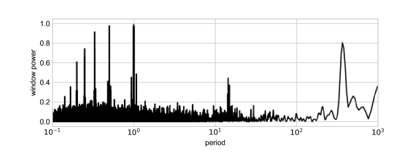
Let’s again consider the data shown in LABEL:LINEAR-data. The window power spectrum for this in LABEL:LINEAR-window shows some quite distinct features, and these features have an intuitive interpretation. Namely, if the window power shows a spike at a period of days, this means that an observation at time is likely to be followed by another observation near a time for integer .
With this in mind, the strong spike at a period of 1 day indicates that observations are taken near the same time of day: this is typical of a ground-based survey with observations recorded only during the nighttime hours. The additional spikes at periods of days (for integer ) are aliases of this same feature. LABEL:LINEAR-window also shows a wide spike at a period of 1 year, indicating a detectable annual pattern in the observations. Finally, there is a noticeable spike at approximately 14 days that is likely related to patterns of scheduling within the survey.
Recall that a Fourier spectrum observed through a particular window will reflect a convolution of the true spectrum and the window spectrum (cf. LABEL:random-window), and so we would expect the structure in the window to be imprinted on the power spectrum measured from the data.
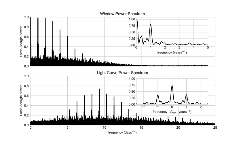
This imprint of the window power is illustrated in LABEL:LINEAR-window-effect. The upper panel shows the window power spectrum as a function of frequency (rather than period, as in LABEL:LINEAR-window), while lower panel shows the observed signal power spectrum as a function of frequency (rather than period, as in LABEL:LINEAR-power). The upper panel and its inset show clearly the 1-day and 1-year features we noted previously. The lower panel shows the observed power spectrum of the data: these diurnal and annual peaks in the window function are quite clearly imprinted on the observed power spectrum at relevant scales. This approximate aliasing is similar to the exact aliasing seen in regularly-sampled data at the Nyquist frequency; however, in this case the magnitude of the aliased signal fades further from the frequency driving the signal.
4.2.2 A Space-based Observing Window: Kepler
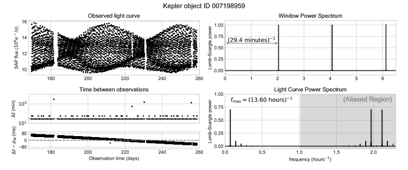
Space-based surveys will generally have quite different observing windows. For example, the upper-left panel of LABEL:kepler-data shows observations of an RR-Lyrae variable star from the Kepler survey, measured 4083 times over a period of three months, with an irregular observing cadence of around 30 minutes (For deeper discussion of these observations, see Kolenberg et al., 2010). The Kepler observations are very nearly uniformly-spaced, and this is reflected in the window power spectrum, shown in the upper-right panel of LABEL:kepler-data. The window function is a series of very narrow evenly-spaced spikes, reminiscent of the Dirac comb shown in Figures 11-12. By analogy we can treat minutes-1 as the effective Nyquist limit for the data, keeping in mind that aliasing beyond this “limit” will be imperfect due to the uneven spacing of the samples (see the lower-left panels of LABEL:kepler-data). The lower-right panel of LABEL:kepler-data shows the power spectrum of the observations, with gray shading indicating the (nearly) aliased region of the spectrum. The period of 13.6 hours is quite strongly apparent, along with smaller spikes at integer multiples of this frequency that indicate higher-order periodic components in the signal.
The window functions for ground-based and space-based observations, reflected by LINEAR data in LABEL:LINEAR-window-effect and Kepler data in LABEL:kepler-data, are quite different, but in both cases essential features of the observed power spectra can be understood by recognizing that the periodogram measures not the power spectrum of the underlying signal, but a power specrtrum from the convolution of the true signal transform and the Fourier transform of the window function.
5 From Classical to Lomb-Scargle Periodograms
Up until now, we have been mainly discussing the direct extension of the classical periodogram in Equation 26 to non-uniform data. Returning to this definition, we can rewrite the expression in a more suggestive way:
| (31) | |||||
Although this form of the non-uniform periodogram can be useful for identifying periodic signals, its statistical properties are not as straightforward as in the uniform case. When the classical periodogram is applied to uniformly-sampled Gaussian noise, the values of the resulting periodogram is chi-square distributed. This property becomes quite useful in practice when the periodogram is used in the context of a classical hypothesis test to distinguish between periodic and non-periodic objects—see Section 7.4.2. Unfortunately, when the sampling becomes nonuniform these properties no longer hold and the periodogram distribution cannot in general be analytically expressed.
Scargle (1982) addressed this by considering a generalized form of the periodogram,
| (32) |
where , , and are arbitrary functions of the frequency and observing times (but not the values ), and showed that you can choose a unique form of , , and such that
-
1.
The periodogram reduces to the classical form in the case of equally-spaced observations,
-
2.
The periodogram’s statistics are analytically computable,
-
3.
The periodogram is insensitive to global time-shifts in the data.
The values of and leading to these properties result in the following form of the generalized periodogram:
| (33) | |||||
where is specified for each to ensure time-shift invariance:
| (34) |
This modified periodogram differs from the classical periodogram only to the extent that the denominators and differ from , which is the expected value of each of these quantities in the limit of complete phase sampling at each frequency. Thus, in many cases of interest the Lomb-Scargle periodogram only differs slightly from the classical/Schuster periodogram; an example of this is seen in LABEL:ls-comparison.
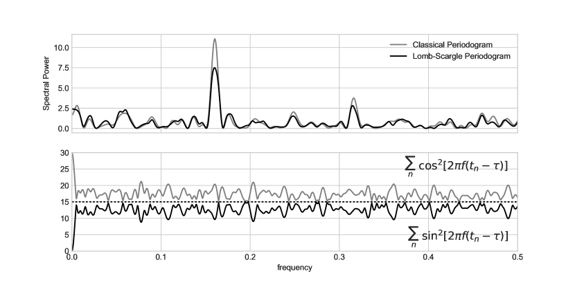
A remarkable feature of Scargle’s modified periodogram is that it is identical to the result obtained by fitting a model consisting of a simple sinusoid to the data at each frequency and constructing a “periodogram” from the goodness-of-fit at each frequency—an estimator which was considered in some depth by Lomb (1976). From this perspective, the shift defined in Equation 34 serves to orthogonalize the normal equations used in the least squares analysis. Partly due to this deep connection between Fourier analysis and least-squares analysis, the modified periodogram in Equation 33 has since become commonly referred to as the Lomb-Scargle Periodogram, although versions of this approach had been employed even earlier (see, e.g. Gottlieb et al., 1975).
Because of the close similarity between the classical and Lomb-Scargle periodograms, the bulk of or previous discussion applies—at least qualitatively—to periodograms computed with the Lomb-Scargle method. In particular, reasoning about the effect of window functions on the observed Lomb-Scargle power spectrum remains qualitatively useful even if it is not quantitatively precise.
One important caveat of the simple Lomb-Scargle formula is that the statistical guarantees only apply when the observations have uncorrelated white noise; data with more complicated noise characteristics must be treated more carefully; see, e.g., Vio et al. (2010) or the Least Squares approach discussed in Section 6.1.
6 The Least-Square Periodogram and its Extensions
The equivalence of the Fourier interpretation and least squares interpretation of the Lomb-Scargle periodogram allows for some interesting and useful extensions, some of which we will explore in this section. First, let’s consider the Least Squares periodogram itself.
In the least squares interpretation of the periodogram, a sinusoidal model is proposed at each candidate frequency :
| (35) |
where the amplitude and phase can vary as a function of frequency. These model parameters are fit to the data in the standard least-squares sense, by constructing the statistic at each frequency:
| (36) |
We can find the “best” model by minimizing at each freuqnecy with respect to and ; we will denote this minimum value as . Scargle (1982) showed that with this setup, the Lomb-Scargle periodogram from Equation 33 can be equivalently written:
| (37) |
where is the non-varying reference model. The key realization here is that the Lomb-Scargle periodogram essentially assumes a sinusoidal model for the data; this is visualized in LABEL:ls-model for the data we had seen in LABEL:LINEAR-data. This immediately begs the question: can we compute a “periodogram” based on more general forms of the above model to more effectively fit the data?

6.1 Measurement Errors
Perhaps the most important modification to the periodogram is to construct it such that it correctly handles measurement error in the data. This can be done through the standard change to the expression: i.e., if there are Gaussian errors on each observed , we can re-write Equation 36 in the following (standard) way:
| (38) |
The periodogram constructed from this definition will more accurately reflect the spectral power of noisy observations. The effect of this modification on Equation 33 is the addition of a multiplicative weight within each of the summations. Early versions of this sort of modification appeared in Gilliland & Baliunas (1987) and Irwin et al. (1989); Scargle (1989) derived this “weighted” form of the periodogram without direct reference to the least squares model, and Zechmeister & Kürster (2009) showed that such a modification does not change the statistical properties of the resulting periodogram.
This generalization of also suggests a convenient way to construct a periodogram in the presence of correlated observational noise. If we let denote the noise covariance matrix for observations, and construct the vectors
| (39) |
then the expression for correlated errors can be written
| (40) |
which reduces to Equation 38 if noise is uncorrelated (i.e., if the off-diagonal terms of are zero). This resulting periodogram is quite similar to the approach to correlated noise developed by Vio et al. (2010) from the Fourier perspective, and is in fact exactly equivalent in the case of the “zero-mean colored noise” example considered therein.
6.2 Data Centering and the Floating Mean Periodogram
Another commonly-applied modification of the periodogram has variously been called the Date-compensated Discrete Fourier Transform (Ferraz-Mello, 1981), the floating-mean periodogram (Cumming et al., 1999; VanderPlas & Ivezic, 2015), or the generalized Lomb-Scargle Method (Zechmeister & Kürster, 2009), and involves adding an offset term to the sinusoidal model at each frequency333We choose to follow Cumming et al. (1999) and VanderPlas & Ivezic (2015) and call this a “Floating Mean” model, to avoid confusion of the different uses of the term “generalized periodogram” in, e.g. Bretthorst (2001) and Zechmeister & Kürster (2009). :
| (41) |
This turns out to be quite important in practice, because the standard Lomb-Scargle approach assumes that the data are pre-centered around the mean value of the (unknown) signal. In many analyses, this requirement is accomplished by pre-centering data about the sample mean: this approach is generally robust when the data provide full phase coverage of the observed signal; however, due to selection effects and survey cadence, full phase coverage can not always be guaranteed. Using the sample mean in such cases can potentially lead to suppression of peaks of interest.

A simulated example of this is shown in Figure 22: the data consist of noisy observations of a sinusoidal signal in which the faintest observations are omitted from the dataset (due to, e.g., a detection threshold). Applying the standard Lomb-Scargle periodogram to pre-centered data leads to a periodogram that suppresses the true period of 0.3 days (lower right panel). Using the floating-mean model of Equation 41 yields a periodogram that identifies this true period (upper right panel). A detailed study of the floating-mean model is given by Zechmeister & Kürster (2009) who show that the addition of the floating mean term does not change the useful statistical properties outlined in Section 5.
6.3 Higher-order Fourier Models
A further generalization of the least squares periodogram involves multi-term Fourier models: rather than fitting just a single sinusoid at each frequency, we might fit a partial Fourier series, adding additional sinusoidal components at integer multiples of the fundamental frequency:
| (42) |
Bretthorst (1988) takes a comprehensive look at this type of multi-term extension to the periodogram, as well as related extensions to decaying signals and other more complex models.

This kind of Fourier series generalization to the periodogram is quite tempting, because it means that the periodogram can be tuned to fit models that are more complicated than simple sine waves. In some cases, this can be very useful; for example, LABEL:binary-multiterm shows a Lomb-Scargle analysis of an eclipsing binary star, characterized by both a primary and secondary eclipse. The standard Lomb-Scargle periodogram (upper panels) is maximized at twice the true rotation frequency, because the simple sinusoidal model is unable to closely fit the primary and secondary eclipses separately. A six-term Fourier model (lower panels) is sufficiently flexible that it can detect the true 17.5-hour period, though this comes at the expense of a much noisier periodogram.
This additional periodogram noise is easy to understand: in the least-squares view of the periodogram, the periodogram height at any frequency is directly related to how well the model fits the data. For nested linear models, adding additional terms will always provide an equal or better fit to data than the simpler model, and so it follows that a periodogram based on a more complex model will be higher at all frequencies, not just at frequencies of interest! Indeed, this effect can be readily observed in LABEL:binary-multiterm.

This background noise in the multi-term periodogram can also be understood in terms of aliasing. Consider LABEL:kepler-multiterm, which shows several multi-term fits to the Kepler data from LABEL:kepler-data. Given a standard periodogram with a peak or sub-peak at , a 2-term periodogram will duplicate this peak at , with the second harmonic driving the fit. Similarly, a 3-term periodogram will add additional peaks both at and , due to the original peak falling in the second and third harmonic. In general, you can expect an -term periodogram to contain aliases of every feature present in the standard periodogram; any strong peak revealed by the multi-term periodogram is due to two or more of these aliases coinciding.

In cases where the single-term power spectrum is itself noisy and/or dominated by partial aliasing due to window effects, these additional aliases can quickly wash-out any gains from the more complicated model. For example, consider the multi-term periodograms for the LINEAR data depicted in LABEL:LINEAR-multiterm: as previously discussed, the LINEAR periodogram contains a number of aliases of the true peak due to the dominant 1-day signal in the window function. Adding terms to this model only compounds this problem, increasing the number of spurious peaks at the low-frequency end. For data with even moderate levels of noise, chance coincidences of these peaks can lead to spurious detections which dominate the true peak, particularly for models with many Fourier terms.
6.4 Additional Extensions
When the periodogram is viewed from the least-squares model-fitting perspective, there is no need to limit the analysis to sums of sinusoids. There have been some very interesting applications extending this type of analysis to more arbitrary models. For example, periodogram models can be extended to measure decaying signals, non-stationary signals, multi-frequency signals, chirps, and other signal types (see, e.g. Jaynes, 1987; Bretthorst, 1988; Gregory, 2001). In particular, Bretthorst (1988) demonstrates the effectiveness of such approaches in applications ranging from medical imaging to astronomy. The challenge of such extensions is the fact that you often need to use some prior knowledge of the system being observed to decide whether a more complicated model is indicated, as well as what form of model to apply. In practice this comes up only when searching for very specific signals for which a more complicated model has some a priori physical motivation.
On the astronomy side, several examples of this flavor of extension exist. For example, the Supersmoother approach to detecting periodicity involves fitting a flexible non-parametric smoothing function to the data at each frequency (Reimann, 1994): the flexibility of the model leads to fewer aliasing issues when compared to the more constrained sinusoidal model. Another approach is to use empirically-derived templates as a functional fit at each frequency; this has been employed effectively in Sesar et al. (2010, 2013) and related work.
Finally, there has been some exploration of extensions to the Lomb-Scargle periodogram for use with multi-band observations, using various forms of regularization to control model complexity (VanderPlas & Ivezic, 2015; Long et al., 2016). With many of these least-squares and/or Bayesian extensions, computational complexity quickly becomes an issue, because fast approaches which can be used for sinusoidal fits (see Section 7.6) are not available for more general functional forms, though there is some promising work in this area: see, for example, the Fast Template Periodogram444http://ascl.net/code/v/1559 (Hoffman et al. 2017, in prep) which can quickly construct periodograms from Fourier approximations to templates.
6.5 A Note About “Bayesian” Periodograms
The least squares view of the Lomb-Scargle periodogram creates a natural bridge, via maximum likelihood, to Bayesian periodic analysis. In fact, Jaynes (1987) showed that the standard form of the Lomb-Scargle periodogram can be derived directly from the axioms of Bayesian probability theory outlined in his comprehensive treatment of the subject (Jaynes & Bretthorst, 2003)555Read this. Really.. In the Bayesian view, the Lomb-Scargle periodogram is in fact the optimal statistic for detecting a stationary sinusoidal signal in the presence of Gaussian noise.
For the standard, simple-sinusoid model, the Bayesian periodogram is given by the posterior probability of frequency given the data and sinusoidal model :
| (43) |
where is the Lomb-Scargle power from Equation 33. The effect of this exponentiation, as seen in LABEL:bayesian-periodogram, is to suppress side-lobes and alias peaks in relation to the largest one of the spectrum.

The benefit of the Bayesian approach is that it allows more flexible models, more principled treatment of nuisance parameters related to noise in the data, and the ability to make use of prior information in a periodic analysis. It explicitly returns probability density as a function of frequency, and it is tempting to think of this as the “natural” way to interpret the periodogram.
The problem, however, is that the Bayesian periodogram does not compute the probability that the data are periodic with a given frequency, but rather that probability conditioned on a relatively strong assumption: that the data are drawn from a sinusoidal model. As such, the standard Bayesian periodogram is not a useful measure of generic periodocity! In fact, the Baysian periodogram’s derivation under the assumption of a sinusoidal signal is perhaps the best argument against its use for unknown signals: the result of a Bayesian analysis is only ever as good as the assumptions that go into it, and for a general (not-necessarily sinusoidal) signal, those assumptions are incorrect, and the periodogram should not be trusted.
Now, the standard Lomb-Scargle periodogram can also be viewed as derived from a sinusoidal fit, and thus might appear subject to the same criticism. But unlike the Bayesian periodogram, the standard periodogram affords interpretation in light of Fourier analysis and window functions: here the incorrect sinusoidal model manifests itself in terms of frequency aliases, which can be understood through the analysis of window functions. In most cases of interest, such analysis turns out to be vital to the application and interpretation of the periodogram (see Section 7.2).
In other words, the Bayesian approach essentially goes “all-in” on the least squares interpretation of the periodogram, exponentially suppressing the information that allows you to reason about the periodogram in light of its connection to Fourier analysis. In contrived cases with clean sinusoidal data and unstructured window functions, exponential attenuation of side-lobes and aliases may seem appealing (see, e.g. Mortier et al., 2015), but that appeal extends to the real world only in the most favorable of cases—i.e., high signal-to-noise measurements of near-sinusoidal data with a very well-behaved survey window. In short, you shiould be wary of placing too much trust in a Bayesian periodogram, unless you’re certain of the type of signal you’re looking for.
This is not to say that all Bayesian approaches to periodic analysis are similarly flawed; there have been many interesting studies that go beyond the simple sinusoidal model and use more complex and/or flexible models. Some examples are models based on Fourier extensions with strong priors (e.g. Bretthorst, 1988), instrument-dependent parametric models (e.g. Angus et al., 2016), flexible non-parametric functions (e.g. Gregory & Loredo, 1992), Gaussian Process models (e.g. Wang et al., 2012), and specially-designed stochastic models (e.g. Kelly et al., 2014). Though these are often be more accurate and powerful than the Lomb-Scargle approach, they tend to be far more expensive computationally. Bayesian approaches based on Markov Chain Monte Carlo (MCMC) also tend to run into stability problems, particularly for multimodal or other complicated posterior distributions (See, for example, the RR Lyrae discussion in Kelly et al., 2014).
7 Practical Considerations when using Lomb-Scargle Periodograms
The previous sections have given a conceptual introduction to the Lomb-Scargle periodogram and its roots in both Fourier and Least-squares analysis. This section gets to the meat of the subject at hand: given this understanding of the Lomb-Scargle periodogram and related approaches, how should we use it most effectively in practice? The following sections will identify several of the important issues and questions that are not often addressed in the literature on the subject, but are nevertheless vital to consider when using the periodogram in practice.
7.1 Choosing a Frequency Grid
The frequency grid used for a Lomb-Scargle analysis is an important choice that is too-often glossed-over, probably because the choice is so straightforward in the more familiar case of uniformly-sampled data. For non-uniform data, it is not so simple, and there are two important considerations: the frequency limits and the grid spacing.
The frequency limit on the low end is relatively easy: for a set of observations spanning a length of time , a signal with frequency will complete exactly one oscillation cycle, and so this is a suitable minimum frequency. Often, it’s more convenient just to set this minimum frequency to zero, as it doesn’t add much of a computational burden and is unlikely to add any significant spurious peak to the periodogram.
The high-frequency limit is more interesting, and goes back to the discussion of Nyquist and/or limiting frequencies from Section 4.1: in order to not miss relevant information, it is important to compute the periodogram up to some well-motivated limiting frequency . This could be a true Nyquist limit based on the Eyer & Bartholdi (1999) definition, a pseudo-Nyquist limit based on careful scrutiny of the window function (cf. LABEL:kepler-data), a limiting frequency based on the integration time of individual observations, or a limit based on prior knowledge of the kinds of signals you expect to detect.

With the frequency range decided, we next must determine how finely to sample the frequencies between the limits. This choice turns out to be quite important as well: too fine a grid can lead to unnecessarily long computation times that can add up quickly in the case of large surveys, while too coarse a grid risks entirely missing narrow peaks that fall between grid points. For example, LABEL:LINEAR-coarse-grid shows the true, well-sampled periodogram (gray line), along with a periodogram computed for 10,000 equally-spaced periods covering the same range (black line). Because the spacing of the 10,000-point grid is much larger than the width of the periodogram peaks, the analysis entirely misses the most important peaks in the periodogram!
This shows us that it’s important to choose grid spacings smaller than the expected widths of the periodogram peaks. From our discussion of windowing in Section 3 (particularly LABEL:rectangular-window), we know that data observed through a rectangular window of length will have sinc-shaped peaks of width . To ensure that our grid sufficiently samples each peak, it is prudent to over-sample by some factor—say samples per peak—and use a grid of size . This pushes the total number of required periodogram evaluations to
| (44) |
So what is a good choice for ? Values ranging from (Schwarzenberg-Czerny, 1996; VanderPlas & Ivezic, 2015) to (Debosscher et al., 2007; Richards et al., 2012) seem to be common in the literature; for periodograms computed in this paper, we use .
Depending on the characteristics of the dataset, the size of the resulting frequency grid can vary greatly. For example, the Kepler data shown in LABEL:kepler-data has a pseudo-Nyquist frequency of and an observing window of . To compute five samples per peak thus requires evaluations of the periodogram. On the other hand, the LINEAR data shown in LABEL:LINEAR-data does not have any noteable aliasing structure in its window function. In this case the maximum detectable frequency is the Nyquist limit defined by its temporal resolution, which is 6 digits beyond the decimal point in days. From Equation 30, we can write , and given the observing window of , we find that five evaluations per peak across the entire detectable frequency range would require evaluations of the periodogram! Computing this large a periodogram in most cases is computationally intractable (see Section 7.6), and so in practice one must choose a smaller limiting frequency based on prior information about what kind of signals are expected in the data: for example, in LABEL:LINEAR-power, we chose a limiting frequency of based on typical oscillation periods expected for SX Phe-type stars. This leads to a much more manageable periodogram evaluations.
By comparison, data from the LSST survey (Ivezić et al., 2008) will fall somewhere in-between: full frequency coverage of the 10-year data up to a limiting frequency defined by the 30-second integration time for each visit would require roughly 25 million periodogram evaluations per object, which for fast implementations (see the next section) could be accomplished in several seconds on a modern CPU.
One final note: although it can be more easily interpretable to visualize periodograms as a function of period rather than a function of frequency, the peak widths are not constant in period. Regular grids in period rather than frequency tend to over-sample at large periods and under-sample at small periods; for this reason it is preferable to use a regular grid in frequency.
7.2 Failure Modes
When using the Lomb-Scargle periodogram in an observational pipeline, it is vital to keep in mind the failure modes of the periodogram approach, which are rooted in the aliasing and pseudo-aliasing effects rooted in the structure of the window function (recall Section 3). Due to the interaction of the signal, the convolution due to the survey window, and noise in the data, it is quite common for the largest peak in the periodogram to correspond not to the true frequency, but some alias of that frequency.
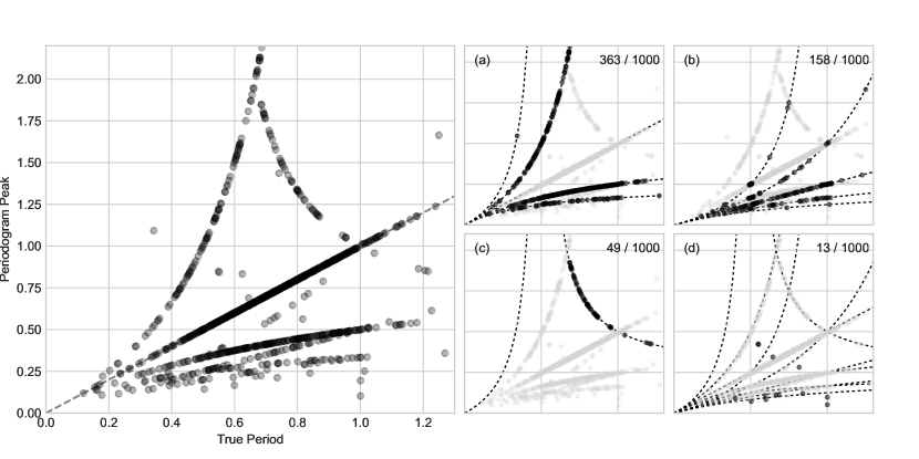
LABEL:failure-modes demonstrates this for some simulated data. The data consist of 60 noisy observations each of 1,000 simulated light curves within a span of 180 days. The window is typical of ground-based data, with each observation recorded within a few hours before or after midnight each night. The left panel shows the results: the peridogram peak coincides with the true period in under 50% of cases, and the modes of failure lead to noticeable patterns in the resulting plot. Though these are simulated observations, the pattern seen here is typical of real observations: see, for example, VanderPlas & Ivezic (2015) and Long et al. (2016) which show similar plots for RR Lyrae candidates from the Sloan Digital Sky Survey.
These patterns can be understood in terms of the interaction between the window function and the underlying spectral power. As we discussed in Section 3, a nightly observation pattern—typical of ground-based surveys—leads to a window function with a strong diurnal component that causes each frequency signature to be partially aliased at , for integers and cycle/day. (Recall Figures 17-18). This is the source of the failure modes depicted in panel (a) of LABEL:failure-modes; in terms of periods the above expression becomes:
| (45) |
where, to be clear, is a positive or negative integer and is the frequency of a strong feature in the window (here, cycle/day). For the simulated data, close to 36% of the objects are mis-characterized along these failure modes.
Another mode of failure is when the periodogram for an object with frequency isolates a higher harmonic of that fundamental frequency, such as . This may occur for periodic signals that are not strictly sinusoidal, and so have power at a higher harmonics. This higher harmonic peak is also subject to the same aliasing effects as in Equation 45. Thus we can extend Equation 45 and describe the failure modes depicted in panel (b) of LABEL:failure-modes with the following equation, for positive integers :
| (46) |
Panel (b) of LABEL:failure-modes illustrates this for ; this harmonic and its aliases account for roughly 15% of the results.
Panel (c) of LABEL:failure-modes shows the final pattern of failure in Lomb-Scargle results, which has an opposite trend with true period. This is closely related to the effects shown in panels (a) and (b), but comes from the even symmetry of the Lomb-Scargle periodogram. Every periodogram peak at frequency has a corresponding peak at , and this is true of aliases as well. If a peak’s aliases cross into the negative frequency regime, they are effectively reflected into the positive-frequency range. This reflection can be accounted for by a further modification of Equation 46—taking its absolute value:
| (47) |
Panel (c) shows the 5% of objects that fall along this reflected failure mode for , . After accounting for all these known sources of periodogram failure, only roughly 1% of points are misclassified in an “unexplained” way, seen in panel (d).
When applying a periodogram in practice, it is vital to take such effects into account, rather than blindly relying on the single periodogram peak as your best estimate of the period. Applying understanding of windowing and aliasing effects can help in detecting failures of the periodogram, but is no silver bullet. For an observed peak at from a survey whose window has strong power at , something like the following should probably be employed:
-
1.
Check for a peak at for at least . If a significant peak is found, then is probably an order- harmonic of the true frequency.666Notice that this step can detect aliases like those encoundered in LABEL:binary-multiterm, without resorting to a problematic multiterm model.
-
2.
Check for peaks at for at least (where is determined from plotting the survey window power, and is generally for ground-based surveys). If these aliases exist, then it is possible that you have found a peak on the sequence of expected aliases—though keep in mind that there is no way to know from the periodogram alone whether or not this is the “true” peak!
-
3.
For each of the top few of these aliases, fit a more complicated model (such as a multi-term Fourier series, template-based fit, etc.) to select among them.
For noisy observations, this procedure cannot generally guarantee that you have found the correct peak, but it is far preferable to the simplistic approach of blindly trusting the highest peak in the periodogram! We will come back to the question of uncertainty in the periodogram result in Section 7.4.
7.3 Window Functions and Deconvolution
Our discussion of window functions here and in Section 3 has highlighted the impact of structure in the survey window on the resulting observed power spectrum, and the importance of examining that window power to understand features of the resulting periodogram. Here we will consider the computation of the window function, as well as the possibility of recovering the true periodogram by deconvolving the window.
7.3.1 Computing the Window Function
The window power spectrum can be computed directly from the delta-function representation of the window function; From Equation 1, Equation 9, and Equation 27, we can write
| (48) |
Comparing this to Equation 26, we see that this is essentially the classical periodogram for data at all times . With this fact in mind, one convenient way to estimate the form of the window power is to compute a standard Lomb-Scargle periodogram on a series of unit measurements, making sure to not pre-center the data or to use a floating mean model. As Scargle (1982) notes, this computation does not give the true window—it differs from the true window just as the Lomb-Scargle periodogram differs from the classical periodogram—but in practice it is accurate enough to give useful insight into the window function’s important features. This method is how window power spectra has been computed throughout this paper.
7.3.2 Deconvolution and CLEANing
With this ability to compute the window function, we might hope to be able to use it quantitatively to remove spurious peaks from the observed power spectrum. Recall from Equation 28 that the observed data are a point-wise product of the underlying function and the survey window:
| (49) |
and the convolution theorem tells us that the observed Fourier transform is a convolution of the true transform and the window transform:
| (50) |
Given this relationship, we might hope to be able to invert this convolution to recover directly. For example, we could write:
| (51) | |||||
Because of the localization of observations, is zero for most values of and so and its Fourier transform are not well defined. Because of this, direct deconvolution is not an option in most cases of interest—in other words, the deconvolution problem is ill-posed and does not have a unique solution.
There have been a few attempts in the literature to use procedural algorithms to solve this under-constrained deconvolution problem, perhaps most notably by adapting the iterative CLEAN algorithm developed for deconvolution in the context of radio astronomy (Roberts et al., 1987). For cleaning of Lomb-Scargle periodograms, the CLEAN approach is hindered by three main deficiencies: first and most importantly, the CLEAN algorithm at each iteration assumes that the highest peak is the location of the primary signal; this is not always borne out for realistic observations of faint objects where the cleaning is most necessary (recall the discussion in Section 7.2). Second, the convolution takes place at the level of the Fourier transform rather than the PSD; trying to clean a PSD directly ignores important phase information. Third, the CLEAN algorithm assumes a classical FFT analysis: while the Lomb-Scargle periodogram is equivalent to classical periodogram in the limit of equally-spaced observations, it is not equivalent in the relevant case of unequal observations (see Section 5), and so any attempt to apply CLEAN to Lomb-Scargle analysis directly would be fundamentally flawed even if it were not ill-posed to begin with.
The latter two issues could be remedied by focusing on the non-uniform Fourier transform and the classical periodogram rather than the Lomb-Scargle modification, but doing so would jettison the benefits of Lomb-Scargle—i.e., its useful statistical properties and extensibility via least squares—and this would still not address the far more problematic first issue. My feeling is that there is room for a more principled approach to the unconstrained deconvolution problem for periodograms derived from non-uniform fast Fourier transforms (perhaps through some sort of L1/lasso regularization that imposes assumptions of sparsity on the true periodogram) but to date this does not appear to have been explored anywhere in the literature.
7.4 Uncertainties in Periodogram Results
An important aspect of reporting results from the Lomb-Scargle periodogram is the uncertainty of the estimated period. In many areas of science we are used to being able to report uncertainties in terms of errorbars, e.g. “the period is hours”. For periods derived from the Lomb-Scargle periodogram, however, uncertainties generally cannot be meaningfully expressed in this way: as we saw in the discussion of failure modes in Section 7.2, the concern for periodograms is more often a disjointed inaccuracy associated with false peaks and aliases, rather than a more smooth imprecision in location of a particular peak.
7.4.1 Peak Width and Frequency Precision
A periodic signal will be reflected in the periodogram by the presence of a peak of a certain width and height. In the Fourier view, the precision with which a peak’s frequency can be identified is directly related to the width of this peak; often the half-width at half-maximum is used. This can be formalized more precisely in the least squares interpretation of the periodogram, in which the inverse of the curvature of the peak is identified with the uncertainty (Ivezić et al., 2014)—which in the Bayesian view amounts to fitting a Gaussian curve to the (exponentiated) peak (Jaynes, 1987; Bretthorst, 1988). This introduces first-order dependence on the number of samples and their average signal-to-noise ratio ; the scaling is approximately (see, e.g. Gregory, 2001):
| (52) |
This dependence comes from the fact that the Bayesian uncertainty is related to the width of the exponentiated periodogram, which depends on , the height of the peak777 To see why, consider a periodogram with maximum value , so that . The Bayesian uncertainty comes from approximating the exponentiated peak as a Gaussian; i.e., . From this we can write or . In terms of signal-to-noise ratio , a well-fit model gives , which leads to the expression in Equation 52. .
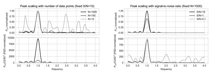
We have motivated from the Fourier window discussions that peak width is the inverse of the observational baseline; the surprising result is that to first order the peak width in the periodogram does not depend on either the number of observations or their signal-to-noise ratio! This can be seen visually in LABEL:peak-width-height, which shows periodograms for simulated data with a fixed 4-period baseline, with varying sample sizes and signal-to-noise ratios. In all cases, the widths of the primary peak are essentially identical, regardless of the quality or quantity of data! Data quality and quantity are reflected in the height of the peak in relation to the “background noise”, which speaks to the peak significance rather than the precision of frequency detection.
For this reason, if you insist on reporting frequency errorbars derived from peak width, the results can be pretty silly for observations with long baselines. For example, going by the peak width in LABEL:LINEAR-power, the periodogram reveals a period of hours, a relative precision of about 1/1000 percent. While this is an accurate characterization of the period precision assuming that peak is the correct one, it does not capture the much more relevant uncertainties demonstrated in Section 7.2, in which we might find ourselves on the wrong peak entirely. This is why in general, peak widths and Gaussian error bars should generally be avoided when reporting uncertainties in the context of a periodogram analysis.
7.4.2 False Alarm Probability
A much more relevant quantity for expressing uncertainty of periodogram results is the height of the peak, and in particular the height compared to the spurious background peaks that arise in the periodogram. LABEL:peak-width-height indicates that this property does depend on both the number of observations and their signal-to-noise ratio: for the small-/low signal-to-noise cases, the spurious peaks in the background become comparable to the size of the true peak. In fact, as we saw in Section 5, the ability to analytically define and quantify the relationship between peak height and significance is one of the primary considerations that led to the standard form of the Lomb-Scargle periodogram.
The typical approach to quantifying the significance of a peak is the False Alarm Probability (FAP), which measures the probability that a dataset with no signal would—due to coincidental alignment among the random errors—lead to a peak of a similar magnitude. Scargle (1982) showed that for data consisting of pure Gaussian noise, the values of the unnormalized periodogram in Equation 33 follows a distribution with two degrees of freedom; that is, at any given frequeny , if is the periodogram value from Equation 33, then
| (53) |
is the cumulative probability of observing a periodogram value less than , in data consisting only of Gaussian noise.888 Be aware that for different periodogram normalizations (See Section 7.5), the form of this distribution changes; see Cumming et al. (1999) or Baluev (2008) for a good summary of the statistical properties of various periodogram normalizations.
Independent Frequency Method
We are generally not interested in the distribution of one particular randomly-chosen frequency, but rather the distribution of the highest peak of the periodogram, which is a quite different situation.
By analogy, consider rolling a standard 6-sided die. The probability, in a single roll, of rolling a number, say is easy to compute: it’s 2 sides out of six, or . If, on the other hand, you roll 10 dice and choose the largest number among them, the probability that it will be greater than 4 is far larger than ; it is . The case for the periodogram is analogous: the probability of seeing a spurious peak at any single location (Equation 53) is relatively small, but the probability of seeing a single spurious peak among a large number of frequencies is much higher.
With the dice, this calculation is easy because the rolls are independent: the result of one roll does not affect the result of the next. With the periodogram, though, the value at one frequency is correlated with the value at other frequencies in a way that is quite difficult to analytically express—these correlations come from the convolution with the survey window. Nonetheless, one common approach to estimating the distribution has been to assume it can be modeled on some “effective number” of independent frequencies , so that the FAP can be estimated as
| (54) |
A very simple estimate for is based on our arguments of the expected peak width, . In this approximation, the number of independent peaks in a range is assumed to be . There have been various attempts to estimate this value more carefully, both analytically and via simulations (see, e.g. Horne & Baliunas, 1986; Schwarzenberg-Czerny, 1998; Cumming, 2004; Frescura et al., 2008), but all such approaches are necessarily only approximations.
Baluev (2008) Method
A more sophisticated treatment of the problem is that of Baluev (2008), who derived an analytic result based on theory of extreme values for stochastic processes. For the standard periodogram in Equation 33, Baluev (2008) showed that the following formula for the FAP provides a close upper-limit even in the case of highly structured window functions:
| (55) |
where, for the normalized periodogram (Equation 59),
| (56) |
and is an effective width of the observing window in units of the maximum frequency chosen for the analysis. This result is not an exact measure of the FAP, but rather an upper limit that is valid for alias-free periodograms, i.e. cases where the window function has very little structure, but which holds quite well even in the case of more realistic survey windows.
Bootstrap Method In the absence of a true analytic solution to the false alarm probability, we can turn to computational methods such as the bootstrap. The bootstrap method is a technique in which the statistic in question is computed repeatedly on many random resamplings of the data in order to approximate the distribution of that statistic (see Ivezić et al., 2014, for a useful general discussion of this technique). For the periodogram, in each resampling we keep the temporal coordinates the same, draw observations randomly with replacement from the observed values, and then compute the maximum of the resulting periodogram. For enough resamplings, the distribution of these maxima will approximate the true distribution for the case with no periodic signal present. The bootstrap produces the most robust estimate of the FAP because it makes few assumptions about the form of the periodogram distribution, and fully accounts for survey window effects.
Unfortunately, the computational costs of the bootstrap can be quite prohibitive: to accurately measure small levels of FAP requires constructing a large number of full periodograms. If you are probing a false positive rate of among bootstrap reseamples, you would roughly expect to find relevant peaks in your bootstrap sample. More concretely, for 1,000 bootstrap samples, you’ll find only peaks reflecting a 1% false positive rate. The random fluctuations in that count translate directly to an inability to accurately estimate the false positive rate at that level. A good rule-of-thumb is that to accurately characterize a false positive rate requires something like individual periodograms to be computed—this grows computationally intractable quite quickly. The bootstrap is also not universally applicable: for example, it does not correctly account for cases where noise in observations is correlated; for more discussion of the bootstrap approach and its caveats, see Ivezić et al. (2014) and references therein.
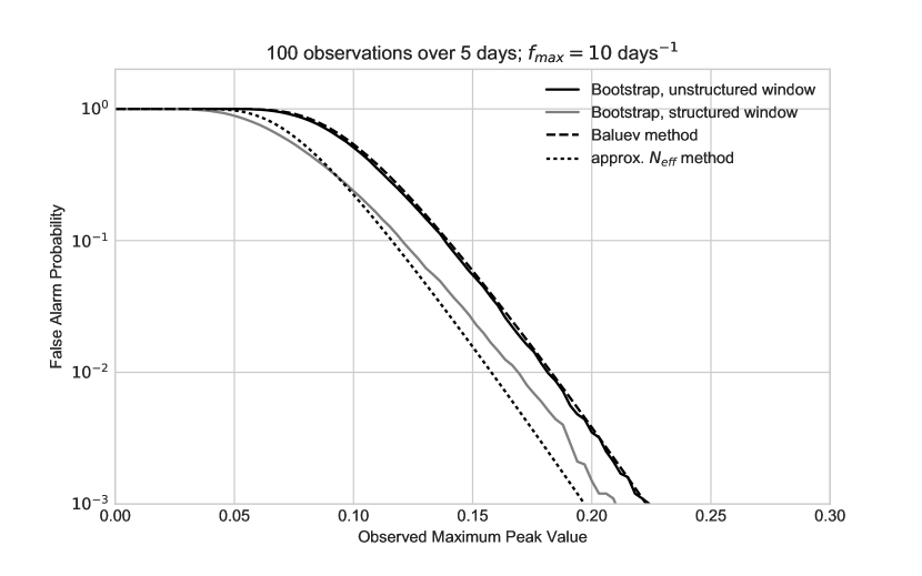
LABEL:FAP-bootstrap compares these methods of estimating the false alarm probability, for both an unstructured survey window, and a structured window which produces the kinds of aliasing we have discussed above. The naïve approximation in this case under-estimates the FAP at nearly all levels—so, for example, it might lead you to think a peak has a FAP of 10% when in fact it is closer to 30%. The Baluev method, by design, over-estimates the FAP, and is quite close to the bootstraped distribution in the case of an unstructured window. For a highly structured window, the Baluev method does not perform as well, but still tends to over-estimate the FAP—so, for example, it might lead you to think a peak as a FAP of 10% when in fact it is closer to 5%.
Finally, I will note that Suveges (2012) has shown the promise of a hybrid approach of the bootstrap method and the extreme value statistics of Baluev (2008); this has the ability to compute accurate FAPs without the need to compute thousands of full bootstrapped periodograms.
What Does the False Alarm Probability Measure?
While the False Alarm Probability can be a useful concept, you should be careful to keep in mind that it answers a very specific question: “what is the probability that a signal with no periodic component would lead to a peak of this magnitude?”. In particular, it emphatically does not answer the much more relevant question “what is the probability that this dataset is periodic given these observations?”. This boils down to a case of , but still it is common to see the false alarm probability treated as if it speaks to the second rather than the first question.
Similarly, the false alarm probability tells us nothing about the false negative rate; i.e. the rate at which we would expect to miss a periodic signal that is, in fact, present. It also tells us nothing about the error rate; i.e. the rate at which we would expect to identify an incorrect alias of a signal present in our data (as we saw in Section 7.2). Too often users are tempted to interpret the FAP too broadly, with the hope that it would speak to questions that are beyond its reach.
Unfortunately, there is no silver bullet for answering these broader, more relevant questions of uncertainty of Lomb-Scargle results. Perhaps the most fruitful path toward understanding of such effects for a particular set of observations—with particular noise characteristics and a particular observing window—is via simulated data injected into the detection pipeline. In fact, this type of simulation is a vital component of most (if not all) current and future time-domain surveys that seek to detect, characterize, and catalog periodic objects, regardless of the particular approach used to identify periodicity (see, e.g. Delgado et al., 2006; Ridgway et al., 2012; Ivezić et al., 2008; Sesar et al., 2010; Oluseyi et al., 2012; McQuillan et al., 2012; Drake et al., 2014, etc.)
7.5 Periodogram Normalization and Interpretation
Often it is useful to be able to interpret the periodogram values themselves. Recall that there are two equally valid perspectives of what the periodogram is measuring—the Fourier view and the least-squares view—and each of these lends itself to a different approach to normalizion and interpretation of the periodogram.
7.5.1 PSD normalization
When considering the periodogram from the Fourier perspective, it is useful to normalize the periodogram such that in the special case of equal spaced data, it recovers the standard Fourier power spectrum. This is the normalization used in Equation 33 and the equivalent least-squares expression seen in Equation 37:
| (57) |
For equally-spaced data, this periodogram is identical to the standard definition based on the fast Fourier transform:
| (58) |
in particular, this means that the units of the periodogram are , and can be interpreted as squared-amplitudes of the Fourier component at each frequency. Note, however, that the units change if data uncertainties are incorporated into the periodogram as in Section 6.1; the periodogram in this normalization becomes unitless: it is essentially a measure of periodic content in signal-to-noise ratio rather than in signal itself.
7.5.2 Least-squares normalization
In the least-squares view of the periodogram, the periodogram is interpreted as an inverse measure of the goodness-of-fit for a model. When we express the periodogram as a function of model fits as in Equation 57, it becomes clear that the periodogram has a mathematical maximum value: if the sinusoidal model perfectly fits the data at some frequency , then and the periodogram is maximized at a value of . On the other end, it is mathematically impossible for a best-fit sinusoidal model at any frequency to do worse than the simple constant, non-varying fit reflected in , and so the minimum value of Equation 57 is exactly zero.
This suggests a different normalization of the periodogram, where the values are dimensionless and lie between 0 and 1:
| (59) |
This “normalized periodogram” is unitless, and is directly proportional to the unnormalized (or PSD-normalized) periodogram in Equation 57.
While the normalization does not affect the shape of the periodogram, its main practical consequence is that the statistics of the resulting periodogram differ slightly, and this needs to be taken into account when computing analytic estimates of uncertainties and false alarm probabilities explored in Section 7.4.2. Other normalizations exist as well, but seem to be rarely used in practice. For a concise summary of several periodogram normalizations and their statistical properties, refer to the introduction of Baluev (2008).
7.6 Algorithmic Considerations
Given the size of the frequency grid required to fully characterize the periods from a given dataset, it is vital to have an efficient algorithm for evaluating the periodogram. We will see that the naïve implementation of the standard Lomb-Scargle formula (Equation 33) scales poorly with the size of the data, but that fast alternatives are available.
Suppose you have a set of observations over a time-span for an average cadence of . From Equation 44 we see that the number of frequencies we need to evaluate is . Holding constant the average survey cadence and , we find that the number of frequencies required is directly proportional to the number of data points. The computation of the Lomb-scargle periodogram in Equation 33 requires sums over sinusoids at each of the frequencies, and thus we see that the naïve scaling of the algorithm with the size of the dataset is , when survey properties are held constant. Due to the trigonometric functions involved, this turns out to be a rather “expensive” , which makes the direct implementation impractical for even modestly-sized datasets.
Fortunately, several faster implementations have been proposed to compute the periodogram to arbitrary precision in time. The first of these is discussed in Press & Rybicki (1989), which uses an inverse interpolation operation along with a Fast Fourier Transform to compute the trigonometric components of Equation 33 very efficiently over a large number of frequencies. Zechmeister & Kürster (2009) showed how this approach can be easily extended to the floating mean periodogram discussed in Section 6.2.
A qualitatively similar approach to the Press & Rybicki (1989) algorithm is presented by Leroy (2012): It makes use of the Non-equispaced Fast Fourier Transform (NFFT, see Keiner et al., 2009) to compute the Lomb-Scargle periodogram about a factor of 10 faster than the Press & Rybicki (1989) approach. For the multi-term models discussed in Section 6.3, Palmer (2009) presents an adaptation of the Press & Rybicki (1989) method that can compute the multi-term result in , for data points and Fourier components.
8 Conclusion and Summary
This paper has been a conceptual tour of the Lomb-Scargle periodogram, from its roots in Fourier analysis, to its equivalence with special cases of periodic analysis based on least squares model fitting and Bayesian analysis. From this conceptual understanding, we considered a list of challenges and issues to be considered when applying the method in practice. We will finish here with a brief summary of these practical recommendations, along with a somewhat opinionated post-script for further thought.
8.1 Summary of Recommendations
The previous pages contain a large amount of background and advice for working with the Lomb-Scargle periodogram. Following is a brief summary of the considerations to keep in mind when you apply this algorithm to a dataset:
-
1.
Choose an appropriate frequency grid: the minimum can be set to zero, the maximum set based on the precision of the time measurements (Section 4.1.2), and the grid spacing set based on the temporal baseline of the data (Section 7.1) so as to not sample too coarsely around peaks. If this grid size is computationally intractable, reduce the maximum frequency based on what kinds of signals you are looking for.
-
2.
Compute the window transform using the Lomb-Scargle periodogram, by substituting for each and making sure not to pre-center the data or use a floating-mean model (Section 7.3.1). Examine this window function for dominant features, such as daily or annual aliases (cf. LABEL:LINEAR-window) or Nyquist-like limits (cf. LABEL:kepler-data).
-
3.
Compute the periodogram for your data. You should always use the floating-mean model (Section 6.2), as it produces more robust periodograms and has few if any disadvantages. Avoid multi-term Fourier extensions (Section 6.3) when the signal is unknown, because its main effect is to increase periodogram noise (cf. Figures 24-25).
-
4.
Plot the periodogram, and identify any patterns that may be caused by features you observed in the window function power. Plot reference lines showing several False Alarm Probability levels to understand whether your periodogram peaks are significant enough to be labeled detections: use the Baluev method or the bootstrap method if it is computationally feasible (Section 7.4.2). Keep in mind exactly what the False Alarm Probability measures, and avoid the temptation to misinterpret it (Section 30).
-
5.
If the window function shows strong aliasing, locate the expected multiple maxima and plot the phased light curve at each. If there is indication that the sinusoidal model under-fits the data (cf. LABEL:binary-multiterm) then consider re-fitting with a multi-term Fourier model (Section 6.3).
-
6.
If you have prior knowledge of the shape of light curves you are trying to detect, consider using more complex models to choose between multiple peaks in the periodogram (Section 6.5). This type of refinement can be quite useful in building automated pipelines for period fitting, especially in cases where the window aliasing is strong.
-
7.
If you are building an automated pipeline based on Lomb-Scargle for use in a survey, consider injecting known signals into the pipeline to measure your detection efficiency as a function of object type, brightness, and other relevant characteristics (Section 7.2)
This list is certainly not comprehensive for all uses of the periodogram, but it should serve as a brief reminder of the kinds of issues you should keep in mind when using the method to detect periodic signals.
8.2 Postscript: Why Lomb-Scargle?
After considering all of these practical aspects of the periodogram, I think it is worth stepping back to revisit the question of why astronomers tend to gravitate toward the Lomb-Scargle approach rather than the (in many ways simpler) classical periodogram.
As discussed in Section 5, the Lomb-Scargle approach has two distinct benefits over the classical periodogram: the noise distribution at each individual frequency is chi-square distributed under the null hypothesis, and the result is equivalent to a periodogram derived from a least squares analysis. But somehow along the way, a mythology seems to have developed surrounding the efficiency and efficacy of the Lomb-Scargle approach. In particular, it’s common to see statements or implications along the lines of the following:
-
•
Myth: The Lomb-Scargle periodogram can be computed more efficiently than the classical periodogram. Reality: computationally, the two are quite similar, and in fact the fastest Lomb-Scargle algorithm currently available is based on the classical periodogram computed via the the NFFT algorithm (see Section 7.6).
-
•
Myth: The Lomb-Scargle periodogram is faster than a direct least squares periodogram because it avoids explicitly solving for model coefficients. Reality: model coefficients can be determined with little extra computation (see the discussion in Ivezić et al., 2014).
-
•
Myth: The Lomb-Scargle periodogram allows analytic computation of statistics for periodogram peaks. Reality: while this is true at individual frequencies, it is not true for the more relevant question of maximum peak heights across multiple frequencies, which must be either approximated or computed by bootstrap resampling (see Section 7.4)
-
•
Myth: The Lomb-Scargle periodogram corrects for aliasing due to sampling and leads to independent noise at each frequency. Reality: for structured window functions common to most astronomical applications, the Lomb-Scargle periodogram has the same window-driven issues as the classical periodogram, including spurious peaks due to partial aliasing, and highly correlated periodogram errors (see Section 7.2).
-
•
Myth: Bayesian analysis shows that Lomb-Scargle is the optimal statistic for detecting periodic signals in data. Reality: Bayesian analysis shows that Lomb-Scargle is the optimal statistic for fitting a sinusoid to data, which is not the same as saying it is optimal for finding the frequency of a generic, potentially non-sinusoidal signal (see Section 6.5).
With these misconceptions corrected, what is the practical advantage of Lomb-Scargle over a classical periodogram? What would we lose if we instead used the simple classical Fourier periodogram, estimating uncertainty, significance, and false alarm probability by resampling and simulation, as we must for Lomb-Scargle itself?
The advantage of analytic statistics for Lomb-Scargle evaporates in light of the need to account for multiple frequencies, so the only advantage left is the correspondence to least squares and Bayesian models, and in particular the ability to generalize to more complicated models where appropriate—but in this case you’re not really using Lomb-Scargle at all, but rather a generative Bayesian model for your data based on some strong prior information about the form of your signal. The equivalence of Lomb-Scargle to a Bayesian sinusoidal model is perhaps an interesting bit of trivia, but not itself a reason to use that model if your data is not known a priori to be sinusoidal—it could even be construed as an argument against Lomb-Scargle in the general case where the assumption of a sinusoid is not well-founded.
Conversely, if you replace your Lomb-Scargle approach with a classical periodogram, what you gain is the ability to reason quantitatively about the effects of the survey window function on the resulting periodogram (cf. Section 7.3.2). While the deconvolution problem is ill-posed, there is no reason to assume this is a fatal defect: ill-posed linear models are solved routinely in other areas of computational research, particularly by using sparsity priors or various forms of regularization. In any case, I would contend that there is ample room for practitioners to question the prevailing folk wisdom of the advantage of Lomb-Scargle over approaches based directly on the Fourier transform and classical periodogram.
8.3 Figures and Code
All computations and figures in this paper were produced using Python, and in particular used the Numpy (van der Walt et al., 2011; Oliphant, 2015), Pandas (McKinney, 2010), AstroPy (Astropy Collaboration et al., 2013), and Matplotlib (Hunter, 2007) packages. Periodograms where computed using the AstroPy implementations999The AstroPy Lomb-Scargle documentation is at http://docs.astropy.org/en/stable/stats/lombscargle.html of the Press & Rybicki (1989), Zechmeister & Kürster (2009), and Palmer (2009) algorithms, which were adapted from Python code originally published by Ivezić et al. (2014) and VanderPlas & Ivezic (2015). All code behind this paper, including code to reproduce all figures, is available in the form of Jupyter notebooks in the paper’s GitHub repository101010Source code & notebooks available at http://github.com/jakevdp/PracticalLombScargle/.
References
- Anderson (1971) Anderson, T. 1971, The statistical analysis of time series, Wiley series in probability and mathematical statistics: Probability and mathematical statistics (Wiley)
- Angus et al. (2016) Angus, R., Foreman-Mackey, D., & Johnson, J. A. 2016, ApJ, 818, 109
- Astropy Collaboration et al. (2013) Astropy Collaboration, Robitaille, T. P., Tollerud, E. J., et al. 2013, A&A, 558, A33
- Baluev (2008) Baluev, R. V. 2008, MNRAS, 385, 1279
- Bretthorst (1988) Bretthorst, G. 1988, Bayesian Spectrum Analysis and Parameter Estimation, Lecture Notes in Statistics (Springer)
- Bretthorst (2001) Bretthorst, G. L. 2001, in American Institute of Physics Conference Series, Vol. 568, Bayesian Inference and Maximum Entropy Methods in Science and Engineering, ed. A. Mohammad-Djafari, 241–245
- Bretthorst (2003) Bretthorst, G. L. 2003, Frequency estimation and generalized Lomb-Scargle periodograms, ed. E. D. Feigelson & G. J. Babu, 309–329
- Cumming (2004) Cumming, A. 2004, MNRAS, 354, 1165
- Cumming et al. (1999) Cumming, A., Marcy, G. W., & Butler, R. P. 1999, ApJ, 526, 890
- Debosscher et al. (2007) Debosscher, J., Sarro, L. M., Aerts, C., et al. 2007, A&A, 475, 1159
- Deeming (1975) Deeming, T. J. 1975, Ap&SS, 36, 137
- Delgado et al. (2006) Delgado, F., Cook, K., Miller, M., Allsman, R., & Pierfederici, F. 2006, in Society of Photo-Optical Instrumentation Engineers (SPIE) Conference Series, Vol. 6270, Society of Photo-Optical Instrumentation Engineers (SPIE) Conference Series, 1
- Drake et al. (2014) Drake, A. J., Graham, M. J., Djorgovski, S. G., et al. 2014, ApJS, 213, 9
- Dworetsky (1983) Dworetsky, M. M. 1983, MNRAS, 203, 917
- Edelson & Krolik (1988) Edelson, R. A., & Krolik, J. H. 1988, ApJ, 333, 646
- Eyer & Bartholdi (1999) Eyer, L., & Bartholdi, P. 1999, A&AS, 135, 1
- Ferraz-Mello (1981) Ferraz-Mello, S. 1981, AJ, 86, 619
- Foster (1996) Foster, G. 1996, AJ, 112, 1709
- Frescura et al. (2008) Frescura, F. A. M., Engelbrecht, C. A., & Frank, B. S. 2008, MNRAS, 388, 1693
- Gilliland & Baliunas (1987) Gilliland, R. L., & Baliunas, S. L. 1987, ApJ, 314, 766
- Gottlieb et al. (1975) Gottlieb, E. W., Wright, E. L., & Liller, W. 1975, ApJ, 195, L33
- Graham et al. (2013a) Graham, M. J., Drake, A. J., Djorgovski, S. G., Mahabal, A. A., & Donalek, C. 2013a, MNRAS, 434, 2629
- Graham et al. (2013b) Graham, M. J., Drake, A. J., Djorgovski, S. G., et al. 2013b, MNRAS, 434, 3423
- Gregory (2001) Gregory, P. C. 2001, in American Institute of Physics Conference Series, Vol. 568, Bayesian Inference and Maximum Entropy Methods in Science and Engineering, ed. A. Mohammad-Djafari, 557–568
- Gregory & Loredo (1992) Gregory, P. C., & Loredo, T. J. 1992, ApJ, 398, 146
- Hilditch (2001) Hilditch, R. W. 2001, An Introduction to Close Binary Stars, 392
- Horne & Baliunas (1986) Horne, J. H., & Baliunas, S. L. 1986, ApJ, 302, 757
- Huijse et al. (2012) Huijse, P., Estevez, P. A., Protopapas, P., Zegers, P., & Principe, J. C. 2012, IEEE Transactions on Signal Processing, 60, 5135
- Huijse et al. (2011) Huijse, P., Estevez, P. A., Zegers, P., Principe, J. C., & Protopapas, P. 2011, IEEE Signal Processing Letters, 18, 371
- Hunter (2007) Hunter, J. D. 2007, Computing In Science & Engineering, 9, 90
- Irwin et al. (1989) Irwin, A. W., Campbell, B., Morbey, C. L., Walker, G. A. H., & Yang, S. 1989, PASP, 101, 147
- Ivezić et al. (2014) Ivezić, Ž., Connolly, A., VanderPlas, J., & Gray, A. 2014, Statistics, Data Mining, and Machine Learning in Astronomy: A Practical Python Guide for the Analysis of Survey Data, Princeton Series in Modern Observational Astronomy (Princeton University Press)
- Ivezić et al. (2008) Ivezić, Ž., et al. 2008, arXiv:0805.2366
- Jaynes (1987) Jaynes, E. 1987, in Fundamental Theories of Physics, Vol. 21, Maximum-Entropy and Bayesian Spectral Analysis and Estimation Problems, ed. C. Smith & G. Erickson (Springer Netherlands), 1–37
- Jaynes & Bretthorst (2003) Jaynes, E. T., & Bretthorst, G. L., eds. 2003, Probability theory : the logic of science (Cambridge, UK, New York: Cambridge University Press)
- Keiner et al. (2009) Keiner, J., Kunis, S., & Potts, D. 2009, ACM Trans. Math. Softw., 36, 19:1
- Kelly et al. (2014) Kelly, B. C., Becker, A. C., Sobolewska, M., Siemiginowska, A., & Uttley, P. 2014, ApJ, 788, 33
- Koen (2006) Koen, C. 2006, MNRAS, 371, 1390
- Kolenberg et al. (2010) Kolenberg, K., Szabó, R., Kurtz, D. W., et al. 2010, ApJ, 713, L198
- Leroy (2012) Leroy, B. 2012, A&A, 545, A50
- Lomb (1976) Lomb, N. R. 1976, Ap&SS, 39, 447
- Long et al. (2016) Long, J. P., Chi, E. C., & Baraniuk, R. G. 2016, Ann. Appl. Stat., 10, 165
- McKinney (2010) McKinney, W. 2010, in Proceedings of the 9th Python in Science Conference, ed. S. van der Walt & J. Millman, 51 – 56
- McQuillan et al. (2012) McQuillan, A., Aigrain, S., & Roberts, S. 2012, A&A, 539, A137
- Mortier et al. (2015) Mortier, A., Faria, J. P., Correia, C. M., Santerne, A., & Santos, N. C. 2015, A&A, 573, A101
- Oliphant (2015) Oliphant, T. E. 2015, Guide to NumPy, 2nd edn. (USA: CreateSpace Independent Publishing Platform)
- Oluseyi et al. (2012) Oluseyi, H. M., Becker, A. C., Culliton, C., et al. 2012, AJ, 144, 9
- Palaversa et al. (2013) Palaversa, L., Ivezić, Ž., Eyer, L., et al. 2013, AJ, 146, 101
- Palmer (2009) Palmer, D. M. 2009, ApJ, 695, 496
- Percy (1986) Percy, J. R., ed. 1986, The Study of variable stars using small telescopes
- Press & Rybicki (1989) Press, W. H., & Rybicki, G. B. 1989, ApJ, 338, 277
- Press et al. (2007) Press, W. H., Teukolsky, S. A., Vetterling, W. T., & Flannery, B. P. 2007, Numerical Recipes 3rd Edition: The Art of Scientific Computing, 3rd edn. (New York, NY, USA: Cambridge University Press)
- Reimann (1994) Reimann, J. D. 1994, PhD thesis, University of California, Berkeley.
- Richards et al. (2012) Richards, J. W., Starr, D. L., Miller, A. A., et al. 2012, ApJS, 203, 32
- Ridgway et al. (2012) Ridgway, S. T., Chandrasekharan, S., Cook, K. H., et al. 2012, in Society of Photo-Optical Instrumentation Engineers (SPIE) Conference Series, Vol. 8448, Society of Photo-Optical Instrumentation Engineers (SPIE) Conference Series, 10
- Roberts et al. (1987) Roberts, D. H., Lehar, J., & Dreher, J. W. 1987, AJ, 93, 968
- Scargle (1982) Scargle, J. D. 1982, ApJ, 263, 835
- Scargle (1989) —. 1989, ApJ, 343, 874
- Scargle (1998) —. 1998, ApJ, 504, 405
- Scargle (2002) Scargle, J. D. 2002, in American Institute of Physics Conference Series, Vol. 617, Bayesian Inference and Maximum Entropy Methods in Science and Engineering, ed. R. L. Fry, 23–35
- Schuster (1898) Schuster, A. 1898, Terrestrial Magnetism, 3, 13
- Schwarzenberg-Czerny (1989) Schwarzenberg-Czerny, A. 1989, MNRAS, 241, 153
- Schwarzenberg-Czerny (1996) —. 1996, ApJ, 460, L107
- Schwarzenberg-Czerny (1998) —. 1998, MNRAS, 301, 831
- Schwarzenberg-Czerny (1999) —. 1999, ApJ, 516, 315
- Sesar et al. (2011) Sesar, B., Stuart, J. S., Ivezić, Ž., et al. 2011, AJ, 142, 190
- Sesar et al. (2010) Sesar, B., Ivezić, Ž., Grammer, S. H., et al. 2010, ApJ, 708, 717
- Sesar et al. (2013) Sesar, B., Grillmair, C. J., Cohen, J. G., et al. 2013, ApJ, 776, 26
- Stellingwerf (1978) Stellingwerf, R. F. 1978, ApJ, 224, 953
- Suveges (2012) Suveges, M. 2012, in Seventh Conference on Astronomical Data Analysis, ed. J.-L. Starck & C. Surace, 16
- Swingler (1989) Swingler, D. N. 1989, AJ, 97, 280
- van der Walt et al. (2011) van der Walt, S., Colbert, S. C., & Varoquaux, G. 2011, Computing in Science and Engg., 13, 22
- VanderPlas & Ivezic (2015) VanderPlas, J. T., & Ivezic, Z. 2015, ArXiv e-prints, arXiv:1502.01344
- Vetterli et al. (2014) Vetterli, M., Kovačević, J., & Goyal, V. K. 2014, Foundations of signal processing (Cambridge: Cambridge University Press)
- Vio et al. (2010) Vio, R., Andreani, P., & Biggs, A. 2010, A&A, 519, A85
- Wang et al. (2012) Wang, Y., Khardon, R., & Protopapas, P. 2012, ApJ, 756, 67
- Zechmeister & Kürster (2009) Zechmeister, M., & Kürster, M. 2009, A&A, 496, 577