Family-specific scaling laws in bacterial genomes.
Abstract
Among several quantitative invariants found in evolutionary genomics, one of the most striking is the scaling of the overall abundance of proteins, or protein domains, sharing a specific functional annotation across genomes of given size. The size of these functional categories change, on average, as power-laws in the total number of protein-coding genes. Here, we show that such regularities are not restricted to the overall behavior of high-level functional categories, but also exist systematically at the level of single evolutionary families of protein domains. Specifically, the number of proteins within each family follows family-specific scaling laws with genome size. Functionally similar sets of families tend to follow similar scaling laws, but this is not always the case. To understand this systematically, we provide a comprehensive classification of families based on their scaling properties. Additionally, we develop a quantitative score for the heterogeneity of the scaling of families belonging to a given category or predefined group. Under the common reasonable assumption that selection is driven solely or mainly by biological function, these findings point to fine-tuned and interdependent functional roles of specific protein domains, beyond our current functional annotations. This analysis provides a deeper view on the links between evolutionary expansion of protein families and the functional constraints shaping the gene repertoire of bacterial genomes.
I Introduction
As demonstrated by van Nimwegen vanNimwegen03 and confirmed by a series of follow-up studies Molina08 ; MOLINA09 ; cordero2009regulome ; Grilli2012 ; charoensawan2010genomic , striking quantitative laws exist for high-level functional categories of genes. Specifically, the number of genes within individual functional categories such as e.g. that of transcriptional regulators Stover2000 ; vanNimwegen03 ; Maslov2009 exhibit clear power-laws, when plotted as a function of genome size measured in terms of its number of protein-coding genes or, at a finer level of resolution, of their constitutive domains. In prokaryotes, such scaling laws appear well conserved across clades and lifestyles molina2009scaling , supporting the simple hypothesis that these scaling laws are universally shared by this group.
From the evolutionary genomics viewpoint Koonin2011 , these laws have been explained as a byproduct of specific “evolutionary potentials”, i.e., per-category-member rates of additions/deletions fixed in the population over evolution. As predicted by quantitative arguments, estimates of such rates correlate well with the category scaling exponents vanNimwegen03 ; Molina08 . A complementary point of view Maslov2009 ; Pang2011 ; Grilli2012 focuses on the existence of universal “recipes” determining ratios of proteins between different functions. Such recipes should mirror the “dependency structure” or network operating within genomes as well as other complex systems Pang2013 . According to this point of view the usefulness, and thus the occurence, of a given functional component depends on the presence of a set of other components, which are necessary for it to be operational.
Beyond functional categories, protein coding genes can be classified in “evolutionary families” defined by the homology of their sequences. Functional categories routinely contain genes from tens or more of distinct evolutionary families. The statistics of gene families also exhibits quantitative laws and regularities starting from a universal distribution of their per-genome abundance Huynen98 , explained by evolutionary models accounting for birth, death, and expansion of individual families Qian2001a ; Karev2004 ; Cosentino09 .
While some earlier work connects per-genome abundance statistics of families with functional scaling laws Grilli2012 , the link between functional category scaling and evolutionary expansion of gene families that build them remains relatively unexplored. Clearly, selective pressure is driven by functional constraints, and thus selection cannot in principle recognize families with identical functional roles. On the other hand, slight differences in the functional spectrum of different protein domains, and interdependency of different functions can make the scenario more complex. Thus, one central question is how the abundance of genes performing a specific function emerges from the evolutionary dynamics at the family level.
Two alternative extreme scenarios can be put forward: (i) the high-level scaling laws could emerge only at the level of functions, and be “combinatorially neutral” at the level of the evolutionary families building up a particular function, or, vice versa, (ii) they could be the result of the sum family-specific scaling laws. In the first scenario all or most of the families performing a particular function would be mutually interchangeable. In the second scenario, the evolutionary potentials would be family-specific and coincide with family evolutionary expansion rates, possibly emerging from the complex dependency structure cited above, and from fine-tuned functional specificity of distinct families. An intermediate possibility is that an interplay of constraints acts on both functional and evolutionary families. The first test for the feasibility of the second scenario is the existence of scaling laws for individual families. Here, focusing on bacteria, and using protein domains to define families, we present a clear evidence for family-specific scaling laws with genome size. We show that the abundance of the families follows power laws with genome size. Comparing functional categories with a suitable null model, we show that family-specific exponents may deviate significantly from the exponent of the associated functional category. We provide a comprehensive classification of families based on common scaling exponents, which recovers the known functional associations as well as revealing new ones, and may be used to detect possible misannotations. Finally, we develop quantitative tools to measure the heterogeneity of the scaling of families belonging to a given category or predefined group of families.
II MATERIALS AND METHODS
Data sources
We considered bacterial proteomes retrieved from the SUPERFAMILY (release 1.75 downloaded in October 2014, Gough01 ) and PFAM (release 27.0 downloaded in October 2014, bateman2004pfam ; Finn2014 ) database. Evolutionary families were defined from the domain assignments of 1535 superfamilies (SUPERFAMILY database) and 446 clans (PFAM database) on all protein sequences in completed genomes. We focused the analysis on the 1112 bacterial proteomes used as species reference in the SUPERFAMILY database. For the functional annotations of the SUPERFAMILY data, we considered annotation of SCOP domains as a scheme of 50 more detailed functional categories, mapped to 7 more general function categories, developed by C. Vogel vogel2006protein . PFAM clans were annotated on the same scheme of 50 functional categories, using the mapping of clans into superfamilies available from the PFAM website http://pfam.xfam.org/clan/browse#numbers finn2006pfam .
Data analysis
For each evolutionary domain family (or a functional category consisting of multiple evolutionary families), genome sizes (measured in the overall number of domains) were logarithmically binned. For each bin we calculated mean and standard deviation of the given family abundance (number of domains) within the bin. The estimated scaling exponent for family is the result of the non-linear least squares fitting of the binned data weighted by the standard error of family abundance. Genome size bins containing less than genomes were not taken into account. To filter out the data that, due to low-abundance or rare families, were affected by sampling problems, we considered three independent parameters, (i) the “occurrence”, i.e. the fraction of genomes where family is present, , where is the total number of genomes in the sample, and is the number of genomes where the family has non-zero abundance, (ii) the goodness of fit index
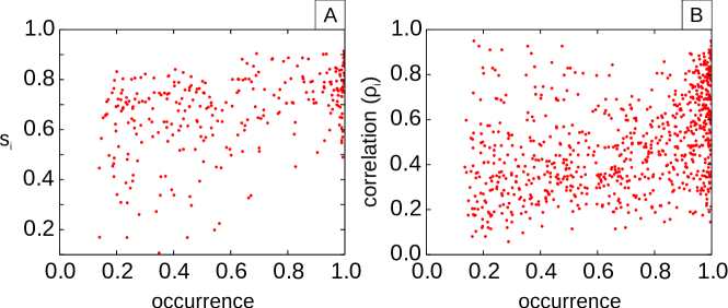
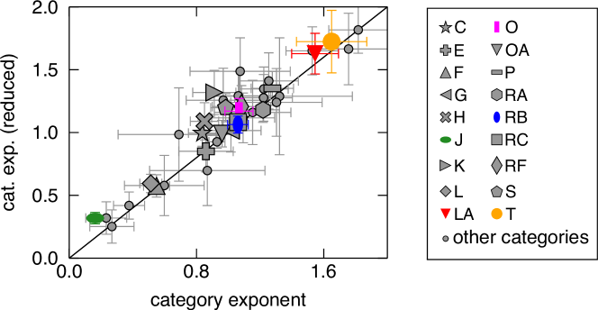
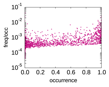
where is the error associated with the exponent , measured as the average squared deviation between the fit and the logarithm of the empirical abundance (see SI sec. S1), and (iii) the Pearson correlation coefficient between the logarithm of the family abundance and the logarithm of the genome size. The index puts on the same ground families with different exponents, but generally decreases as the scaling exponent increases, in accordance with the growth of fluctuations in families with higher exponents observed in ref. Grilli2014 . Hence, we decided to use it only for low exponents, where the Pearson correlation is a bad proxy of scaling. We considered families with and for exponents lower than 0.2, otherwise families with and reducing the dataset to 357 superfamilies and 178 clans that satisfy both requirements. As shown in Fig. S1A, and are not mutually correlated across the genomes, implying that the two requirements are in fact independent, the same is valid for and , see Fig. S1B. We verified that the removed families with the procedure described above do not influence the scaling of the category. Supplementary Fig. S2 reports the exponent of the category scaling before the thresholding (where all the families are considered) and after (where the domains belonging to the removed families are not considered in the category scaling), showing that the values are consistent for all the categories studied.
For each family within a given functional category, we defined a “heterogeneity score” as follows:
where and are,respectively, the scaling exponents of family and functional category . The heterogeneity measure for each functional category was defined as the average of the per-family heterogeneity scores :
where is the number of families in category .
The significance of the values found with this formula was assessed against a null model assuming that the total abundance of a category is distributed randomly across the associated families. The average abundance (i.e. the fraction of domains belonging to a family averaged over genomes) and occurrence (fraction of genomes where the family is present) of each family are both conserved (note that these two properties are uncorrelated in the data, hence we chose to conserve both in the null model, assuming that they are independent, see Supplementary Fig. S3).
Given a genome with elements in the functional category , divided into associated families, we redistributed the members among the sets conserving the average relative abundance of each family (see SI sec. S2). A member of family belonging to category was therefore added with probability
The resulting set of artificially built evolutionary categories constrains the occurrence pattern and the average abundance of the original ones. Scaling exponents for families in the null model are extracted with the procedure described above. Only functional categories containing domains from more than distinct families were compared to the null model. All procedures were implemented as custom Python 2.7 scripts.
III RESULTS
Families have individual scaling exponents, reflected by family-specific scaling laws
We started by addressing the question of whether individual families show scaling laws, and thus can be associated to specific scaling exponents. In order to do so, we isolated domains belonging to the same family across the sample of 1112 species-representative bacterial proteomes and plotted their abundance against the total number of domains in the corresponding proteome.
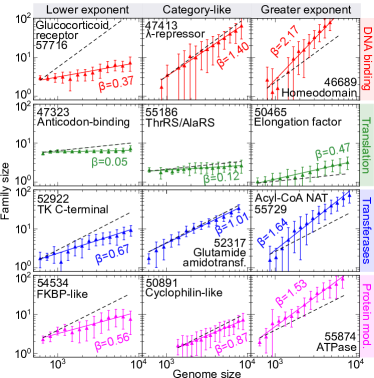
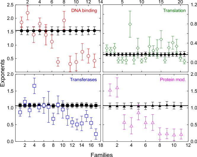
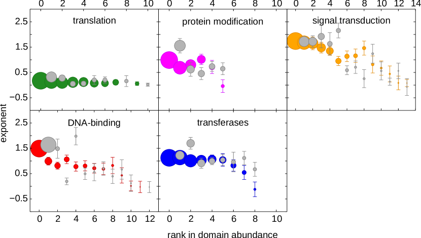
When the abundance is sufficiently high to overcome sampling problems, most families show a clearly identifiable individual scaling when plotted as a function of genome size. As an example, Fig. 1 shows the scaling of a set of chosen families in four selected functional categories. Additionally, some low-abundance families that occur in all genomes with a very consistent number of copies show definite scaling with exponents close to zero Grilli2014 , being clearly constant with size, with little or no fluctuations.
Given that functional categories follow specific scaling laws, likely related to function-specific evolutionary trends vanNimwegen03 ; Molina08 , there remain different open possibilities for the behavior of the evolutionary families composing the functional categories. One simple scenario is that family scalings are family-specific, thus validating the existence of family evolutionary expansion rates that are quantitatively different to the one of their functional category. In the opposite extreme scenario the scaling is only function-specific, and individual families performing similar functions are interchangeable. If this were the case, family diversity in scaling exponent would be only due to sampling effects, and the null model would fully reproduce the diversity in family scaling observed in empirical data. To address this question, we randomized the families within a category conserving their occurrence patterns and the category average abundance. The randomized families always show very similar scaling as the one of the corresponding category (see Supplementary Fig. S4). Hence, this analysis strongly supports the existence of family-specific scaling exponents that do not simply descend from the category scaling.
Fig. 1 shows that the presence of “outlier families” is common among functional categories. In most categories, we found families where the deviations from the category exponents is clear, beyond the uncertainty due to the errors from the fits. Fig. 1 shows some examples where in each of the shown categories may be higher, lower or comparable to . A table containing all the family and category exponents is available as supplementary information (Supplementary Table S1 and Table S2).
Finally, we considered the correlation of family scaling exponents with relevant biological and evolutionary parameters such as foldability (quantified by size-corrected contact order, SMCO Debes2013 ), the diversity of EC-numbers associated with families (quantifying the functional plasticity of a given family), selective pressure (quantified by the ratio of nonsynonimous to synonymous substitution rates Ndhlovu2015 ) and overall family abundance. The results are summarized in Supplementary Table S2. Foldability and appear to have little correlation with scaling exponents. Instead, we found a significant positive correlation of exponents with family abundance, and both quantities are correlated with diversity of EC-numbers in metabolic families. This suggests that, at least for metabolism, functional properties of a fold play a role in family scaling, and that beyond metabolism, abundance and scaling are, on average, not unrelated.
The heterogenetiy in scaling exponents is function-specific.
The analyses presented above support the hypothesis that functional categories contain families with specific scaling exponents. Indeed, the scaling exponents of the families can be significantly different from the category exponent with deviations that are much larger than predicted by randomizing the categories according to the null model (see Supplementary Fig. S4).
In order to quantify this “scaling heterogeneity” of functional categories, we computed for each family the distance between its scaling exponent and the category exponent (see Methods). We defined an index quantifying the heterogeneity of the scaling of the families within a category by averaging this distance over the families associated to a given category .
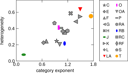
Figure 2A shows the relation between the heterogeneity and the category exponent . Interestingly, these two quantities are correlated, with categories with larger values of being more heterogeneous. This result can be intuitively rationalized in terms of the degrees of freedom imposed by the category exponent to the scaling of single families. Categories with small exponents are incompatible with extremely large fluctuations of family exponents, while categories with larger exponents can contain families with small . Indeed, this trend of heterogeneity with exponents is also observed in the null model, where the hetereogenity of null categories is much smaller than empirical ones, since all families tend to take the exponent category (Supplementary Fig. S4).
Figure 2B allows a direct comparison of the heterogeneity of different categories by subtracting the mean trend. It is noteworthy that the Signal Transduction functional category, which also has clear superlinear scaling, has much lower heterogeneity than DNA-binding/transcription factors. Among the categories with linear scaling, Transferases is one of the least heterogeneous ones, while the categories Protein Modification and Ion metabolism and Transport show a large variability in the exponents of the associated families. For Protein Modification, this signal is essentially due to the Gro-ES superfamily and to the HFSP90 ATP-ase domain, which have a clear superlinear scaling, while other chaperone families, such as FKBP, HSP20-like and J-domain are clearly sublinear with exponents close to zero. Interestingly, the Gro-EL domains, functionally associated to the Gro-EL, are part of this second class (exponent close to 0.2), showing very different abundance scaling to the Gro-EL partner domains. Conversely, the category Ion Metabolism and Transport is divided equally into linearly scaling (e.g., Ferritin-like Iron homeostasis domains) and markedly sublinear families, such as SUF (sulphur assimilation) / NIF (nitrogen fixation) domains. On the other hand, categories with small values of heterogeneity are made of families with exponents close to the one of the category, as shown in Table 1 in the case of, e.g., Transferases.

Determinants of the scaling exponent of a functional category
We have shown that scaling exponents of individual families may correspond to a vsriable extent to the exponent of the corresponding functional category. However, since categories are groups of families, the scaling of the former cannot be independent of the scaling of the latter. This section explores systematically the connection between the two. As detailed below, we find that in some cases the scaling exponent of functional categories is determined by few outlier families, while in other cases most of the families within a category contribute to the category scaling exponent.
While many families have a clear power-law scaling, functional categories may contain many low-abundance families with unclear scaling properties. When considered individually, these families do not contribute much to the total number of domains of a category, but their joined effect on the scaling of the category could be potentially important. Supplementary Fig. S5 shows that the sum of these low-abundance families does not suffer from sampling problems and shows a clear scaling. Interestingly, the scaling exponents for these sums once again does not necessarily coincide with the category exponents.
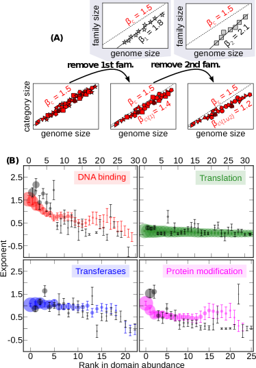
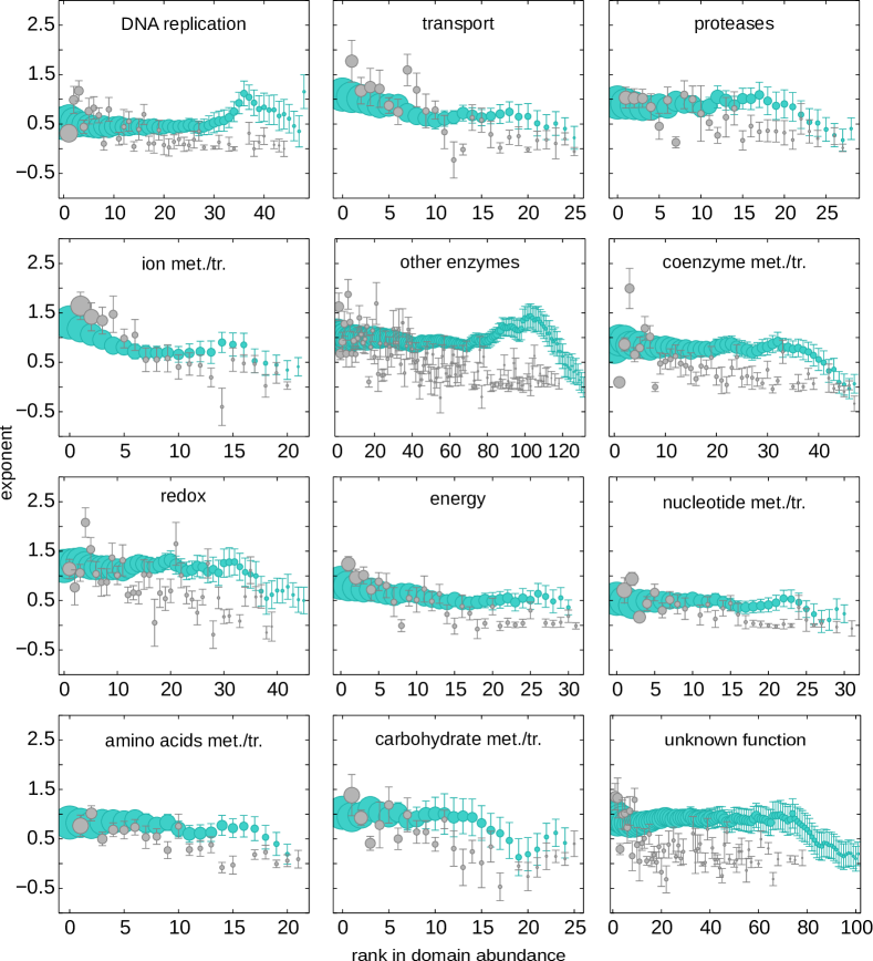
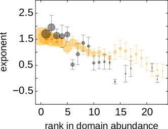
Figure 3A illustrates the systematic procedure that we used in order to understand how the scaling of categories emerges from the scaling of the associated families. Families were ranked by total abundance across all genomes (from the most to the least abundant) and removed one by one from the category. At each removal step in this procedure, both the scaling exponent of the removed family and the exponent of the remainder of the category are considered. In other words, the -th step evaluates the exponent of the -th ranking family (in order of overall abundance) and of the set of families obtained by removing the top-ranking families (with highest abundance) from the category. The resulting exponents quantify the contribution of each family to the global category scaling, as well as the collective contribution of all the families with increasingly lower overall abundance.
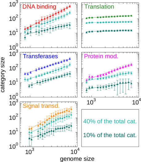
The results (Fig. 3B and Supplementary Fig. S6 and S7), show how the heterogeneity features described above are related to family abundance. The collective behavior of low-abundance families may deviate sensibly from that of the functional category and families follow scaling laws that sensibly deviate from the one of the corresponding functional categories. One notable example of this are Transcription-Factor DNA-binding domains. If the abundance of the outliers families is large enough in terms of the fraction of domains in the functional category, they might be responsible for determining the scaling of the entire category, as it happens in the case of DNA-binding (which is more extensively discussed in the following section).
Overall, one can distinguish between two main behaviors, either a category scaling is driven by a low number of highly populated “outlier” families (e.g. DNA binding and Protein Modification in Fig. 3B), or the category scaling is coherent, and robust to family subtraction (e.g. Transferases and Translation in Fig. 3B). While the first behavior appears to be more common for functional categories with higher scaling exponent, there are some exceptions. Notably, the scaling of strongly super-linear categories is not always driven by a few families. For example, the functional category Signal Transduction has an exponent , which remains stable after the removal of the largest families (Supplementary Fig. S5 and S7). Both behaviors are clearly visible for intermediate exponents (in order to appreciate this, compare the Transferases and Protein Modification categories in Fig. 3B).
Super-linear scaling of transcription factors is determined by the behavior of a few specific highly populated families.
We considered, in particular, the case of DNA-binding / transcription factors charoensawan2010genomic , which are known to exhibit peculiar scaling in bacteria Ranea2004 ; Maslov2009 . The abundance of domains in this functional category increases superlinearly (almost quadratically) with the total domain counts vanNimwegen03 ; Pang2011 ; Grilli2014 . As shown in the first row of Fig. 1B, not all the families in this functional category display a superlinear scaling charoensawan2010genomic , and the collective scaling of the low-abundance families with genome size is much slower (see Fig. 3 and Supplementary Fig. S5). Fig. 3B shows that only the most 5-6 abundant families display a super-linear scaling (). These are Winged helix DNA-binding domains (34.8% of abundance), Homeodomain-like (23.3 %) lambda repressor-like DNA-binding domains (9.5%) bipartite Response regulators (7.7%) Periplasmic binding protein-like (6.2%), and FadR-like (2.4%). The remaining 16.1% of the DNA-binding regulatory domains follows a clear sublinear scaling with genome size (exponent 0.7, see Supplementary Fig. S5).
Grouping families with similar scaling exponents shows known associations with biological function and reveals new ones.
The above analyses show that the range of scaling exponents of families within the same functional categories is generally wide and that the scaling behavior of some families sensibly deviates from their category. At the same time, functional categories show clear characteristic scaling laws, with well-defined exponents molina2009scaling . We, therefore, asked to what extent a range of family scaling exponents is peculiar to a functional category and how this compares to the category exponent . To this end, we grouped families based on their scaling exponents. We then used those groups to test how much specific range of exponents define specific functions by an enrichment test of functional annotations.
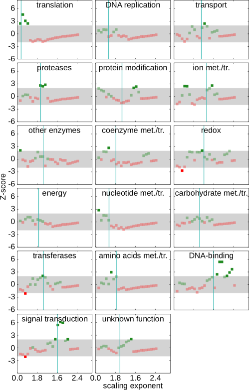
Table 1 shows that in most cases functional categories are over-represented in the exponent range where their scaling exponents is found. This confirms and puts in a wider perspective the previously reported strong association between abundance scaling with size and functional annotation. As can be expected from previous results, the functional category Protein Modification is an exception: this category is under-represented in the linear region even though its category exponent is , since it contains two strongly superlinear families and a bulk of families with sublinear scaling. This strong heterogeneity in scaling exponents is also visible in Fig. 3B.
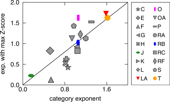
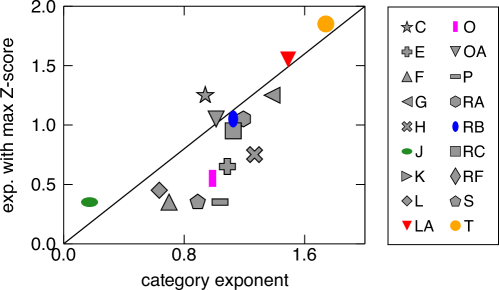
The results of this analysis are not sensitive to the chosen intervals for the scaling exponents. In order to show this, we performed a more systematic enrichment analysis, using sliding windows of exponents of width 0.4, and step 0.1, and plotting the Z-score for the enrichment as a function of the representative family exponent for each window (Supplementary Fig. S9). The maxima of this plot define a representative exponent for each functional category, and can be compared to the exponent measured directly from the plot of category abundance vs genome size (see Supplementary Figure S10). Interestingly, this analysis also shows that in many cases a single functional category is enriched for multiple groups of families with well-defined exponents, as in the case of the Protein Modification category. The cases of Ion Metabolism and Transport (already discussed), Coenzyme Metabolism and Transport, Redox also shows clear indications of enrichment for two or more exponent groups. For the category Coenzyme Metabolism and Transport this is due to the presence of a single abundant family with scaling exponent close to 2, the acyl-CoA dehydrogenase NM domain-like, whose functional annotation is still not well defined. In the case of Redox, the most abundant families (Thioredoxin-like, 4Fe-4S ferredoxins, Metallo-hydrolase/Oxydoreductase) scale linearly, but there is a wide range of families with exponents between 0.5 and 1, and once again two fairly abundant outlier families with superlinear scaling (Glyoxalase/Bleomycin resistance protein/Dioxygenase, and ALDH-like), both with a fairly wide range of functional annotations.
| Detailed function | ||||
|---|---|---|---|---|
| Translation | 20() | 1() | 0 | |
| DNA replication/repair | 11 | 7 | 0 | |
| Transport | 5 | 9 | 1 | |
| Proteases | 7 | 9 | 0 | |
| Protein modification | 8 | 1() | 2 | |
| Ion m/tr | 11 | 3 | 3() | |
| Other enzymes | 29 | 32 | 2 | |
| Coenzyme m/tr | 17() | 6 | 1 | |
| Redox | 4() | 18() | 2 | |
| Energy | 11 | 7 | 0 | |
| Nucleotide m/tr | 16() | 3() | 0 | |
| Carbohydrate m/tr | 4 | 8 | 0 | |
| Transferases | 5 | 11 | 1 | |
| Amino acids m/tr | 7 | 6 | 0 | |
| DNA-binding | 5 | 4 | 4() | |
| Signal transduction | 1() | 5 | 5() | |
| Unknown function | 9 | 7 | 0 |
IV DISCUSSION AND CONCLUSIONS
Our results gather a critical mass of evidence in the direction of family-specific expansion rules for the families of protein domains found in a genome. Although previous work had focused on individual transcription factor families charoensawan2010genomic , finding in some cases some definite scaling, no attempts were made to address this question systematically. The scaling laws for domain families appear to be very robust, despite of the limited sampling of families compared to functional annotations (which are super-aggregates of families and hence have by definition higher abundance). In particular, the results are consistent between the different classifications of families we tested (SUPERFAMILY and PFAM, see SI, sec. S4).
Overall, our results indicate that scaling laws are measurable at the family level, and, given the heterogeneous scaling of families with the same functional annotations, families are likely a more reliable description level for the scaling laws than functional annotations. The interpretation of these scaling laws is related to the evolutionary dynamics of family expansion by horizontal transfer or gene duplication, and gene loss Koonin2011 ; vanNimwegen03 ; Grassi2012 . Scaling exponents are seen as “evolutionary potentials” Molina08 , is based on a model of function-specific (multiplicative) family expansion rates. Assuming this interpretation, then our result that these rates may be different for different domain families having the same functional annotation may seem puzzling. Clearly, selective pressure can only act at the functional level, and if two folds were functionally identical, there should be reasonably no advantage selecting one with respect to the other, and doing so at different specific rates. For example, a transcription factor using one fold to bind DNA rather than another one should be indistinguishable from one using a different fold, provided binding specificity and regulatory action are the same.
In view of these considerations, we believe that our findings support a more complex scenario for the interplay between domain families and their functions. Specifically, we put forward two complementary rationalizations, both of which are probably in part verified in the data. The first is that functional annotations group together different domains whose abundance is linked in different ways to genome size because of their different biochemical and biological functional roles. Such differences may range from slight biochemical specificities of different folds to plain misannotations. This is possible, e.g., with enzymes, where the biochemical range of two different folds is generally different. This obervation might be related to the positive correlation we found between the number of EC numbers corresponding to a metabolic domain and its scaling exponent. However, such interpretation might be less likely applicable to, e.g., transcription factor DNA-binding domains, where functional annotation is fairly straightforward Babu03 , but different scaling behaviors with genome size are nevertheless found.
The second potential explanation assumes the point of view where scaling laws are the result of functional interdependency between different domain families Maslov2009 ; Grassi2012a , then correlated fluctuations around the mean of family pairs should carry memory of such dependency structures Pang2013 . More in detail, there may be specific dependencies connecting the relative proportions of domains with both different and equal functional annotations that are present in the same genome, which might determine the family-specific behavior Grilli2012 . While further analysis is required to elucidate these trends, we believe that gaining knowledge on functional dependencies would be an important step to understand the functional design principles of genomes.
Of notable importance is the case of the superlinear scaling of transcription factors, which has created notable debate in the past Ranea2005 ; Maslov2009 . For the first time, we look into how this trend is subdivided between the different DBDs Babu03 . Our analysis indicates that the superlinear scaling is driven by the few most abundant superfamilies (mostly winged-helix, homeodomain, lambda repressor). However, the remaining 10-20% of the functional category gives a clear sublinear scaling with genome size, which emerges beyond any sampling problems. We speculate that these other regulatory DNA-binding domains may be functionally different or behave differently over evolutionary time scales. Hence, the scaling of transcription factors with size in bacteria is driven by a small set of domain families with scaling exponent close to two, which take up most of the abundance, but does not appear to be peculiar of all transcription factors. A “toolbox” model considering the role of transcription factors as regulator of metabolic pathways and the finite universe of metabolic reactions Maslov2009 ; Pang2011 predicts scaling exponents close to two for transcription factor families. According to our results, such model should be applicable to the leading TF families. Interestingly, the heterogeneity in the behavior in transcription factor DNA-binding domains is much higher than that of the other notable superlinear functional category, signal transduction, where removal of the leading families does not significantly affect the observed scaling of abundance with genome size. Given the clarity and uniformity of the scaling exponent, we speculate that possibly a toolbox-like model may be applicable to understand the overall scaling of this category.
Other categories clearly contain multiple sets of families with coherent exponents or single outlier families. In some cases, two main groups of families with different scaling behavior clearly emerge, and higher observed scaling exponents may be related to a wider range of functional annotations. We propose that such easily detectable trends can be used to revise and refine functional annotations of protein domains. Such functional annotations are currently largely curated by humans, and based on subjective and/or biased criteria. The analysis of family scaling gives an additional objective test to define the coherence of the families that are annotated under the same function. While yet-to-be-developed automated inference methods based on our observations could serve this purpose, the quantitative scores defined here already provide useful information. The heterogeneity of a functional category is an indication of how likely that group of domain families follows a coherent expansion rate over evolution. The enrichment scores for sets of families with a given range of scaling exponent helps to pinpoint the sets of families within the functional category that expand coherently with genome size.
V ACKNOWLEDGEMENTS
We thank Erik van Nimwegen, Madan Babu, Otto Cordero and Purushottam Dixit for helpful discussions.
References
- (1) van Nimwegen, E. (2003) Scaling laws in the functional content of genomes. Trends in Genetics, 19(9), 479 – 484.
- (2) Molina, N. and van Nimwegen, E. (2008) The evolution of domain-content in bacterial genomes. Biology Direct, 3(1), 51.
- (3) Molina, N. and van Nimwegen, E. (jun, 2009) Scaling laws in functional genome content across prokaryotic clades and lifestyles.. Trends in genetics : TIG, 25(6), 243–7.
- (4) Cordero, O. X. and Hogeweg, P. (2009) Regulome size in Prokaryotes: universality and lineage-specific variations. Trends Genet,.
- (5) Grilli, J., Bassetti, B., Maslov, S., and Cosentino Lagomarsino, M. (Jan, 2012) Joint scaling laws in functional and evolutionary categories in prokaryotic genomes.. Nucleic Acids Res, 40(2), 530–540.
- (6) Charoensawan, V., Wilson, D., and Teichmann, S. A. (2010) Genomic repertoires of DNA-binding transcription factors across the tree of life. Nucleic acids research, 38(21), 7364–7377.
- (7) Stover, C., Pham, X., Erwin, A., Mizoguchi, S., Warrener, P., Hickey, M., Brinkman, F., Hufnagle, W., Kowalik, D., Lagrou, M., et al. (2000) Complete genome sequence of Pseudomonas aeruginosa PAO1, an opportunistic pathogen. Nature, 406(6799), 959–964.
- (8) Maslov, S., Krishna, S., Pang, T. Y., and Sneppen, K. (Jun, 2009) Toolbox model of evolution of prokaryotic metabolic networks and their regulation.. Proc Natl Acad Sci U S A, 106(24), 9743–9748.
- (9) Molina, N. and van Nimwegen, E. (2009) Scaling laws in functional genome content across prokaryotic clades and lifestyles. Trends in genetics, 25(6), 243–247.
- (10) Koonin, E. V. (Aug, 2011) Are there laws of genome evolution?. PLoS Comput Biol, 7(8), e1002173.
- (11) Pang, T. Y. and Maslov, S. (May, 2011) A toolbox model of evolution of metabolic pathways on networks of arbitrary topology.. PLoS Comput Biol, 7(5), e1001137.
- (12) Pang, T. Y. and Maslov, S. (Apr, 2013) Universal distribution of component frequencies in biological and technological systems.. Proc Natl Acad Sci U S A, 110(15), 6235–6239.
- (13) Huynen, M. and van Nimwegen, E. (1998) The frequency distribution of gene family sizes in complete genomes. Mol Biol Evol, 15(5), 583–589.
- (14) Qian, J., Luscombe, N. M., and Gerstein, M. (Nov, 2001) Protein family and fold occurrence in genomes: power-law behaviour and evolutionary model.. J Mol Biol, 313(4), 673–681.
- (15) Karev, G. P., Wolf, Y. I., Berezovskaya, F. S., and Koonin, E. V. (Sep, 2004) Gene family evolution: an in-depth theoretical and simulation analysis of non-linear birth-death-innovation models.. BMC Evol Biol, 4, 32.
- (16) Cosentino Lagomarsino, M., Sellerio, A., Heijning, P., and Bassetti, B. (2009) Universal features in the genome-level evolution of protein domains. Genome Biology, 10(1), R12.
- (17) Gough, J., Karplus, K., Hughey, R., and Chothia, C. (2001) Assignment of homology to genome sequences using a library of hidden Markov models that represent all proteins of known structure. Journal of Molecular Biology, 313(4), 903 – 919.
- (18) Bateman, A., Coin, L., Durbin, R., Finn, R. D., Hollich, V., Griffiths-Jones, S., Khanna, A., Marshall, M., Moxon, S., Sonnhammer, E. L., et al. (2004) The Pfam protein families database. Nucleic acids research, 32(suppl 1), D138–D141.
- (19) Finn, R. D., Bateman, A., Clements, J., Coggill, P., Eberhardt, R. Y., Eddy, S. R., Heger, A., Hetherington, K., Holm, L., Mistry, J., Sonnhammer, E. L. L., Tate, J., and Punta, M. (2014) Pfam: the protein families database. Nucleic Acids Research, 42(D1), D222–D230.
- (20) Vogel, C. and Chothia, C. (2006) Protein family expansions and biological complexity. PLoS Comput Biol, 2(5), e48.
- (21) Finn, R. D., Mistry, J., Schuster-Böckler, B., Griffiths-Jones, S., Hollich, V., Lassmann, T., Moxon, S., Marshall, M., Khanna, A., Durbin, R., et al. (2006) Pfam: clans, web tools and services. Nucleic acids research, 34(suppl 1), D247–D251.
- (22) Grilli, J., Romano, M., Bassetti, F., and Cosentino Lagomarsino, M. (jun, 2014) Cross-species gene-family fluctuations reveal the dynamics of horizontal transfers.. Nucleic acids research, 42(11), 6850–60.
- (23) Debes, C., Wang, M., Caetano-Anolles, G., and Graeter, F. (2013) Evolutionary optimization of protein folding.. PLoS Comput Biol, 9(1), e1002861.
- (24) Ndhlovu, A., Durand, P. M., and Hazelhurst, S. (2015) EvoDB: a database of evolutionary rate profiles, associated protein domains and phylogenetic trees for PFAM-A. Database, 2015, bav065.
- (25) Ranea, J. A. G., Buchan, D. W. A., Thornton, J. M., and Orengo, C. A. (Feb, 2004) Evolution of protein superfamilies and bacterial genome size.. J Mol Biol, 336(4), 871–887.
- (26) Grassi, L., Caselle, M., Lercher, M. J., and Cosentino Lagomarsino, M. (Mar, 2012) Horizontal gene transfers as metagenomic gene duplications.. Mol Biosyst, 8(3), 790–795.
- (27) Madan Babu, M. and Teichmann, S. (2003) Evolution of transcription factors and the gene regulatory network in Escherichia coli.. Nucleic Acids Res, 31, 1234–1244.
- (28) Grassi, L., Grilli, J., and Cosentino Lagomarsino, M. (May, 2012) Large-scale dynamics of horizontal transfers.. Mob Genet Elements, 2(3), 163–167.
- (29) Ranea, J. A. G., Grant, A., Thornton, J. M., and Orengo, C. A. (Jan, 2005) Microeconomic principles explain an optimal genome size in bacteria.. Trends Genet, 21(1), 21–25.
Supplementary Material for De Lazzari et al.
The scaling laws in the bacterial genomic repertoires are
family-specific.
Eleonora de Lazzari, Jacopo Grilli, Sergei Maslov and Marco Cosentino Lagomarsino
Supplementary Notes
S1 Filters for reliable family scaling
Many domain families are found only in a few genomes and/or in very few copies. For this reason, they might not show clear scaling properties. We excluded such families from the analysis with some filtering criteria. In order to filter out these families, we used three independent parameters. The first one is the occurrence of a family (i.e., the fraction of genomes where it is present, and the number of points available for the fit), the second one is the Pearson correlation of its abundance with genome size and the third one is the goodness of fit to a power law.
The occurence of the family is defined as
| (1) |
while is the number of genomes in which family is present and is the total number of genomes in the sample.
The Pearson correlation coefficient between the logarithm of the family abundance and the logarithm of the genome size quantifies the existence of a relation between family abundance and genome size. It should be noted that this quantity differs from : these two properties are not correlated in the data (Fig. S1B), which indicates that filters on their value should be applied independently.
Considering families with clear but shallow scaling or constant abundance across genomes, the Pearson correlation index gives values close to zero, or slighlty negative, therefore another parameter is required to assess the accuracy of the fit results. For each family whose estimated scaling exponent is lower than 0.2, we defined the quantity as
where is the logarithm of the empirical abundance of family and is the abundance calculated with the fit parameters, i.e.,
The goodness of fit index was defined as
so that the values of close to 1 correspond to the minimum value of the average squared deviation between the fit and the empirical values. The goodness of fit index is independent from the occurrence as shown in Fig. S1A.
We considered only the families with . If the fitted scaling exponent is higher than then we excluded the families with , while, for exponents lower than , only families with were taken into account. After this thresholding, we removed 1179 families out of 1536. While the fraction of such small and sparse families is large, we verified that they do not contribute significantly to the category scaling (see Figure S2).
S2 Formulation of the null model for family-specific scaling
The null model assumes that the total abundance of a category is distributed randomly across the families belonging to it. Both the average relative abundance (i.e. fraction of domains belonging to a family averaged over genomes) and occurrence (fraction of genomes where the family is present) of each family are conserved (they are in fact two independent properties, see Fig. S3).
The null model is based on the following ingredients.
-
•
The number of domains belonging to a category in genome , , is conserved.
-
•
For each genome, domains are not assigned to families that are not present in that genome.
-
•
The average frequency for each family with respect to the category is conserved.
The average frequency of the family with respect to the category is defined as
| (2) |
where the family index belongs to the set in category and the sum over is carried over all the genomes, while is the number of genomes in which family is present, is the abundance of family in genome and is the abundance of category in genome .
Given a genome , each realization of the null model redistributes randomly the domains of the functional category arranged in the families belonging to category in genome . Each one of the domains is assigned to family with probability
| (3) |
S3 Enrichment analysis for functional categories and families with similar scaling exponent
All families passing the filters described in section S1 were divided into three groups based on the values of their exponent :
-
•
sub-linearly scaling families,
-
•
linearly scaling families,
-
•
super-linearly scaling families,
We used hypergeometric tests to asses over- or under-representation of functional categories in these family groups. Given that is the number of families that belong to the category , is the number of families in either of the three groups defined above and is the total number of families involved in this analysis, the mean and the variance of the hypergeometric distribution are:
For each combination of functional category and family group, the quantity is the number of families that lie in the intersection of category with family group . The functional category is under-represented in the group if , over-represented if , where is the Z-score:
The resulting intersection values and the significant Z-scores are reported in Table 1 of the main text.
In order to prove that the results are independent from the chosen interval of the exponents, we substituted the three groups with sliding intervals of amplitude 0.4 and step 0.1 and repeated the same process. Only intervals with more than 10 families are considered. Fig. S9 shows that the results are consistent with the previous analysis. Fig. S10 shows how the exponent corresponding to the maximum Z-score differs in some cases from the category exponent.
S4 Main results hold also for PFAM clans
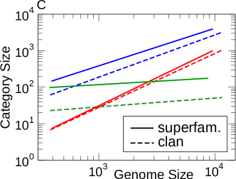
We chose PFAM clans as an alternative database to test our results. PFAM clans were annotated on the same scheme of 50 functional categories used for superfamilies, using the mapping of clans into superfamilies available from the PFAM website http://pfam.xfam.org/clan/browse#numbers finn2006pfam . The scaling laws for functional categories are recovered also for clans (Fig. S11 and Table LABEL:tab:TableS1cat) and are consistent with previous results vanNimwegen03 ; Molina08 ; MOLINA09 ; cordero2009regulome ; Grilli2012 ; charoensawan2010genomic .
The following main results were recovered for Pfam clans.
-
•
For each clan, the abundance across genomes scaleS as a power law of the genome size. Equally to SCOP superfamilies, Pfam clans have individual scaling exponents that may or may not follow the one of the associated functional category (Table. LABEL:tab:TableS2clan). The fitting method and threshold values are the same used for supefamilies (sec. S1). 178 clans out of 446 passed the filters and were employed for further analysis.
-
•
The heterogeneity (average of the distance between the category exponent and the clan exponent), positively correlates with the category exponent (Fig. S12). Functional categories with superlinear scaling tend to be more heterogeneous and, as found for superfamilies, the functional category Signal Transduction is less heterogeneous than DNA-binding, although having the largest exponent. Unlike the case of superfamilies, Protein Modification does not have high heterogeneity score, but the difference in scaling between the (strongly superlinear) outlier family Gro-ES and the remaining ones is observed. For clans, the scaling of Protein Modification is once again strongly biased by the clan “GroES-like superfamily” (20% of the total domains).
-
•
Either few or most of the clans determine the scaling exponent of the functional category they belong to. Figure S8 is coherent with what observed for superfamilies, in particular the functional category of DNA-binding is dominated by one clan (the “Helix-turn-helix” clan) that accounts for 83% of the total domains. As for superfamilies, Signal Trasduction is robust to the progressive removal of families confirming that the presence of dominant clans is not related to the superlinear scaling of the category.
-
•
Grouping clans with similar scaling exponents recovers known associations between the category exponent and the biological function (Fig. S13).
S5 Correlation between family scaling and EC numbers
The Enzyme Commission (EC) number is a classification scheme for enzyme-catalyzed chemical reactions. It is built as a four-levels tree where the top nodes are six main groups of reactions, namely Oxidoreductases, Transferases, Hydrolases, Lyases, Isomerases and Ligases. We used the mapping between Superfamilies and EC terms Gough01 , to investigate the correlation between the Superfamily scaling and the number of different reactions in which the family is involved. This quantity is the count of distinct EC numbers corresponding to the finest level of the EC classification. This number shows a positive correlation (Spearman 0.74) with the scaling exponent of metabolic family (see Table S2). The diversity of EC numbers in metabolic families is also correlated with the mean total abundance of a family, since family abundance and scaling exponent are also correlated (Spearman 0.72).
References
- (1) van Nimwegen, E. (2003) Scaling laws in the functional content of genomes. Trends in Genetics, 19(9), 479 – 484.
- (2) Molina, N. and van Nimwegen, E. (2008) The evolution of domain-content in bacterial genomes. Biology Direct, 3(1), 51.
- (3) Molina, N. and van Nimwegen, E. (jun, 2009) Scaling laws in functional genome content across prokaryotic clades and lifestyles.. Trends in genetics : TIG, 25(6), 243–7.
- (4) Cordero, O. X. and Hogeweg, P. (2009) Regulome size in Prokaryotes: universality and lineage-specific variations. Trends Genet,.
- (5) Grilli, J., Bassetti, B., Maslov, S., and Cosentino Lagomarsino, M. (Jan, 2012) Joint scaling laws in functional and evolutionary categories in prokaryotic genomes.. Nucleic Acids Res, 40(2), 530–540.
- (6) Charoensawan, V., Wilson, D., and Teichmann, S. A. (2010) Genomic repertoires of DNA-binding transcription factors across the tree of life. Nucleic acids research, 38(21), 7364–7377.
- (7) Stover, C., Pham, X., Erwin, A., Mizoguchi, S., Warrener, P., Hickey, M., Brinkman, F., Hufnagle, W., Kowalik, D., Lagrou, M., et al. (2000) Complete genome sequence of Pseudomonas aeruginosa PAO1, an opportunistic pathogen. Nature, 406(6799), 959–964.
- (8) Maslov, S., Krishna, S., Pang, T. Y., and Sneppen, K. (Jun, 2009) Toolbox model of evolution of prokaryotic metabolic networks and their regulation.. Proc Natl Acad Sci U S A, 106(24), 9743–9748.
- (9) Molina, N. and van Nimwegen, E. (2009) Scaling laws in functional genome content across prokaryotic clades and lifestyles. Trends in genetics, 25(6), 243–247.
- (10) Koonin, E. V. (Aug, 2011) Are there laws of genome evolution?. PLoS Comput Biol, 7(8), e1002173.
- (11) Pang, T. Y. and Maslov, S. (May, 2011) A toolbox model of evolution of metabolic pathways on networks of arbitrary topology.. PLoS Comput Biol, 7(5), e1001137.
- (12) Pang, T. Y. and Maslov, S. (Apr, 2013) Universal distribution of component frequencies in biological and technological systems.. Proc Natl Acad Sci U S A, 110(15), 6235–6239.
- (13) Huynen, M. and van Nimwegen, E. (1998) The frequency distribution of gene family sizes in complete genomes. Mol Biol Evol, 15(5), 583–589.
- (14) Qian, J., Luscombe, N. M., and Gerstein, M. (Nov, 2001) Protein family and fold occurrence in genomes: power-law behaviour and evolutionary model.. J Mol Biol, 313(4), 673–681.
- (15) Karev, G. P., Wolf, Y. I., Berezovskaya, F. S., and Koonin, E. V. (Sep, 2004) Gene family evolution: an in-depth theoretical and simulation analysis of non-linear birth-death-innovation models.. BMC Evol Biol, 4, 32.
- (16) Cosentino Lagomarsino, M., Sellerio, A., Heijning, P., and Bassetti, B. (2009) Universal features in the genome-level evolution of protein domains. Genome Biology, 10(1), R12.
- (17) Gough, J., Karplus, K., Hughey, R., and Chothia, C. (2001) Assignment of homology to genome sequences using a library of hidden Markov models that represent all proteins of known structure. Journal of Molecular Biology, 313(4), 903 – 919.
- (18) Bateman, A., Coin, L., Durbin, R., Finn, R. D., Hollich, V., Griffiths-Jones, S., Khanna, A., Marshall, M., Moxon, S., Sonnhammer, E. L., et al. (2004) The Pfam protein families database. Nucleic acids research, 32(suppl 1), D138–D141.
- (19) Finn, R. D., Bateman, A., Clements, J., Coggill, P., Eberhardt, R. Y., Eddy, S. R., Heger, A., Hetherington, K., Holm, L., Mistry, J., Sonnhammer, E. L. L., Tate, J., and Punta, M. (2014) Pfam: the protein families database. Nucleic Acids Research, 42(D1), D222–D230.
- (20) Vogel, C. and Chothia, C. (2006) Protein family expansions and biological complexity. PLoS Comput Biol, 2(5), e48.
- (21) Finn, R. D., Mistry, J., Schuster-Böckler, B., Griffiths-Jones, S., Hollich, V., Lassmann, T., Moxon, S., Marshall, M., Khanna, A., Durbin, R., et al. (2006) Pfam: clans, web tools and services. Nucleic acids research, 34(suppl 1), D247–D251.
- (22) Grilli, J., Romano, M., Bassetti, F., and Cosentino Lagomarsino, M. (jun, 2014) Cross-species gene-family fluctuations reveal the dynamics of horizontal transfers.. Nucleic acids research, 42(11), 6850–60.
- (23) Debes, C., Wang, M., Caetano-Anolles, G., and Graeter, F. (2013) Evolutionary optimization of protein folding.. PLoS Comput Biol, 9(1), e1002861.
- (24) Ndhlovu, A., Durand, P. M., and Hazelhurst, S. (2015) EvoDB: a database of evolutionary rate profiles, associated protein domains and phylogenetic trees for PFAM-A. Database, 2015, bav065.
- (25) Ranea, J. A. G., Buchan, D. W. A., Thornton, J. M., and Orengo, C. A. (Feb, 2004) Evolution of protein superfamilies and bacterial genome size.. J Mol Biol, 336(4), 871–887.
- (26) Grassi, L., Caselle, M., Lercher, M. J., and Cosentino Lagomarsino, M. (Mar, 2012) Horizontal gene transfers as metagenomic gene duplications.. Mol Biosyst, 8(3), 790–795.
- (27) Madan Babu, M. and Teichmann, S. (2003) Evolution of transcription factors and the gene regulatory network in Escherichia coli.. Nucleic Acids Res, 31, 1234–1244.
- (28) Grassi, L., Grilli, J., and Cosentino Lagomarsino, M. (May, 2012) Large-scale dynamics of horizontal transfers.. Mob Genet Elements, 2(3), 163–167.
- (29) Ranea, J. A. G., Grant, A., Thornton, J. M., and Orengo, C. A. (Jan, 2005) Microeconomic principles explain an optimal genome size in bacteria.. Trends Genet, 21(1), 21–25.
Supplementary Figures
Supplementary Tables
| symbol | category code | category name |
| C | Energy | |
| E | Amino acids met./tr. | |
| F | Nucleotide met./tr. | |
| G | Carbohydrate met./tr. | |
| H | Coenzyme met./tr. | |
| J | Translation | |
| L | DNA replication | |
| LA | DNA binding | |
| O | Protein modification | |
| OA | Proteases | |
| P | Ion met./tr. | |
| RA | Redox | |
| RB | transferase | |
| RC | Other enzymes | |
| RF | Transport | |
| S | Unknown function | |
| T | Signal transductino |
| database | parameters | ||||
|---|---|---|---|---|---|
| SUPFAM | SMCO | ||||
| EC numbers | |||||
| (not met. families) | |||||
| EC numbers | |||||
| (met. families) | |||||
| PFAM | Hmm length | ||||
| Ka/Ks |
| cat. code | category name | (Supfam) | (Pfam) |
| A | RNA binding, met./tr. | ||
| B | Chromatin structure | ||
| C | Energy | ||
| CA | E-transfer | ||
| CB | Photosynthesis | ||
| D | Cell cycle, Apoptosis | ||
| E | Amino acids m/tr | ||
| EA | Nitrogen m/tr | ||
| F | Nucleotide m/tr | ||
| G | Carbohydrate m/tr | ||
| GA | Polysaccharide m/tr | ||
| H | Coenzyme m/tr | ||
| HA | Small molecule binding | ||
| HD | Receptor activity | ||
| HE | Ligand binding | ||
| I | Lipid m/tr | ||
| IA | Phospholipid m/tr | ||
| J | Translation | ||
| K | Transcription | ||
| L | DNA replication/repair | ||
| LA | DNA-binding | ||
| LB | RNA processing | ||
| M | Cell envelope m/tr | ||
| MA | Cell adhesion | ||
| N | Cell motility | ||
| O | Protein modification | ||
| OA | Proteases | ||
| OB | Kinases/phosphatases | ||
| P | Ion m/tr | ||
| Q | Secondary metabolism | ||
| R | General | ||
| RA | Redox | ||
| RB | Transferases | ||
| RC | Other enzymes | ||
| RD | Protein interaction | ||
| RF | Transport | ||
| S | Unknown function | ||
| SB | Toxins/defense | ||
| T | Signal transduction | ||
| TA | Other regulatory function |
| cat. code | family name | |
| A | Alpha-L RNA-binding motif | |
| A | PUA domain-like | |
| C | 6-phosphogluconate dehydrogenase C-terminal domain-like | |
| C | Glyceraldehyde-3-phosphate dehydrogenase-like, | |
| C-terminal domain | ||
| C | Phosphoenolpyruvate/pyruvate domain | |
| C | SIS domain | |
| C | LeuD/IlvD-like | |
| C | Enolase C-terminal domain-like | |
| C | Transmembrane di-heme cytochromes | |
| C | Aconitase iron-sulfur domain | |
| C | Cytochrome c oxidase subunit I-like | |
| C | UDP-glucose/ | |
| GDP-mannose dehydrogenase C-terminal domain | ||
| C | Citrate synthase | |
| C | PEP carboxykinase-like | |
| C | Cytochrome c oxidase subunit III-like | |
| C | PK C-terminal domain-like | |
| C | Enzyme I of the PEP:sugar phosphotransferase | |
| system HPr-binding (sub)domain | ||
| C | Cytochrome c oxidase subunit II-like, transmembrane region | |
| CA | Cytochrome c | |
| CA | Acyl-CoA dehydrogenase C-terminal domain-like | |
| CA | FMN-dependent nitroreductase-like | |
| CA | ISP domain | |
| CA | Sulfite reductase hemoprotein (SiRHP), domains 2 and 4 | |
| CA | Succinate dehydrogenase/fumarate reductase flavoprotein, | |
| catalytic domain | ||
| CB | PRC-barrel domain | |
| D | Rhodanese/Cell cycle control phosphatase | |
| E | ACT-like | |
| E | Tryptophan synthase beta subunit-like | |
| PLP-dependent enzymes | ||
| E | Carbamate kinase-like | |
| E | PLP-binding barrel | |
| E | Glutamine synthetase/guanido kinase | |
| E | L-aspartase-like | |
| E | Diaminopimelate epimerase-like | |
| E | Alanine racemase C-terminal domain-like | |
| E | Aspartate/glutamate racemase | |
| E | Arginase/deacetylase | |
| E | Aspartate/ornithine carbamoyltransferase | |
| E | Serine metabolism enzymes domain | |
| E | Chorismate mutase II | |
| EA | RmlC-like cupins | |
| F | Ribonuclease H-like | |
| F | Adenine nucleotide alpha hydrolases-like | |
| F | Nucleotidylyl transferase | |
| F | PRTase-like | |
| F | Nucleotidyltransferase | |
| F | Pseudouridine synthase | |
| F | Ribulose-phoshate binding barrel | |
| F | Tetrahydrobiopterin biosynthesis enzymes-like | |
| F | Purine and uridine phosphorylases | |
| F | Nucleotidyltransferase substrate binding subunit/domain | |
| F | Nicotinate/Quinolinate PRTase C-terminal domain-like | |
| F | Nucleoside phosphorylase/ | |
| phosphoribosyltransferase catalytic domain | ||
| F | Nucleoside phosphorylase/ | |
| phosphoribosyltransferase N-terminal domain | ||
| F | NadA-like | |
| G | (Trans)glycosidases | |
| G | Aldolase | |
| G | Phosphoglucomutase, first 3 domains | |
| G | Galactose-binding domain-like | |
| G | Six-hairpin glycosidases | |
| G | Duplicated hybrid motif | |
| G | Xylose isomerase-like | |
| G | Carbohydrate phosphatase | |
| G | HIT-like | |
| G | Phosphoglucomutase, C-terminal domain | |
| G | PK beta-barrel domain-like | |
| G | HPr-like | |
| GA | UDP-Glycosyltransferase/glycogen phosphorylase | |
| GA | Pectin lyase-like | |
| GA | Glycosyl hydrolase domain | |
| GA | Barwin-like endoglucanases | |
| H | Glutathione synthetase ATP-binding domain-like | |
| H | Acyl-CoA dehydrogenase NM domain-like | |
| H | PreATP-grasp domain | |
| H | Single hybrid motif | |
| H | FMN-binding split barrel | |
| H | Riboflavin synthase domain-like | |
| H | Succinyl-CoA synthetase domains | |
| H | YrdC/RibB | |
| H | Molybdenum cofactor biosynthesis proteins | |
| H | Dihydrofolate reductase-like | |
| H | UROD/MetE-like | |
| H | Dihydropteroate synthetase-like | |
| H | Cobalamin (vitamin B12)-binding domain | |
| H | Activating enzymes of the ubiquitin-like proteins | |
| H | Nicotinate/Quinolinate PRTase N-terminal domain-like | |
| H | Glutamine synthetase, N-terminal domain | |
| H | Peptide deformylase | |
| H | RibA-like | |
| H | MoeA C-terminal domain-like | |
| H | ApbE-like | |
| HA | P-loop containing nucleoside triphosphate hydrolases | |
| HA | NAD(P)-binding Rossmann-fold domains | |
| HA | FAD/NAD(P)-binding domain | |
| HA | Thiamin diphosphate-binding fold (THDP-binding) | |
| HA | FAD-binding domain | |
| HA | Nucleotide-binding domain | |
| HA | Sensory domain-like | |
| HD | Methyl-accepting chemotaxis protein (MCP) | |
| signaling domain | ||
| HD | PhoU-like | |
| HE | TGS-like | |
| I | Thioesterase/thiol ester dehydrase-isomerase | |
| I | Probable ACP-binding domain of | |
| malonyl-CoA ACP transacylase | ||
| I | Creatinase/prolidase N-terminal domain | |
| I | Prokaryotic lipoproteins and | |
| lipoprotein localization factors | ||
| IA | PLC-like phosphodiesterases | |
| J | Ribosomal protein S5 domain 2-like | |
| J | Translation proteins | |
| J | EF-G C-terminal domain-like | |
| J | Sm-like ribonucleoproteins | |
| J | Triger factor/SurA peptide-binding domain-like | |
| J | ValRS/IleRS/LeuRS editing domain | |
| J | Release factor | |
| J | L30e-like | |
| J | EF-Tu/eEF-1alpha/eIF2-gamma C-terminal domain | |
| J | S13-like H2TH domain | |
| J | NusB-like | |
| J | ClpS-like | |
| J | Ribosome binding protein Y (YfiA homologue) | |
| K | Tetracyclin repressor-like, C-terminal domain | |
| K | LexA/Signal peptidase | |
| K | Poly A polymerase C-terminal region-like | |
| K | GreA transcript cleavage protein, N-terminal domain | |
| K | CYTH-like phosphatases | |
| L | Nucleic acid-binding proteins | |
| L | DNA breaking-rejoining enzymes | |
| L | Nudix | |
| L | RuvA domain 2-like | |
| L | Restriction endonuclease-like | |
| L | DNA/RNA polymerases | |
| L | DNA-glycosylase | |
| L | DNase I-like | |
| L | DNA polymerase III clamp loader subunits, | |
| C-terminal domain | ||
| L | Resolvase-like | |
| L | Uracil-DNA glycosylase-like | |
| L | GIY-YIG endonuclease | |
| L | DNA ligase/mRNA capping enzyme, catalytic domain | |
| L | HRDC-like | |
| L | N-terminal domain of MutM-like DNA repair proteins | |
| L | TRCF domain-like | |
| LA | Winged helix DNA-binding domain | |
| LA | Homeodomain-like | |
| LA | lambda repressor-like DNA-binding domains | |
| LA | C-terminal effector domain of | |
| the bipartite response regulators | ||
| LA | Periplasmic binding protein-like I | |
| LA | Putative DNA-binding domain | |
| LA | Fatty acid responsive transcription factor FadR, | |
| C-terminal domain | ||
| LA | Glucocorticoid receptor-like (DNA-binding domain) | |
| LA | TrpR-like | |
| LA | Ribbon-helix-helix | |
| LA | IHF-like DNA-binding proteins | |
| LA | ParB/Sulfiredoxin | |
| LA | KorB DNA-binding domain-like | |
| LB | EPT/RTPC-like | |
| M | OmpA-like | |
| MA | vWA-like | |
| MA | Pili subunits | |
| MA | PGBD-like | |
| MA | Hedgehog/DD-peptidase | |
| O | ATPase domain of HSP90 chaperone/ | |
| DNA topoisomerase II/ histidine kinase | ||
| O | GroES-like | |
| O | FKBP-like | |
| O | Chaperone J-domain | |
| O | Cyclophilin-like | |
| O | Double Clp-N motif | |
| O | HSP20-like chaperones | |
| O | GroEL equatorial domain-like | |
| O | GroEL apical domain-like | |
| O | Peptide methionine sulfoxide reductase | |
| O | GroEL-intermediate domain like | |
| OA | ClpP/crotonase | |
| OA | Zn-dependent exopeptidases | |
| OA | Metallo-dependent phosphatases | |
| OA | Metalloproteases (”zincins”), catalytic domain | |
| OA | LuxS/MPP-like metallohydrolase | |
| OA | Cysteine proteinases | |
| OA | Bacterial exopeptidase dimerisation domain | |
| OA | Trypsin-like serine proteases | |
| OA | Creatinase/aminopeptidase | |
| OA | HSP40/DnaJ peptide-binding domain | |
| OA | DPP6 N-terminal domain-like | |
| OA | Subtilisin-like | |
| OA | Rhomboid-like | |
| OA | Macro domain-like | |
| OA | Tricorn protease N-terminal domain | |
| OB | Protein kinase-like (PK-like) | |
| OB | PP2C-like | |
| OB | Phosphohistidine domain | |
| OB | Phosphotyrosine protein phosphatases I | |
| OB | Acylphosphatase/BLUF domain-like | |
| P | Periplasmic binding protein-like II | |
| P | MFS general substrate transporter | |
| P | Multidrug resistance efflux transporter EmrE | |
| P | HlyD-like secretion proteins | |
| P | Ferritin-like | |
| P | Cupredoxins | |
| P | Calcium ATPase, transduction domain A | |
| P | Calcium ATPase, transmembrane domain M | |
| P | TrkA C-terminal domain-like | |
| P | HMA, heavy metal-associated domain | |
| P | Band 7/SPFH domain | |
| P | Fe-S cluster assembly (FSCA) domain-like | |
| P | Voltage-gated potassium channels | |
| P | Magnesium transport protein CorA, transmembrane region | |
| P | CorA soluble domain-like | |
| P | Clc chloride channel | |
| Q | Dimeric alpha+beta barrel | |
| Q | Clavaminate synthase-like | |
| Q | Concanavalin A-like lectins/glucanases | |
| Q | Terpenoid synthases | |
| Q | Homo-oligomeric flavin-containing | |
| Cys decarboxylases, HFCD | ||
| R | Bet v1-like | |
| R | Helical backbone metal receptor | |
| R | ADC-like | |
| R | ARM repeat | |
| R | Peripheral subunit-binding domain of 2-oxo | |
| acid dehydrogenase complex | ||
| R | Pentein | |
| R | JAB1/MPN domain | |
| RA | Thioredoxin-like | |
| RA | 4Fe-4S ferredoxins | |
| RA | Metallo-hydrolase/oxidoreductase | |
| RA | Glyoxalase/Bleomycin resistance protein/ | |
| Dihydroxybiphenyl dioxygenase | ||
| RA | ALDH-like | |
| RA | 2Fe-2S ferredoxin-like | |
| RA | Flavoproteins | |
| RA | alpha-helical ferredoxin | |
| RA | FAD-linked reductases, C-terminal domain | |
| RA | Formate/glycerate dehydrogenase catalytic domain-like | |
| RA | NAD(P)-linked oxidoreductase | |
| RA | Isocitrate/Isopropylmalate dehydrogenase-like | |
| RA | Aminoacid dehydrogenase-like, N-terminal domain | |
| RA | FAD/NAD-linked reductases, | |
| dimerisation (C-terminal) domain | ||
| RA | Formate dehydrogenase/DMSO reductase, domains 1-3 | |
| RA | Ferredoxin reductase-like, C-terminal NADP-linked domain | |
| RA | Dehydroquinate synthase-like | |
| RA | Inosine monophosphate dehydrogenase (IMPDH) | |
| RA | Acid phosphatase/Vanadium-dependent haloperoxidase | |
| RA | FAD-linked oxidases, C-terminal domain | |
| RA | Sulfite reductase, domains 1 and 3 | |
| RA | Succinate dehydrogenase/ | |
| fumarate reductase flavoprotein C-terminal domain | ||
| RA | LDH C-terminal domain-like | |
| RA | FAD-linked oxidoreductase | |
| RB | S-adenosyl-L-methionine-dependent methyltransferases | |
| RB | PLP-dependent transferases | |
| RB | Acyl-CoA N-acyltransferases (Nat) | |
| RB | Nucleotide-diphospho-sugar transferases | |
| RB | Class I glutamine amidotransferase-like | |
| RB | CoA-dependent acyltransferases | |
| RB | NagB/RpiA/CoA transferase-like | |
| RB | TK C-terminal domain-like | |
| RB | FabD/lysophospholipase-like | |
| RB | Tetrapyrrole methylase | |
| RB | Glycerol-3-phosphate (1)-acyltransferase | |
| RB | Formyltransferase | |
| RB | D-aminoacid aminotransferase-like PLP-dependent enzymes | |
| RB | 4’-phosphopantetheinyl transferase | |
| RB | Methylated DNA-protein cysteine methyltransferase, | |
| C-terminal domain | ||
| RB | Methylated DNA-protein cysteine methyltransferase domain | |
| RB | Homocysteine S-methyltransferase | |
| RC | alpha/beta-Hydrolases | |
| RC | Actin-like ATPase domain | |
| RC | HAD-like | |
| RC | Thiolase-like | |
| RC | Radical SAM enzymes | |
| RC | Acetyl-CoA synthetase-like | |
| RC | Metallo-dependent hydrolases | |
| RC | HD-domain/PDEase-like | |
| RC | beta-lactamase/transpeptidase-like | |
| RC | Trimeric LpxA-like enzymes | |
| RC | Lysozyme-like | |
| RC | Composite domain of metallo-dependent hydrolases | |
| RC | N-terminal nucleophile aminohydrolases (Ntn hydrolases) | |
| RC | Ribokinase-like | |
| RC | Alkaline phosphatase-like | |
| RC | DHS-like NAD/FAD-binding domain | |
| RC | Phospholipase D/nuclease | |
| RC | Glycoside hydrolase/deacetylase | |
| RC | Cytidine deaminase-like | |
| RC | LysM domain | |
| RC | SGNH hydrolase | |
| RC | PurM N-terminal domain-like | |
| RC | PurM C-terminal domain-like | |
| RC | Phosphoglycerate mutase-like | |
| RC | Galactose mutarotase-like | |
| RC | Carbon-nitrogen hydrolase | |
| RC | PHP domain-like | |
| RC | Enolase N-terminal domain-like | |
| RC | Quinoprotein alcohol dehydrogenase-like | |
| RC | all-alpha NTP pyrophosphatases | |
| RC | FAH | |
| RC | PFL-like glycyl radical enzymes | |
| RC | Amidase signature (AS) enzymes | |
| RC | Isochorismatase-like hydrolases | |
| RC | L,D-transpeptidase catalytic domain-like | |
| RC | Chorismate lyase-like | |
| RC | MoCo carrier protein-like | |
| RC | NAD kinase | |
| RC | ADC synthase | |
| RC | Folate-binding domain | |
| RC | AraD-like aldolase/epimerase | |
| RC | FMT C-terminal domain-like | |
| RC | IlvD/EDD N-terminal domain-like | |
| RC | Chelatase | |
| RC | Aminomethyltransferase beta-barrel domain | |
| RC | 2-isopropylmalate synthase LeuA, | |
| allosteric (dimerisation) domain | ||
| RC | CNF1/YfiH-like putative cysteine hydrolases | |
| RC | Nqo1 middle domain-like | |
| RC | beta-carbonic anhydrase, cab | |
| RC | N-acetylmuramoyl-L-alanine amidase-like | |
| RC | post-HMGL domain-like | |
| RC | Nqo1C-terminal domain-like | |
| RC | DmpA/ArgJ-like | |
| RC | Riboflavin kinase-like | |
| RC | LigT-like | |
| RD | TPR-like | |
| RD | FMN-linked oxidoreductases | |
| RD | Nqo1 FMN-binding domain-like | |
| RF | Multidrug efflux transporter AcrB transmembrane domain | |
| RF | Multidrug efflux transporter AcrB pore domain; | |
| PN1, PN2, PC1 and PC2 subdomains | ||
| RF | Multidrug efflux transporter AcrB TolC docking domain; | |
| DN and DC subdomains | ||
| RF | CBS-domain | |
| RF | ABC transporter transmembrane region | |
| RF | NTF2-like | |
| RF | Outer membrane efflux proteins (OEP) | |
| RF | ABC transporter involved in vitamin B12 uptake, BtuC | |
| RF | Rudiment single hybrid motif | |
| RF | Mechanosensitive channel protein MscS (YggB), | |
| C-terminal domain | ||
| RF | Mechanosensitive channel protein MscS (YggB), | |
| transmembrane region | ||
| RF | Proton glutamate symport protein | |
| RF | Ammonium transporter | |
| S | Sigma2 domain of RNA polymerase sigma factors | |
| S | ACP-like | |
| S | alpha/beta knot | |
| S | E set domains | |
| S | MOP-like | |
| S | PIN domain-like | |
| S | Anti-sigma factor antagonist SpoIIaa | |
| S | YjgF-like | |
| S | HCP-like | |
| S | ITPase-like | |
| S | MoaD/ThiS | |
| S | YbaK/ProRS associated domain | |
| S | Sporulation related repeat | |
| S | GatB/YqeY motif | |
| SB | AhpD-like | |
| T | CheY-like | |
| T | PYP-like sensor domain (PAS domain) | |
| T | Homodimeric domain of signal transducing histidine kinase | |
| T | Nucleotide cyclase | |
| T | GAF domain-like | |
| T | PDZ domain-like | |
| T | EAL domain-like | |
| T | cAMP-binding domain-like | |
| T | Histidine-containing phosphotransfer domain, HPT domain | |
| T | GlnB-like | |
| T | Mss4-like | |
| TA | Sigma3 and sigma4 domains of | |
| RNA polymerase sigma factors | ||
| TA | OsmC-like | |
| TA | CinA-like |
| cat. code | clan name | |
| A | S4 domain superfamily | |
| C | Pyruvate kinase-like TIM barrel superfamily | |
| C | 6-phosphogluconate dehydrogenase C-terminal-like superfamily | |
| C | SIS domain fold | |
| C | Transmembrane di-heme cytochrome superfamily | |
| C | Enolase like TIM barrel | |
| C | PFK-like superfamily | |
| C | LeuD/IlvD-like | |
| CA | Cytochrome c superfamily | |
| CA | Acyl-CoA dehydrogenase, C-terminal domain-like | |
| CA | Rieske-like iron-sulphur domain | |
| CA | FMN-dependent nitroreductase-like | |
| CB | PRC-barrel like superfamily | |
| E | ACT-like domain | |
| E | gamma-glutamylcysteine synthetase/glutamine synthetase clan | |
| E | DAP epimerase superfamily | |
| E | Arginase/deacetylase superfamily | |
| E | Aspartate/glutamate racemase superfamily | |
| F | Ribonuclease H-like superfamily | |
| F | Nucleotidyltransferase superfamily | |
| F | PRPP synthetase-associated protein 1 | |
| F | Tetrahydrobiopterin biosynthesis-like enzyme superfamily | |
| F | Nucleotidyltransferase substrate binding domain | |
| F | Purine and uridine phosphorylase superfamily | |
| F | dUTPase like superfamily | |
| G | Tim barrel glycosyl hydrolase superfamily | |
| G | Six-hairpin glycosidase superfamily | |
| G | Galactose-binding domain-like superfamily | |
| G | inositol polyphosphate 1 phosphatase like superfamily | |
| G | HIT superfamily | |
| GA | Glycosyl transferase clan GT-B | |
| GA | Pectate lyase-like beta helix | |
| GA | Glycosyl hydrolase domain superfamily | |
| GA | Double Psi beta barrel glucanase | |
| H | ATP-grasp superfamily | |
| H | Acyl-coenzyme A oxidase/dehydrogenase N-terminal | |
| H | Riboflavin synthase/Ferredoxin reductase FAD binding domain | |
| H | FMN-binding split barrel superfamily | |
| H | Dihydrofolate reductase-like | |
| H | Release factor superfamily | |
| H | Succinyl-CoA synthetase flavodoxin domain superfamily | |
| HA | P-loop containing nucleoside | |
| triphosphate hydrolase superfamily | ||
| HA | PCMH-like FAD binding | |
| HD | PhoU-like superfamily | |
| HE | Ubiquitin superfamily | |
| I | HotDog superfamily | |
| I | Creatinase/prolidase N-terminal domain superfamily | |
| IA | PLC-like phosphodiesterases | |
| J | Ribosomal protein S5 domain 2-like superfamily | |
| J | Transcription elongation factor G C-terminal | |
| J | Helix-two-turns-helix superfamily | |
| J | DALR superfamily | |
| K | Peptidase clan SF | |
| L | OB fold | |
| L | PD-(D/E)XK nuclease superfamily | |
| L | NUDIX superfamily | |
| L | DNA breaking-rejoining enzyme superfamily | |
| L | His-Me finger endonuclease superfamily | |
| L | DNase I-like | |
| L | GIY-YIG endonuclease superfamily | |
| L | DNA/RNA ligase superfamily | |
| L | HRDC-like superfamily | |
| LA | Helix-turn-helix clan | |
| LA | Periplasmic binding protein like | |
| LA | Fatty acid responsive transcription factor FadR, | |
| C-terminal domain | ||
| LA | lambda integrase N-terminal domain | |
| LA | MetJ/Arc repressor superfamily | |
| LA | ParB-like superfamily | |
| LA | IHF-like DNA-binding protein supewrfamily | |
| LB | EPT/RTPC-like superfamily | |
| MA | Ig-like fold superfamily (E-set) | |
| MA | von Willebrand factor type A | |
| MA | Pilus subunit | |
| MA | PGBD superfamily | |
| MA | Peptidase MD | |
| N | Flagellar motor switch family | |
| O | GroES-like superfamily | |
| O | FKBP-like superfamily | |
| O | Chaperone J-domain superfamily | |
| O | Cyclophilin-like superfamily | |
| O | HSP20-like chaperone superfamily | |
| OA | Peptidase clan MA | |
| OA | ClpP/Crotonase superfamily | |
| OA | Peptidase clan MH/MC/MF | |
| OA | Calcineurin-like phosphoesterase superfamily | |
| OA | Peptidase clan CA | |
| OA | LuxS/MPP-like metallohydrolase | |
| OA | Peptidase clan PA | |
| OA | MACRO domain superfamily | |
| OB | PP2C-like superfamily | |
| P | Ferritin-like Superfamily | |
| P | Multicopper oxidase-like domain | |
| P | SPFH superfamily | |
| P | SufE/NifU superfamily | |
| Q | Dimeric alpha/beta barrel superfamily | |
| R | Bet V 1 like | |
| R | Acetyl-decarboxylase like superfamily | |
| R | Helical backbone metal receptor superfamily | |
| R | GME superfamily | |
| RA | 4Fe-4S ferredoxins | |
| RA | Thioredoxin-like | |
| RA | VOC superfamily | |
| RA | Metallo-hydrolase/oxidoreductase superfamily | |
| RA | ALDH-like superfamily | |
| RA | 2Fe-2S iron-sulfur cluster binding domain | |
| RA | Transthyretin superfamily | |
| RA | Flavoprotein | |
| RA | Isocitrate/Isopropylmalate dehydrogenase-like superfamily | |
| RA | Formate/glycerate dehydrogenase | |
| catalytic domain-like superfamily | ||
| RA | Ferredoxin / Ferric reductase-like NAD binding | |
| RA | Dehydroquinate synthase-like superfamily | |
| RA | FAD-linked oxidase C-terminal domain superfamily | |
| RA | Acid phosphatase/Vanadium-dependent haloperoxidase | |
| RA | LDH C-terminal domain-like superfamily | |
| RA | FAD-linked oxidoreductase | |
| RB | PLP dependent aminotransferase superfamily | |
| RB | N-acetyltransferase like | |
| RB | Glycosyl transferase clan GT-A | |
| RB | Class-I Glutamine amidotransferase superfamily | |
| RB | Isomerase,CoA transferase & | |
| Translation initiation factor Superfamily | ||
| RB | CoA-dependent acyltransferase superfamily | |
| RB | Patatin/FabD/lysophospholipase-like superfamily | |
| RB | Acyltransferase clan | |
| RC | FAD/NAD(P)-binding Rossmann fold Superfamily | |
| RC | Alpha/Beta hydrolase fold | |
| RC | Actin-like ATPase Superfamily | |
| RC | Thiolase-like Superfamily | |
| RC | HAD superfamily | |
| RC | Amidohydrolase superfamily | |
| RC | Hexapeptide repeat superfamily | |
| RC | ANL superfamily | |
| RC | Serine beta-lactamase-like superfamily | |
| RC | HD/PDEase superfamily | |
| RC | NTN hydrolase superfamily | |
| RC | Ribokinase-like superfamily | |
| RC | Alkaline phosphatase-like | |
| RC | Lysozyme-like superfamily | |
| RC | LysM-like domain | |
| RC | DHS-like NAD/FAD-binding domain | |
| RC | Cytidine deaminase-like (CDA) superfamily | |
| RC | Phospholipase D superfamily | |
| RC | Histidine phosphatase superfamily | |
| RC | Glycoside hydrolase/deacetylase superfamily | |
| RC | Galactose Mutarotase-like superfamily | |
| RC | SGNH hydrolase superfamily | |
| RC | PFL-like glycyl radical enzyme superfamily | |
| RC | Enolase N-terminal domain-like superfamily | |
| RC | Fumarylacetoacetate hydrolase, | |
| C-terminal domain, superfamily | ||
| RC | L,D-transpeptidase catalytic domain | |
| RC | Chorismate lyase/UTRA superfamily | |
| RC | MoCo carrier protein-like superfamily | |
| RC | Chelatase Superfamily | |
| RC | Fumarate reductase respiratory | |
| complex transmembrane subunits | ||
| RD | Tetratrico peptide repeat superfamily | |
| RD | Common phosphate binding-site TIM barrel superfamily | |
| RF | Membrane and transport protein | |
| RF | ABC transporter membrane domain clan | |
| RF | NTF2-like superfamily | |
| S | Zinc beta-ribbon | |
| S | ACP-like superfamily | |
| S | SPOUT Methyltransferase Superfamily | |
| S | PIN domain superfamily | |
| S | STAS domain superfamily | |
| S | YjgF-like superfamily | |
| S | Phenylalanine- and lysidine-tRNA | |
| synthetase domain superfamily | ||
| S | YqeY-like superfamily | |
| S | Maf/Ham1 superfamily | |
| SB | AhpD-like superfamily | |
| ST | Type III antifreeze and spore coat polysaccharide | |
| T | His Kinase A (phospho-acceptor) domain | |
| T | CheY-like superfamily | |
| T | PAS domain clan | |
| T | Nucleotide cyclase superfamily | |
| T | GAF domain-like | |
| T | PDZ domain-like peptide-binding superfamily | |
| T | GlnB-like superfamily | |
| T | Src homology-3 domain |