A unified framework for constructing, tuning and assessing photometric redshift density estimates in a selection bias setting

Abstract

Photometric redshift estimation is an indispensable tool of precision cosmology. One problem that plagues the use of this tool in the era of large-scale sky surveys is that the bright galaxies that are selected for spectroscopic observation do not have properties that match those of (far more numerous) dimmer galaxies; thus, ill-designed empirical methods that produce accurate and precise redshift estimates for the former generally will not produce good estimates for the latter. In this paper, we provide a principled framework for generating conditional density estimates (i.e. photometric redshift PDFs) that takes into account selection bias and the covariate shift that this bias induces. We base our approach on the assumption that the probability that astronomers label a galaxy (i.e. determine its spectroscopic redshift) depends only on its measured (photometric and perhaps other) properties $\boldsymbol{x}$ and not on its true redshift. With this assumption, we can explicitly write down risk functions that allow us to both tune and compare methods for estimating importance weights (i.e. the ratio of densities of unlabeled and labeled galaxies for different values of $\boldsymbol{x}$) and conditional densities. We also provide a method for combining multiple conditional density estimates for the same galaxy into a single estimate with better properties. We apply our risk functions to an analysis of $\approx$10⁶ galaxies, mostly observed by SDSS, and demonstrate through multiple diagnostic tests that our method achieves good conditional density estimates for the unlabeled galaxies.

1 Introduction

Photometric redshift (or photo-z) estimation is an indispensable tool of precision cosmology. The planners of current and future large-scale photometric surveys such as the Dark Energy Survey (Flaugher 2005) and the Large Synoptic Survey Telescope (Ivezić et al. 2008), which combined will observe over one billion galaxies, require accurate and precise redshift estimates in order to fully leverage the constraining power of cosmological probes such as baryon acoustic oscillations and weak gravitational lensing. Numerous estimators currently exist that achieve “good" point estimates of photo-z redshifts at low redshifts ($z\lesssim 0.5$), where “good" means that photo-z and spectroscopic (or spec-z) estimates for the same galaxy largely match, with only a small percentage of catastrophic outliers. These estimators are conventionally divided into two classes: template fitters, oft-used examples of which include BPZ (Benítez 2000) and EAZY (Brammer, von Dokkum & Coppi 2008), and empirical methods such as ANNz (Collister & Lahav 2004). The former utilize sets of galaxy SED templates that are redshifted until a best match with a galaxy’s observed photometry is found, whereas the latter utilize spectroscopically observed galaxies to train machine learning methods to predict the redshifts of those galaxies that are only observed photometrically.

Less well established within the field of photo-z estimation, however, are methods that (1) produce conditional density estimates (or error estimates) of individual galaxy redshifts and at the same time (2) properly take into account the discrepancy between the populations of spectroscopically observed galaxies (roughly closer and brighter) and those observed via photometry only (farther and fainter).

Regarding point (1): the error distributions of photo-z estimates are often asymmetric and/or multi-modal, so that single-number summary statistics such as the mean or median are insufficient to describe their shapes. Furthermore, the use of such statistics leads to biased estimation of parameters in downstream cosmological analyses (e.g. Wittman 2009); for instance, Mandelbaum et al. (2008) demonstrate that the use of the conditional density estimate $\widehat{f}(z|\boldsymbol{x})$ (often denoted $p(z)$ in the astronomical literature and often called the probability density estimate, or PDF) reduces systematic error in galaxy-galaxy weak lensing analyses. (Here, $\boldsymbol{x}$ can represent magnitudes and/or colours and/or other ancillary information measured for a galaxy.) Several other works have touted the use of $\widehat{f}(z|\boldsymbol{x})$ as well, often as a step towards better estimates of ensemble redshift distributions (usually denoted $N(z)$) in tomographic studies (e.g. Cunha et al. 2009, Ball & Brunner 2010, Sheldon et al. 2012, Carrasco Kind & Brunner 2013, Carrasco Kind & Brunner 2014, Rau et al. 2015, Bonnett 2015, De Vicente, Sánchez & Sevilla-Noarbe 2016), and standard methods such as the aforementioned BPZ, EAZY, and ANNz provide $\widehat{f}(z|\boldsymbol{x})$ as an available output.

Regarding point (2): it is a well-established truism that in large-scale surveys there is selection bias, wherein rare and bright galaxies are preferentially selected for spectroscopic observation. This bias induces a covariate shift, since the properties of these bright galaxies do not match those of more numerous dimmer galaxies (see e.g. Figure 1). This shift affects the accuracy and precision of empirical photo-z estimates. One can mitigate covariate shift by estimating importance weights $\beta(\boldsymbol{x})=f_{U}(\boldsymbol{x})/f_{L}(\boldsymbol{x})$, the ratio of the density of galaxies without redshift labels to those observed spectroscopically. For instance, Lima et al. (2008) attempt to directly estimate $N(z)$ in a covariate shift setting with a k-nearest-neighbor-based estimator of the importance weights, an estimator since utilized by Cunha et al. (2009), Sheldon et al. (2012), and Sánchez et al. (2014). Rau et al. (2015), who propose a weighted kernel density estimator for $f(z|\boldsymbol{x})$, offer two other methods for computing the weights (quantile regression forest and ordinal classification PDF). All these weight estimators feature parameters that one must tune for proper performance. One would generally tune estimators by minimizing an estimate of risk using a validation dataset, but the authors listed above skirt the issue of tuning by setting the number of nearest neighbors a priori, or, in the case of Rau et al. (2015), by utilizing a plug-in bandwidth estimate via Scott’s rule (see their equation 24).

In this paper, we describe a principled and unified framework for generating conditional density estimates $\widehat{f}(z|\boldsymbol{x})$ in a selection bias setting: specifically, we provide a suite of appropriate risk estimators, methods for tuning and assessing models, and diagnostic tests that allows one to create accurate density estimates from raw data $\boldsymbol{x}$. In §2, we define both the problem and our notation. In §3-§4 we show that if we assume that the probability that a galaxy is labeled depends only on its photometry and not on its true redshift, which is a valid assumption within the redshift regime probed by shallow surveys such as the Sloan Digital Sky Survey (SDSS; York et al. 2000), we can write down risk functions that allow one to properly tune estimators of both $\beta(\boldsymbol{x})$ and $f(z|\boldsymbol{x})$. These risk functions also allow us to choose from among competing estimators. In §5 we show how one can combine estimators of conditional density to improve upon the results achieved by any one estimator alone. In §6 we provide diagnostic tests that one may use to determine the absolute performance of conditional density estimators. In §7 we demonstrate our methods by applying them to SDSS data. Finally, in §8 we summarize our results. In future works, we will provide methods for variable selection (i.e. the selection of the most informative colours, etc., to retain from a large set of possible covariates) and explore methods in which we relax the galaxy-labeling assumption stated above.

2 Problem Statement: Selection Bias

The data in a conventional photometric redshift estimation problem consist of covariates $\boldsymbol{x}\in\mathbb{R}^{d}$ (photometric colours and/or magnitudes, etc.) and redshifts $z$. We have access to two data samples: an independent and identically distributed (i.i.d.) sample $\boldsymbol{x}^{U}_{1},\ldots,\boldsymbol{x}^{U}_{n_{U}}$ consisting of photometric data without associated labels (i.e. redshifts), and an i.i.d. labeled sample $(\boldsymbol{x}^{L}_{1},z^{L}_{1}),\ldots,(\boldsymbol{x}^{L}_{n_{L}},z^{L}_{n_{L}})$ constructed from follow-up spectroscopic studies. (For computational efficiency, in our analyses these datasets are samples taken from larger pools of available labeled and unlabeled data.) Our goal is to construct a photo-$z$ conditional density estimator, $\widehat{f}(z|\boldsymbol{x})$, that performs well when applied to the unlabeled data (where “well" can be defined by its performance with respect to a number of metrics; see e.g. §6 for two examples).

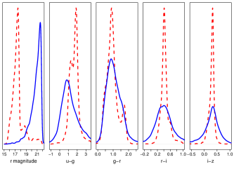
Figure 1: Estimated distributions of $r$-band model magnitudes and $ugriz$ colours for labeled (i.e. spectroscopic; red dashed lines) and unlabeled (i.e. photometric; blue solid lines) galaxies, primarily observed by the Sloan Digital Sky Survey (see Section 7). These distributions indicate the bias for selecting brighter galaxies for spectroscopic follow-up observations, which induces a covariate shift that is here manifested as mismatches in the distributions of colours between labeled and unlabeled data.

An issue that arises when constructing $\widehat{f}(z|\boldsymbol{x})$ via empirical techniques is that of selection bias. A standard assumption in statistics and machine learning is that labeled and unlabeled data are sampled from similar distributions, which we denote $\mathbb{P}_{L}$ and $\mathbb{P}_{U}$ respectively. However, as Figure 1 demonstrates, these two distributions can differ greatly for sky surveys that mix spectroscopy and photometry; brighter galaxies are more likely to be selected for follow-up spectroscopic observation. To model how selection bias affects learning methods, one needs to invoke additional assumptions about the relationship between $\mathbb{P}_{L}$ and $\mathbb{P}_{U}$ (e.g. Gretton et al. 2008, Moreno-Torres et al. 2012). In this work, we assume that the probability that a galaxy is labeled with a spectroscopic redshift depends only upon $\boldsymbol{x}$ (in accord with Lima et al. 2008 and Sheldon et al. 2012); i.e.

$$P(S=1|\boldsymbol{x},z)=P(S=1|\boldsymbol{x})\,$$ (1)

where the random variable $S$ equals $1$ if a datum is labeled and $0$ otherwise. This assumption implies covariate shift, defined as

$$f_{L}(\boldsymbol{x})\neq f_{U}(\boldsymbol{x}),\ \ f_{L}(z|\boldsymbol{x})=f_{U}(z|\boldsymbol{x})\,,$$ (2)

and thus is, as shown below, critical for establishing the risk function estimators that ultimately allow us to estimate conditional density estimates $\widehat{f}(z|\boldsymbol{x})$. Following the discussion of Section 2.3 of Budavári (2009), we point out that assuming $P(S=1|\boldsymbol{x},z)=P(S=1|\boldsymbol{x})$ can be problematic, for instance when only colours are used in analyses in which the training data are selected in limited magnitude regimes. In this work we apply our framework to galaxies at SDSS depth using colours only; for optimal performance, one should incorporate those covariates that act in concert with $z$ to affect selection, e.g., morphology, size, surface brightness, environment, etc. Nothing in the current framework prevents the incorporation of these covariates.

At first glance, it may seem that covariate shift would not pose a problem for density estimation; if $f(z|\boldsymbol{x})$ is the same for both labeled and unlabeled samples, one might infer that a good estimator of $f(z|\boldsymbol{x})$ based on labeled data would also perform well for unlabeled data. However, this is generally untrue. The estimation of $f(z|\boldsymbol{x})$ depends on the marginal distribution $f(\boldsymbol{x})$, so an estimator that performs well with respect to $f_{L}(\boldsymbol{x})$ may not perform well with respect to $f_{U}(\boldsymbol{x})$.

We can mitigate selection bias by preprocessing the labeled data so as to ensure that sufficient labeled data lay where the unlabeled data lay. This allows us to compute expected values with respect to the distribution $\mathbb{P}_{U}$ using $\mathbb{P}_{L}$, similar to the idea of importance sampling in Monte Carlo methods. Carrying this mitigation out in practice involves two steps: first, we estimate importance weights as a function of the predictors $\boldsymbol{x}$:

$$\beta(\boldsymbol{x})=f_{U}(\boldsymbol{x})/f_{L}(\boldsymbol{x})\,;$$ (3)

and second, we utilize these weights when estimating conditional densities $f(z|\boldsymbol{x})$. There are a myriad of estimators both for importance weighting and for conditional density estimation (see e.g. Izbicki, Lee & Schafer 2014, Izbicki & Lee 2015); what we provide here are rigorous procedures for tuning their parameters and for choosing among them. We note here that our overall procedure can be qualitatively summarized by the following dictum: one needs good estimates of importance weights at labeled data points in order to achieve good conditional density estimates at unlabeled data points. (One can observe how this dictum plays out mathematically in equation 11 below: note how the importance weight estimates at labeled points enter into it, in the second term, whereas the importance weight estimates at unlabeled points do not enter into it at all.)

3 Importance Weight Estimation

A naive method for computing importance weights $\beta(\boldsymbol{x})$ would involve estimating $f_{U}$ and $f_{L}$ separately and computing the ratio of these densities, but this approach can enhance errors in individual density estimates, particularly in regimes where $f_{L}\rightarrow 0$ (Sugiyama et al., 2008). Many authors have thus proposed direct estimators of the ratio $\beta(\boldsymbol{x})$ (e.g. Sugiyama et al. 2008, Lima et al. 2008, Kanamori, Hido & Sugiyama 2009, Kanamori, Suzuki & Sugiyama 2012, Loog 2012, Izbicki, Lee & Schafer 2014, Kremer et al. 2015). As an example, the estimator of Lima et al. (2008) and Kremer et al. (2015) is

$$\widehat{\beta}(\boldsymbol{x})=\frac{1}{k}\frac{n_{L}}{n_{U}}\sum_{i=1}^{n_{U}}\mathbb{I}\left(\boldsymbol{x}_{i}^{U}\in V_{k}^{L}\right)\,,$$ (4)

where $V_{k}^{L}$ is the region of covariate space containing points that are closer to $\boldsymbol{x}$ then its $k^{\rm th}$ nearest labeled neighbor, and $\mathbb{I}(\cdot)$ is the indicator function.

To choose between importance weight estimators, one needs first to optimally tune the parameters of each using the training and validation data (model selection), and then assess their performance using the test data (model assessment). We determine optimal values of tuning parameters by minimizing a risk function (equation 5 below). Generating estimates $\widehat{\beta}(\boldsymbol{x})$ (and by extension $\widehat{f}(z|\boldsymbol{x})$, below) implicitly requires smoothing the observed data, with the smoothing bandwidth set such that estimator bias and variance are optimally balanced. (See e.g. Wasserman 2006.) For instance, too much smoothing (e.g. adopting a value of $k$ that is too large in nearest-neighbor-based methods) yields estimates with low variance and high bias, i.e. when applied to independent datasets sampled from the same distribution, the estimates will all look similar (i.e. will have low variance) but will be offset from the truth (i.e. will have high bias). Too little smoothing (e.g. $k$ too small) conversely yields high-variance and low-bias estimates that overfit the training data.

Algorithm 1 Conditional Density Estimation for Photometric Redshifts

Input: Pools of labeled (i.e. spectroscopic) and unlabeled (i.e. photometric-only) data, which we denote $L$ and $U$.

• Randomly sample $n_{L}$ data from $L$ and $n_{U}$ data from $U$. (Here, $n_{L}=n_{U}=15000$.)

• Given number of nearest labeled neighbors $k$ and minimum number of unlabeled data in neighborhood $u$, repopulate the labeled sample so as to increase the effective sample size, i.e., to decrease the number of labeled data with estimated importance weight zero. Such repopulation will result in photometric covariates distributions that more closely approximates that of the unlabeled sample. (See equation 4 and Algorithm 2.)

• Split $L$ and $U$ into training, validation, and test datasets. (Here, $n_{\rm train}=7000$, $n_{\rm val}=3000$, and $n_{\rm test}=5000$ for both samples.)

• Apply training and validation data to generate importance weight esimates $\widehat{\beta}(\boldsymbol{x})$ (via equation 4), tuning the estimator so as to minimize the estimated risk given in equation 7.

• Apply importance weights $\widehat{\beta}(\boldsymbol{x})$ to the estimation of conditional densities $\widehat{f}(z|\boldsymbol{x})$ (e.g. equation 8), tuning the estimator so as to minimize the risk function given in equation 11. (Here we apply the conditional density estimators dubbed NN-CS, kerNN-CS, Series-CS, and Combined by Izbicki, Lee & Freeman 2016, where CS stands for “covariate shift" and Combined stands for the combination of the kerNN-CS and Series-CS estimators. See Section 5 for details on combining estimator output.)

• Use the test data to compute the estimated risk for each conditional density estimator (equation 11). Choose the estimator with the minimum risk.

Output: Estimated conditional densities $\{\widehat{f}(z|\boldsymbol{x}_{1}^{L}),\ldots,\widehat{f}(z|\boldsymbol{x}_{n_{L}}^{L})\}$ and $\{\widehat{f}(z|\boldsymbol{x}_{1}^{U}),\ldots,\widehat{f}(z|\boldsymbol{x}_{n_{U}}^{U})\}$.

When estimating importance weights, we apply the risk function (Izbicki, Lee & Schafer, 2014; Kremer et al., 2015)

$$R(\widehat{\beta},\beta):=\int\left(\widehat{\beta}(\boldsymbol{x})-\beta(\boldsymbol{x})\right)^{2}dP_{L}(\boldsymbol{x})$$

$$=\int\widehat{\beta}^{2}(\boldsymbol{x})dP_{L}(\boldsymbol{x})-2\int\widehat{\beta}(\boldsymbol{x})\beta(\boldsymbol{x})dP_{L}(\boldsymbol{x})+\int\beta^{2}(\boldsymbol{x})dP_{L}(\boldsymbol{x})$$

$$=\int\widehat{\beta}^{2}(\boldsymbol{x})dP_{L}(\boldsymbol{x})-2\int\widehat{\beta}(\boldsymbol{x})dP_{U}(\boldsymbol{x})+C(\beta)\,,$$ (5)

where $dP_{U}(\boldsymbol{x})=\beta(\boldsymbol{x})dP_{L}(\boldsymbol{x})$ and $C(\beta)$ is a term that does not depend on the estimate $\widehat{\beta}$. (We note that here the calculation of risk is with respect to the labeled dataset distribution $\mathbb{P}_{L}$; this is in accord with the dictum stated above that we need good estimates of importance weights for the labeled data in order to achieve good estimates of conditional densities for the unlabeled data. See equation 11 below.) While we utilize an $L^{2}$-loss function above in (5) and below in (9), one could in principle substitute other functions based on F-divergences, log-densities, or notions of $L^{1}$ loss. However, functions based on F-divergences and log-densities are overly sensitive to distribution tails and are generally not appropriate for density estimation (see, e.g. Hall 1987 and Wasserman 2006), while estimating a risk based on $L^{1}$ loss requires knowledge of the true $f(z|\boldsymbol{x})$. Since in model selection and assessment we can ignore $C(\beta)$, we rewrite the above as

$$J(\widehat{\beta}) =\int\widehat{\beta}^{2}(\boldsymbol{x})dP_{L}(\boldsymbol{x})-2\int\widehat{\beta}(\boldsymbol{x})dP_{U}(\boldsymbol{x})\,,$$ (6)

which we estimate as

$$\widehat{J}(\widehat{\beta})=\frac{1}{\widetilde{n}_{L}}\sum_{k=1}^{\widetilde{n}_{L}}\widehat{\beta}^{2}\left(\boldsymbol{\widetilde{x}}_{k}^{L}\right)-\frac{2}{\widetilde{n}_{U}}\sum_{k=1}^{\widetilde{n}_{U}}\widehat{\beta}\left(\boldsymbol{\widetilde{x}}_{k}^{U}\right)\,,$$ (7)

where the tildes indicate that the risk is evaluated using either validation data (during model selection) or test data (during model assessment). (Here we use $J$ to represent a risk function in which the constant term $C(\beta)$ is ignored.) Among multiple estimators of $\widehat{\beta}(\boldsymbol{x})$, we choose the one that yields the smallest value of $\widehat{R}$ when applied to test data.

4 Conditional Density Estimation

Given an estimate $\widehat{\beta}(\boldsymbol{x})$ of the importance weight, the ratio of densities of the unlabeled and labeled data at the point $\boldsymbol{x}$, our next step is to compute estimates of the conditional density $\widehat{f}(z|\boldsymbol{x})$. Conditional density estimators include those of Cunha et al. (2009) and Izbicki & Lee (2015); see e.g. Izbicki, Lee & Freeman (2016) for more details. To build intuition here, we write down the estimator of Cunha et al. (2009), as it is particularly simple:

$$\widehat{f}(z|\boldsymbol{x})\propto\sum_{i\in\mathcal{N}_{N}(\boldsymbol{x})}\widehat{\beta}\left(\boldsymbol{x}^{L}_{i}\right)\mathbb{I}\left(z^{L}_{i}\in b(z)\right)\,,$$ (8)

where $\mathcal{N}_{N}(\boldsymbol{x})$ denotes the $N$ neighbors nearest to $\boldsymbol{x}$ among labeled data, and $b(z)$ denotes the a priori defined bin to which $z$ belongs. This estimator (up)down-weights labeled data in regions where $f_{U}(\boldsymbol{x})$ is (larger) smaller than $f_{L}(\boldsymbol{x})$.

In a selection bias setting where $\mathbb{P}_{L}\neq\mathbb{P}_{U}$, the goal of conditional density estimation is to minimize

$$R(\widehat{f},f):=\iint\left(\widehat{f}(z|\boldsymbol{x})-f(z|\boldsymbol{x})\right)^{2}dP_{U}(\boldsymbol{x})dz\,,$$ (9)

i.e. the risk with respect to the unlabeled data. Under the covariate shift assumption $f_{U}(z|\boldsymbol{x})=f_{L}(z|\boldsymbol{x})$, one can rewrite the modified risk (9) up to a constant as

$$R(\widehat{f},f)=\iint\widehat{f}^{2}(z|\boldsymbol{x})dP_{U}(\boldsymbol{x})dz$$

$$-2\iint\widehat{f}(z|\boldsymbol{x})f(z|\boldsymbol{x})dP_{U}(\boldsymbol{x})dz+\iint f^{2}(z|\boldsymbol{x})dP_{U}(\boldsymbol{x})dz$$

$$=\iint\widehat{f}^{2}(z|\boldsymbol{x})dP_{U}(\boldsymbol{x})dz-2\iint\widehat{f}(z|\boldsymbol{x})\beta(\boldsymbol{x})dP_{L}(z,\boldsymbol{x})+C(f)\,,$$ (10)

where the second equality follows from $f_{U}(z|\boldsymbol{x})dP_{U}(\boldsymbol{x})dz=f_{L}(z|\boldsymbol{x})\beta(\boldsymbol{x})dP_{L}(\boldsymbol{x})dz=\beta(\boldsymbol{x})dP_{L}(z,\boldsymbol{x})$. Again, this risk depends upon unknown quantities; we ignore $C(f)$ and estimate the other terms via the equation

$$\widehat{J}(\widehat{f})=\frac{1}{\widetilde{n}_{U}}\sum_{k=1}^{\widetilde{n}_{U}}\left[\int\widehat{f}^{2}\left(z|\widetilde{\boldsymbol{x}}_{k}^{U}\right)dz\right]-\frac{2}{\widetilde{n}_{L}}\sum_{k=1}^{\widetilde{n}_{L}}\widehat{f}\left(\widetilde{z}^{L}_{k}|\widetilde{\boldsymbol{x}}^{L}_{k}\right)\widehat{\beta}\left(\widetilde{\boldsymbol{x}}^{L}_{k}\right)\,,$$ (11)

where again the tildes indicate use of validation data in model selection and test data in model assessment.

5 Combining Estimators

Typical photometric redshift estimation methods utilize one method for computing $\widehat{z}|\boldsymbol{x}$ or ${\widehat{f}}(z|\boldsymbol{x})$. However, one can improve upon the prediction performances of individual estimators by combining them. Suppose that $\widehat{f}_{1}(z|\boldsymbol{x}),\ldots,\widehat{f}_{p}(z|\boldsymbol{x})$ are $p$ separate estimators of $f(z|\boldsymbol{x})$. We define the weighted average to be

$$\widehat{f}^{{\boldsymbol{\alpha}}}(z|\boldsymbol{x})=\sum_{k=1}^{p}\alpha_{k}\widehat{f}_{k}(z|\boldsymbol{x}),$$ (12)

where the weights minimize the empirical risk $\widehat{R}(\widehat{f}^{{\boldsymbol{\alpha}}})$ under the constraints $\alpha_{i}\geq 0$ and $\sum_{i=1}^{p}\alpha_{i}=1$. One can determine the solution ${\boldsymbol{\alpha}}=\left[\alpha_{i}\right]_{i=1}^{p}$ by solving a standard quadratic programming problem:

$$\underset{{\boldsymbol{\alpha}}:\alpha_{i}\geq 0,\sum_{i=1}^{p}\alpha_{i}=1}{\arg\min}{\boldsymbol{\alpha}}^{\prime}\mathbb{B}{\boldsymbol{\alpha}}-2{\boldsymbol{\alpha}}^{\prime}b\,,$$ (13)

where $\mathbb{B}$ is the $p\times p$ matrix

$$\left[\frac{1}{\widetilde{n}_{U}}\sum_{k=1}^{\widetilde{n}_{U}}\int\widehat{f}_{i}(z|\widetilde{\boldsymbol{x}}_{k}^{U})\widehat{f}_{j}(z|\widetilde{\boldsymbol{x}}_{k}^{U})dz\right]_{i,j=1}^{p}$$ (14)

and $b$ is the vector

$$\left[\frac{1}{\widetilde{n}_{L}}\sum_{k=1}^{\widetilde{n}_{L}}\widehat{f}_{i}(\widetilde{z}^{L}_{k}|\widetilde{\boldsymbol{x}}^{L}_{k})\widehat{\beta}(\widetilde{\boldsymbol{x}}^{L}_{k})\right]_{i=1}^{p}\,;$$ (15)

the tildes here indicate use of the validation data.

6 Diagnostic Tests for Estimators

Risk estimates, such as those given in equations 7 and 11, allow us to tune estimators and to choose between estimators, but they do not ultimately convey how well the estimator performs in an absolute sense. Below we describe diagnostic tests that one can use to more closely assess the quality of different models. Similar tests can be found in the time series literature (see, e.g., Corradi & Swanson 2006).

6.1 Assessing uniformity using empirical CDFs

Let $\widehat{F}(z|\boldsymbol{x}_{i})$ denote the estimated conditional cumulative distribution function, i.e., let

$$U_{i}=\widehat{F}(z_{i}|\boldsymbol{x}_{i})=\int_{0}^{z_{i}}\widehat{f}(y|\boldsymbol{x}_{i})dy\,.$$ (16)

If the chosen estimator performs well, then the empirical cumulative distribution function (CDF) of the values $U_{1},\ldots,U_{n}$ will be consistent with the CDF of the uniform distribution. We can test this hypothesis via, e.g., the Cramér-von Mises, Anderson-Darling, and Kolmogorov-Smirnoff tests. If the $p$-value output by the test is $>0.05$, then we fail to reject the null hypothesis that the data $U_{1},\ldots,U_{n_{\widehat{\beta}_{o}}}$ are sampled from a uniform distribution.

6.2 Assessing uniformity using quantiles

We can use the values $U_{1},\ldots,U_{n}$ defined above to build a quantile-quantile (or QQ) plot, by determining the number of data in bins of width $\Delta U$. Let $J$ be the number of bins, each of which has midpoint $c_{j}$ and the fraction of data $\widehat{c}_{j}$. The QQ plot is that of the values $\widehat{c}_{j}$ against $c_{j}$; if the chosen estimators perform well, the points in this plot will approximately lie on the line $\widehat{c}=c$. We assess consistency with uniformity via the chi-square goodness of fit (GoF) test, which utilizes the chi-square statistic

$$\chi_{\rm obs}^{2}=\sum_{j=1}^{J}\frac{(n\widehat{c}_{j}-n/J)^{2}}{n/J}\,.$$ (17)

We conclude that the difference data are consistent with constancy if the $p$ value, the fraction of the time that a value of $\chi^{2}$ would be observed that is greater than $\chi_{\rm obs}^{2}$ if the null hypothesis of constancy is true, is $>0.05$. Note that the off-the-shelf GoF test, which allows one to compute the $p$ value by taking the tail integral of an appropriate chi-square distribution, requires that the number of expected counts in each bin be $\gtrsim$ 5. When that condition is violated, one should use simulations to estimate $p$ values.

6.3 Assessing uniformity in interval coverage

For every $\alpha_{j}$ in a grid of values on $[0,1]$ of length $J$, and for every observation $i$ in the labeled test sample, we determine the smallest interval $A_{ij}=[z_{i}^{\rm lo},z_{i}^{\rm hi}]$ such that

$$\int_{A_{ij}}\widehat{f}(z|\boldsymbol{x}_{i})dz=\alpha_{j}\,.$$ (18)

Then, for every $\alpha_{j}$, we determine the proportion of redshifts lie within $A_{ij}$, i.e. we compute

$$\widehat{\alpha}_{j}=\sum_{i\in S}\mathbb{I}(z_{i}^{L}\in A_{ij})\,.$$ (19)

If the chosen estimators perform well, then $\widehat{\alpha}\approx\alpha$. We plot the values of $\widehat{\alpha}$ against corresponding values of $\alpha$ and assess how close the plotted points are to the line $\widehat{\alpha}=\alpha$; we can test for consistency with that line using the chi-square GoF test, as described above.

Note that the construction of coverage plots is also proposed by Wittman, Bhaskar & Tobin (2016), who conclude that the $\widehat{f}(z|\boldsymbol{x})$ produced by the template-based BPZ and EAZY codes are consistently too narrow and approximately correct, respectively.

7 Application to SDSS Data

7.1 Data

To demonstrate the efficacy of our conditional density estimation method, we apply it to $\approx$10⁶ galaxies that are mostly from Data Release 8 of the Sloan Digital Sky Survey (Aihara et al., 2011).

To build our unlabeled (i.e. photometric) dataset, we initially extract model magnitudes for 540,235 objects in the sky patch RA $\in$ [168^∘,192^∘] and $\delta\in[-1.5^{\circ},1.5^{\circ}]$. After filtering these data in the manner of Sheldon et al. (2012), namely limiting our selection to those data whose $ugriz$ magnitudes were all between 15 and 29, and then further limiting ourselves to data for which

$$$u < 21$~{}~{}{\rm or}~{}~{}$g < 22$~{}~{}{\rm or}~{}~{}$r < 22$~{}~{}{\rm or}~{}~{}$i < 20.5$~{}~{}{\rm or}~{}~{}$z < 20.1$\,,$$

we obtain a sample of 538,974 objects.

We use the labeled (i.e. spectroscopic) dataset of Sheldon et al. (2012) (E. Sheldon, private communication). This dataset includes 435,875 objects from SDSS DR8 and 31,835 objects from eight other sources, or 467,710 objects in all. As noted by Sheldon et al., this dataset contains a small number of stars. We remove these by excluding all data with spectroscopic redshift $z_{s}=0$; after this, we are left with 465,790 objects.

The steps of our analysis are given in Algorithms 1 and 2. As noted in Section 2, the labeled and unlabeled data that we analyse are samples from the larger pools of available data described immediately above. (In this work we set $n_{L}=n_{U}=15{,}000$.) This is for computational efficiency, both from a standpoint of time and memory; for instance, if we utilize matrices for storing distances between data points, we are currently limited to samples of size $\sim$ 10⁴ when utilizing typical desktop computers.

Algorithm 2 Preprocessing Labeled (i.e. Spectroscopic) Data

Input: Number of labeled and unlabeled data, $n_{L}$ and $n_{U}$.

        Labeled dataset $L=\{\boldsymbol{x}_{1}^{L},\ldots,\boldsymbol{x}_{n_{L}}^{L}\}$ and unlabeled dataset $U=\{\boldsymbol{x}_{1}^{U},\ldots,\boldsymbol{x}_{n_{U}}^{U}\}$.

        Number of nearest labeled neighbors, $k$.

        Minimum number of unlabeled data required for selection of new labeled datum, $u$.

• Randomly permute all labeled data indices (i.e. those from the larger pool of all available labeled data).

• Loop over the permuted set of indices $i_{p}$:

• estimate $\widehat{\beta}(\boldsymbol{x}_{i_{p}})$ within the volume containing the $k$ nearest neighbors among $L$ (via e.g. equation 4)

• if $\widehat{\beta}(\boldsymbol{x}_{i_{p}})\geq u/k$, accept $\boldsymbol{x}_{i_{p}}$ as a new labeled datum

• if the number of new labeled data equals $n_{L}$, terminate loop.

Output: New labeled dataset $\{\boldsymbol{x}_{1}^{L},\ldots,\boldsymbol{x}_{n_{L}}^{L}\}$.

          The importance weights for these data are re-estimated and are applied to conditional density estimation (e.g. equation 8, and equation 11).

7.2 Data preprocessing: construction of the labeled sample

As shown in equation 8, the estimation of conditional densities is partially a function of $\widehat{\beta}(\boldsymbol{x}^{L})$, so there is a distinction to be drawn between the stated labeled sample size (e.g. $n_{L}$ = 15000, drawn from a pool of size 465,790) and the effective size (the number of data that contribute to estimation, i.e. the number for which $\widehat{\beta}(\boldsymbol{x}^{L})>0$). Thus one important step of our method involves preprocessing the labeled data to increase their effective size.

The preprocessing of the labeled data requires the specification of a threshold importance weight $\widehat{\beta}_{\rm thr}$. Given $n_{L}$ and $n_{U}$ labeled and unlabeled data, respectively, and having specified a minimum number of unlabeled data $u$ that would have to lie closer to a random labeled point $\boldsymbol{x}^{L}$ (drawn from the larger pool) than the $k^{\rm th}$ nearest labeled neighbor to that point, we keep $\boldsymbol{x}^{L}$ as part of our new labeled dataset if

$$\widehat{\beta}(\boldsymbol{x}^{L})\geq\widehat{\beta}_{\rm thr}=\frac{u}{k}\,.$$ (20)

The value $\widehat{\beta}_{\rm thr}$ is not tunable, per se, as different thresholds yield different labeled datasets, leading to estimated risks that are not directly comparable. One might conjecture that larger values of $\widehat{\beta}_{\rm thr}$ are better, in that the distribution of the labeled data will more closely resemble that of the unlabeled data (see Figures 1 and 2). However, as we demonstrate below, our results are not highly sensitive to the choice of $\widehat{\beta}_{\rm thr}$, so long as $\widehat{\beta}_{\rm thr}>0$.

Once preprocessing is complete, we repeat the estimation of the importance weights $\widehat{\beta}(\boldsymbol{x}^{L})$ and apply these values when estimating conditional densities (e.g. equation 8, and equation 11).

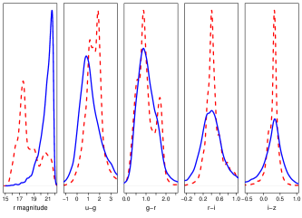
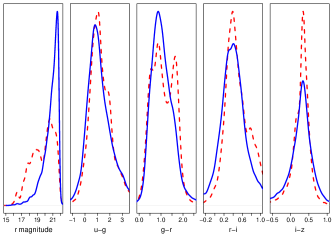
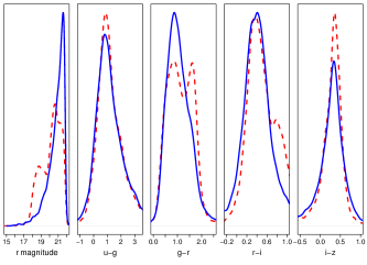
Figure 2: Same as Figure 1, except that here we construct the labeled data with the preprocessing scheme outlined in Algorithm 2 so as to increase the effective sample size (i.e. the number of labeled data with non-zero importance weights). The panels exhibit preprocessing with $\widehat{\beta}_{\rm thr}=0.1,0.2$ and $0.3$, respectively from top to bottom (see equation 20). (For larger values of $\widehat{\beta}_{\rm thr}$, we cannot fully populate a labeled subsample of size $n_{L}=15000$ from the pool of labeled data at our disposal.) In all three cases, the distributions for the labeled data (red dashed lines) more closely resembles those for the unlabeled data (blue solid lines), relative to the labeled distributions exhibited in Figure 1. Subsequent to preprocessing we re-estimate the importance weights $\widehat{\beta}(\boldsymbol{x}^{L})$ and apply these values to the estimation of conditional densities (e.g. equation 8, and equation 11).

7.3 Results

Once we generate our new labeled dataset, we split the labeled and unlabeled data into training ($n_{\rm train}=7000$), validation ($n_{\rm valid}=3000$), and test ($n_{\rm test}=5000$) sets. We forego model assessment for importance weight estimators in this work; Izbicki, Lee & Freeman (2016) demonstrate that the estimator given in equation 4 consistently performs better than five other competing methods over a number of different levels of covariate shift. We apply equations 4 and 7 to the training and validation data to determine the optimal number of nearest neighbors $k$ and importance weights $\widehat{\beta}(\boldsymbol{x}^{L})$ given $k$. We then apply these importance weights and the estimated risk in equation 11 to the training and validation data within the context of three CDE estimators detailed in Izbicki, Lee & Freeman (2016): NN-CS, the estimator of Cunha et al. (2009); kerNN-CS, a kernelized variation of NN-CS; and Series-CS, the spectral series estimator of Izbicki & Lee (2015). In Figure 3 we demonstrate the importance of preprocessing to generate the labeled dataset: without it, the construction of conditional density estimates for the unlabeled data would be effectively limited to the regime $\widehat{\beta}(\boldsymbol{x}^{U})\lesssim 0.5$. The fraction of unlabeled test set data with $\widehat{\beta}(\boldsymbol{x}^{U})\leq 0.5$ is approximately 7.5%; in contrast, the fraction for $\widehat{\beta}(\boldsymbol{x}^{U})\leq 3$ is 88.5%. In Figure 4 we demonstrate that for our particular SDSS data, the kerNN-CS estimator on average outperforms the other two. (Note that the risk can be negative because we ignore the positive additive constant $C(f)$; see equation 10.) We use the method outlined in Section 5 to optimally combine the conditional density estimates from kerNN-CS and Series-CS and we determine that combining these estimators, on average, indeed yields better estimates of the conditional densities $\widehat{f}(z|\boldsymbol{x})$.

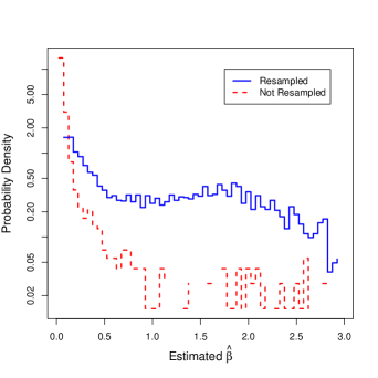
Figure 3: Estimated probability density functions for $\widehat{\beta}(\boldsymbol{x}^{L})$ before (red dashed line) and after (blue solid line) application of the labeled data preprocessing scheme described in Section 7.2 and Algorithm 2. Without preprocessing, there are effectively no data with which to learn a statistical model linking the covariates and redshift in the regime $\widehat{\beta}(\boldsymbol{x}^{L})\gtrsim 0.5$, a regime that contains $>$ 90% of the unlabeled data.

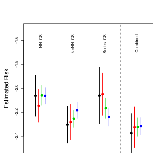
Figure 4: Estimated risk (and standard errors) resulting from the application of the NN-CS, kerNN-CS and Series-CS conditional density estimators, and a combination of the latter two (see Section 5). The four points in each group represent different values for the importance weight threshold $\widehat{\beta}_{\rm thr}$ in our scheme for preprocessing labeled data; from left to right, $\widehat{\beta}_{\rm thr}=0.0,0.1,0.2,$ and $0.3$ (black, red, green, and blue respectively). The estimated risks for each $\widehat{\beta}_{\rm thr}$ were adjusted to have mean $-$2.2. In all four cases, we observe that combining the kerNN-CS and Series-CS estimators leads to better conditional density estimates than either yield themselves.

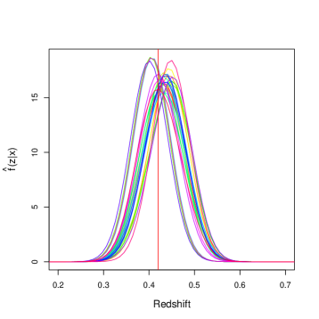
Figure 5: Twenty-five estimates of $\widehat{f}(z|\boldsymbol{x})$ made for a single labeled test-set galaxy via bootstrapping of the labeled training dataset. The solid red vertical line indicates the true redshift. As described in the text, we make a preliminary assessment of the noise properties of $\widehat{f}(z|\boldsymbol{x})$ by computing the true redshift quantile for each curve (i.e. the integral of the curve between zero and the true redshift), computing the sample standard deviation of these quantiles, and determining the overall mean standard deviation. Here, the standard deviation of the quantiles is $\approx$ 0.13; on average the standard deviation is $\approx$ 0.06.

We make a preliminary assessment of the noise properties of the estimates $\widehat{f}(z|\boldsymbol{x})$ as follows. We create $n$ bootstrap samples of the labeled training data and use them to generate $n$ $\widehat{f}(z|\boldsymbol{x})$ curves for each labeled test datum. (See Figure 5.) Then we compute the quantile of the true redshift given each curve, so that for each labeled test datum we have $n$ quantile values. We use the mean of the standard deviations of each set of quantile values as a metric of uncertainty. For our particular SDSS data, we determine this mean uncertainty to be $\approx$ 0.065. We will examine the noise properties of the estimates $\widehat{f}(z|\boldsymbol{x})$ at greater depth in a future work.

In Figure 6 we demonstrate the tradeoff that is inherent when mitigating covariate shift, via the incorporation of importance weights into estimation, using QQ plots. If we do not mitigate covariate shift, we achieve good conditional density estimates within those portions of covariate space in which $\widehat{\beta}(\boldsymbol{x}^{L})\lesssim 0.5$ (orange dashed-dotted line); however, $\lesssim$ 8% of the unlabeled data reside within these portions. Mitigation of covariate shift leads to a worsening of the CDEs within these portions of covariate space (black dashed line), but allows one to make good estimates throughout the remaining space (blue solid line). In Figures 7, 8 and 9 we show the results of applying hypothesis tests based on QQ plots (Section 6.2), coverage plots (Section 6.3) and the assumption of uniformity (Section 6.1). In the first two figures we show the results of using the GoF test to determine the consistency of expected and observed quantiles at each unique value of $\widehat{\beta}(\boldsymbol{x}^{L})$, in the manner outlined in Section 6. These results are generated using the labeled test set data, assuming a preprocessing threshold $\widehat{\beta}_{\rm thr}=0.3$. (The optimal number of nearest neighbors given this threshold is 20, hence the unique values of $\widehat{\beta}(\boldsymbol{x}^{L})$ are 0, 0.05, 0.1, etc.) In the middle and bottom panels, we observe that for $\widehat{\beta}(\boldsymbol{x}^{L})\lesssim 0.3$, the chi-square values are much larger, and the $p$ values much smaller, than what we would expect if $\widehat{c}=c$: we do not achieve good behavior in this regime. (This is consistent with the behavior of the QQ plots shown in Figure 6.) For $\widehat{\beta}(\boldsymbol{x}^{L})\gtrsim 0.3$, on the other hand, the $p$ values are generally $>0.05$. We thus conclude that our method generates useful conditional density estimates in the regime $\widehat{\beta}(\boldsymbol{x}^{L})\gtrsim 0.3$. (We note that we come to similar conclusions if we use the preprocessing thresholds $\widehat{\beta}_{\rm thr}=0.1$ or $0.2$ instead.)

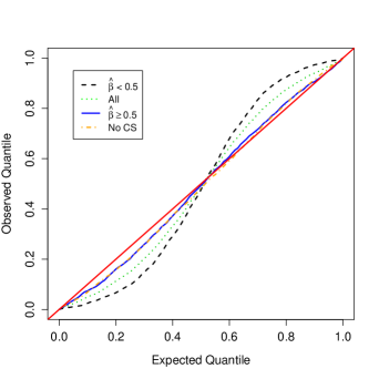
Figure 6: Quantile-quantile results for all labeled test data (green dotted line), labeled test data for which $\widehat{\beta}(\boldsymbol{x}^{L})<0.5$ and $\geq 0.5$ (black dashed and blue solid lines respectively), and labeled test data for the case where we do not mitigate covariate shift by incorporating importance weights into estimation (orange dashed-dotted line, largely following the blue solid line), which effectively limits modeling to the regime $\widehat{\beta}(\boldsymbol{x}^{L})\lesssim 0.5$ (see Figure 3). This plot demonstrates that mitigating covariate shift leads to worse conditional density estimates in the portion of covariate space where $\widehat{\beta}(\boldsymbol{x}^{L})\lesssim 0.5$ and where $\lesssim$ 8% of the unlabeled data are located (orange line vs. black line), but yields good estimates throughout the remaining covariate space (blue line vs. orange line).

Figure 9 shows the results of applying the Cramér-von Mises, Anderson-Darling, and Kolmogorov-Smirnov tests (from top to bottom, respectively) to the data $U$ generated from the CDFs of the conditional density estimates $\widehat{f}(z|\boldsymbol{x})$ of the labeled test set data, again assuming $\widehat{\beta}_{\rm thr}=0.3$. We observe similar behavior for the $p$ values here as observed in Figure 7, with two differences: (1) the $p$ values are generally above 0.05 for $\widehat{\beta}(\boldsymbol{x}^{L})\gtrsim 0.5$ as opposed to 0.3, and (2) there are more numerous deviations from uniformity in the regime $\widehat{\beta}(\boldsymbol{x}^{L})\gtrsim 0.5$ than seen in the bottom panel of Figure 7, particularly in the case of the AD test (middle panel, Figure 9).

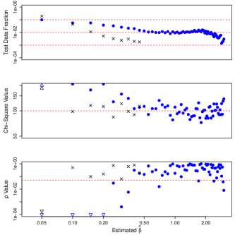
Figure 7: Results of testing whether the observed quantile value differences ($\widehat{c}_{1}-\widehat{c}_{0},\ldots,\widehat{c}_{B}-\widehat{c}_{B-1}$) are constant across quantile bins, using the labeled test set data at each unique value of $\widehat{\beta}(\boldsymbol{x}^{L})$. Our estimates of $\widehat{f}(z|\boldsymbol{x})$ are generated via the Combined estimator. In all panels, the blue dots/black crosses represent results generated with/without covariate shift mitigation (i.e. with/without the incorporation of importance weights into estimation), with the blue/black triangles specifying data points that fall outside the plot panels. (There are insufficient data above $\widehat{\beta}(\boldsymbol{x}^{L})\geq 0.5$ to generate results without mitigating covariate shift.) The top panel shows the fraction of data for each unique value, with the dashed red lines indicating 0.1%, 1%, and 10% respectively. The middle panel shows the chi-square statistic resulting from each test, with the red dashed line indicating the number of bins ($B=100$), the value to which chi square should converge if our estimator performs well in regions of covariate space with appreciable densities of unlabeled data. The bottom panel shows the $p$ value, estimated via simulation since the usual assumption of the chi-square goodness of fit test that there are at least five expected counts in each bin is usually violated; the red dashed line indicates $p=0.05$, with points above that line indicating that the observed quantile value differences are consistent with constancy across quantile bins. The middle and bottom panels demonstrate that our method achieves desired quantile-quantile behavior at $\widehat{\beta}(\boldsymbol{x}^{L})\gtrsim 0.3$, while also demonstrating the importance of assuming covariate shift with these data: without this assumption, we can only generate reasonable predictions for unlabeled data in the regime $\widehat{\beta}(\boldsymbol{x}^{L})\lesssim 0.5$. We assume $\widehat{\beta}_{\rm thr}=0.3$; analogous plots for $\widehat{\beta}_{\rm thr}=0.1$ and $0.2$, not shown, indicate similar results.

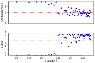
Figure 8: Same as Figure 7, except instead of quantile-quantile behavior we examine the differences between observed and expected coverage as a function of $\widehat{\beta}(\boldsymbol{x}^{L})$, and only for the case where we mitigate covariate shift. The top and bottom panels demonstrate that our method achieves good coverage for $\widehat{\beta}(\boldsymbol{x}^{L})\gtrsim 0.5$.

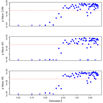
Figure 9: Results of testing whether the observed random variables $U_{i}=\widehat{F}(z_{i}|\boldsymbol{x}_{i})$ are uniformly distributed, using the labeled test set data at each unique value of $\widehat{\beta}(\boldsymbol{x}^{L})$. Our estimates of $\widehat{F}(z|\boldsymbol{x})$ are generated via the Combined estimator. The panels show $p$ values generated via the Cramér-von Mises (CvM), Anderson-Darling (AD), and Kolmogorov-Smirnov (KS) tests, from top to bottom respectively. The KS test statistic is the maximum deviation of the empirical cumulative distribution function (CDF) for $U$ from the uniform CDF, while the CvM and AD statistics are based on (unweighted and weighted) integrated distances between the empirical and uniform CDFs. These panels demonstrate that our method generally achieves good behavior with respect to uniformity at $\widehat{\beta}(\boldsymbol{x}^{L})\gtrsim 0.5$ (cf. 0.3 and 0.5 for tests based on QQ and coverage plots). This plot shows results for the preprocessing threshold $\widehat{\beta}_{\rm thr}=0.3$; analogous plots for $\widehat{\beta}_{\rm thr}=0.1$ and $0.2$, not shown, indicate similar results.

8 Summary

In this paper, we provide a principled method for generating conditional density estimates $\widehat{f}(z|\boldsymbol{x})$ (elsewhere commonly denoted $p(z)$ and dubbed the “photometric redshift PDF") that takes into account selection bias and the covariate shift that this bias induces. (See Figure 1 for an example of both: a bias towards brighter galaxies leads to shifted distributions of colours between spectroscopic and photometric data samples. See also Algorithms 1 and 2.) If not mitigated, covariate shift leads to situations where models fit to labeled (i.e. spectroscopic) data will not produce scientifically useful fits to the far more numerous unlabeled (i.e. photometric-only) data, lessening the impact of photo-z estimation within the context of precision cosmology. Here, we mitigate covariate shift by first estimating importance weights, the ratio $\beta(\boldsymbol{x})$ between the densities of unlabeled and labeled data at point $\boldsymbol{x}$ (Section 3), and then applying these weights to conditional density estimates $\widehat{f}(z|\boldsymbol{x})$ (Section 4).

In order for our two-step procedure to succeed, ultimately, we require good estimates of $\beta(\boldsymbol{x})$ at labeled data points in order for it to achieve good estimates $\widehat{f}(z|\boldsymbol{x})$ at unlabeled ones. We thus need both rigorously defined risk functions that allow us to tune the free parameters of our importance weight and conditional density estimators, and diagnostic tests that allow us to determine the quality of the estimates $\widehat{f}(z|\boldsymbol{x})$. Our method is based on the assumption that the probability that astronomers label a galaxy (i.e. determine its spectroscopic redshift) depends only on its (photometric and perhaps other) properties $\boldsymbol{x}$ and not on its true redshift, an assumption currently valid for redshifts $\lesssim$0.5. This is equivalent to assuming that the conditional densities for labeled and unlabeled data match ($f_{L}(z|\boldsymbol{x})=f_{U}(z|\boldsymbol{x})$), even if the marginal distributions differ ($f_{L}(\boldsymbol{x})\neq f_{U}(\boldsymbol{x})$), which allows us ultimately to substitute out the true unknown quantities $\beta(\boldsymbol{x})$ and $f(z|\boldsymbol{x})$ in specifications of risk functions (equations 7 and 11). These risk functions, and their estimates (equations 7 and 11), are the backbone of our method: they allow us to tune parameters in a principled manner (e.g. what is the optimal number of nearest labeled neighbors when estimating $\beta(\boldsymbol{x})$ via equation 4?), as well as choose between competing estimators (e.g. which is better: the NN-CS, kerNN-CS or Series-CS estimators of conditional density?). An important question to answer in future work is whether we can relax our central assumption and still be able to write down estimated risks that lead to useful estimates of conditional densities in higher redshift regimes.

In Section 5, we demonstrate that once we generate $p$ separate conditional density estimates $\widehat{f}_{k}(z|\boldsymbol{x})$ (e.g. via the kerNN-CS and Series-CS estimators), tuned via the estimated risk given in equation 11, we can combine them to achieve better predictions (i.e. smaller values of risk). The method we propose utilizes a weighted linear combination, with the weights determinable via quadratic programming, but this is not the only possible way to combine estimates; see, e.g., Dahlen et al. (2013), who discuss three methods for combining estimates, including one (Method 2) that adds estimates together as we do, except that while we determine optimal coefficients by minimizing estimated risk, they combine estimates so that 68.3% of the spectroscopic redshifts in their sample fall within their final 1$\sigma$ confidence intervals.

It is not sufficient to generate estimates $\widehat{f}(z|\boldsymbol{x})$ by minimizing risk; one also needs to demonstrate that the estimates are scientifically useful. There is no unique way to demonstrate the quality of conditional density estimates. In Section 6, we provide alternatives that test (1) whether estimated cumulative densities, evaluated at actual redshifts, are distributed uniformly; (2) whether observed quantiles match expectation via QQ plots and the chi-square GoF test; and (3) testing uniformity as a function of interval coverage. The jury is still out as to which of these diagnostics will play a central role in future photo-z analyses; for now, we consider it sufficient to demonstrate in any analysis that these diagnostics yield similar qualitative results.

In Section 7, we demonstrate our method using $\approx$500,000 galaxies with, and $\approx$500,000 without, spectroscopic redshifts, mostly from the Sloan Digital Sky Survey (see Sheldon et al. 2012 for details). For computational efficiency, we sample 15,000 galaxies from both pools of data. While our initial labeled sample is chosen randomly from the larger pool of labeled data, we implement a preprocessing scheme (see Algorithm 2) to generate a new labeled sample with a larger effective size, whose photometry also more closely resembles that of the unlabeled sample (see Figure 2). The preprocessing scheme requires the specification of an importance weight threshold ($\widehat{\beta}_{\rm thr}$) whose value cannot be optimized via tuning (since different thresholds yield different labeled datasets, and thus yield not-directly comparable estimated risks). We demonstrate that our results are generally insensitive to the choice of threshold within the regime $\widehat{\beta}_{\rm thr}\lesssim 0.3$. Those results include that (1) as expected, the conditional density of Combined estimator, constructed from those of the kerNN-CS and Series-CS estimators, provide the best estimates as quantified via the risk estimate in equation 11, and (2) via our diagnostic tests, we determine that our Combined estimates exhibit good behavior in the regimes $\widehat{\beta}(\boldsymbol{x})\gtrsim 0.3$, for QQ-based tests, and $\gtrsim 0.5$, for tests of coverage and cumulative densities. Our results thus demonstrate that our method achieves good, i.e. scientifically useful, conditional density estimates for unlabeled galaxies.

References

- Aihara et al. (2011) Aihara H., et al., 2011, ApJS, 193(2):29
- Ball & Brunner (2010) Ball N. M., Brunner R. J., 2010, International Journal of Modern Physics D, 19, 1049
- Benítez (2000) Benítez N., 2000, ApJ, 536, 571
- Bonnett (2015) Bonnett C., 2015, MNRAS, 449, 1043
- Brammer, von Dokkum & Coppi (2008) Brammer G., von Dokkum P., Coppi P., 2008, ApJ, 686, 1503
- Budavári (2009) Budavári T., 2009, ApJ, 695, 747
- Carliles et al. (2010) Carliles S., Budavári T., Heinis S., Priebe C., Szalay A. S., 2010, ApJ, 712, 511
- Carrasco Kind & Brunner (2013) Carrasco Kind M., Brunner R., 2013, MNRAS, 432, 1483
- Carrasco Kind & Brunner (2014) Carrasco Kind M., Brunner R., 2014, MNRAS, 438, 3409
- Collister & Lahav (2004) Collister A. A., Lahav O., 2004, PASP, 116, 345
- Corradi & Swanson (2006) Corradi V., Swanson N. R., 2006, in Elliott G., Granger C., Timmermann A., eds, Handbook of Economic Forecasting. Elsevier, Amsterdam, p. 197
- Csabai et al. (2007) Csabai I., Dobos L., Trencséni M., Herczegh G., Jósza P., Purger N., Budavári T., Szalay A. S., 2007, Astronomische Nachrichten, 328, 852
- Cunha et al. (2009) Cunha C. E., Lima M., Oyaizu H., Frieman J., Lin H., 2009, MNRAS, 396, 2379
- Dahlen et al. (2013) Dahlen T., et al., 2013, ApJ, 775, 93
- De Vicente, Sánchez & Sevilla-Noarbe (2016) De Vicente J., Sánchez E., Sevilla-Noarbe I., 2016, MNRAS, 459, 3078
- Flaugher (2005) Flaugher B., 2005, Int. J. Modern Phys. A, 20, 3121
- Gretton et al. (2008) Gretton A., Smola A., Huang J., Schmittfull M., Borgwardt K., Schölkopf B., 2008, in Quionero-Candela J., Sugiyama M., Schwaighofer A., Lawrence N. D., eds, Dataset Shift in Machine Learning. MIT Press, Cambridge
- Hall (1987) Hall P., 1987, The Annals of Statistics, 15, 1491
- Hildebrandt et al. (2010) Hildebrandt H., et al., 2010, A&A, 523, A31
- Hoyle et al. (2015) Hoyle B., Rau M. M., Bonnett C., Seitz S., Weller J., 2015, MNRAS, 450, 305
- Ivezić et al. (2008) Ivezić Ž., 2008, arXiv:0805.2366
- Izbicki, Lee & Freeman (2016) Izbicki R., Lee A., Freeman P. E., 2016, Annals of Applied Statistics, submitted (arXiv:1604.01339)
- Izbicki & Lee (2015) Izbicki R., Lee A. B., 2015, Journal of Computational and Graphical Statistics
- Izbicki, Lee & Schafer (2014) Izbicki R., Lee A., Schafer, C. M., 2014, Journal of Machine Learning Research W&CP (AISTATS track), 33
- James et al. (2014) James G., Witten D., Hastie T., Tibshirani, R., 2014, An Introduction to Statistical Learning: With Applications in R, Springer, New York
- Kanamori, Hido & Sugiyama (2009) Kanamori T., Hido S., Sugiyama, M., 2009, Journal of Machine Learning Research, 10, 1391
- Kanamori, Suzuki & Sugiyama (2012) Kanamori T., Suzuki T., Sugiyama, M., 2012, Machine Learning, 86(3), 335
- Kremer et al. (2015) Kremer J., Gieseke F., Steenstrup Pedersen K., Igel C., 2015, Astronomy and Computing, 12, 67
- Lima et al. (2008) Lima M., Cunha C. E., Oyaizu H., Frieman J., Lin H., Sheldon E., 2008, MNRAS, 390, 118
- Loog (2012) Loog M., 2012, in 2012 IEEE International Workshop on Machine Learning for Signal Processing
- Mandelbaum et al. (2008) Mandelbaum R., 2008, MNRAS, 386, 781
- Moreno-Torres et al. (2012) Moreno-Torres J. G., Raeder T., Alaíz-Rodríguez R., Chawla N. V., Herrera F., 2012, Pattern Recognition, 45, 521
- Rau et al. (2015) Rau M. M., Seitz S., Brimiouelle F., Frank E., Friedrich O., Gruen D., Hoyle B., 2015, MNRAS, 452, 3710
- Sánchez et al. (2014) Sánchez C., et al., 2014, MNRAS, 445, 1482
- Sheldon et al. (2012) Sheldon E. S., Cunha C. E., Mandelbaum R., Brinkmann J., Weaver B. A., 2012, ApJS, 201(2):32
- Sugiyama et al. (2008) Sugiyama M., Suzuki T., Nakajima S., Kashima H., Bünau P., Kawanabe M., 2008, Annals of the Institute of Statistical Mathematics, 60(4):699
- Wasserman (2006) Wasserman L., 2006, All of Nonparametric Statistics, Springer, New York
- Wittman (2009) Wittman D., 2009, ApJ, 700, L174
- Wittman, Bhaskar & Tobin (2016) Wittman D., Bhaskar R., Tobin R., 2016, MNRAS, 457, 4005
- York et al. (2000) York D., et al., 2000, AJ, 120, 1579