Hierarchical matrix arithmetic with accumulated updates

Abstract

Hierarchical matrices can be used to construct efficient preconditioners for partial differential and integral equations by taking advantage of low-rank structures in triangular factorizations and inverses of the corresponding stiffness matrices.

The setup phase of these preconditioners relies heavily on low-rank updates that are responsible for a large part of the algorithm’s total run-time, particularly for matrices resulting from three-dimensional problems.

This article presents a new algorithm that significantly reduces the number of low-rank updates and can shorten the setup time by 50 percent or more.

1 Introduction

Hierarchical matrices [22, 15, 23] (frequently abbreviated as $\mathcal{H}$-matrices) employ the special structure of integral operators and solution operators arising in the context of elliptic partial differential equations to approximate the corresponding matrices efficiently. The central idea is to exploit the low numerical ranks of suitably chosen submatrices to obtain efficient factorized representations that significantly reduce storage requirements and the computational cost of evaluating the resulting matrix approximation.

Compared to similar approximation techniques like panel clustering [24, 27], fast multipole algorithms [26, 20, 21], or the Ewald fast summation method [10], hierarchical matrices offer a significant advantage: it is possible to formulate algorithms for carrying out (approximate) arithmetic operations like multiplication, inversion, or factorization of hierarchical matrices that work in almost linear complexity. These algorithms allow us to construct fairly robust and efficient preconditioners both for partial differential equations and integral equations.

Most of the required arithmetic operations can be reduced to the matrix multiplication, i.e., the task of updating $Z\leftarrow Z+\alpha XY$, where $X$, $Y$, and $Z$ are hierarchical matrices and $\alpha$ is a scaling factor. Once we have an efficient algorithm for the multiplication, algorithms for the inversion, various triangular factorizations, and even the approximation of matrix functions like the matrix exponential can be derived easily [14, 16, 19, 12, 13, 1].

The $\mathcal{H}$-matrix multiplication in turn can be reduced to two basic operations: the multiplication of an $\mathcal{H}$-matrix by a thin dense matrix, equivalent to multiple parallel matrix-vector multiplications, and low-rank updates of the form $Z\leftarrow Z+AB^{*}$, where $A$ and $B$ are thin dense matrices with only a small number of columns. Since the result $Z$ has to be an $\mathcal{H}$-matrix again, these low-rank updates are always combined with an approximation step that aims to reduce the rank of the result. The corresponding rank-revealing factorizations (e.g., the singular value decomposition) are responsible for a large part of the computational work of the $\mathcal{H}$-matrix multiplication and, consequently, also inversion and factorization.

The present paper investigates a modification of the standard $\mathcal{H}$-matrix multiplication algorithm that draws upon inspiration from the matrix backward transformation employed in the context of $\mathcal{H}^{2}$-matrices [4, 6]: instead of applying each low-rank update immediately to an $\mathcal{H}$-matrix, multiple updates are accumulated in an auxiliary low-rank matrix, and this auxiliary matrix is propagated as the algorithm traverses the hierarchical structure underlying the $\mathcal{H}$-matrix. Compared to the standard algorithm, this approach reduces the work for low-rank updates from $\mathcal{O}(nk^{2}\log^{2}n)$ to $\mathcal{O}(nk^{2}\log n)$.

Due to the fact that the $\mathcal{H}$-matrix-vector multiplications appearing in the multiplication algorithm still require $\mathcal{O}(nk^{2}\log^{2}n)$ operations, the new approach cannot improve the asymptotic order of the entire algorithm. It can, however, significantly reduce the total runtime, since it reduces the number of low-rank updates that are responsible for a large part of the overall computational work. Numerical experiments indicate that the new algorithm can reduce the runtime by 50 percent or more, particularly for very large matrices.

The article starts with a brief recollection of the structure of $\mathcal{H}$-matrices in Section 2. Section 3 describes the fundamental algorithms for the matrix-vector multiplication and low-rank approximation and provides us with the complexity estimates required for the analysis of the new algorithm. Section 4 introduces a new algorithm for computing the $\mathcal{H}$-matrix product using accumulated updates based on the three basic operations “addproduct”, that adds a product to an accumulator, “split”, that creates accumulators for submatrices, and “flush”, that adds the content of an accumulator to an $\mathcal{H}$-matrix. Section 5 is devoted to the analysis of the corresponding computational work, in particular to the proof of an estimate for the number of operations that shows that the rank-revealing factorizations require only $\mathcal{O}(nk^{2}\log n)$ operations in the new algorithm compared to $\mathcal{O}(nk^{2}\log^{2}n)$ for the standard approach. Section 6 illustrates how accumulators can be incorporated into higher-level operations like inversion or factorization. Section 7 presents numerical experiments for boundary integral operators that indicate that the new algorithm can significantly reduce the runtime for the $\mathcal{H}$-LR and the $\mathcal{H}$-Cholesky factorization.

2 Hierarchical matrices

Let $\mathcal{I}$ and $\mathcal{J}$ be finite index sets.

In order to approximate a given matrix $G\in\mathbb{R}^{\mathcal{I}\times\mathcal{J}}$ by a hierarchical matrix, we use a partition of the corresponding index set $\mathcal{I}\times\mathcal{J}$. This partition is constructed based on hierarchical decompositions of the index sets $\mathcal{I}$ and $\mathcal{J}$.

Definition 1 (Cluster tree)

Let $\mathcal{T}$ be a labeled tree, and denote the label of a node $t\in\mathcal{T}$ by $\hat{t}$. We call $\mathcal{T}$ a cluster tree for the index set $\mathcal{I}$ if

• the root $r=\mathop{\operatorname{root}}\nolimits(\mathcal{T})$ is labeled with $\hat{r}=\mathcal{I}$,

• for $t\in\mathcal{T}$ with $\mathop{\operatorname{sons}}\nolimits(t)\neq\emptyset$ we have

  $$\hat{t}=\bigcup_{t^{\prime}\in\mathop{\operatorname{sons}}\nolimits(t)}\hat{t}^{\prime},\text{ and}$$

• for $t\in\mathcal{T}$ and $t_{1},t_{2}\in\mathop{\operatorname{sons}}\nolimits(t)$ with $t_{1}\neq t_{2}$ we have $\hat{t}_{1}\cap\hat{t}_{2}=\emptyset$.

A cluster tree for $\mathcal{I}$ is usually denoted by $\mathcal{T}_{\mathcal{I}}$, its nodes are called clusters, and its set of leaves is denoted by

$$\mathcal{L}_{\mathcal{I}}:=\{t\in\mathcal{T}_{\mathcal{I}}\ :\ \mathop{\operatorname{sons}}\nolimits(t)=\emptyset\}.$$

Let $\mathcal{T}_{\mathcal{I}}$ and $\mathcal{T}_{\mathcal{J}}$ be cluster trees for $\mathcal{I}$ and $\mathcal{J}$. A pair $t\in\mathcal{T}_{\mathcal{I}}$, $s\in\mathcal{T}_{\mathcal{J}}$ corresponds to a subset $\hat{t}\times\hat{s}$ of $\mathcal{I}\times\mathcal{J}$, i.e., to a submatrix of $G$. We organize these subsets in a tree.

Definition 2 (Block tree)

Let $\mathcal{T}$ be a labeled tree, and denote the label of a node $b\in\mathcal{T}$ by $\hat{b}$. We call $\mathcal{T}$ a block tree for the cluster trees $\mathcal{T}_{\mathcal{I}}$ and $\mathcal{T}_{\mathcal{J}}$ if

• for each node $b\in\mathcal{T}$ there are $t\in\mathcal{T}_{\mathcal{I}}$ and $s\in\mathcal{T}_{\mathcal{J}}$ such that $b=(t,s)$,

• the root consists of the roots of $\mathcal{T}_{\mathcal{I}}$ and $\mathcal{T}_{\mathcal{J}}$, i.e., $r=\mathop{\operatorname{root}}\nolimits(\mathcal{T})$ has the form $r=(\mathop{\operatorname{root}}\nolimits(\mathcal{T}_{\mathcal{I}}),\mathop{\operatorname{root}}\nolimits(\mathcal{T}_{\mathcal{J}}))$,

• for $b=(t,s)\in\mathcal{T}$ the label is given by $\hat{b}=\hat{t}\times\hat{s}$, and

• for $b=(t,s)\in\mathcal{T}$ with $\mathop{\operatorname{sons}}\nolimits(b)\neq\emptyset$, we have $\mathop{\operatorname{sons}}\nolimits(b)=\mathop{\operatorname{sons}}\nolimits(t)\times\mathop{\operatorname{sons}}\nolimits(s)$.

A block tree for $\mathcal{T}_{\mathcal{I}}$ and $\mathcal{T}_{\mathcal{J}}$ is usually denoted by $\mathcal{T}_{\mathcal{I}\times\mathcal{J}}$, its nodes are called blocks, and its set of leaves is denoted by

$$\mathcal{L}_{\mathcal{I}\times\mathcal{J}}:=\{b\in\mathcal{T}_{\mathcal{I}\times\mathcal{J}}\ :\ \mathop{\operatorname{sons}}\nolimits(b)=\emptyset\}.$$

For $b=(t,s)\in\mathcal{T}_{\mathcal{I}\times\mathcal{J}}$, we call $t$ the row cluster and $s$ the column cluster.

Our definition implies that a block tree $\mathcal{T}_{\mathcal{I}\times\mathcal{J}}$ is also a cluster tree for the index set $\mathcal{I}\times\mathcal{J}$. The index sets corresponding to the leaves of a block tree $\mathcal{T}_{\mathcal{I}\times\mathcal{J}}$ form a disjoint partition

$$\{\hat{b}=\hat{t}\times\hat{s}\ :\ b=(t,s)\in\mathcal{L}_{\mathcal{I}\times\mathcal{J}}\}$$

of the index set $\mathcal{I}\times\mathcal{J}$, i.e., a matrix $G\in\mathbb{R}^{\mathcal{I}\times\mathcal{J}}$ is uniquely determined by its submatrices $G|_{\hat{b}}$ for all $b\in\mathcal{L}_{\mathcal{I}\times\mathcal{J}}$.

Most algorithms for hierarchical matrices traverse the cluster or block trees recursively. In order to be able to derive rigorous complexity estimates for these algorithms, we require a notation for subtrees.

Definition 3 (Subtree)

For a cluster tree $\mathcal{T}_{\mathcal{I}}$ and one of its clusters $t\in\mathcal{T}_{\mathcal{I}}$, we denote the subtree of $\mathcal{T}_{\mathcal{I}}$ rooted in $t$ by $\mathcal{T}_{t}$. It is a cluster tree for the index set $\hat{t}$, and we denote its set of leaves by $\mathcal{L}_{t}$.

For a block tree $\mathcal{T}_{\mathcal{I}\times\mathcal{J}}$ and one of its blocks $b=(t,s)\in\mathcal{T}_{\mathcal{I}\times\mathcal{J}}$, we denote the subtree of $\mathcal{T}_{\mathcal{I}\times\mathcal{J}}$ rooted in $b$ by $\mathcal{T}_{b}$. It is a block tree for the cluster trees $\mathcal{T}_{t}$ and $\mathcal{T}_{s}$, and we denote its set of leaves by $\mathcal{L}_{b}$.

Theoretically, a hierarchical matrix for a given block tree $\mathcal{T}_{\mathcal{I}\times\mathcal{J}}$ can be defined as a matrix such that $G|_{\hat{b}}$ has at most rank $k\in\mathbb{N}_{0}$. In practice, we have to take the representation of low-rank matrices into account: if the cardinalities $\#\hat{t}$ and $\#\hat{s}$ are larger than $k$, a low-rank matrix can be efficiently represented in factorized form

$$G|_{\hat{b}} =A_{b}B_{b}^{*} \text{ with }A_{b}\in\mathbb{R}^{\hat{t}\times k},\ B_{b}\in\mathbb{R}^{\hat{s}\times k},$$

since this representation requires only $(\#\hat{t}+\#\hat{s})k$ units of storage. For small matrices, however, it is usually far more efficient to store $G|_{\hat{b}}$ as a standard two-dimensional array.

To represent the different ways submatrices are handled, we split the set of leaves $\mathcal{L}_{\mathcal{I}\times\mathcal{J}}$ into the admissible leaves $\mathcal{L}_{\mathcal{I}\times\mathcal{J}}^{+}$ that are represented in factorized form and the inadmissible leaves $\mathcal{L}_{\mathcal{I}\times\mathcal{J}}^{-}$ that are represented in standard form.

Definition 4 (Hierarchical matrix)

Let $G\in\mathbb{R}^{\mathcal{I}\times\mathcal{J}}$, and let $\mathcal{T}_{\mathcal{I}\times\mathcal{J}}$ be a block tree for $\mathcal{T}_{\mathcal{I}}$ and $\mathcal{T}_{\mathcal{J}}$ with the sets $\mathcal{L}_{\mathcal{I}\times\mathcal{J}}^{+}$ and $\mathcal{L}_{\mathcal{I}\times\mathcal{J}}^{-}$ of admissible and inadmissible leaves. Let $k\in\mathbb{N}_{0}$.

We call $G$ a hierarchical matrix (or $\mathcal{H}$-matrix) of local rank $k$ if for each admissible leaf $b=(t,s)\in\mathcal{L}_{\mathcal{I}\times\mathcal{J}}^{+}$ there are $A_{b}\in\mathbb{R}^{\hat{t}\times k}$ and $B_{b}\in\mathbb{R}^{\hat{s}\times k}$ such that

$$G|_{\hat{t}\times\hat{s}}=A_{b}B_{b}^{*}.$$ (1)

Together with the nearfield matrices given by $N_{b}:=G|_{\hat{t}\times\hat{s}}$ for each inadmissible leaf $b=(t,s)\in\mathcal{L}_{\mathcal{I}\times\mathcal{J}}^{-}$, the matrix $G$ is uniquely determined by its hierarchical matrix representation, the triple $((A_{b})_{b\in\mathcal{L}_{\mathcal{I}\times\mathcal{J}}^{+}},(B_{b})_{b\in\mathcal{L}_{\mathcal{I}\times\mathcal{J}}^{+}},(N_{b})_{b\in\mathcal{L}_{\mathcal{I}\times\mathcal{J}}^{-}})$.

The set of all hierarchical matrices for the block tree $\mathcal{T}_{\mathcal{I}\times\mathcal{J}}$ and the local rank $k$ is denoted by $\mathcal{H}(\mathcal{T}_{\mathcal{I}\times\mathcal{J}},k)$.

In typical applications, hierarchical matrix representations require $\mathcal{O}(nk\log n)$ units of storage [15, 3, 5, 11].

3 Basic arithmetic operations

If the block tree is constructed by standard algorithms [15], stiffness matrices corresponding to the discretization of a partial differential operator are hierarchical matrices of local rank zero, while integral operators can be approximated by hierarchical matrices of low rank [2, 8, 9, 7].

In order to obtain an efficient preconditioner, we approximate the inverse [15, 23] or the LR or Cholesky factorization [23, Section 7.6] of a hierarchical matrix. This task is typically handled by using rank-truncated arithmetic operations [22, 15]. For partial differential operators, domain-decomposition clustering strategies have been demonstrated to significantly improve the performance of hierarchical matrix preconditioners [18, 17], since they lead to a large number of submatrices of rank zero.

We briefly recall four fundamental algorithms: multiplying an $\mathcal{H}$-matrix by one or multiple vectors, approximately adding low-rank matrices, approximately merging low-rank block matrices to form larger low-rank matrices, and approximately adding a low-rank matrix to an $\mathcal{H}$-matrix.

Matrix-vector multiplication.

Let $G$ be a hierarchical matrix, $b=(t,s)\in\mathcal{T}_{\mathcal{I}\times\mathcal{J}}$, $\alpha\in\mathbb{R}$, and let arbitrary matrices $X\in\mathbb{R}^{\hat{s}\times\mathcal{K}}$ and $Y\in\mathbb{R}^{\hat{t}\times\mathcal{K}}$ be given, where $\mathcal{K}$ is an arbitrary index set. We are interested in performing the operations

$$Y \leftarrow Y+\alpha G|_{\hat{t}\times\hat{s}}X, X \leftarrow X+\alpha G|_{\hat{t}\times\hat{s}}^{*}Y.$$

If $b$ is an inadmissible leaf, i.e., if $b=(t,s)\in\mathcal{L}_{\mathcal{I}\times\mathcal{J}}^{-}$ holds, we have the nearfield matrix $N_{b}=G|_{\hat{t}\times\hat{s}}$ at our disposal and can use the standard matrix multiplication.

If $b$ is an admissible leaf, i.e., if $b=(t,s)\in\mathcal{L}_{\mathcal{I}\times\mathcal{J}}^{+}$ holds, we have $G|_{\hat{t}\times\hat{s}}=A_{b}B_{b}^{*}$ and can first compute $\widehat{Z}:=\alpha B_{b}^{*}X$ and then update $Y\leftarrow Y+A_{b}\widehat{Z}$ for the first operation or use $\widehat{Z}:=\alpha A_{b}^{*}Y$ and $X\leftarrow X+B_{b}\widehat{Z}$ for the second operation.

If $b$ is not a leaf, we consider all its sons $b^{\prime}=(t^{\prime},s^{\prime})\in\mathop{\operatorname{sons}}\nolimits(b)$ and perform the updates for the matrices $G|_{\hat{t}^{\prime}\times\hat{s}^{\prime}}$ and the submatrices $X|_{\hat{s}^{\prime}\times\mathcal{K}}$ and $Y|_{\hat{t}^{\prime}\times\mathcal{K}}$ recursively. Both algorithms are summarized in Figure 1.

procedure addeval($t$, $s$, $\alpha$, $G$, $X$, var $Y$);
if $b=(t,s)\in\mathcal{L}_{\mathcal{I}\times\mathcal{J}}^{-}$ then
	$Y\leftarrow Y+\alpha N_{b}X$
else if $b=(t,s)\in\mathcal{L}_{\mathcal{I}\times\mathcal{J}}^{+}$ then begin
	$\widehat{Z}\leftarrow\alpha B_{b}^{*}X$;  $Y\leftarrow Y+A_{b}\widehat{Z}$
end else
	for $b^{\prime}=(t^{\prime},s^{\prime})\in\mathop{\operatorname{sons}}\nolimits(b)$ do
		addeval($t^{\prime}$, $s^{\prime}$, $\alpha$, $G$, $X|_{\hat{s}\times\mathcal{K}}$, $Y|_{\hat{t}\times\mathcal{K}}$)
end
procedure addevaltrans($t$, $s$, $\alpha$, $G$, $Y$, var $X$);
if $b=(t,s)\in\mathcal{L}_{\mathcal{I}\times\mathcal{J}}^{-}$ then
	$X\leftarrow Y+\alpha N_{b}^{*}X$
else if $b=(t,s)\in\mathcal{L}_{\mathcal{I}\times\mathcal{J}}^{+}$ then begin
	$\widehat{Z}\leftarrow\alpha A_{b}^{*}Y$;  $X\leftarrow X+B_{b}\widehat{Z}$
end else
	for $b^{\prime}=(t^{\prime},s^{\prime})\in\mathop{\operatorname{sons}}\nolimits(b)$ do
		addevaltrans($t^{\prime}$, $s^{\prime}$, $\alpha$, $G$, $Y|_{\hat{t}\times\mathcal{K}}$, $X|_{\hat{s}\times\mathcal{K}}$)
end

Figure 1: Multiplication $Y\leftarrow Y+\alpha G|_{\hat{t}\times\hat{s}}X$ or $X\leftarrow X+\alpha G|_{\hat{t}\times\hat{s}}^{*}Y$

Truncation.

Let $b=(t,s)\in\mathcal{T}_{\mathcal{I}\times\mathcal{J}}$, and let $R\in\mathbb{R}^{\hat{t}\times\hat{s}}$ be a matrix of rank at most $\ell\leq\min\{\#\hat{t},\#\hat{s}\}$. Assume that $R$ is given in factorized form

$$R =AB^{*}, A \in\mathbb{R}^{\hat{t}\times\ell},\ B\in\mathbb{R}^{\hat{s}\times\ell},$$

and let $k\in[0:\ell]$. Our goal is to find the best rank-$k$ approximation of $R$. We can take advantage of the factorized representation to efficiently obtain a thin singular value decomposition of $R$: let

$$B=Q_{B}R_{B}$$

be a thin QR factorization of $B$ with an orthogonal matrix $Q_{B}\in\mathbb{R}^{\hat{s}\times\ell}$ and an upper triangular matrix $R_{B}\in\mathbb{R}^{\ell\times\ell}$. We introduce the matrix

$$\widehat{A}:=AR_{B}^{*}\in\mathbb{R}^{\hat{t}\times\ell}$$

and compute its thin singular value decomposition

$$\widehat{A}=U\Sigma\widehat{V}^{*}$$

with orthgonal matrices $U\in\mathbb{R}^{\hat{t}\times\ell}$ and $\widehat{V}\in\mathbb{R}^{\ell\times\ell}$ and

$$\Sigma =\begin{pmatrix}\sigma_{1}&&\\ &\ddots&\\ &&\sigma_{\ell}\end{pmatrix}, \sigma_{1} \geq\sigma_{2}\geq\ldots\geq\sigma_{\ell}\geq 0.$$

A thin SVD of the original matrix $R$ is given by

$$R =AB^{*}=AR_{B}^{*}Q_{B}^{*}=\widehat{A}Q_{B}^{*}=U\Sigma\widehat{V}^{*}Q_{B}^{*}=U\Sigma(Q_{B}\widehat{V})^{*}=U\Sigma V^{*}$$

with $V:=Q_{B}\widehat{V}$. The best rank-$k$ approximation with respect to the spectral and the Frobenius norm is obtained by replacing the smallest singular values $\sigma_{k+1},\ldots,\sigma_{\ell}$ in $\Sigma$ by zero.

Truncated addition.

Let $b=(t,s)\in\mathcal{T}_{\mathcal{I}\times\mathcal{J}}$, and let $R_{1},R_{2}\in\mathbb{R}^{\hat{t}\times\hat{s}}$ be matrices of ranks at most $k_{1},k_{2}\leq\min\{\#\hat{t},\#\hat{s}\}$, respectively. Assume that these matrices are given in factorized form

$$R_{1} =A_{1}B_{1}^{*}, A_{1} \in\mathbb{R}^{\hat{t}\times k_{1}},\ B_{1}\in\mathbb{R}^{\hat{s}\times k_{1}},$$

$$R_{2} =A_{2}B_{2}^{*}, A_{2} \in\mathbb{R}^{\hat{t}\times k_{2}},\ B_{2}\in\mathbb{R}^{\hat{s}\times k_{2}},$$

and let $\ell:=k_{1}+k_{2}$ and $k\in[0:\ell]$. Our goal is to find the best rank-$k$ approximation of the sum $R:=R_{1}+R_{2}$. Due to

$$R=R_{1}+R_{2}=A_{1}B_{1}^{*}+A_{2}B_{2}^{*}=\begin{pmatrix}A_{1}&A_{2}\end{pmatrix}\begin{pmatrix}B_{1}&B_{2}\end{pmatrix}^{*},$$

this task reduces to computing the best rank-$k$ approximation of a rank-$\ell$ matrix in factorized representation, and we have already seen that we can use a thin SVD to obtain the solution. The resulting algorithm is summarized in Figure 2.

procedure rkadd($\alpha$, $R_{1}$, var $R_{2}$);

{ $R_{1}=AB^{*}$, $R_{2}=CD^{*}$ }

Find thin QR factorization $Q_{B}R_{B}=\begin{pmatrix}B&D\end{pmatrix}$;

$\widehat{A}\leftarrow\begin{pmatrix}\alpha A&C\end{pmatrix}R_{B}^{*}$;

Find thin singular value decomposition $U\Sigma\widehat{V}^{*}=\widehat{A}$;

Choose new rank $k$;

$\widetilde{\Sigma}\leftarrow\Sigma(1:k,:)$;

$C\leftarrow U(:,1:k)$;  $D\leftarrow Q_{B}\widehat{V}\widetilde{\Sigma}^{*}$

end

Figure 2: Truncated addition $R_{2}\leftarrow\operatorname{trunc}\nolimits(R_{2}+\alpha R_{1})$

Low-rank update.

During the course of the standard $\mathcal{H}$-matrix multiplication algorithm, we frequently have to add a low-rank matrix $R=AB^{*}$ with $A\in\mathbb{R}^{\hat{t}\times\mathcal{K}}$, $B\in\mathbb{R}^{\hat{s}\times\mathcal{K}}$ and $(t,s)\in\mathcal{T}_{\mathcal{I}\times\mathcal{J}}$ to an $\mathcal{H}$-submatrix $G|_{\hat{t}\times\hat{s}}$. For any subsets $\hat{t}^{\prime}\subseteq\hat{t}$ and $\hat{s}^{\prime}\subseteq\hat{s}$, we have

$$R|_{\hat{t}^{\prime}\times\hat{s}^{\prime}}=A|_{\hat{t}^{\prime}\times\mathcal{K}}B|_{\hat{s}^{\prime}\times\mathcal{K}}^{*},$$

so any submatrix of the low-rank matrix $R$ is again a low-rank matrix, and a factorized representation of $R$ gives rise to a factorized representation of the submatrix without additional arithmetic operations. This leads to the simple recursive algorithm summarized in Figure 3 for approximately adding a low-rank matrix to an $\mathcal{H}$-submatrix.

procedure rkupdate($t$, $s$, $\alpha$, $R$, var $G$);
{ $R=AB^{*}$ }
if $b=(t,s)\in\mathcal{L}_{\mathcal{I}\times\mathcal{J}}^{-}$ then
	$N_{b}\leftarrow N_{b}+AB^{*}$
else if $b=(t,s)\in\mathcal{L}_{\mathcal{I}\times\mathcal{J}}^{+}$ then
	{ $G|_{\hat{t}\times\hat{s}}=R^{\prime}$ }
	rkadd($\alpha$, $R$, $R^{\prime}$)
else
	for $b^{\prime}=(t^{\prime},s^{\prime})\in\mathop{\operatorname{sons}}\nolimits(b)$ do
		rkupdate($t^{\prime}$, $s^{\prime}$, $\alpha$, $R|_{\hat{t}^{\prime}\times s^{\prime}}$, $G$)
end

Figure 3: Truncated update $G|_{\hat{t}\times\hat{s}}\leftarrow\operatorname{blocktrunc}\nolimits(G|_{\hat{t}\times\hat{s}}+R)$

Splitting and merging.

In order to be able to handle general block trees, it is convenient to be able to split a low-rank matrix into submatrices and merge low-rank submatrices into a larger low-rank submatrix.

Splitting a low-rank matrix is straightforward: if $b=(t,s)\in\mathcal{L}_{\mathcal{I}\times\mathcal{J}}^{+}$ is an admissible leaf, we have $G|_{\hat{t}\times\hat{s}}=A_{b}B_{b}^{*}$ and $G|_{\hat{t}^{\prime}\times\hat{s}^{\prime}}=A_{b}|_{\hat{t}^{\prime}\times k}B_{b}|_{\hat{s}^{\prime}\times k}^{*}$ for all $t^{\prime}\in\mathop{\operatorname{sons}}\nolimits(t)$ and $s^{\prime}\in\mathop{\operatorname{sons}}\nolimits(s)$, i.e., we immediately find factorized low-rank representations for submatrices.

Merging submatrices directly would typically lead to an increased rank, so we once again apply truncation: if we have $R_{1}=A_{1}B_{1}^{*}$ and $R_{2}=A_{2}B_{2}^{*}$ with $A_{1},A_{2}\in\mathbb{R}^{\hat{t}\times k}$, $B_{1}\in\mathbb{R}^{\hat{s}_{1}\times k}$ and $B_{2}\in\mathbb{R}^{\hat{s}_{2}\times k}$, we can again use thin QR factorizations

$$B_{1} =Q_{1}R_{1}, B_{2} =Q_{2}R_{2}$$

with $R_{1},R_{2}\in\mathbb{R}^{k\times k}$ to find

$$\begin{pmatrix}R_{1}&R_{2}\end{pmatrix} =\begin{pmatrix}A_{1}B_{1}^{*}&A_{2}B_{2}^{*}\end{pmatrix}=\begin{pmatrix}A_{1}R_{1}^{*}Q_{1}^{*}&A_{2}R_{2}^{*}Q_{2}^{*}\end{pmatrix}$$

$$=\underbrace{\begin{pmatrix}A_{1}R_{1}^{*}&A_{2}R_{2}^{*}\end{pmatrix}}_{=:\widehat{A}}\underbrace{\begin{pmatrix}Q_{1}^{*}&\\ &Q_{2}^{*}\end{pmatrix}}_{=:\widehat{Q}}.$$

The matrix $\widehat{A}$ has only $2k$ columns, so we can compute its singular value decomposition efficiently, and multiplying the resulting right singular vectors by $\widehat{Q}$ yields the singular value decomposition of the block matrix. We can proceed as in the algorithm “rkadd” to obtain a low-rank approximation.

procedure rowmerge($R_{1},\ldots,R_{p}$, var $R$);
{ $R_{j}=A_{j}B_{j}^{*}$, $R=AB^{*}$ }
for $j=1$ to $p$ do
	Find thin QR factorization $B_{j}=Q_{B,j}R_{B,j}$;
$\widehat{A}=\begin{pmatrix}A_{1}R_{B,1}^{*}&\cdots&A_{p}R_{B,p}^{*}\end{pmatrix}$;
Find thin singular value decomposition $U\Sigma\widehat{V}^{*}=\widehat{A}$;
Choose new rank $k$;
$\widetilde{\Sigma}\leftarrow\Sigma(1:k,:)$;
$A\leftarrow U(:,1:k)$; $B\leftarrow\begin{pmatrix}Q_{B,1}&&\\ &\ddots&\\ &&Q_{B,p}\end{pmatrix}\widehat{V}\widetilde{\Sigma}^{*}$
end
procedure rkmerge($(R_{ij})_{i\in[1:p],j\in[1:q]}$, var $R$);
for $j=1$ to $q$ do
	rowmerge($R_{1j}^{*},\ldots,R_{pj}^{*}$, $R_{j}$);
rowmerge($R_{1}^{*},\ldots,R_{q}^{*}$, $R$)
end

Figure 4: Merging low-rank matrices

Applying this procedure to adjoint matrices (simply using $BA^{*}$ instead of $AB^{*}$), we can also merge block columns. Merging first columns and then rows lead to the algorithm “rkmerge” summarized in Figure 4.

Complexity.

Now let us consider the complexity of the basic algorithms introduced so far. We make the following standard assumptions:

• finding and applying a Householder projection in $\mathbb{R}^{n}$ takes not more than $C_{\mathrm{qr}}n$ operations, where $C_{\mathrm{qr}}$ is an absolute constant. This implies that the thin QR factorization of a matrix $X\in\mathbb{R}^{n\times m}$ can be computed in $C_{\mathrm{qr}}nm\min\{n,m\}$ operations and that applying the factor $Q$ to a matrix $Y\in\mathbb{R}^{n\times\ell}$ takes not more than $C_{\mathrm{qr}}n\ell\min\{n,m\}$ operations.

• the thin singular value decomposition of a matrix $X\in\mathbb{R}^{n\times m}$ can be computed (up to machine accuracy) in not more than $C_{\mathrm{sv}}nm\min\{n,m\}$ operations, where $C_{\mathrm{sv}}$ is again an absolute constant.

• the block tree is admissible, i.e., for all inadmissible leaves $b=(t,s)\in\mathcal{L}_{\mathcal{I}\times\mathcal{J}}^{-}$, the row cluster $t$ or the column cluster $s$ are leaves, so we have

  $$(t,s)\in\mathcal{L}_{\mathcal{I}\times\mathcal{J}}^{-}\Rightarrow t\in\mathcal{L}_{\mathcal{I}}\vee s\in\mathcal{L}_{\mathcal{J}}$$ (2a)

  for all $b=(t,s)\in\mathcal{T}_{\mathcal{I}\times\mathcal{J}}$.

• the block tree is sparse [15], i.e., there is a constant $C_{\mathrm{sp}}\in\mathbb{R}_{>0}$ such that

  $$\#\{s\in\mathcal{T}_{\mathcal{J}}\ :\ (t,s)\in\mathcal{T}_{\mathcal{I}\times\mathcal{J}}\} \leq C_{\mathrm{sp}}$$ (2b)

  for all $$t\in\mathcal{T}_{\mathcal{I}}$$ and

  $$\#\{t\in\mathcal{T}_{\mathcal{I}}\ :\ (t,s)\in\mathcal{T}_{\mathcal{I}\times\mathcal{J}}\} \leq C_{\mathrm{sp}}$$ (2c)

  for all $s\in\mathcal{T}_{\mathcal{J}}$.

• there is an upper bound $C_{\mathrm{sn}}$ for the number of a cluster’s sons, i.e.,

  $$\#\mathop{\operatorname{sons}}\nolimits(t) \leq C_{\mathrm{sn}}, \#\mathop{\operatorname{sons}}\nolimits(s) \leq C_{\mathrm{sn}}$$ (2d)

  for all $t\in\mathcal{T}_{\mathcal{I}}$ and $s\in\mathcal{T}_{\mathcal{J}}$.

• all ranks are bounded by the constant $k\in\mathbb{N}$, i.e., in addition to (1), we also have

  $$\#\hat{t} \leq k, \#\hat{s} \leq k$$ (2e)

  for all leaves $t\in\mathcal{L}_{\mathcal{I}}$, $s\in\mathcal{L}_{\mathcal{J}}$.

We also introduce the short notation

$$p_{\mathcal{I}}:=\max\{\mathop{\operatorname{level}}\nolimits(t)\ :\ t\in\mathcal{T}_{\mathcal{I}}\},$$

$$p_{\mathcal{J}}:=\max\{\mathop{\operatorname{level}}\nolimits(s)\ :\ s\in\mathcal{T}_{\mathcal{J}}\},$$

$$p_{\mathcal{I}\times\mathcal{J}}:=\max\{\mathop{\operatorname{level}}\nolimits(b)\ :\ b\in\mathcal{T}_{\mathcal{I}\times\mathcal{J}}\}.$$

for the depths of the trees involved in our algorithms. The combination of (2a) and (2e) ensures that the ranks of all submatrices $G|_{\hat{t}\times\hat{s}}$ corresponding to leaves $b=(t,s)\in\mathcal{L}_{\mathcal{I}\times\mathcal{J}}$ of the block tree are bounded by $k$.

We will apply the algorithms only to index sets $\mathcal{K}$ satisfying $\#\mathcal{K}\leq k$, and we use this inequality to keep the following estimates simple.

We first consider the algorithm “addeval”. If $b=(t,s)\in\mathcal{L}_{\mathcal{I}\times\mathcal{J}}^{-}$, we multiply $N_{b}$ directly by $X$. This takes not more than $(\#\hat{t})(2\#\hat{s}-1)(\#\mathcal{K})$ operations, and adding the result to $Y$ takes $(\#\hat{t})(\#\mathcal{K})$ operations, for a total of $2(\#\hat{t})(\#\hat{s})(\#\mathcal{K})$ operations. Scaling by $\alpha$ can be applied either to $X$ or to the result, leading to additional $\min\{\#\hat{t},\#\hat{s}\}(\#\mathcal{K})$ operations. Due to (2a), we have $t\in\mathcal{L}_{\mathcal{I}}$ or $s\in\mathcal{L}_{\mathcal{J}}$, and due to (2e), we find $\#\hat{t}\leq k$ or $\#\hat{s}\leq k$. This yields the simple bound

$$2k(\#\hat{t}+\#\hat{s})(\#\mathcal{K})\leq 2k^{2}(\#\hat{t}+\#\hat{s})$$

for the number of operations.

If $b=(t,s)\in\mathcal{L}_{\mathcal{I}\times\mathcal{J}}^{+}$, computing $\widehat{Z}$ takes $k(2\#\hat{s}-1)(\#\mathcal{K})$ operations, and scaling the result by $\alpha$ takes $k(\#\mathcal{K})$ operations. Adding the product $A_{b}\widehat{Z}$ to $Y$ then takes $2(\#\hat{t})k(\#\mathcal{K})$ operations, for a total of

$$2k(\#\hat{t}+\#\hat{s})(\#\mathcal{K})\leq 2k(\#\hat{t}+\#\hat{s})(\#\mathcal{K})\leq 2k^{2}(\#\hat{t}+\#\hat{s})$$

operations. Due to the recursive structure of the algorithm, we find that

$$W_{\mathrm{ev}}(t,s) :=\left\{\begin{array}[]{l}2k^{2}(\#\hat{t}+\#\hat{s})\quad\text{ if }\mathop{\operatorname{sons}}\nolimits(t,s)=\emptyset,\\ \sum_{(t^{\prime},s^{\prime})\in\mathop{\operatorname{sons}}\nolimits(b)}W_{\mathrm{ev}}(t^{\prime},s^{\prime})\quad\text{ otherwise}\end{array}\right.$$

for all $b=(t,s)\in\mathcal{T}_{\mathcal{I}\times\mathcal{J}}$. is a bound for the total number of operations. Due to symmetry, we obtain a similar result for the algorithm “addevaltrans”.

A straightforward induction yields

$$W_{\mathrm{ev}}(t,s)\leq 2k^{2}\left(\sum_{(t^{\prime},s^{\prime})\in\mathcal{T}_{b}}\#\hat{t}^{\prime}+\sum_{(t^{\prime},s^{\prime})\in\mathcal{T}_{b}}\#\hat{s}^{\prime}\right)$$ (3)

for all $b=(t,s)\in\mathcal{T}_{\mathcal{I}\times\mathcal{J}}$. Since the definition of the block tree implies $\mathop{\operatorname{level}}\nolimits(t),\mathop{\operatorname{level}}\nolimits(s)\leq\mathop{\operatorname{level}}\nolimits(b)$ for all blocks $b=(t,s)\in\mathcal{T}_{\mathcal{I}\times\mathcal{J}}$, we can use (2b) and the fact that clusters on the same level are disjoint to find

$$\sum_{b=(t,s)\in\mathcal{T}_{\mathcal{I}\times\mathcal{J}}}\#\hat{t} =\sum_{\begin{subarray}{c}t\in\mathcal{T}_{\mathcal{I}}\\ \mathop{\operatorname{level}}\nolimits(t)\leq p_{\mathcal{I}\times\mathcal{J}}\end{subarray}}\sum_{\begin{subarray}{c}s\in\mathcal{T}_{\mathcal{J}}\\ (t,s)\in\mathcal{T}_{\mathcal{I}\times\mathcal{J}}\end{subarray}}\#\hat{t}\leq C_{\mathrm{sp}}\sum_{\begin{subarray}{c}t\in\mathcal{T}_{\mathcal{I}}\\ \mathop{\operatorname{level}}\nolimits(t)\leq p_{\mathcal{I}\times\mathcal{J}}\end{subarray}}\#\hat{t}$$

$$=C_{\mathrm{sp}}\sum_{\ell=0}^{p_{\mathcal{I}\times\mathcal{J}}}\sum_{\begin{subarray}{c}t\in\mathcal{T}_{\mathcal{I}}\\ \mathop{\operatorname{level}}\nolimits(t)=\ell\end{subarray}}\#\hat{t}=C_{\mathrm{sp}}\sum_{\ell=0}^{p_{\mathcal{I}\times\mathcal{J}}}\#\bigcup_{\begin{subarray}{c}t\in\mathcal{T}_{\mathcal{I}}\\ \mathop{\operatorname{level}}\nolimits(t)=\ell\end{subarray}}\hat{t}\leq C_{\mathrm{sp}}(p_{\mathcal{I}\times\mathcal{J}}+1)\#\mathcal{I}.$$ (4a)

Repeating the same argument with (2c) yields

$$\sum_{b=(t,s)\in\mathcal{T}_{\mathcal{I}\times\mathcal{J}}}\#\hat{s}\leq C_{\mathrm{sp}}(p_{\mathcal{I}\times\mathcal{J}}+1)\#\mathcal{J}.$$ (4b)

Applying these estimates to the subtree $\mathcal{T}_{b}$ instead of $\mathcal{T}_{\mathcal{I}\times\mathcal{J}}$ gives us the final estimate

$$W_{\mathrm{ev}}(t,s)\leq 2C_{\mathrm{sp}}k^{2}(p_{\mathcal{I}\times\mathcal{J}}+1)(\#\hat{t}+\#\hat{s})$$ (5)

for all $b=(t,s)\in\mathcal{T}_{\mathcal{I}\times\mathcal{J}}$. Now let us take a look at the truncated addition algorithm “rkadd”. Let $k_{1},k_{2}\in\mathbb{N}_{0}$ denote the number of columns of $R_{1}$ and $R_{2}$. We will only apply the algorithm with $k_{1},k_{2}\leq k$, and we use this property to keep the estimates simple. By our assumption, the thin QR factorization requires not more than $C_{\mathrm{qr}}(\#\hat{s})(k_{1}+k_{2})^{2}\leq 4C_{\mathrm{qr}}k^{2}\#\hat{s}$ operations. Setting up $\widehat{A}$ takes $(\#\hat{t})k_{1}\leq k\#\hat{t}$ operations to scale $A$ and not more than $2(\#\hat{t})(k_{1}+k_{2})^{2}\leq 8k^{2}\#\hat{t}$ operations to multiply by $R_{B}^{*}$. By our assumption, the thin singular value decomposition requires not more than $C_{\mathrm{sv}}(\#\hat{t})(k_{1}+k_{2})^{2}\leq 4C_{\mathrm{sv}}k^{2}\#\hat{t}$ operations. The new rank $k$ is bounded by $k_{1}+k_{2}\leq 2k$, so scaling $\widehat{V}$ takes not more than $(k_{1}+k_{2})^{2}\leq 4k^{2}$ operations and applying $Q_{B}$ to $\widehat{V}$ takes not more than $C_{\mathrm{qr}}(\#\hat{s})(k_{1}+k_{2})^{2}\leq 4C_{\mathrm{qr}}k^{2}\#\hat{s}$. The total number of operations is bounded by

$$4C_{\mathrm{qr}}k^{2}\#\hat{s} +k\#\hat{t}+8k^{2}\#\hat{t}+4C_{\mathrm{sv}}k^{2}\#\hat{t}+4k^{2}$$

$$+4C_{\mathrm{qr}}k^{2}\#\hat{s}\leq C_{\mathrm{ad}}k^{2}(\#\hat{t}+\#\hat{s})$$

with $C_{\mathrm{ad}}:=\max\{8C_{\mathrm{qr}},4C_{\mathrm{sv}}+9\}$.

The algorithm “rkmerge” can be handled in the same way to show that not more than

$$\sum_{j=1}^{q} \left(2C_{\mathrm{qr}}k^{2}\#\hat{t}+C_{\mathrm{sv}}(C_{\mathrm{sn}}k)^{2}\#\hat{s}\right)$$

$$+2C_{\mathrm{qr}}k^{2}\#\hat{s}+C_{\mathrm{sv}}(C_{\mathrm{sn}}k)^{2}\#\hat{t}\leq C_{\mathrm{mg}}k^{2}(\#\hat{t}+\#\hat{s})$$

operations are required to merge low-rank submatrices of $G|_{\hat{t}\times\hat{s}}$, where the constant is given by $C_{\mathrm{mg}}:=\max\{2C_{\mathrm{sn}}C_{\mathrm{qr}}+C_{\mathrm{sn}}^{2}C_{\mathrm{sv}},C_{\mathrm{sn}}^{3}C_{\mathrm{sv}}+2C_{\mathrm{qr}}\}$.

The algorithm “rkupdate” applies “rkadd” in admissible leaves and directly multiplies $A$ and $B^{*}$ in inadmissible leaves. In the latter case, the row cluster $t\in\mathcal{T}_{\mathcal{I}}$ or the column cluster $s\in\mathcal{T}_{\mathcal{J}}$ has to be a leaf of the cluster tree due to (2a) and we can bound the number of operations by

$$2(\#\hat{t})(\#\hat{s})(\#\mathcal{K})\leq 2k(\#\hat{t}+\#\hat{s})k\leq C_{\mathrm{ad}}k^{2}(\#\hat{t}+\#\hat{s}).$$

As in the case of “addeval”, a straightforward induction yields that the total number of operations is bounded by

$$W_{\mathrm{up}}(t,s):=\left\{\begin{array}[]{l}C_{\mathrm{ad}}k^{2}(\#\hat{t}+\#\hat{s})\quad\text{ if }\mathop{\operatorname{sons}}\nolimits(t,s)=\emptyset,\\ \sum_{(t^{\prime},s^{\prime})\in\mathop{\operatorname{sons}}\nolimits(t,s)}W_{\mathrm{up}}(t^{\prime},s^{\prime})\quad\text{ otherwise}\end{array}\right.$$

for all $b=(t,s)\in\mathcal{T}_{\mathcal{I}\times\mathcal{J}}$. We can proceed as before to find

$$W_{\mathrm{up}}(t,s)\leq C_{\mathrm{ad}}C_{\mathrm{sp}}k^{2}(p_{\mathcal{I}\times\mathcal{J}}+1)(\#\hat{t}+\#\hat{s})$$ (6)

for all $b=(t,s)\in\mathcal{T}_{\mathcal{I}\times\mathcal{J}}$.

4 Matrix multiplication with accumulated updates

Let us now consider the multiplication of two $\mathcal{H}$-matrices. This operation is central to the entire field of $\mathcal{H}$-matrix arithmetics, since it allows us to approximate the inverse, the LR or Cholesky factorization, and even matrix functions.

Following the lead of the well-known BLAS package, we write the matrix multiplication as an update

$$Z\leftarrow\operatorname{blocktrunc}\nolimits(Z+\alpha XY),$$

where $X,Y,Z$ are $\mathcal{H}$-matrices for blocktrees $\mathcal{T}_{\mathcal{I}\times\mathcal{J}}$, $\mathcal{T}_{\mathcal{J}\times\mathcal{K}}$, and $\mathcal{T}_{\mathcal{I}\times\mathcal{K}}$ corresponding to cluster trees $\mathcal{T}_{\mathcal{I}}$, $\mathcal{T}_{\mathcal{J}}$, and $\mathcal{T}_{\mathcal{K}}$, respectively, $\alpha\in\mathbb{R}$ is a scaling factor, and “$\operatorname{blocktrunc}\nolimits$” denotes a suitable blockwise truncation. Given that $\mathcal{H}$-matrices are defined recursively, it is straightforward to define the matrix multiplication recursively as well, so we consider local updates

$$Z|_{\hat{t}\times\hat{r}}\leftarrow\operatorname{blocktrunc}\nolimits(Z|_{\hat{t}\times\hat{r}}+\alpha X|_{\hat{t}\times\hat{s}}Y|_{\hat{s}\times\hat{r}})$$

with $(t,s)\in\mathcal{T}_{\mathcal{I}\times\mathcal{J}}$ and $(s,r)\in\mathcal{T}_{\mathcal{J}\times\mathcal{K}}$. The key to an efficient approximate $\mathcal{H}$-matrix multiplication is to take advantage of the low-rank properties of the factors $X|_{\hat{t}\times\hat{s}}$ and $Y|_{\hat{s}\times\hat{r}}$.

If $(s,r)\in\mathcal{L}_{\mathcal{J}\times\mathcal{K}}^{-}$, our assumption (2a) yields that $s\in\mathcal{L}_{\mathcal{J}}$ or $r\in\mathcal{L}_{\mathcal{K}}$ holds. In the first case, we have $\#\hat{s}\leq k$ due to (2e) and obtain a factorized low-rank representation

$$X|_{\hat{t}\times\hat{s}}Y|_{\hat{s}\times\hat{r}}=(X|_{\hat{t}\times\hat{s}}I)N_{(s,r)}=\widehat{A}\widehat{B}^{*}$$

with $\widehat{A}:=X|_{\hat{t}\times\hat{s}}I$ and $\widehat{B}:=N_{(s,r)}$. In the second case, we have $\#\hat{r}\leq k$ due to (2e) and can simply use

$$X|_{\hat{t}\times\hat{s}}Y|_{\hat{s}\times\hat{r}}=(X|_{\hat{t}\times\hat{s}}N_{s,r})I=\widehat{A}\widehat{B}^{*}$$

with $\widehat{A}:=X|_{\hat{t}\times\hat{s}}N_{s,r}$ and $\widehat{B}:=I\in\mathbb{R}^{\hat{r}\times\hat{r}}$. In both cases, $\widehat{A}$ can be computed using the “addeval” algorithm, and the low-rank representation $\widehat{A}\widehat{B}^{*}$ of the product can be added to $Z|_{\hat{t}\times\hat{r}}$ using the “rkupdate” algorithm.

If $(s,r)\in\mathcal{L}_{\mathcal{J}\times\mathcal{K}}^{+}$, we have

$$Y|_{\hat{s}\times\hat{r}}=A_{(s,r)}B_{(s,r)}^{*}$$

and find

$$X|_{\hat{t}\times\hat{s}}Y|_{\hat{s}\times\hat{r}}=X|_{\hat{t}\times\hat{s}}A_{(s,r)}B_{(s,r)}^{*}=\widehat{A}\widehat{B}^{*}$$

with $\widehat{A}:=X|_{\hat{t}\times\hat{s}}A_{(s,r)}$ and $\widehat{B}:=B_{(s,r)}$. Once again, the matrix $\widehat{A}$ can be computed using “addeval”.

If $(t,s)\in\mathcal{L}_{\mathcal{I}\times\mathcal{J}}$ holds, we can follow a similar approach to obtain low-rank representations for the product $X|_{\hat{t}\times\hat{s}}Y|_{\hat{s}\times\hat{r}}$, replacing “addeval” by “addevaltrans”.

If $(t,s)\not\in\mathcal{L}_{\mathcal{I}\times\mathcal{J}}$ and $(s,r)\not\in\mathcal{L}_{\mathcal{J}\times\mathcal{K}}$, the definition of the block tree implies that $t$, $s$, and $r$ cannot be leaves of the corresponding cluster trees. In this case, we split the product into

$$Z|_{\hat{t}^{\prime}\times\hat{r}^{\prime}}\leftarrow\operatorname{blocktrunc}\nolimits(Z|_{\hat{t}^{\prime}\times\hat{r}^{\prime}}+\alpha X|_{\hat{t}^{\prime}\times\hat{s}^{\prime}}Y|_{\hat{s}^{\prime}\times\hat{r}^{\prime}})$$

for all $t^{\prime}\in\mathop{\operatorname{sons}}\nolimits(t)$, $s^{\prime}\in\mathop{\operatorname{sons}}\nolimits(s)$, $r^{\prime}\in\mathop{\operatorname{sons}}\nolimits(r)$ and handle these updates by recursion.

If $(t,r)\in\mathcal{L}_{\mathcal{I}\times\mathcal{K}}$ or even $(t,r)\not\in\mathcal{T}_{\mathcal{I}\times\mathcal{K}}$, the blocks $(t^{\prime},r^{\prime})$ required by the recursion are not contained in the block tree $\mathcal{T}_{\mathcal{I}\times\mathcal{K}}$. In this case, we create these sub-blocks temporarily, carry out the recursion, and use the algorithm “rkmerge” to merge the results into a new low-rank matrix if necessary.

The standard version of the multiplication algorithm constructs the low-rank matrices $\widehat{A}\widehat{B}^{*}$ and directly adds them to the corresponding submatrix of $Z$ using “rkupdate”. This approach can involve a significant number of operations: entire subtrees of $\mathcal{T}_{\mathcal{I}\times\mathcal{K}}$ have to be traversed, and each of the admissible leaves requires us to compute a QR factorization and a singular value decomposition.

Accumulated updates.

In order to reduce the computational work, we can use a variation of the algorithm that is inspired by the matrix backward transformation for $\mathcal{H}^{2}$-matrices [4]: instead of directly adding the low-rank matrices to the $\mathcal{H}$-matrix, we accumulate them in auxiliary low-rank matrices $\widehat{R}_{t,r}$ associated with all blocks $(t,r)\in\mathcal{T}_{\mathcal{I}\times\mathcal{K}}$. After all products have been treated, these low-rank matrices can be “flushed” to the leaves of the final result: starting with the root of $\mathcal{T}_{\mathcal{I}\times\mathcal{K}}$, for each block $(t,r)\in\mathcal{T}_{\mathcal{I}\times\mathcal{K}}\setminus\mathcal{L}_{\mathcal{I}\times\mathcal{K}}$, the matrices $\widehat{R}_{t,r}$ are split into submatrices and added to $\widehat{R}_{t^{\prime},r^{\prime}}$ for all $t^{\prime}\in\mathop{\operatorname{sons}}\nolimits(t)$ and $r^{\prime}\in\mathop{\operatorname{sons}}\nolimits(r)$.

This approach ensures that each block $(t,r)\in\mathcal{T}_{\mathcal{I}\times\mathcal{K}}$ is propagated only once to its sons and that each leaf $(t,r)\in\mathcal{L}_{\mathcal{I}\times\mathcal{K}}$ is only updated once, so the number of low-rank updates can be significantly reduced.

Storing the matrices $\widehat{R}_{t,r}$ for all blocks $(t,r)\in\mathcal{T}_{\mathcal{I}\times\mathcal{K}}$ would significantly increase the storage requirements of the algorithm. Fortunately, we can avoid this disadvantage by rearranging the arithmetic operations: for each $(t,r)\in\mathcal{T}_{\mathcal{I}\times\mathcal{K}}$, we define an accumulator consisting of the matrix $\widehat{R}_{t,r}$ and a set $P_{t,r}$ of triples $(\alpha,s,X,Y)\in\mathbb{R}\times\mathcal{T}_{\mathcal{J}}\times\mathcal{H}(\mathcal{T}_{(t,s)},k)\times\mathcal{H}(\mathcal{T}_{(s,r)},k)$ of pending products $\alpha XY$. A product is considered pending if $(t,s)\in\mathcal{T}_{\mathcal{I}\times\mathcal{J}}\setminus\mathcal{L}_{\mathcal{I}\times\mathcal{J}}$ and $(s,r)\in\mathcal{T}_{\mathcal{J}\times\mathcal{K}}\setminus\mathcal{L}_{\mathcal{J}\times\mathcal{K}}$, i.e., if the product cannot be immediately reduced to low-rank form but has to be treated in the sons of $(t,r)$.

Apart from constructors and destructors, we define three operations for accumulators:

• the addproduct operation adds a product $\alpha XY$ with $\alpha\in\mathbb{R}$, $X\in\mathcal{H}(\mathcal{T}_{(t,s)},k)$, $Y\in\mathcal{H}(\mathcal{T}_{(s,r)},k)$ to an accumulator for $(t,r)\in\mathcal{T}_{\mathcal{I}\times\mathcal{K}}$. If $(t,s)$ or $(s,r)$ is a leaf, the product is evaluated and added to $\widehat{R}_{t,r}$. Otherwise, it is added to the set $P_{t,r}$ or pending products.

• the split operation takes an accumulator for $(t,r)\in\mathcal{T}_{\mathcal{I}}\times\mathcal{T}_{\mathcal{K}}$ and creates accumulators for the sons $(t^{\prime},r^{\prime})\in\mathop{\operatorname{sons}}\nolimits(t)\times\mathop{\operatorname{sons}}\nolimits(r)$ that inherit the already assembled matrix $\widehat{R}_{t,r}|_{\hat{t}^{\prime}\times\hat{r}^{\prime}}$. If $(\alpha,s,X,Y)\in P_{t,r}$ satisfies $(t^{\prime},s^{\prime})\in\mathcal{L}_{\mathcal{I}\times\mathcal{J}}$ or $(s^{\prime},r^{\prime})\in\mathcal{L}_{\mathcal{J}\times\mathcal{K}}$ for $s^{\prime}\in\mathop{\operatorname{sons}}\nolimits(s)$, the product is evaluated and its low-rank representation is added to $\widehat{R}_{t^{\prime},r^{\prime}}$. Otherwise $(\alpha,s^{\prime},X|_{\hat{t}^{\prime}\times\hat{s}^{\prime}},Y|_{\hat{s}^{\prime}\times\hat{r}^{\prime}})$ is added to the set $P_{t^{\prime},r^{\prime}}$ of pending products for the son.

• the flush operation adds all products contained in an accumulator to an $\mathcal{H}$-matrix.

Instead of adding the product of $\mathcal{H}$-matrices to another $\mathcal{H}$-matrix, we create an accumulator and use the “addproduct” operation to turn handling the product over to it. If we only want to compute the product, we can use the “flush” operation directly. If we want to perform more complicated operations like inverting a matrix, we can use the “split” operation to switch to submatrices and defer flushing the accumulator until the results are actually needed.

An efficient implementation of the “flush” operation can use “split” to shift the responsibility for the accumulated products to the sons and then “flush” the sons’ accumulators recursively. If the sons’ accumulators are deleted afterwards, the algorithm only has to store accumulators for siblings along one branch of the block tree at a time instead of for the entire block tree, and the storage requirements can be significantly reduced.

procedure addproduct($\alpha$, $s$, $X$, $Y$, var $\widehat{R}_{t,r}$, $P_{t,r}$);
if $(t,s)\in\mathcal{L}_{\mathcal{I}\times\mathcal{J}}^{-}$ then begin
	if $\#\hat{t}\leq\#\hat{s}$ then begin
		$\widehat{A}\leftarrow I\in\mathbb{R}^{\hat{t}\times\hat{t}}$;  $\widehat{B}\leftarrow 0\in\mathbb{R}^{\hat{r}\times\hat{t}}$;
		addevaltrans($s$, $r$, $1$, $Y$, $N_{X,(t,s)}^{*}$, $\widehat{B}$)
	end else begin
		$\widehat{A}\leftarrow N_{X,(t,s)}$;  $\widehat{B}\leftarrow 0\in\mathbb{R}^{\hat{r}\times\hat{s}}$;
		addevaltrans($s$, $r$, $1$, $Y$, $I$, $\widehat{B}$)
	end;
	rkadd($\alpha$, $\widehat{A}\widehat{B}^{*}$, $\widehat{R}_{t,r}$)
end else if $(s,r)\in\mathcal{L}_{\mathcal{J}\times\mathcal{K}}^{-}$ then begin
	if $\#\hat{r}\leq\#\hat{s}$ then begin
		$\widehat{B}\leftarrow I\in\mathbb{R}^{\hat{r}\times\hat{r}}$;  $\widehat{A}\leftarrow 0\in\mathbb{R}^{\hat{t}\times\hat{r}}$;
		addeval($t$, $s$, $\alpha$, $X$, $N_{Y,(s,r)}$, $\widehat{A}$)
	end else begin
		$\widehat{B}\leftarrow N_{Y,(s,r)}^{*}$;  $\widehat{A}\leftarrow 0\in\mathbb{R}^{\hat{t}\times\hat{s}}$;
		addeval($t$, $s$, $1$, $X$, $I$, $\widehat{A}$)
	end;
	rkadd($\alpha$, $\widehat{A}\widehat{B}^{*}$, $\widehat{R}_{t,r}$)
end else if $(t,s)\in\mathcal{L}_{\mathcal{I}\times\mathcal{J}}^{+}$ then begin
	$\widehat{A}\leftarrow A_{X,(t,s)}$;  $\widehat{B}\leftarrow 0\in\mathbb{R}^{\hat{r}\times k}$;
	addevaltrans($s$, $r$, $1$, $Y$, $B_{X,(t,s)}$, $\widehat{B}$);
	rkadd($\alpha$, $\widehat{A}\widehat{B}^{*}$, $\widehat{R}_{t,r}$)
end else if $(s,r)\in\mathcal{L}_{\mathcal{J}\times\mathcal{K}}^{+}$ then begin
	$\widehat{B}\leftarrow B_{Y,(s,r)}$;  $\widehat{A}\leftarrow 0\in\mathbb{R}^{\hat{t}\times k}$;
	addeval($t$, $s$, $1$, $X$, $A_{Y,(s,r)}$, $\widehat{A}$);
	rkadd($\alpha$, $\widehat{A}\widehat{B}^{*}$, $\widehat{R}_{t,r}$)
end else
	$P_{t,r}\leftarrow P_{t,r}\cup\{(\alpha,s,X,Y)\}$
end

Figure 5: Adding a product to an accumulator $(\widehat{R}_{t,r},P_{t,r})$

The “flush” operation can be formulated using the “split” operation, that in turn can be formulated using the “addproduct” operation. The “addproduct” operation can be realized as described before: if $(t,s)$ or $(s,r)$ are leaves, a factorized low-rank representation of the product can be obtained using the “addeval” and “addevaltrans” algorithms. If both $(t,s)$ and $(s,r)$ are not leaves, the product has to be added to the list of pending products. The resulting algorithm is given in Figure 5.

procedure split($\widehat{R}_{t,r}$, $P_{t,r}$, var $(\widehat{R}_{t^{\prime},r^{\prime}},P_{t^{\prime},r^{\prime}})_{t^{\prime},r^{\prime}}$);
for $t^{\prime}\in\mathop{\operatorname{sons}}\nolimits(t),\ r^{\prime}\in\mathop{\operatorname{sons}}\nolimits(r)$ do begin
	$\widehat{R}_{t^{\prime},r^{\prime}}\leftarrow\widehat{R}_{t,r}|_{\hat{t}^{\prime}\times\hat{r}^{\prime}}$;
	$P_{t^{\prime},r^{\prime}}\leftarrow\emptyset$;
	for $(\alpha,s,X,Y)\in P_{t,r}$ do
		for $s^{\prime}\in\mathop{\operatorname{sons}}\nolimits(s)$ do
			addproduct($\alpha$, $s^{\prime}$, $X|_{\hat{t}^{\prime}\times\hat{s}^{\prime}}$, $Y|_{\hat{s}^{\prime}\times\hat{r}^{\prime}}$, $\widehat{R}_{t^{\prime},r^{\prime}}$, $P_{t^{\prime},r^{\prime}}$)
end

Figure 6: Splitting an accumulator into accumulators for son blocks $(t^{\prime},r^{\prime})\in\mathop{\operatorname{sons}}\nolimits(t)\times\mathop{\operatorname{sons}}\nolimits(r)$

Using the “addproduct” algorithm, splitting an accumulator to create accumulators for son blocks is straightforward: if $\widehat{R}_{t,r}=AB^{*}$, we have $\widehat{R}_{t,r}|_{\hat{t}^{\prime}\times\hat{r}^{\prime}}=A|_{\hat{t}^{\prime}\times k}B|_{\hat{r}^{\prime}\times k}$ and can initialize the matrices $\widehat{R}_{t^{\prime},r^{\prime}}$ for the sons $t^{\prime}\in\mathop{\operatorname{sons}}\nolimits(t)$ and $r^{\prime}\in\mathop{\operatorname{sons}}\nolimits(r)$ accordingly. The pending products $(\alpha,s,X,Y)\in P_{t,r}$ can be handled using “addproduct”: since $(t,s)$ and $(s,r)$ are not leaves, Definition 2 implies $\mathop{\operatorname{sons}}\nolimits(s)\neq\emptyset$, so we can simply add the products $\alpha X|_{\hat{t}^{\prime}\times\hat{s}^{\prime}}Y|_{\hat{s}^{\prime}\times\hat{r}^{\prime}}$ for all $s^{\prime}\in\mathop{\operatorname{sons}}\nolimits(s)$ to either $\widehat{R}_{t^{\prime},r^{\prime}}$ or $P_{t^{\prime},r^{\prime}}$ using “addproduct”. The procedure is given in Figure 6.

procedure flush(var $\widehat{R}_{t,r}$, $P_{t,r}$, $Z$);
if $P_{t,r}=\emptyset$ do
	rkupdate($t$, $r$, $1$, $\widehat{R}_{t,r}$, $Z$)
else if $\mathop{\operatorname{sons}}\nolimits(t,r)\neq\emptyset$ do begin
	split($\widehat{R}_{t,r}$, $P_{t,r}$, $(\widehat{R}_{t^{\prime},r^{\prime}},P_{t^{\prime},r^{\prime}})_{t^{\prime},r^{\prime}}$);
	for $t^{\prime}\in\mathop{\operatorname{sons}}\nolimits(t)$, $r^{\prime}\in\mathop{\operatorname{sons}}\nolimits(r)$ do
		flush($\widehat{R}_{t^{\prime},r^{\prime}}$, $P_{t^{\prime},r^{\prime}}$, $Z|_{\hat{t}^{\prime}\times\hat{s}^{\prime}}$);
	Delete temporary accumulators $(\widehat{R}_{t^{\prime},r^{\prime}}$, $P_{t^{\prime},r^{\prime}})$
else begin
	Create temporary matrices $\widetilde{Z}_{t^{\prime},r^{\prime}}\leftarrow Z|_{\hat{t}^{\prime}\times\hat{r}^{\prime}}$
	for all $t^{\prime}\in\mathop{\operatorname{sons}}\nolimits(t)$, $r^{\prime}\in\mathop{\operatorname{sons}}\nolimits(r)$
	split($\widehat{R}_{t,r}$, $P_{t,r}$, $(\widehat{R}_{t^{\prime},r^{\prime}},P_{t^{\prime},r^{\prime}})_{t^{\prime},r^{\prime}}$);
	for $t^{\prime}\in\mathop{\operatorname{sons}}\nolimits(t)$, $r^{\prime}\in\mathop{\operatorname{sons}}\nolimits(r)$ do
		flush($\widehat{R}_{t^{\prime},r^{\prime}}$, $P_{t^{\prime},r^{\prime}}$, $\widetilde{Z}_{t^{\prime},r^{\prime}}$);
	Delete temporary accumulators $(\widehat{R}_{t^{\prime},r^{\prime}}$, $P_{t^{\prime},r^{\prime}})$
	if $Z$ is in standard representation then
		$Z|_{\hat{t}^{\prime}\times\hat{r}^{\prime}}\leftarrow\widetilde{Z}_{t^{\prime},r^{\prime}}$ for all $t^{\prime}\in\mathop{\operatorname{sons}}\nolimits(t)$, $r^{\prime}\in\mathop{\operatorname{sons}}\nolimits(r)$
	else
		rkmerge($(\widetilde{Z}_{t^{\prime},r^{\prime}})_{t^{\prime},r^{\prime}}$, $Z$);
	Delete temporary matrices $\widetilde{Z}_{t^{\prime},r^{\prime}}$
end
$\widehat{R}_{t,r}\leftarrow 0$;  $P_{t,r}\leftarrow\emptyset$

Figure 7: Flush an accumulator into an $\mathcal{H}$-matrix $Z$

The “flush” operation can now be realized using the “rkupdate” algorithm if there are no more pending products, i.e., if only the low-rank matrix $\widehat{R}_{t,r}$ contains information that needs to be processed, and using the “split” algorithm otherwise to move the contents of the accumulator to the sons of the current block so that they can be handled by recursive calls to “flush”. If there are pending products but $(t,r)$ has no sons, we split $Z$ into temporary matrices $\widetilde{Z}_{t^{\prime},r^{\prime}}$ for all $t^{\prime}\in\mathop{\operatorname{sons}}\nolimits(t)$ and $r^{\prime}\in\mathop{\operatorname{sons}}\nolimits(r)$ and proceed as before. If $(t,r)$ is an inadmissible leaf or the descendant of an inadmissible leaf, $Z$ and the matrices $\widetilde{Z}_{t^{\prime},r^{\prime}}$ are given in standard representation, so we can copy the submatrices $\widetilde{Z}_{t^{\prime},r^{\prime}}$ directly back into $Z$. Otherwise $Z$ is a low-rank matrix and we have to use the “rkmerge” algorithm to combine the low-rank matrices $\widetilde{Z}_{t^{\prime},r^{\prime}}$ into the result. The algorithm is summarized in Figure 7.

5 Complexity analysis

If we use the algorithms “addproduct” and “flush” to compute the approximated update

$$Z|_{\hat{t}\times\hat{r}}\leftarrow\operatorname{blocktrunc}\nolimits(Z|_{\hat{t}\times\hat{r}}+\alpha X|_{\hat{t}\times\hat{s}}Y|_{\hat{s}\times\hat{r}}),$$

most of the work takes place in the “addproduct” algorithm. In fact, if we eliminate the first case in the “flush” algorithm (cf. Figure 7), we obtain an algorithm that performs all of its work in “addproduct”.

For this reason, it makes sense to investigate how often “addproduct” is called during the “flush” algorithm and for which triplets $(t,s,r)$ these calls occur. Since “flush” is a recursive algorithm, it makes sense to describe its behaviour by a “call tree” that contains a node for each call to “addproduct”. Since “addproduct” is only called for a triplet $(t,s,r)$ if $(t,s)$ and $(s,r)$ are not leaves of $\mathcal{T}_{\mathcal{I}\times\mathcal{J}}$ and $\mathcal{T}_{\mathcal{J}\times\mathcal{K}}$, respectively, we arrive at the following structure.

Definition 5 (Product tree)

Let $\mathcal{T}_{\mathcal{I}\times\mathcal{J}}$ and $\mathcal{T}_{\mathcal{J}\times\mathcal{K}}$ be block trees for cluster trees $\mathcal{T}_{\mathcal{I}}$ and $\mathcal{T}_{\mathcal{J}}$, and $\mathcal{T}_{\mathcal{J}}$ and $\mathcal{T}_{\mathcal{K}}$, respectively.

Let $\mathcal{T}$ be a labeled tree, and denote the label of a node $c\in\mathcal{T}$ by $\hat{c}$. We call $\mathcal{T}$ a product tree for the block trees $\mathcal{T}_{\mathcal{I}\times\mathcal{J}}$ and $\mathcal{T}_{\mathcal{J}\times\mathcal{K}}$ if

• for each note $c\in\mathcal{T}$ there are $t\in\mathcal{T}_{\mathcal{I}}$, $s\in\mathcal{T}_{\mathcal{J}}$ and $r\in\mathcal{T}_{\mathcal{K}}$ such that $c=(t,s,r)$,

• the root $r=\mathop{\operatorname{root}}\nolimits(\mathcal{T})$ of the product tree has the form $r=(\mathop{\operatorname{root}}\nolimits(\mathcal{T}_{\mathcal{I}}),\mathop{\operatorname{root}}\nolimits(\mathcal{T}_{\mathcal{J}}),\mathop{\operatorname{root}}\nolimits(\mathcal{T}_{\mathcal{K}}))$,

• for $c=(t,s,r)\in\mathcal{T}$ the label is given by $\hat{c}=\hat{t}\times\hat{s}\times\hat{r}$, and

• we have

  $$\mathop{\operatorname{sons}}\nolimits(c) =\left\{\begin{array}[]{l}\emptyset\quad\text{ if }(t,s)\in\mathcal{L}_{\mathcal{I}\times\mathcal{J}}\text{ or }(s,r)\in\mathcal{L}_{\mathcal{J}\times\mathcal{K}},\\ \mathop{\operatorname{sons}}\nolimits(t)\times\mathop{\operatorname{sons}}\nolimits(s)\times\mathop{\operatorname{sons}}\nolimits(r)\quad\text{ otherwise}\end{array}\right.$$

  for all $c=(t,s,r)\in\mathcal{T}$.

A product tree for $\mathcal{T}_{\mathcal{I}\times\mathcal{J}}$ and $\mathcal{T}_{\mathcal{J}\times\mathcal{K}}$ is usually denoted by $\mathcal{T}_{\mathcal{I}\times\mathcal{J}\times\mathcal{K}}$, its nodes are called products.

Let $\mathcal{T}_{\mathcal{I}\times\mathcal{J}\times\mathcal{K}}$ be a product tree for the block trees $\mathcal{T}_{\mathcal{I}\times\mathcal{J}}$ and $\mathcal{T}_{\mathcal{J}\times\mathcal{K}}$.

A simple induction yields

$$(t,s,r)\in\mathcal{T}_{\mathcal{I}\times\mathcal{J}\times\mathcal{K}} \iff(t,s)\in\mathcal{T}_{\mathcal{I}\times\mathcal{J}}\wedge(s,r)\in\mathcal{T}_{\mathcal{J}\times\mathcal{K}}$$ (7)

for all $t\in\mathcal{T}_{\mathcal{I}}$, $s\in\mathcal{T}_{\mathcal{J}}$, $r\in\mathcal{T}_{\mathcal{K}}$ due to our Definition 2 of block trees.

We can also see that $\mathcal{T}_{\mathcal{I}\times\mathcal{J}\times\mathcal{K}}$ is a special cluster tree for the index set $\mathcal{I}\times\mathcal{J}\times\mathcal{K}$.

If we call the procedure “addproduct” with the root triplet $\mathop{\operatorname{root}}\nolimits(\mathcal{T}_{\mathcal{I}\times\mathcal{J}\times\mathcal{K}}$) and use “flush”, the algorithm “addproduct” will be applied to all triplets $(t,s,r)\in\mathcal{T}_{\mathcal{I}\times\mathcal{J}\times\mathcal{K}}$. If $(t,s)$ or $(s,r)$ is a leaf, the algorithm uses “addeval” or “addevaltrans” to obtain a factorized low-rank representation of the product $X|_{\hat{t}\times\hat{s}}Y|_{\hat{s}\times\hat{r}}$ and “rkadd” to add it to the accumulator. The first part takes either $W_{\mathrm{ev}}(t,s)$ or $W_{\mathrm{ev}}(s,r)$ operations, the second part takes not more than $C_{\mathrm{ad}}k^{2}(\#\hat{t}+\#\hat{r})$ operations, for a total of

$$W_{\mathrm{ev}}(t,s)+W_{\mathrm{ev}}(s,r)+C_{\mathrm{ad}}k^{2}(\#\hat{t}+\#\hat{r})$$

operations. If $(t,r)\not\in\mathcal{T}_{\mathcal{I}\times\mathcal{K}}\setminus\mathcal{L}_{\mathcal{I}\times\mathcal{K}}$ holds for $(t,s,r)\in\mathcal{T}_{\mathcal{I}\times\mathcal{J}\times\mathcal{K}}$, we also have to merge submatrices, and this takes not more than $C_{\mathrm{mg}}k^{2}(\#\hat{t}+\#\hat{r})$ operations.

Theorem 6 (Complexity)

The new algorithm for the $\mathcal{H}$-matrix-multiplication with accumulated updates (i.e., using “addproduct” for the root of the product tree $\mathcal{T}_{\mathcal{I}\times\mathcal{J}\times\mathcal{K}}$, followed by “flush”) takes not more than

$$C_{\mathrm{mm}}C_{\mathrm{sp}}^{2} k^{2}\max\{p_{\mathcal{I}\times\mathcal{J}}+1,p_{\mathcal{J}\times\mathcal{K}}+1,p_{\mathcal{I}\times\mathcal{K}}+1\}^{2}(\#\mathcal{I}+\#\mathcal{J}+\#\mathcal{K})\text{ operations},$$

where $C_{\mathrm{mm}}:=3C_{\mathrm{ad}}+C_{\mathrm{mg}}+2$.

Proof 5.7.

Except for the final calls to “rkupdate”, the number of operations for “flush” can be bounded by

$$\sum_{(t,s,r)\in\mathcal{T}_{\mathcal{I}\times\mathcal{J}\times\mathcal{K}}} W_{\mathrm{ev}}(t,s)+W_{\mathrm{ev}}(s,r)+(C_{\mathrm{ad}}+C_{\mathrm{mg}})k^{2}(\#\hat{t}+\#\hat{r}).$$

Since $(t,s,r)\in\mathcal{T}_{\mathcal{I}\times\mathcal{J}\times\mathcal{K}}$ implies $(t,s)\in\mathcal{T}_{\mathcal{I}\times\mathcal{J}}$, we can use (3) and (2b) to bound the first term by

$$\sum_{(t,s,r)\in\mathcal{T}_{\mathcal{I}\times\mathcal{J}\times\mathcal{K}}}W_{\mathrm{ev}}(t,s) \leq 2k^{2}\sum_{(t,s,r)\in\mathcal{T}_{\mathcal{I}\times\mathcal{J}\times\mathcal{K}}}\sum_{(t^{\prime},s^{\prime})\in\mathcal{T}_{(t,s)}}\#\hat{t}^{\prime}+\#\hat{s}^{\prime}$$

$$=2k^{2}\sum_{(t,s)\in\mathcal{T}_{\mathcal{I}\times\mathcal{J}}}\sum_{\begin{subarray}{c}r\in\mathcal{T}_{\mathcal{K}}\\ (s,r)\in\mathcal{T}_{\mathcal{J}\times\mathcal{K}}\end{subarray}}\sum_{(t^{\prime},s^{\prime})\in\mathcal{T}_{(t,s)}}\#\hat{t}^{\prime}+\#\hat{s}^{\prime}$$

$$\leq 2C_{\mathrm{sp}}k^{2}\sum_{(t,s)\in\mathcal{T}_{\mathcal{I}\times\mathcal{J}}}\sum_{(t^{\prime},s^{\prime})\in\mathcal{T}_{(t,s)}}\#\hat{t}^{\prime}+\#\hat{s}^{\prime}$$

$$=2C_{\mathrm{sp}}k^{2}\sum_{(t^{\prime},s^{\prime})\in\mathcal{T}_{\mathcal{I}\times\mathcal{J}}}\sum_{\begin{subarray}{c}(t,s)\mathcal{T}_{\mathcal{I}\times\mathcal{J}}\\ (t^{\prime},s^{\prime})\in\mathcal{T}_{(t,s)}\end{subarray}}\#\hat{t}^{\prime}+\#\hat{s}^{\prime}.$$

Since a block tree is a special cluster tree, the labels of all blocks on a given level are disjoint. This implies that any given block $(t^{\prime},s^{\prime})\in\mathcal{T}_{\mathcal{I}\times\mathcal{J}}$ can have at most one predecessor $(t,s)\in\mathcal{T}_{\mathcal{I}\times\mathcal{J}}$ with $(t^{\prime},s^{\prime})\in\mathcal{T}_{(t,s)}$ on each level. Since the number of levels is bounded by $p_{\mathcal{I}\times\mathcal{J}}+1$, we find

$$\sum_{(t,s,r)\in\mathcal{T}_{\mathcal{I}\times\mathcal{J}\times\mathcal{K}}}W_{\mathrm{ev}}(t,s) \leq 2C_{\mathrm{sp}}k^{2}(p_{\mathcal{I}\times\mathcal{J}}+1)\sum_{(t^{\prime},s^{\prime})\in\mathcal{T}_{\mathcal{I}\times\mathcal{J}}}\#\hat{t^{\prime}}^{\prime}+\#\hat{s}^{\prime}$$

and can use (4a) and (4b) to conclude

$$\sum_{(t,s,r)\in\mathcal{T}_{\mathcal{I}\times\mathcal{J}\times\mathcal{K}}}W_{\mathrm{ev}}(t,s) \leq 2C_{\mathrm{sp}}^{2}k^{2}(p_{\mathcal{I}\times\mathcal{J}}+1)^{2}(\#\mathcal{I}+\#\mathcal{J}).$$ (8)

For the second sum, we can follow the exact same approach, replacing (2b) by (2c), to find the estimate

$$\sum_{(t,s,r)\in\mathcal{T}_{\mathcal{I}\times\mathcal{J}\times\mathcal{K}}}W_{\mathrm{ev}}(s,r) \leq 2k^{2}\sum_{(s,r)\in\mathcal{T}_{\mathcal{J}\times\mathcal{K}}}\sum_{\begin{subarray}{c}t\in\mathcal{T}_{\mathcal{I}}\\ (t,s)\in\mathcal{T}_{\mathcal{I}\times\mathcal{J}}\end{subarray}}\sum_{(s^{\prime},r^{\prime})\in\mathcal{T}_{(s,r)}}\#\hat{s}^{\prime}+\#\hat{r}^{\prime}$$

$$\leq 2C_{\mathrm{sp}}k^{2}(p_{\mathcal{J}\times\mathcal{K}}+1)\sum_{(s^{\prime},r^{\prime})\in\mathcal{T}_{\mathcal{J}\times\mathcal{K}}}\#\hat{s}^{\prime}+\#\hat{r}^{\prime}$$

$$\leq 2C_{\mathrm{sp}}^{2}k^{2}(p_{\mathcal{J}\times\mathcal{K}}+1)^{2}(\#\mathcal{J}+\#\mathcal{K}).$$ (9)

For the third sum, we can again use (2b) and (2c), respectively, to get

$$\sum_{(t,s,r)\in\mathcal{T}_{\mathcal{I}\times\mathcal{J}\times\mathcal{K}}}\#\hat{t} =\sum_{t\in\mathcal{T}_{\mathcal{I}}}\sum_{\begin{subarray}{c}s\in\mathcal{T}_{\mathcal{J}}\\ (t,s)\in\mathcal{T}_{\mathcal{I}\times\mathcal{J}}\end{subarray}}\sum_{\begin{subarray}{c}r\in\mathcal{T}_{\mathcal{K}}\\ (s,r)\in\mathcal{T}_{\mathcal{J}\times\mathcal{K}}\end{subarray}}\#\hat{t}\leq C_{\mathrm{sp}}^{2}\sum_{\begin{subarray}{c}t\in\mathcal{T}_{\mathcal{I}}\\ \mathop{\operatorname{level}}\nolimits(t)\leq p_{\mathcal{I}\times\mathcal{J}}\end{subarray}}\#\hat{t},$$

$$\sum_{(t,s,r)\in\mathcal{T}_{\mathcal{I}\times\mathcal{J}\times\mathcal{K}}}\#\hat{r} =\sum_{r\in\mathcal{T}_{\mathcal{K}}}\sum_{\begin{subarray}{c}s\in\mathcal{T}_{\mathcal{J}}\\ (s,r)\in\mathcal{T}_{\mathcal{J}\times\mathcal{K}}\end{subarray}}\sum_{\begin{subarray}{c}t\in\mathcal{T}_{\mathcal{I}}\\ (t,s)\in\mathcal{T}_{\mathcal{I}\times\mathcal{J}}\end{subarray}}\#\hat{s}\leq C_{\mathrm{sp}}^{2}\sum_{\begin{subarray}{c}r\in\mathcal{T}_{\mathcal{K}}\\ \mathop{\operatorname{level}}\nolimits(r)\leq p_{\mathcal{J}\times\mathcal{K}}\end{subarray}}\#\hat{r}.$$

Since the clusters on the same level of a cluster tree are disjoint, we have

$$\sum_{\begin{subarray}{c}t\in\mathcal{T}_{\mathcal{I}}\\ \mathop{\operatorname{level}}\nolimits(t)\leq p_{\mathcal{I}\times\mathcal{J}}\end{subarray}}\#\hat{t} =\sum_{\ell=0}^{p_{\mathcal{I}\times\mathcal{J}}}\sum_{\begin{subarray}{c}t\in\mathcal{T}_{\mathcal{I}}\\ \mathop{\operatorname{level}}\nolimits(t)=\ell\end{subarray}}\#\hat{t}\leq\sum_{\ell=0}^{p_{\mathcal{I}\times\mathcal{J}}}\#\mathcal{I}=(p_{\mathcal{I}\times\mathcal{J}}+1)\#\mathcal{I},$$

$$\sum_{\begin{subarray}{c}r\in\mathcal{T}_{\mathcal{K}}\\ \mathop{\operatorname{level}}\nolimits(r)\leq p_{\mathcal{J}\times\mathcal{K}}\end{subarray}}\#\hat{r} =\sum_{\ell=0}^{p_{\mathcal{J}\times\mathcal{K}}}\sum_{\begin{subarray}{c}r\in\mathcal{T}_{\mathcal{K}}\\ \mathop{\operatorname{level}}\nolimits(r)=\ell\end{subarray}}\#\hat{r}\leq\sum_{\ell=0}^{p_{\mathcal{J}\times\mathcal{K}}}\#\mathcal{K}=(p_{\mathcal{J}\times\mathcal{K}}+1)\#\mathcal{K}$$

and conclude that the third sum is bounded by

$$C_{\mathrm{sp}}^{2}(C_{\mathrm{ad}}+C_{\mathrm{mg}})k^{2}\left((p_{\mathcal{I}\times\mathcal{J}}+1)\#\mathcal{I}+(p_{\mathcal{J}\times\mathcal{K}}+1)\#\mathcal{K}\right).$$ (10)

Now we have to consider the calls to “rkupdate” in the third line of the “flush” algorithm. If $(t,r)\in\mathcal{T}_{\mathcal{I}\times\mathcal{K}}$, we call “rkadd” for all leaves $(t^{\prime},r^{\prime})\in\mathcal{T}_{\mathcal{I}\times\mathcal{K}}$ descended from $(t,r)$, and this takes not more than $C_{\mathrm{ad}}k^{2}(\#\hat{t}^{\prime}+\#\hat{r}^{\prime})$ operations. Since every leaf appears at most once, we can use (4a) again to obtain

$$\sum_{(t^{\prime},r^{\prime})\in\mathcal{T}_{\mathcal{I}\times\mathcal{K}}}C_{\mathrm{ad}}k^{2}(\#\hat{t}^{\prime}+\#\hat{r}^{\prime})\leq C_{\mathrm{ad}}C_{\mathrm{sp}}k^{2}(p_{\mathcal{I}\times\mathcal{K}}+1)(\#\mathcal{I}+\#\mathcal{K})$$

for the first case and

$$C_{\mathrm{ad}}\kern-10.0pt\sum_{(t,s,r)\in\mathcal{T}_{\mathcal{I}\times\mathcal{J}\times\mathcal{K}}}\#\hat{t}+\hat{r} \leq C_{\mathrm{ad}}C_{\mathrm{sp}}\left(\sum_{(t,s)\in\mathcal{T}_{\mathcal{I}\times\mathcal{J}}}\#\hat{t}+\sum_{(s,r)\in\mathcal{T}_{\mathcal{J}\times\mathcal{K}}}\#\hat{r}\right)$$

$$\quad\leq C_{\mathrm{ad}}C_{\mathrm{sp}}^{2}\max\{p_{\mathcal{I}\times\mathcal{J}}+1,p_{\mathcal{J}\times\mathcal{K}}+1\}(\#\mathcal{I}+\#\mathcal{K})$$

for the second. Combining both estimates yields

$$2C_{\mathrm{ad}}C_{\mathrm{sp}}^{2}\max\{p_{\mathcal{I}\times\mathcal{J}}+1,p_{\mathcal{J}\times\mathcal{K}}+1,p_{\mathcal{I}\times\mathcal{K}}+1\}(\#\mathcal{I}+\#\mathcal{K}),$$ (11)

and adding (8), (9), and (10) while using $C_{\mathrm{ad}}\geq 1$ yields the final result.

Remark 5.8.

Without accumulated updates, the call to “rkadd” in the “addproduct” algorithm would have to be replaced by a call to “rkupdate”.

Since “rkupdate” has to traverse the entire subtree rooted in $(t,r)$, avoiding it in favor of accumulated updates can significantly reduce the overall work.

Remark 5.9 (Parallelization).

Since the “flush” operations for different sons of the same block are independent, the new multiplication algorithm with accumulated updates could be fairly attractive for parallel implementations of $\mathcal{H}$-matrix arithmetic algorithms: in a shared-memory system, updates to disjoint submatrices can be carried out concurrently without the need for locking. In a distributed-memory system, we can construct lists of submatrices that have to be transmitted to other nodes during the course of the “addproduct” algorithm and reduce communication to the necessary minimum.

6 Inversion and factorization

In most applications, the $\mathcal{H}$-matrix multiplication is used to construct a preconditioner for a linear system, i.e., an approximation of the inverse of an $\mathcal{H}$-matrix.

When using accumulated updates, the corresponding algorithms have to be slightly modified. As a simple example, we consider the inversion [15]. More efficient algorithms like the $\mathcal{H}$-LR or the $\mathcal{H}$-Cholesky factorization can be treated in a similar way.

For the purposes of our example, we consider an $\mathcal{H}$-matrix $G\in\mathcal{H}(\mathcal{T}_{\mathcal{I}\times\mathcal{I}},k)$ and assume that it and all of its principal submatrices are invertible and that diagonal blocks $(t,t)\in\mathcal{T}_{\mathcal{I}\times\mathcal{I}}$ with $t\in\mathcal{T}_{\mathcal{I}}$ are not admissible.

To keep the presentation simple, we also assume that the cluster tree $\mathcal{T}_{\mathcal{I}}$ is a binary tree, i.e., that we have $\#\mathop{\operatorname{sons}}\nolimits(t)=2$ for all non-leaf clusters $t\in\mathcal{T}_{\mathcal{I}}\setminus\mathcal{L}_{\mathcal{I}}$.

We are interested in approximating the inverse of a submatrix $\widehat{G}:=G|_{\hat{t}\times\hat{t}}$ for $t\in\mathcal{T}_{\mathcal{I}}$. If $t$ is a leaf cluster, the block $(t,t)$ has to be an inadmissible leaf of $\mathcal{T}_{\mathcal{I}\times\mathcal{I}}$, so $\widehat{G}$ is stored as a dense matrix in standard representation and we can compute its inverse directly by standard linear algebra.

If $t$ is not a leaf cluster, we have $\mathop{\operatorname{sons}}\nolimits(t)=\{t_{1},t_{2}\}$ for $t_{1},t_{2}\in\mathcal{T}_{\mathcal{I}}$ and $(t,t)\in\mathcal{T}_{\mathcal{I}\times\mathcal{I}}\setminus\mathcal{L}_{\mathcal{I}\times\mathcal{I}}$. We split $\widehat{G}$ into

$$\widehat{G}_{11} :=G|_{\hat{t}_{1}\times\hat{t}_{1}}, \widehat{G}_{12} :=G|_{\hat{t}_{1}\times\hat{t}_{2}},$$

$$\widehat{G}_{21} :=G|_{\hat{t}_{2}\times\hat{t}_{1}}, \widehat{G}_{22} :=G|_{\hat{t}_{2}\times\hat{t}_{2}}$$

and get

$$\widehat{G}=\begin{pmatrix}\widehat{G}_{11}&\widehat{G}_{12}\\ \widehat{G}_{21}&\widehat{G}_{22}\end{pmatrix}.$$

Due to our assumptions, $\widehat{G}$, $\widehat{G}_{11}$ and $\widehat{G}_{22}$ are invertible.

The standard algorithm for inverting an $\mathcal{H}$-matrix can be derived by a block LR factorization: we have

$$\widehat{G} =\begin{pmatrix}I&\\ \widehat{G}_{21}\widehat{G}_{11}^{-1}&I\end{pmatrix}\begin{pmatrix}\widehat{G}_{11}&\widehat{G}_{12}\\ &\widehat{G}_{22}-\widehat{G}_{21}\widehat{G}_{11}^{-1}\widehat{G}_{12}\end{pmatrix}$$

$$=\begin{pmatrix}I&\\ \widehat{G}_{21}\widehat{G}_{11}^{-1}&I\end{pmatrix}\begin{pmatrix}\widehat{G}_{11}&\widehat{G}_{12}\\ &S\end{pmatrix}$$

with the Schur complement $S=\widehat{G}_{22}-\widehat{G}_{21}\widehat{G}_{11}^{-1}\widehat{G}_{12}$ that is invertible since $\widehat{G}$ is invertible. Inverting the block triangular matrices yields

$$\widehat{G}^{-1} =\begin{pmatrix}\widehat{G}_{11}^{-1}&-\widehat{G}_{11}^{-1}\widehat{G}_{12}S^{-1}\\ &S^{-1}\end{pmatrix}\begin{pmatrix}I&\\ -\widehat{G}_{21}\widehat{G}_{11}^{-1}&I\end{pmatrix}$$

$$=\begin{pmatrix}\widehat{G}_{11}^{-1}+\widehat{G}_{11}^{-1}\widehat{G}_{12}S^{-1}\widehat{G}_{21}\widehat{G}_{11}^{-1}&-\widehat{G}_{11}^{-1}\widehat{G}_{12}S^{-1}\\ -S^{-1}\widehat{G}_{21}\widehat{G}_{11}^{-1}&S^{-1}\end{pmatrix}.$$

We can see that only matrix multiplications and the inversion of the submatrices $\widehat{G}_{11}$ and $S$ are required, and the inversions can be handled by recursion.

The entire computation can be split into six steps:

1. Invert $\widehat{G}_{11}$.

2. Compute $H_{12}:=\widehat{G}_{11}^{-1}\widehat{G}_{12}$ and $H_{21}:=\widehat{G}_{21}\widehat{G}_{11}^{-1}$.

3. Compute $S:=\widehat{G}_{22}-H_{21}\widehat{G}_{12}$.

4. Invert $S$.

5. Compute $H_{12}^{\prime}:=-H_{12}S^{-1}$ and $H_{21}^{\prime}:=-S^{-1}H_{21}$.

6. Compute $H_{11}^{\prime}:=\widehat{G}_{11}^{-1}-H_{12}H_{21}^{\prime}$.

After these steps, the inverse is given by

$$\widehat{G}^{-1}=\begin{pmatrix}H_{11}^{\prime}&H_{12}^{\prime}\\ H_{21}^{\prime}&S^{-1}\end{pmatrix},$$

and due to the algorithm’s structure, we can directly overwrite $\widehat{G}_{22}$ first by $S$ and then by $S^{-1}$, $\widehat{G}_{12}$ by $H_{12}^{\prime}$, $\widehat{G}_{21}$ by $H_{21}^{\prime}$, and $\widehat{G}_{11}$ first by $\widehat{G}_{11}^{-1}$ and then by $H_{11}^{\prime}$. We require additional storage for the auxiliary matrices $H_{12}$ and $H_{21}$.

In order to take advantage of accumulated updates, we represent all updates applied so far to the matrix $\widehat{G}$ by an accumulator. In the course of the inversion, the accumulator is split into accumulators for the submatrices $\widehat{G}_{11}$, $\widehat{G}_{12}$, $\widehat{G}_{21}$, and $\widehat{G}_{22}$.

The first step is a simple recursive call. The second step consists of using “flush” for the submatrices $\widehat{G}_{12}$ and $\widehat{G}_{21}$, creating empty accumulators for the auxiliary matrices $H_{21}$ and $H_{12}$ and using “addproduct” and “flush” to compute the required products. In the third step, we simply use “addproduct” without “flush”, since the recursive call in the fourth step is able to handle accumulators. In the fifth step, we use “addproduct” and “flush” again to compute $H_{12}^{\prime}$ and $H_{21}^{\prime}$. The sixth step computes $H_{11}^{\prime}$ in the same way by using “addproduct” and “flush”. The algorithm is summarized in Figure 8.

procedure invert($t$, $\widehat{R}_{t,t}$, $P_{t,t}$, var $G$, $H$);
if $\mathop{\operatorname{sons}}\nolimits(t)=\emptyset$ then
	$G|_{\hat{t}\times\hat{t}}\leftarrow G|_{\hat{t}\times\hat{t}}^{-1}$
else begin
	split($\widehat{R}_{t,t}$, $P_{t,t}$, $(\widehat{R}_{t^{\prime},s^{\prime}},P_{t^{\prime},s^{\prime}})_{t^{\prime},s^{\prime}\in\mathop{\operatorname{sons}}\nolimits(t)}$);
	invert($t_{1}$, $\widehat{R}_{t_{1},t_{1}}$, $P_{t_{1},t_{1}}$, $G$, $H$);
	flush($\widehat{R}_{t_{1},t_{2}}$, $P_{t_{1},t_{2}}$, $\widehat{G}_{12}$);
	flush($\widehat{R}_{t_{2},t_{1}}$, $P_{t_{2},t_{1}}$, $\widehat{G}_{21}$);
	$H_{12}\leftarrow 0$;  $H_{21}\leftarrow 0$;
	addproduct($1$, $t_{1}$, $\widehat{G}_{11}$, $\widehat{G}_{12}$, $\widehat{R}_{t_{1},t_{2}}$, $P_{t_{1},t_{2}}$);
	flush($\widehat{R}_{t_{1},t_{2}}$, $P_{t_{1},t_{2}}$, $H_{12}$);
	addproduct($1$, $t_{1}$, $\widehat{G}_{21}$, $\widehat{G}_{11}$, $\widehat{R}_{t_{2},t_{1}}$, $P_{t_{2},t_{1}}$);
	flush($\widehat{R}_{t_{2},t_{1}}$, $P_{t_{2},t_{1}}$, $H_{21}$);
	addproduct($-1$, $t_{1}$, $H_{21}$, $\widehat{G}_{12}$, $\widehat{R}_{t_{2},t_{2}}$, $P_{t_{2},t_{2}}$);
	invert($t_{2}$, $\widehat{R}_{t_{2},t_{2}}$, $P_{t_{2},t_{2}}$, $G$, $H$);
	$\widehat{G}_{12}\leftarrow 0$;  $\widehat{G}_{21}\leftarrow 0$;
	addproduct($-1$, $t_{2}$, $H_{12}$, $\widehat{G}_{22}$, $\widehat{R}_{t_{1},t_{2}}$, $P_{t_{1},t_{2}}$);
	flush($\widehat{R}_{t_{1},t_{2}}$, $P_{t_{1},t_{2}}$, $\widehat{G}_{12}$);
	addproduct($-1$, $t_{2}$, $\widehat{G}_{22}$, $H_{21}$, $\widehat{R}_{t_{2},t_{1}}$, $P_{t_{2},t_{1}}$);
	flush($\widehat{R}_{t_{2},t_{1}}$, $P_{t_{2},t_{1}}$, $\widehat{G}_{21}$);
	addproduct($-1$, $t_{2}$, $H_{12}$, $\widehat{G}_{21}$, $\widehat{R}_{t_{2},t_{2}}$, $P_{t_{2},t_{2}}$);
	flush($\widehat{R}_{t_{2},t_{2}}$, $P_{t_{2},t_{2}}$, $\widehat{G}_{11}$)
end

Figure 8: Invert an $\mathcal{H}$-matrix $G$ using accumulated updates

It is possible to prove that the computational work required to invert an $\mathcal{H}$-matrix by the standard algorithm without accumulated updates is bounded by the computational work required to multiply the matrix by itself.

If we use accumulated updates, the situation changes: since “flush” is applied multiple times to the submatrices in the inversion procedure, but only once to each submatrix in the multiplication procedure, we cannot bound the computational work of the inversion by the work for the multiplication with accumulated updates. Fortunately, numerical experiments indicate that accumulating the updates still significantly reduces the run-time of the inversion. The same holds for the $\mathcal{H}$-LR and the $\mathcal{H}$-Cholesky factorizations [25, 23, Section 7.6].

7 Numerical experiments

According to the theoretical estimates, we cannot expect the new algorithm to lead to an improved order of complexity, since evaluating the products of all relevant submatrices still requires $\mathcal{O}(nk^{2}p^{2})$ operations. But since the computationally intensive update and merge operations require only $\mathcal{O}(nk^{2}p)$ operations with accumulated updates, we can hope that the new algorithm performs better in practice.

The following experiments were carried out using the H2Lib package. The standard arithmetic operations are contained in its module harith, while the operations with accumulated updates are in harith2. Both share the same functions for matrix-vector multiplications, truncated updates, and merging.

We consider two $\mathcal{H}$-matrices: the matrix $V$ is constructed by discretizing the single layer potential operator on a polygonal approximation of the unit sphere using piecewise constant basis functions. The mesh is constructed by refining a double pyramid regularly and projecting the resulting vertices to the unit sphere. The $\mathcal{H}$-matrix approximation results from applying the hybrid cross approximation (HCA) technique [9] with an interpolation order of $m=4$ and a cross approximation tolerance of $10^{-5}$, followed by a simple truncation with a tolerance of $10^{-4}$.

The second matrix $K$ is constructed by discretizing the double layer potential operator (plus $1/2$ times the identity) using the same procedure as for the matrix $V$.

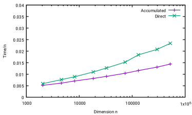
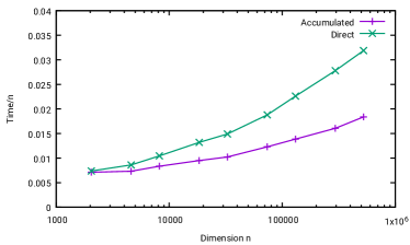
Figure 9: Runtime per degree of freedom for the $\mathcal{H}$-matrix multiplication, single layer $VV$ on the left, double layer $KK$ on the right

In a first experiment, we measure the runtime of the matrix multiplication algorithms with a truncation tolerance of $10^{-4}$. Figure 9 shows the runtime divided by the matrix dimension $n$ using a logarithmic scale for the $n$ axis. Both algorithms reach a relative accuracy well below $10^{-4}$ with respect to the spectral norm, and we can see that the version with accumulated updates has a significant advantage over the standard direct approach, particularly for large matrices. Although accumulating the updates requires additional truncation steps, the measured total error is not significantly larger. Since the new algorithm stores only one low-rank matrix for each ancestor of the current block, the temporary storage requirements are negligible.

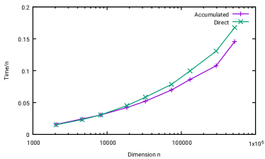
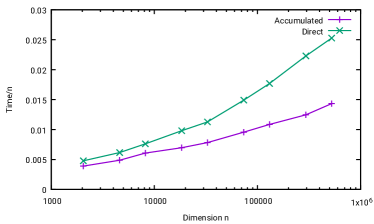
Figure 10: Runtime per degree of freedom for the $\mathcal{H}$-matrix inversion, single layer $V^{-1}$ on the left, double layer $K^{-1}$ on the right

In the next experiment, we consider the $\mathcal{H}$-matrix inversion, again using a truncation tolerance of $10^{-4}$. Since the inverse is frequently used as a preconditioner, we estimate the spectral norm $\|I-\widetilde{G}^{-1}G\|_{2}$ using a power iteration. For the single layer matrix $V$, this “preconditioner error” starts at $6\times 10^{-4}$ for the smallest matrix and grows to $10^{-2}$ for the largest, as is to be expected due to the increasing condition number. For the double layer matrix $K$, the error lies between $2\times 10^{-2}$ and $1.1\times 10^{-1}$. For $n=73\,728$, the error obtained by using accumulated updates is almost four times larger than the one for the classical algorithm, while for $n=524\,288$ both differ by only $13$ percent. We can see in Figure 10 that accumulated updates again reduce the runtime, but the effect is only very minor for the single layer matrix and far more pronounced for the double layer matrix.

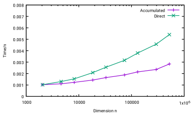
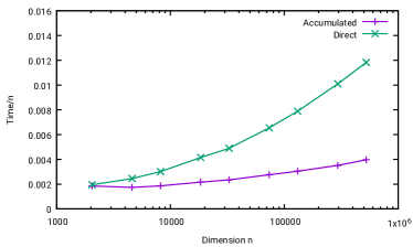
Figure 11: Runtime per degree of freedom for the $\mathcal{H}$-matrix factorization, single layer $LL^{*}=V$ on the left, double layer $LR=K$ on the right

In a final experiment, we investigate $\mathcal{H}$-matrix factorizations. Since $V$ is symmetric and positive definite, we approximate its Cholesky factorization $V\approx\widetilde{L}\widetilde{L}^{*}$, while we use the standard LR factorization $K\approx\widetilde{L}\widetilde{R}$ for the matrix $K$. The estimated preconditioner error $\|I-(\widetilde{L}\widetilde{L}^{*})^{-1}V\|_{2}$ for the single layer matrix of dimension $n=524\,288$ is close to $2.2\times 10^{-3}$ for the algorithm with accumulated updates and close to $9.5\times 10^{-4}$ for the standard algorithm. For the double layer matrix of the same dimension, the estimated error $\|I-(\widetilde{L}\widetilde{R})^{-1}K\|_{2}$ is close to $5.6\times 10^{-1}$ for the new algorithm and close to $3.8\times 10^{-1}$ for the standard algorithm. Figure 11 shows that accumulated updates significantly reduce the runtime for both factorizations.

In summary, accumulated updates reduce the runtime of the $\mathcal{H}$-matrix multiplication and factorization by a factor between two and three in our experiments while the error is only moderately increased. The same speed-up can be observed for the inversion of the double layer matrix, while the improvement for the single layer matrix is significantly smaller.

References

- [1] U. Baur. Low rank solution of data-sparse Sylvester equations. Numer. Lin. Alg. Appl., 15:837–851, 2008.
- [2] M. Bebendorf. Approximation of boundary element matrices. Numer. Math., 86(4):565–589, 2000.
- [3] M. Bebendorf and W. Hackbusch. Existence of -matrix approximants to the inverse FE-matrix of elliptic operators with -coefficients. Numer. Math., 95:1–28, 2003.
- [4] S. Börm. -matrix arithmetics in linear complexity. Computing, 77(1):1–28, 2006.
- [5] S. Börm. Approximation of solution operators of elliptic partial differential equations by - and -matrices. Numer. Math., 115(2):165–193, 2010.
- [6] S. Börm. Efficient Numerical Methods for Non-local Operators: -Matrix Compression, Algorithms and Analysis, volume 14 of EMS Tracts in Mathematics. EMS, 2010.
- [7] S. Börm and S. Christophersen. Approximation of integral operators by Green quadrature and nested cross approximation. Numer. Math., 133(3):409–442, 2016.
- [8] S. Börm and L. Grasedyck. Low-rank approximation of integral operators by interpolation. Computing, 72:325–332, 2004.
- [9] S. Börm and L. Grasedyck. Hybrid cross approximation of integral operators. Numer. Math., 101:221–249, 2005.
- [10] P. P. Ewald. Die Berechnung optischer und elektrostatischer Gitterpotentiale. Annalen der Physik, 369(3):253–287, 1920.
- [11] M. Faustmann, J. M. Melenk, and D. Praetorius. -matrix approximability of the inverse of FEM matrices. Numer. Math., 131(4):615–642, 2015.
- [12] I. Gavrilyuk, W. Hackbusch, and B. N. Khoromskij. -matrix approximation for the operator exponential with applications. Numer. Math., 92:83–111, 2002.
- [13] I. Gavrilyuk, W. Hackbusch, and B. N. Khoromskij. Data-sparse approximation to operator-valued functions of elliptic operator. Mathematics of Computation, 73:1107–1138, 2004.
- [14] L. Grasedyck. Existence of a low-rank or -matrix approximant to the solution of a Sylvester equation. Numer. Lin. Alg. Appl., 11:371–389, 2004.
- [15] L. Grasedyck and W. Hackbusch. Construction and arithmetics of -matrices. Computing, 70:295–334, 2003.
- [16] L. Grasedyck, W. Hackbusch, and B. N. Khoromskij. Solution of large scale algebraic matrix Riccati equations by use of hierarchical matrices. Computing, 70:121–165, 2003.
- [17] L. Grasedyck, R. Kriemann, and S. LeBorne. Parallel black box -LU preconditioning for elliptic boundary value problems. Comp. Vis. Sci., 11:273–291, 2008.
- [18] L. Grasedyck, R. Kriemann, and S. LeBorne. Domain decomposition based -LU preconditioning. Numer. Math., 112(4):565–600, 2009.
- [19] L. Grasedyck and S. LeBorne. -matrix preconditioners in convection-dominated problems. SIAM J. Mat. Anal., 27(4):1172–1183, 2006.
- [20] L. Greengard and V. Rokhlin. A fast algorithm for particle simulations. J. Comp. Phys., 73:325–348, 1987.
- [21] L. Greengard and V. Rokhlin. On the numerical solution of two-point boundary value problems. Comm. Pure Appl. Math., 44(4):419–452, 1991.
- [22] W. Hackbusch. A sparse matrix arithmetic based on -matrices. Part I: Introduction to -matrices. Computing, 62(2):89–108, 1999.
- [23] W. Hackbusch. Hierarchical Matrices: Algorithms and Analysis. Springer, 2015.
- [24] W. Hackbusch and Z. P. Nowak. On the fast matrix multiplication in the boundary element method by panel clustering. Numer. Math., 54(4):463–491, 1989.
- [25] M. Lintner. The eigenvalue problem for the 2d Laplacian in -matrix arithmetic and application to the heat and wave equation. Computing, 72:293–323, 2004.
- [26] V. Rokhlin. Rapid solution of integral equations of classical potential theory. J. Comp. Phys., 60:187–207, 1985.
- [27] S. A. Sauter. Variable order panel clustering. Computing, 64:223–261, 2000.