M. Ablikim1, M. N. Achasov9,d, S. Ahmed14, X. C. Ai1, O. Albayrak5, M. Albrecht4, D. J. Ambrose45, A. Amoroso50A,50C, F. F. An1, Q. An47,38, J. Z. Bai1, O. Bakina23, R. Baldini Ferroli20A, Y. Ban31, D. W. Bennett19, J. V. Bennett5, N. Berger22, M. Bertani20A, D. Bettoni21A, J. M. Bian44, F. Bianchi50A,50C, E. Boger23,b, I. Boyko23, R. A. Briere5, H. Cai52, X. Cai1,38, O. Cakir41A, A. Calcaterra20A, G. F. Cao1,42, S. A. Cetin41B, J. Chai50C, J. F. Chang1,38, G. Chelkov23,b,c, G. Chen1, H. S. Chen1,42, J. C. Chen1, M. L. Chen1,38, S. Chen42, S. J. Chen29, X. Chen1,38, X. R. Chen26, Y. B. Chen1,38, X. K. Chu31, G. Cibinetto21A, H. L. Dai1,38, J. P. Dai34,h, A. Dbeyssi14, D. Dedovich23, Z. Y. Deng1, A. Denig22, I. Denysenko23, M. Destefanis50A,50C, F. De Mori50A,50C, Y. Ding27, C. Dong30, J. Dong1,38, L. Y. Dong1,42, M. Y. Dong1,38,42, Z. L. Dou29, S. X. Du54, P. F. Duan1, J. Z. Fan40, J. Fang1,38, S. S. Fang1,42, X. Fang47,38, Y. Fang1, R. Farinelli21A,21B, L. Fava50B,50C, F. Feldbauer22, G. Felici20A, C. Q. Feng47,38, E. Fioravanti21A, M. Fritsch22,14, C. D. Fu1, Q. Gao1, X. L. Gao47,38, Y. Gao40, Z. Gao47,38, I. Garzia21A, K. Goetzen10, L. Gong30, W. X. Gong1,38, W. Gradl22, M. Greco50A,50C, M. H. Gu1,38, Y. T. Gu12, Y. H. Guan1, A. Q. Guo1, L. B. Guo28, R. P. Guo1, Y. Guo1, Y. P. Guo22, Z. Haddadi25, A. Hafner22, S. Han52, X. Q. Hao15, F. A. Harris43, K. L. He1,42, F. H. Heinsius4, T. Held4, Y. K. Heng1,38,42, T. Holtmann4, Z. L. Hou1, C. Hu28, H. M. Hu1,42, T. Hu1,38,42, Y. Hu1, G. S. Huang47,38, J. S. Huang15, X. T. Huang33, X. Z. Huang29, Z. L. Huang27, T. Hussain49, W. Ikegami Andersson51, Q. Ji1, Q. P. Ji15, X. B. Ji1,42, X. L. Ji1,38, L. L. Jiang1,L. W. Jiang52, X. S. Jiang1,38,42, X. Y. Jiang30, J. B. Jiao33, Z. Jiao17, D. P. Jin1,38,42, S. Jin1,42, T. Johansson51, A. Julin44, N. Kalantar-Nayestanaki25, X. L. Kang1, X. S. Kang30, M. Kavatsyuk25, B. C. Ke5, P. Kiese22, R. Kliemt10, B. Kloss22, O. B. Kolcu41B,f, B. Kopf4, M. Kornicer43, A. Kupsc51, W. Kühn24, J. S. Lange24, M. Lara19, P. Larin14, H. Leithoff22, C. Leng50C, C. Li51, Cheng Li47,38, D. M. Li54, F. Li1,38, F. Y. Li31, G. Li1, H. B. Li1,42, H. J. Li1, J. C. Li1, Jin Li32, K. Li13, K. Li33, Lei Li3, P. R. Li42,7, Q. Y. Li33, T. Li33, W. D. Li1,42, W. G. Li1, X. L. Li33, X. N. Li1,38, X. Q. Li30, Y. B. Li2, Z. B. Li39, H. Liang47,38, Y. F. Liang36, Y. T. Liang24, G. R. Liao11, D. X. Lin14, B. Liu34,h, B. J. Liu1, C. L. Liu5, C. X. Liu1, D. Liu47,38, F. H. Liu35, Fang Liu1, Feng Liu6, H. B. Liu12, H. H. Liu1, H. H. Liu16, H. M. Liu1,42, J. Liu1, J. B. Liu47,38, J. P. Liu52, J. Y. Liu1, K. Liu40, K. Y. Liu27, L. D. Liu31, P. L. Liu1,38, Q. Liu42, S. B. Liu47,38, X. Liu26, Y. B. Liu30, Y. Y. Liu30, Z. A. Liu1,38,42, Zhiqing Liu22, H. Loehner25, Y. F. Long31, X. C. Lou1,38,42, H. J. Lu17, J. G. Lu1,38, Y. Lu1, Y. P. Lu1,38, C. L. Luo28, M. X. Luo53, T. Luo43, X. L. Luo1,38, X. R. Lyu42, F. C. Ma27, H. L. Ma1, L. L. Ma33, M. M. Ma1, Q. M. Ma1, T. Ma1, X. N. Ma30, X. Y. Ma1,38, Y. M. Ma33, F. E. Maas14, M. Maggiora50A,50C, Q. A. Malik49, Y. J. Mao31, Z. P. Mao1, S. Marcello50A,50C, J. G. Messchendorp25, G. Mezzadri21B, J. Min1,38, T. J. Min1, R. E. Mitchell19, X. H. Mo1,38,42, Y. J. Mo6, C. Morales Morales14, G. Morello20A, N. Yu. Muchnoi9,d, H. Muramatsu44, P. Musiol4, Y. Nefedov23, F. Nerling10, I. B. Nikolaev9,d, Z. Ning1,38, S. Nisar8, S. L. Niu1,38, X. Y. Niu1, S. L. Olsen32, Q. Ouyang1,38,42, S. Pacetti20B, Y. Pan47,38, M. Papenbrock51, P. Patteri20A, M. Pelizaeus4, H. P. Peng47,38, K. Peters10,g, J. Pettersson51, J. L. Ping28, R. G. Ping1,42, R. Poling44, V. Prasad1, H. R. Qi2, M. Qi29, S. Qian1,38, C. F. Qiao42, L. Q. Qin33, N. Qin52, X. S. Qin1, Z. H. Qin1,38, J. F. Qiu1, K. H. Rashid49,i, C. F. Redmer22, M. Ripka22, G. Rong1,42, Ch. Rosner14, X. D. Ruan12, A. Sarantsev23,e, M. Savrié21B, C. Schnier4, K. Schoenning51, W. Shan31, M. Shao47,38, C. P. Shen2, P. X. Shen30, X. Y. Shen1,42, H. Y. Sheng1, W. M. Song1, X. Y. Song1, S. Sosio50A,50C, S. Spataro50A,50C, G. X. Sun1, J. F. Sun15, S. S. Sun1,42, X. H. Sun1, Y. J. Sun47,38, Y. Z. Sun1, Z. J. Sun1,38, Z. T. Sun19, C. J. Tang36, X. Tang1, I. Tapan41C, E. H. Thorndike45, M. Tiemens25, I. Uman41D, G. S. Varner43, B. Wang30, B. L. Wang42, D. Wang31, D. Y. Wang31, K. Wang1,38, L. L. Wang1, L. S. Wang1, M. Wang33, P. Wang1, P. L. Wang1, W. Wang1,38, W. P. Wang47,38, X. F. Wang40, Y. Wang37, Y. D. Wang14, Y. F. Wang1,38,42, Y. Q. Wang22, Z. Wang1,38, Z. G. Wang1,38, Z. H. Wang47,38, Z. Y. Wang1, Z. Y. Wang1, T. Weber22, D. H. Wei11, P. Weidenkaff22, S. P. Wen1, U. Wiedner4, M. Wolke51, L. H. Wu1, L. J. Wu1, Z. Wu1,38, L. Xia47,38, L. G. Xia40, Y. Xia18, D. Xiao1, H. Xiao48, Z. J. Xiao28, Y. G. Xie1,38, Y. H. Xie6, Q. L. Xiu1,38, G. F. Xu1, J. J. Xu1, L. Xu1, Q. J. Xu13, Q. N. Xu42, X. P. Xu37, L. Yan50A,50C, W. B. Yan47,38, W. C. Yan47,38, Y. H. Yan18, H. J. Yang34,h, H. X. Yang1, L. Yang52, Y. X. Yang11, M. Ye1,38, M. H. Ye7, J. H. Yin1, Z. Y. You39, B. X. Yu1,38,42, C. X. Yu30, J. S. Yu26, C. Z. Yuan1,42, Y. Yuan1, A. Yuncu41B,a, A. A. Zafar49, Y. Zeng18, Z. Zeng47,38, B. X. Zhang1, B. Y. Zhang1,38, C. C. Zhang1, D. H. Zhang1, H. H. Zhang39, H. Y. Zhang1,38, J. Zhang1, J. J. Zhang1, J. L. Zhang1, J. Q. Zhang1, J. W. Zhang1,38,42, J. Y. Zhang1, J. Z. Zhang1,42, K. Zhang1, L. Zhang1, S. Q. Zhang30, X. Y. Zhang33, Y. Zhang1, Y. Zhang1, Y. H. Zhang1,38, Y. N. Zhang42, Y. T. Zhang47,38, Yu Zhang42, Z. H. Zhang6, Z. P. Zhang47, Z. Y. Zhang52, G. Zhao1, J. W. Zhao1,38, J. Y. Zhao1, J. Z. Zhao1,38, Lei Zhao47,38, Ling Zhao1, M. G. Zhao30, Q. Zhao1, Q. W. Zhao1, S. J. Zhao54, T. C. Zhao1, Y. B. Zhao1,38, Z. G. Zhao47,38, A. Zhemchugov23,b, B. Zheng48,14, J. P. Zheng1,38, W. J. Zheng33, Y. H. Zheng42, B. Zhong28, L. Zhou1,38, X. Zhou52, X. K. Zhou47,38, X. R. Zhou47,38, X. Y. Zhou1, K. Zhu1, K. J. Zhu1,38,42, S. Zhu1, S. H. Zhu46, X. L. Zhu40, Y. C. Zhu47,38, Y. S. Zhu1,42, Z. A. Zhu1,42, J. Zhuang1,38, L. Zotti50A,50C, B. S. Zou1, J. H. Zou1(BESIII Collaboration)1 Institute of High Energy Physics, Beijing 100049, People’s Republic of China
2 Beihang University, Beijing 100191, People’s Republic of China
3 Beijing Institute of Petrochemical Technology, Beijing 102617, People’s Republic of China
4 Bochum Ruhr-University, D-44780 Bochum, Germany
5 Carnegie Mellon University, Pittsburgh, Pennsylvania 15213, USA
6 Central China Normal University, Wuhan 430079, People’s Republic of China
7 China Center of Advanced Science and Technology, Beijing 100190, People’s Republic of China
8 COMSATS Institute of Information Technology, Lahore, Defence Road, Off Raiwind Road, 54000 Lahore, Pakistan
9 G.I. Budker Institute of Nuclear Physics SB RAS (BINP), Novosibirsk 630090, Russia
10 GSI Helmholtzcentre for Heavy Ion Research GmbH, D-64291 Darmstadt, Germany
11 Guangxi Normal University, Guilin 541004, People’s Republic of China
12 Guangxi University, Nanning 530004, People’s Republic of China
13 Hangzhou Normal University, Hangzhou 310036, People’s Republic of China
14 Helmholtz Institute Mainz, Johann-Joachim-Becher-Weg 45, D-55099 Mainz, Germany
15 Henan Normal University, Xinxiang 453007, People’s Republic of China
16 Henan University of Science and Technology, Luoyang 471003, People’s Republic of China
17 Huangshan College, Huangshan 245000, People’s Republic of China
18 Hunan University, Changsha 410082, People’s Republic of China
19 Indiana University, Bloomington, Indiana 47405, USA
20 (A)INFN Laboratori Nazionali di Frascati, I-00044, Frascati, Italy; (B)INFN and University of Perugia, I-06100, Perugia, Italy
21 (A)INFN Sezione di Ferrara, I-44122, Ferrara, Italy; (B)University of Ferrara, I-44122, Ferrara, Italy
22 Johannes Gutenberg University of Mainz, Johann-Joachim-Becher-Weg 45, D-55099 Mainz, Germany
23 Joint Institute for Nuclear Research, 141980 Dubna, Moscow region, Russia
24 Justus-Liebig-Universitaet Giessen, II. Physikalisches Institut, Heinrich-Buff-Ring 16, D-35392 Giessen, Germany
25 KVI-CART, University of Groningen, NL-9747 AA Groningen, The Netherlands
26 Lanzhou University, Lanzhou 730000, People’s Republic of China
27 Liaoning University, Shenyang 110036, People’s Republic of China
28 Nanjing Normal University, Nanjing 210023, People’s Republic of China
29 Nanjing University, Nanjing 210093, People’s Republic of China
30 Nankai University, Tianjin 300071, People’s Republic of China
31 Peking University, Beijing 100871, People’s Republic of China
32 Seoul National University, Seoul, 151-747 Korea
33 Shandong University, Jinan 250100, People’s Republic of China
34 Shanghai Jiao Tong University, Shanghai 200240, People’s Republic of China
35 Shanxi University, Taiyuan 030006, People’s Republic of China
36 Sichuan University, Chengdu 610064, People’s Republic of China
37 Soochow University, Suzhou 215006, People’s Republic of China
38 State Key Laboratory of Particle Detection and Electronics, Beijing 100049, Hefei 230026, People’s Republic of China
39 Sun Yat-Sen University, Guangzhou 510275, People’s Republic of China
40 Tsinghua University, Beijing 100084, People’s Republic of China
41 (A)Ankara University, 06100 Tandogan, Ankara, Turkey; (B)Istanbul Bilgi University, 34060 Eyup, Istanbul, Turkey; (C)Uludag University, 16059 Bursa, Turkey; (D)Near East University, Nicosia, North Cyprus, Mersin 10, Turkey
42 University of Chinese Academy of Sciences, Beijing 100049, People’s Republic of China
43 University of Hawaii, Honolulu, Hawaii 96822, USA
44 University of Minnesota, Minneapolis, Minnesota 55455, USA
45 University of Rochester, Rochester, New York 14627, USA
46 University of Science and Technology Liaoning, Anshan 114051, People’s Republic of China
47 University of Science and Technology of China, Hefei 230026, People’s Republic of China
48 University of South China, Hengyang 421001, People’s Republic of China
49 University of the Punjab, Lahore-54590, Pakistan
50 (A)University of Turin, I-10125, Turin, Italy; (B)University of Eastern Piedmont, I-15121, Alessandria, Italy; (C)INFN, I-10125, Turin, Italy
51 Uppsala University, Box 516, SE-75120 Uppsala, Sweden
52 Wuhan University, Wuhan 430072, People’s Republic of China
53 Zhejiang University, Hangzhou 310027, People’s Republic of China
54 Zhengzhou University, Zhengzhou 450001, People’s Republic of China
a Also at Bogazici University, 34342 Istanbul, Turkey
b Also at the Moscow Institute of Physics and Technology, Moscow 141700, Russia
c Also at the Functional Electronics Laboratory, Tomsk State University, Tomsk, 634050, Russia
d Also at the Novosibirsk State University, Novosibirsk, 630090, Russia
e Also at the NRC ”Kurchatov Institute”, PNPI, 188300, Gatchina, Russia
f Also at Istanbul Arel University, 34295 Istanbul, Turkey
g Also at Goethe University Frankfurt, 60323 Frankfurt am Main, Germany
h Also at Key Laboratory for Particle Physics, Astrophysics and Cosmology, Ministry of Education; Shanghai Key Laboratory for Particle Physics and Cosmology; Institute of Nuclear and Particle Physics, Shanghai 200240, People’s Republic of China
i Government College Women University, Sialkot - 51310. Punjab, Pakistan.
Abstract
Using 2.93 fb-1 of data taken at 3.773 GeV with the BESIII detector operated
at the BEPCII collider, we study the semileptonic decays and
. We measure the absolute decay branching fractions
and
,
where the first uncertainties are statistical and the second systematic.
We also measure the differential decay rates
and study the form factors of these two decays.
With the values of and from Particle Data Group fits assuming CKM unitarity,
we obtain the values of the form factors at ,
and
.
Taking input from recent lattice QCD calculations of these form factors,
we determine values of the CKM matrix elements
and
,
where the third uncertainties are theoretical.
pacs:
13.20.Fc, 12.15.Hh
I Introduction
In the Standard Model (SM) of particle physics, the mixing between the
quark flavours in the weak interaction is parameterized by the Cabibbo-Kobayashi-Maskawa (CKM) matrix, which
is a unitary matrix.
Since the CKM matrix elements are fundamental parameters of the SM,
precise determinations of these elements are very important for tests
of the SM and searches for New Physics (NP) beyond the SM.
Since the effects of strong and weak interactions can be well separated in
semileptonic decays, these decays are excellent processes from which we can determine the magnitude of the CKM matrix element .
In the SM, neglecting the lepton mass, the differential decay rate for
( or ) is given by Z_Phys_C_46_93
(1)
where
is the Fermi constant,
is the corresponding CKM matrix element,
is the momentum of the meson in the rest frame of the meson,
is the squared four momentum transfer,
i.e., the invariant mass of the lepton and neutrino system,
and is the form factor which parameterizes the effect of the strong interaction.
In Eq. (1), is a multiplicative factor due to isospin,
which equals to 1 for the decay and for the decay .
In this article, we report the experimental study of
and decays
using a 2.93 fb-1lum data set collected at a center-of-mass energy of
GeV with the BESIII detector operated at the BEPCII collider.
Throughout this paper, the inclusion of charge conjugate
channels is implied.
The paper is structured as follows.
We briefly describe the BESIII detector and the Monte Carlo (MC) simulation in Sec. II.
The event selection is presented in Sec. III.
The measurements of the absolute branching fractions and the differential decay rates
are described in Sec. IV and V, respectively.
In Sec. VI we discuss the determination of form factors from the
measurements of decay rates, and finally, in Sec. VII, we present
the determination of the magnitudes of the CKM matrix elements and .
A brief summary is given in Sec. VIII.
II BESIII detector
The BESIII detector is a cylindrical detector with a
solid-angle coverage of of ,
designed for the study of hadron spectroscopy and -charm physics.
The BESIII detector is described in detail in Ref. bes3 .
Detector components particularly relevant for this work are
(1) the main drift chamber (MDC) with 43 layers surrounding the beam pipe,
which performs precise determination of charged particle
trajectories and provides a measurement of the specific ionization energy loss ();
(2) a time-of-flight system (TOF) made of plastic scintillator counters, which are located outside of
the MDC and provide additional charged particle identification
information;
and (3) the electromagnetic calorimeter (EMC) consisting of 6240 CsI(Tl) crystals,
used to measure the energy of photons and to identify electrons.
A geant4-based geant4 MC simulation software BOOST ,
which contains the detector geometry description and the detector response,
is used to optimize the event selection criteria, study possible backgrounds,
and determine the reconstruction efficiencies.
The production of the ,
initial state radiation production of and ,
as well as the continuum processes of
and () are simulated
by the MC event generator kkmckkmc ;
the known decay modes are generated by evtgenbesevtgen
with the branching fractions set to the world average values from the
Particle Data Group (PDG) pdg2016 ;
while the remaining unknown decay modes are modeled by
lundcharmlundcharm .
We also generate signal MC events consisting of
events in which the meson
decays to all possible final states
and the meson decays to a hadronic
or a semileptonic decay final state being investigated.
In the generation of signal MC events,
the semileptonic decays and
are modeled by the the modified pole parametrization (see Sec. VI.1).
III Event reconstruction
The center-of-mass energy of 3.773 GeV corresponds to
the peak of the resonance, which decays predominantly
into ( or ) meson pairs.
In events where a meson is fully reconstructed,
the remaining particles must all be decay
products of the accompanying meson. In the following, the
reconstructed meson is called “tagged ” or “ tag”.
In a tagged data sample, the recoiling decays to
or can be cleanly isolated and used to measure the branching fraction and
differential decay rates.
III.1 Selection of tags
We reconstruct tags in the following nine hadronic modes:
, , , ,
, 111
We veto the candidates when a invariant mass
falls within the mass window.
, ,
, and .
The selection criteria of tags used here are the same as those described in
Ref. BESIII_Dptomunu .
Tagged mesons are identified by their beam-energy-constrained mass
,
where is the beam energy,
and is the measured 3-momentum of the tag candidate 222
In this analysis, all four-momentum vectors measured
in the laboratory frame are boosted to the center-of-mass
frame.
.
We also use the variable ,
where is the measured energy of the tag candidate,
to select the tags.
Each tag candidate is subjected to a tag mode-dependent requirement as shown in Table 1.
If there are multiple candidates per tag mode for an event,
the one with the smallest value of is retained.
Table 1:
The requirements, the signal regions,
the yields of the tags () reconstructed in data,
and the reconstruction efficiency () of tags.
The uncertainties are statistical only.
Tag mode
(MeV)
(GeV)
(%)
Sum
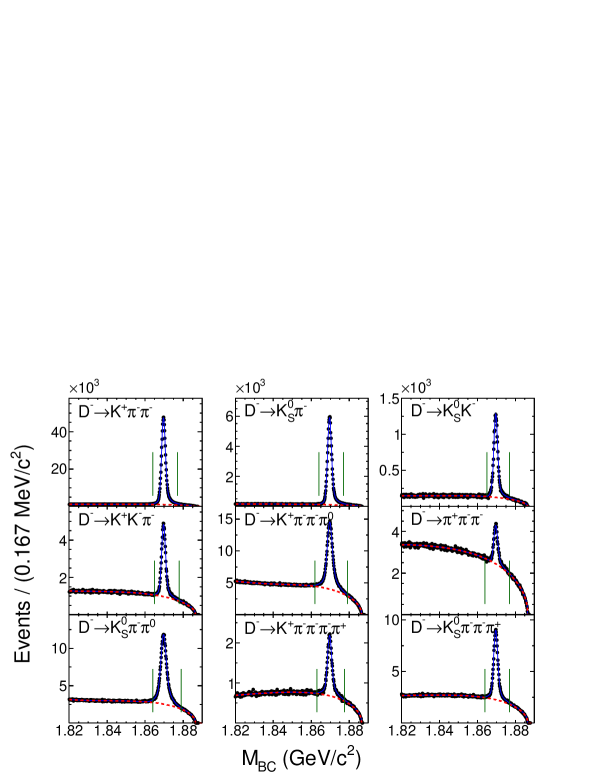
The distributions for the nine tag modes are shown in Fig. 1.
A binned extended maximum likelihood fit is used to determine the number of tagged events
for each of the nine modes.
We use the MC simulated signal shape
convolved with a double-Gaussian resolution function to represent
the beam-energy-constrained mass signal for the daughter particles, and
an ARGUS function Albrecht-1990am multiplied by a third-order polynomial BESII_D0toPenu ; BESIII_D0toPenu
to describe the background shape for the distributions.
In the fits all parameters of the double-Gaussian function,
the ARGUS function, and the polynomial function are left free.
The solid lines in Fig. 1 show the best fits, while the dashed
lines show the fitted background shapes.
The numbers of the tags ()
within the signal regions
given by the two vertical lines in Fig. 1
are summarized in Table 1.
In total, we find single tags reconstructed in data.
The reconstruction efficiencies of the single tags, ,
as determined with the MC simulation, are shown in Table 1.
Figure 1:
Fits (solid lines) to the distributions (points with error bars)
in data for nine tag modes.
The two vertical lines show the tagged mass regions.
III.2 Reconstruction of semileptonic decays
Candidates for semileptonic decays are selected from the remaining tracks in the system recoiling against the tags.
The , TOF and EMC measurements (deposited energy and shape of the electromagnetic shower) are combined to form confidence levels for
the hypothesis (), the hypothesis (), and the hypothesis ().
Positron candidates are required to have greater than 0.1% and to satisfy .
In addition, we include the 4-momenta of near-by photons
within of
the direction of the positron momentum
to partially account for final-state-radiation energy losses (FSR recovery).
The neutral kaon candidates are built from pairs of oppositely charged tracks that
are assumed to be pions.
For each pair of charged tracks, a vertex fit is performed and
the resulting track parameters are used to calculate the invariant mass, .
If is in the range (0.484, 0.512) GeV, the
pair is treated as a candidate and is used for further analysis.
The neutral pion candidates are reconstructed via the decays.
For the photon selection, we require
the energy of the shower deposited
in the barrel (end-cap) EMC greater than
25 (50) MeV and
the shower time be within 700 ns of the event start time.
In addition, the angle between the photon and the
nearest charged track is required to be greater than .
We accept the pair of photons as a candidate
if the invariant mass of the two photons, ,
is in the range (0.110, 0.150) GeV.
A 1-Constraint (1-C) kinematic fit is then performed to constrain
to the nominal mass,
and the resulting 4-momentum of the candidate is used for further analysis.
We reconstruct the decay by requiring exactly three
additional charged tracks in the rest of the event. One track with charge opposite to
that of the tag is identified as
a positron using the criteria mentioned above,
while the other two oppositely charged
tracks form a candidate.
For the selection of the decay, we require that
there is only one additional charged track consistent with the positron
identification criteria and at least two photons that are used to form a
candidate in the rest of the event. If there are
multiple candidates,
the one with the minimum from the 1-C kinematic fit is retained.
In order to additionally suppress background due to wrongly reconstructed or background photons,
the semileptonic candidate is further required to have
the maximum energy of any of the unused photons, , less than 300 MeV.
Since the neutrino is undetected,
the kinematic variable
is used to obtain the information about the missing neutrino,
where and are, respectively, the total missing energy
and momentum in the event.
The missing energy is computed from ,
where
and are the measured energies of the pseudoscalar meson and the positron, respectively.
The missing momentum is given by ,
where , and are
the 3-momenta of the meson, the pseudoscalar meson and the positron, respectively.
The 3-momentum of the meson is taken as
,
where is the direction of the momentum of the single tag,
and is the mass.
If the daughter particles from a semileptonic decay are correctly identified,
is near zero, since only one neutrino is missing.
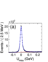
Figure 2 shows the distributions for the semileptonic candidates,
where the potential backgrounds arise from the processes other than signal,
non- decays, ,
continuum light hadron production, initial state radiation return to and .
The background for is dominated by
and .
For , the background is mainly from
and .
Figure 2:
Distributions of for the selected (a) and (b) candidates (points with error bars) with fit projections overlaid (solid lines). The dashed curves show the background determined by the fit.
Following the same procedure described in Ref. BESIII_D0toPenu ,
we perform a binned extended maximum likelihood fit to the distribution for each
channel to separate the signal from the background component.
The signal shape is constructed from a convolution of a MC determined distribution and a Gaussian function that accounts for the difference of the
resolutions between data and MC simulation.
The background shape is formed from MC simulation.
From the fits shown as the overlaid curves in Fig. 2,
we obtain the yields of the observed signal events to be
and
, respectively.
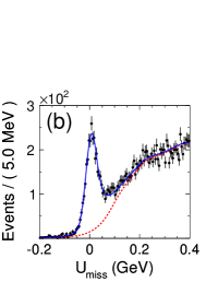
To check the quality of the MC simulation,
we examine the distributions of the reconstructed kinematic variables.
Figure 3 shows the comparisons of the momentum distributions of
data and MC simulation.
Figure 3:
Momentum distributions of selected events (with MeV)
for (a) , (b) from ,
(c) , and (d) from .
The points with error bars represent data,
the (blue) open histograms are MC simulated signal plus background,
the shaded histograms are MC simulated background only.
IV Branching fraction measurements
IV.1 Determinations of branching fractions
The branching fraction of the semileptonic decay is
obtained from
(2)
where is the number of tags (see Sec. III.1),
is the number of observed decays
within the tags (see Sec. III.2), and
is the reconstruction efficiency.
Here the efficiency includes
the fraction of the and branching fraction,
the efficiency includes
the branching fraction pdg2016 .
Due to the difference in the multiplicity, the reconstruction efficiency varies slightly with the tag mode.
For each tag mode , the reconstruction efficiency is given by
,
where the efficiency for simultaneously finding
the semileptonic decay and the meson tagged with
mode , , is determined using the signal MC sample,
and is the corresponding tag efficiency shown in
Table 1.
These efficiencies are listed in Table 2.
The reconstruction efficiency for each tag mode is then weighted according to the
corresponding tag yield in data to obtain the average reconstruction efficiency,
,
as listed in the last row in Table 2.
Table 2:
The reconstruction efficiencies for and
determined from MC simulation.
The efficiencies include the branching fractions for and . The uncertainties are statistical only.
Tag mode
(%)
(%)
(%)
(%)
Average
Using the control samples selected from Bhabha scattering and events,
we find that there are small discrepancies between data and MC simulation in the
positron tracking efficiency, positron identification efficiency,
and reconstruction efficiencies.
We correct for these differences by multiplying the raw efficiencies
and
determined in MC simulation by factors of 0.9957 and 0.9910, respectively.
The corrected efficiencies are found to be
and
,
where the uncertainties are only statistical.
Inserting the corresponding numbers into Eq. (2)
yields the absolute decay branching fractions
(3)
and
(4)
where the first uncertainties are statistical and the second systematic.
IV.2 Systematic uncertainties
The systematic uncertainties in the measured branching fractions of
and decays
include the following contributions.
Number of tags.
The systematic uncertainty of the number of tags is 0.5% BESIII_Dptomunu .
tracking efficiency.
Using the positron samples selected from radiative Bhabha scattering events,
the tracking efficiencies are measured in data and MC simulation.
Considering both the polar angle and momentum distributions of the positrons
in the semileptonc decays,
a correction factor of ()
is determined for the tracking efficiency in the branching fraction measurement of () decay.
This correction is applied and an uncertainty of 0.19% (0.15%) is
used as the corresponding systematic uncertainty.
identification efficiency.
Using the positron samples selected from radiative Bhabha scattering events,
we measure the identification efficiencies in data and MC simulation.
Taking both the polar angle and momentum distributions of the positrons
in the semileptonic decays into account,
a correction factor of ()
is determined for the identification efficiency
in the measurement of
().
This correction is applied, and an amount of 0.16% (0.14%) is
assigned as the corresponding systematic uncertainty.
and reconstruction efficiency.
The momentum-dependent efficiencies for () reconstruction
in data and in MC simulation are measured with events.
Weighting these efficiencies according to the () momentum distribution
in the semileptonic decay
leads to a difference of () between
the () reconstruction efficiencies in data and MC simulation.
Since we correct for the systematic shift,
the uncertainty of the correction factor, (), is
taken as the corresponding systematic uncertainty in the measured
branching fraction of ().
Requirement on .
By comparing doubly tagged hadronic decay events in the data and MC
simulation, the systematic uncertainty due to this source is estimated to be 0.1%.
Fit to the distribution.
To estimate the uncertainties
due to the fits to the distributions,
we refit the distributions by varying the bin size and the tail parameters
(which are used to describe the signal shapes and are determined from MC simulation)
to obtain the number of signal events from semileptonic decays.
We then combine the changes in the yields in quadrature to obtain
the systematic uncertainty
(0.12% for , 0.52% for ).
Since the background function
is formed from many background modes with fixed relative
normalizations, we also vary the relative contributions of
several of the largest background modes based on the
uncertainties in their branching fractions
(0.12% for , 0.01% for ).
In addition, we convolute the background shapes formed from MC simulation
with the same Gaussian function in the fits
(0.02% for , 0.30% for ).
Finally we assign the relative uncertainties to be and for
and , respectively.
Form factor.
In order to estimate the systematic uncertainty associated with
the form factor used to generate signal events in the MC simulation,
we re-weight the signal MC events so that the spectra
agree with the measured spectra. We then remeasure the branching fraction
(partial decay rates in different bins)
with the newly weighted efficiency (efficiency matrix).
The maximum relative change of the branching fraction
(partial decay rates in different bins) is
and is assigned as the systematic uncertainty.
FSR recovery.
The differences between the results with FSR recovery and the ones without FSR
recovery are assigned as the systematic uncertainties due to FSR recovery.
We find the differences are and for
and , respectively.
MC statistics.
The uncertainties in the measured branching fractions due to the MC statistics are
the statistical fluctuation of the MC samples, which are for both of
and semileptonic decays.
and decay branching fractions.
We include an uncertainty of 0.07% (0.03%) on the branching fraction measurement
of ()
to account for the uncertainty of the branching fraction of
() decay pdg2016 .
Table 3:
Summary of the systematic uncertainties considered
in the measurements of the branching fractions of
and decays.
Systematic uncertainty (%)
Source
Number of tags
0.5
0.5
Tracking for
0.19
0.15
PID for
0.16
0.14
reconstruction
1.62
reconstruction
1.00
Requirement on
0.1
0.1
Fit to distribution
0.2
0.6
Form factor
0.2
0.2
FSR recovery
0.1
0.5
MC statistics
0.2
0.2
branching fraction
0.07
0.03
Total
1.76
1.41
Table 3 summarizes the systematic uncertainties
in the measurement of the branching fractions.
Adding all systematic uncertainties in quadrature yields the total systematic uncertainties
of and for and , respectively.
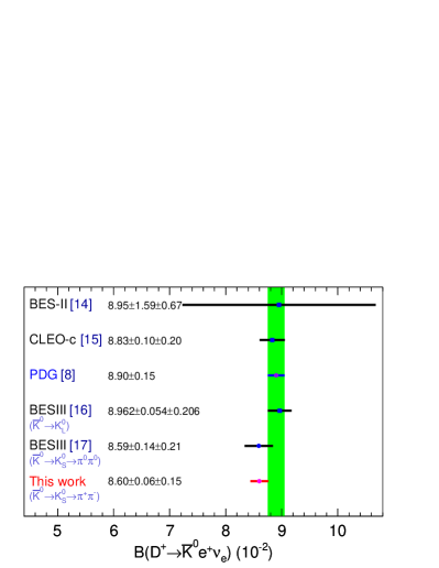
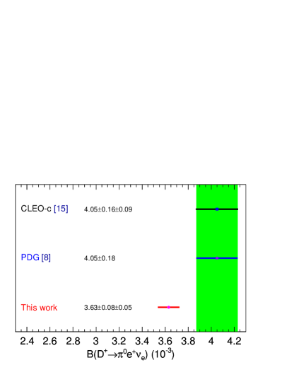
IV.3 Comparison
The comparisons of our measured branching fractions
for and
decays with those
previously measured at the
BES-II BESII_DptoK0enu ,
CLEO-c CLEOc_DtoPenu_818
and BESIII BESIII_DptoKLenu ; BESIII_DptoKSenu experiments
as well as the PDG values pdg2016
are shown in Fig. 4.
Our measured branching fractions are in agreement
with the other experimental measurements, but are more precise.
For , our result is lower than the only other existing measurement by CLEO-c CLEOc_DtoPenu_818 by .
Figure 4:
Comparison of the branching fraction measurements for
(left) and (right).
The green bands correspond to the limits of the world averages.
Using our previous measurements of and
BESIII_D0toPenu ,
the results obtained in this analysis,
and the lifetimes of and mesons pdg2016 ,
we obtain the ratios
(5)
and
(6)
which are consistent with isospin symmetry.
V Partial decay rate measurements
V.1 Determinations of partial decay rates
To study the differential decay rates,
we divide the semileptonic candidates satisfying the selection criteria described in
Sec. III into bins of . Nine (seven) bins are used for
(). The range of each bin is given in
Table 4.
The squared four momentum transfer is determined for each semileptonic candidate by
,
where the energy and momentum of the missing neutrino are taken to be
and
, respectively.
For each bin, we perform a maximum likelihood fit to the corresponding
distribution following the same procedure described in Sec. III.2 and obtain the signal yields as shown in Table 4.
Table 4:
Summary of the range of each bin,
the number of the observed signal events for and in data.
Bin No.
1
2
3
4
5
6
7
8
9
(GeV
Bin No.
1
2
3
4
5
6
7
(GeV
To account for detection efficiency and detector resolution,
the number of events observed in the th bin is
extracted from the relation
(7)
where
is the number of bins,
is the number of semileptonic decay events produced in the tagged
sample with the filled in the th bin, and
is the overall efficiency matrix that describes the efficiency
and smearing across bins.
The efficiency matrix element is obtained by
(8)
where is the number of the signal MC events generated in the th bin
and reconstructed in the th bin,
is the total number of the signal MC events which are generated in the th bin,
and is the matrix
to correct for data-MC differences in the efficiencies for tracking, identification,
and () reconstruction.
Table 5 presents the average overall efficiency matrices for and decays.
To produce this average overall efficiency matrix, we combine the efficiency matrices for
each tag mode weighted by its yield shown in Table 1.
The diagonal elements of the matrix give the overall efficiencies for decays
to be reconstructed in the correct bins in the recoil of the single tags,
while the neighboring off-diagonal elements of the matrix give the overall efficiencies
for cross feed between different bins.
Table 5:
Efficiency matrices given in percent for and decays. The column gives the true bin , while the row gives the reconstructed bin .
The statistical uncertainties in the least significant digits are given in the parentheses.
Rec.
True (GeV)
(GeV)
Rec.
True (GeV)
(GeV)
The partial decay width in the th bin is obtained by
inverting the matrix Eq. (7),
(9)
where is the lifetime of the meson pdg2016 .
The -dependent partial widths for and
are summarized in Table 6.
Also shown in Table 6 are the statistical uncertainties and
the associated correlation matrices.
Table 6: Summary of the measured partial decay rates, relative statistical uncertainties,
systematic uncertainties and corresponding correlation matrices
for and .
bin No.
1
2
3
4
5
6
7
8
9
(ns-1)
stat. uncert. (%)
stat. correl.
syst. uncert. (%)
syst. correl.
bin No.
1
2
3
4
5
6
7
(ns-1)
stat. uncert. (%)
stat. correl.
syst. uncert. (%)
syst. correl.
V.2 Systematic covariance matrices
For each source of systematic uncertainty in the measurements of partial decay rates,
we construct an systematic covariance matrix.
A brief description of each contribution follows.
lifetime.
The systematic uncertainty associated with the lifetime of the meson
(0.7%) pdg2016
is fully correlated across bins.
Number of tags.
The systematic uncertainty from the number of the single tags (0.5%)
is fully correlated between bins.
, , and reconstruction.
The covariance matrices for the systematic uncertainties associated with the
tracking, identification, , and reconstruction
efficiencies are obtained in the following way.
We first vary the corresponding correction factors according to
their uncertainties, then remeasure
the partial decay rates using the efficiency matrices determined from the re-corrected signal MC events.
The covariance matrix due to this source is assigned via
,
where denotes the change in the partial decay rate measurement in the th bin.
Requirement on .
We take the systematic uncertainty of due to the
requirement on the selected events in each bin,
and assume that this uncertainty is fully correlated between bins.
Fit to the distribution.
The technique of fitting the distributions affects the number of signal events observed in the bins.
The covariance matrix due to the fits is determined by
(10)
where is the systematic uncertainty of
associated with the fit to the corresponding distribution.
Form factor.
To estimate the systematic uncertainty associated with
the form factor model used to generate signal events in the MC simulation,
we re-weight the signal MC events so that the spectra
agree with the measured spectra.
We then re-calculate the partial decay rates in different bins
with the new efficiency matrices which are determined using the weighted
MC events. The covariance matrix due to this source is assigned via
,
where denotes the change of the partial width measurement in the th bin.
FSR recovery.
To estimate the systematic covariance matrix associated with the FSR recovery of the positron momentum,
we remeasure the partial decay rates without the FSR recovery.
The covariance matrix due to this source is assigned via
,
where denotes the change of the partial decay rate measurement in the th bin.
MC statistics.
The systematic uncertainties due to the limited size of the MC samples
used to determine the efficiency matrices are translated to the covariance via
(11)
where the covariance of the inverse efficiency matrix elements are given
by cov_inverse_matrix
(12)
and decay branching fractions.
The systematic uncertainties due to the branching fractions of
(0.07%) and
(0.03%) are fully correlated between bins.
The total systematic covariance matrix is obtained by summing all these matrices.
Table 6 summarizes
the relative size of systematic uncertainties and the corresponding
correlations in the measurements for the partial decay rates of the
and semileptonic decays.
VI Form Factors
To determine the product and
other form factor parameters,
we fit the measured partial decay rates using Eq. (1)
with the parameterization of the form factor .
In this analysis, we use several forms of the form factor
parameterizations which are reviewed in Sec. VI.1.
VI.1 Form factor parameterizations
In general, the single pole model is the simplest approach to describe the dependence of the form factor. The single pole model is expressed as
(13)
where is the value of the form factor at , and is the pole
mass, which is often treated as a free parameter to improve fit quality.
The modified pole modelBK is also widely used in Lattice QCD (LQCD) calculations
and experimental studies of these decays.
In this parameterization, the form factor
of the semileptonic decays is written as
(14)
where is the mass of the meson,
and is a free parameter to be fitted.
where is the kinematical limit of ,
and is the conventional radius of the meson.
The most general parameterization of the form factor is the series expansionff_zexpansion , which is based on analyticity and unitarity.
In this parameterization, the variable is mapped to a new variable through
(16)
with and .
The form factor is then expressed in terms of the new variable as
(17)
where are real coefficients.
The function is for and for .
The standard choice of is
(18)
where is the mass of the charm quark.
In practical use, one usually makes a truncation of the above series.
After optimizing the form factor parameters, we obtain
(19)
where .
In this analysis we fit the measured decay rates to the two- or three-parameter series expansion,
i.e., we take or .
In fact, the expansion with only a linear term is sufficient to describe the data.
Therefore we take the two-parameter series expansion as the
nominal parameterization to determine and .
VI.2 Fitting partial decay rates to extract form factors
In order to determine the form factor parameters,
we fit the theoretical parameterizations to the measured partial decay rates.
Taking into account the correlations of the measured partial decay rates among bins,
the to be minimized in the fit is defined as
(20)
where is the measured partial decay rate in the th bin,
is the inverse matrix of the covariance matrix
.
In the th bin, the theoretical expectation of the partial decay rate is
obtained by integrating Eq. (1),
(21)
where and are the lower
and upper boundaries of that bin, respectively.
In the fits, all parameters of the form factor parameterizations are left free.
The central values of the form factor parameters are taken from the results obtained by fitting the data
with the combined statistical and systematic covariance matrix together.
The quadratic difference between the uncertainties of the fit parameters
obtained from the fits with the combined covariance matrix
and
the uncertainties of the fit parameters
obtained from the fits with the statistical covariance matrix only
is taken as the systematic error of the measured form factor parameter.
The results of these fits are summarized
in Table 7,
where the first errors are statistical and the second systematic.
Table 7: Summary of results of form factor fits for and , where the first errors are statistical and the second systematic.
Single pole model
Decay mode
(GeV)
Modified pole model
Decay mode
ISGW2 model
Decay mode
(GeV)
Two-parameter series expansion
Decay mode
Three-parameter series expansion
Decay mode
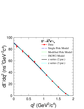
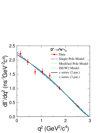
Figure 5:
Differential decay rates for (left)
and (right) as a function of .
The dots with error bars show the data
and the lines give the best fits to the data
with different form factor parameterizations.
Figure 5 shows the fits to the measured differential decay rates
for and .
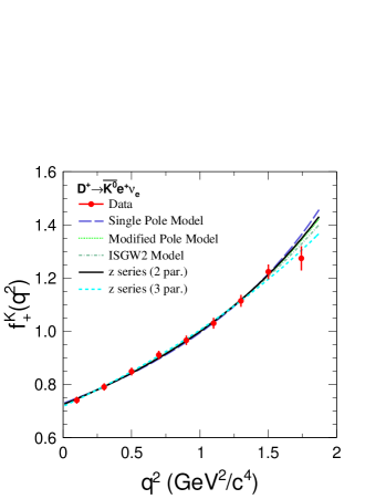
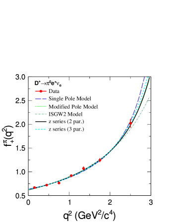
Figure 6 shows the projection of
the fits onto for the and
decays, respectively.
In these two figures, the dots with error bars show the measured values of
the form factors, , in the center of each bin, which are obtained with
(22)
in which
(23)
where
and
are taken from the SM constraint fit pdg2016 .
In the calculation of , is computed
using the two parameter series parameterization with the measured parameters.
Figure 6:
Projections on for (left)
and (right) as function of ,
where the dots with error bars show the data
and the lines give the best fits to the data
with different form factor parameterizations.
VI.3 Determinations of and
Using the values from the two-parameter
series expansion fits and
taking the values of from the SM constraint fit pdg2016 as inputs,
we obtain the form factors
(24)
and
(25)
where the first errors are statistical and the second systematic.
VII Determinations of and
Using the values of from the two-parameter
-series expansion fits
and in conjunction with the form factor values
LQCD_fK
and LQCD_fpi calculated from LQCD,
we obtain
(26)
and
(27)
where the first uncertainties are statistical,
the second systematic,
and the third are due to the theoretical uncertainties in
the LQCD calculations of the form factors.
VIII Summary
In summary, by analyzing 2.93 fb-1 of data collected at 3.773 GeV with the BESIII detector at the BEPCII,
the semileptonic decays for and have been studied.
From a total of tags, and
signal events are observed in the system recoiling against
the tags. These yield the absolute decay branching fractions to be
and
.
We also study the relations between the partial decay rates and squared 4-momentum transfer for these two decays
and obtain the parameters of different
form factor parameterizations.
The products of the form factors and the related CKM matrix elements
extracted from the two-parameter series expansion parameterization
are selected as our primary results. We obtain
and
.
Using the global SM fit values for and , we obtain the form factors
and
.
Furthermore, using the form factors predicted by the LQCD
calculations, we obtain the CKM matrix elements
and
,
where the third errors are dominated by the theoretical
uncertainties in the LQCD calculations of the form factors.
Acknowledgements.
The BESIII collaboration thanks the staff of BEPCII and the IHEP computing center for their strong support. This work is supported in part by National Key Basic Research Program of China under Contract Nos. 2009CB825204, 2015CB856700; National Natural Science Foundation of China (NSFC) under Contracts Nos. 10935007, 11235011, 11305180, 11322544, 11335008, 11425524, 11635010; the Chinese Academy of Sciences (CAS) Large-Scale Scientific Facility Program; the CAS Center for Excellence in Particle Physics (CCEPP); the Collaborative Innovation Center for Particles and Interactions (CICPI); Joint Large-Scale Scientific Facility Funds of the NSFC and CAS under Contracts Nos. U1232201, U1332201, U1532257, U1532258; CAS under Contracts Nos. KJCX2-YW-N29, KJCX2-YW-N45; 100 Talents Program of CAS; National 1000 Talents Program of China; INPAC and Shanghai Key Laboratory for Particle Physics and Cosmology; German Research Foundation DFG under Contracts Nos. Collaborative Research Center CRC 1044, FOR 2359; Istituto Nazionale di Fisica Nucleare, Italy; Koninklijke Nederlandse Akademie van Wetenschappen (KNAW) under Contract No. 530-4CDP03; Ministry of Development of Turkey under Contract No. DPT2006K-120470; The Swedish Resarch Council; U. S. Department of Energy under Contracts Nos. DE-FG02-05ER41374, DE-SC-0010118, DE-SC-0010504, DE-SC-0012069; U.S. National Science Foundation; University of Groningen (RuG) and the Helmholtzzentrum fuer Schwerionenforschung GmbH (GSI), Darmstadt; WCU Program of National Research Foundation of Korea under Contract No. R32-2008-000-10155-0.
References
(1)
J. G. Köerner and G. A. Schuler, Z. Phys. C 46, 93 (1990);
F. J. Gilman and R. L. Singleton, Jr., Phys. Rev. D 41, 142 (1990).
(2)
M. Ablikim et al. (BESIII Collaboration), Chin. Phys. C 37, 123001 (2013); Phys. Lett. B 753, 629 (2016).
(3)
M. Ablikim et al. (BESIII Collaboration), Nucl. Instrum. Methods Phys. Res., Sect. A 614, 345 (2010).
(4)
S. Agostinelli et al. (GEANT4 Collaboration), Nucl. Instrum.
Methods Phys. Res., Sect. A 506, 250 (2003).
(5)
Z. Y. Deng et al., Chin. Phys. C 30, 371 (2006).
(6)
S. Jadach, B. F. L. Ward, and Z. Was, Comput. Phys. Commun. 130, 260 (2000).
(7)
D. J. Lange, Nucl. Instrum. Meth. A 462, 152 (2001);
R.-G. Ping, Chin. Phys. C 32, 599 (2008).
(8)
C. Patrignani et al. (Particle Data Group), Chin. Phys. C 40, 100001 (2016).
(9)
J. C. Chen, G. S. Huang, X. R. Qi, D. H. Zhang and Y. S. Zhu, Phys. Rev. D 62, 034003 (2000).
(10)
M. Ablikim et al. (BESIII Collaboration), Phys. Rev. D 89, 051104(R) (2014).
(11)
H. Albrecht et al. (ARGUS Collaboration), Phys. Lett. B 241, 278 (1990).
(12)
M. Ablikim et al. (BES Collaboration), Phys. Lett. B 597, 39 (2004).
(13)
M. Ablikim et al. (BESIII Collaboration), Phys. Rev. D 92, 072012 (2015).
(14)
M. Ablikim et al. (BES Collaboration), Phys. Lett. B 608, 24 (2005).
(15)
D. Besson et al. (CLEO Collaboration), Phys. Rev. D 80, 032005 (2009).
(16)
M. Ablikim et al. (BESIII Collaboration), Phys. Rev. D 92, 112008 (2015).
(17)
M. Ablikim et al. (BESIII Collaboration), Chin. Phys. C 40, 113001 (2016).
(18)
M. Lefebvre, R.K. Keeler, R. Sobie, and J. White, Nucl. Instrum. Methods Phys. Res., Sect. A 451, 520 (2000).
(19)
D. Becirevcic and A. B. Kaidalov, Phys. Lett. B 478, 417 (2000).
(20)
D. Scora and N. Isgur, Phys. Rev. D 52, 2783 (1995).
(21)
T. Becher and R. J. Hill, Phys. Lett. B 633, 61 (2006).
(22)
H. Na et al. (HPQCD Collaboration), Phys. Rev. D 82, 114506 (2010).
(23)
H. Na et al. (HPQCD Collaboration), Phys. Rev. D 84, 114505 (2011).