Anomalous Hall effect and topological defects in antiferromagnetic Weyl semimetals: Mn₃Sn/Ge

Abstract

We theoretically study the interplay between bulk Weyl electrons and magnetic topological defects, including magnetic domains, domain walls, and $\mathbb{Z}_{6}$ vortex lines, in the antiferromagnetic Weyl semimetals Mn₃Sn and Mn₃Ge with negative vector chirality. We argue that these materials possess a hierarchy of energies scales which allows a description of the spin structure and spin dynamics using a XY model with $\mathbb{Z}_{6}$ anisotropy. We propose a dynamical equation of motion for the XY order parameter, which implies the presence of $\mathbb{Z}_{6}$ vortex lines, the double-domain pattern in the presence of magnetic fields, and the ability to control domains with current. We also introduce a minimal electronic model which allows efficient calculation of the electronic structure in the antiferromagnetic configuration, unveiling Fermi arcs at domain walls, and sharp quasi-bound states at $\mathbb{Z}_{6}$ vortices. Moreover, we have shown how these materials may allow electronic-based imaging of antiferromagnetic microstructure, and propose a possible device based on domain-dependent anomalous Hall effect.

The Hall effect has long been a nucleation center for geometry and topology in the physics of solids. In the 1950s, prescient work of Karplus and Luttinger identified Berry curvature of electron wavefunctions as the heart of the anomalous Hall effect (AHE) in ferromagnetsKarplus and Luttinger (1954); Nagaosa et al. (2010). In the 1980s, topology entered with the discovery of the quantum Hall effect. These ideas came together in the mid-2000s to unveil broad applications to electronic systems in the form of topological insulators, superconductors Hasan and Kane (2010); Qi and Zhang (2011) and semimetals with topological Weyl (and other) fermion excitations Wan et al. (2011); Burkov et al. (2011); Burkov and Balents (2011); Xu et al. (2011); Murakami (2007); Wang et al. (2012, 2013); Turner et al. (2013); Liu and Vanderbilt (2014); Weng et al. (2015); Soluyanov et al. (2015); Yang et al. (2015); Lv et al. (2015); Huang et al. (2015). The AHE re-appears as one of the key emergent properties of topological semimetals, and coming full circle, most ferromagnets are now believed to host Weyl fermions to which their AHE is at least in part attributed.

The dissipationless nature of the Hall effect also makes it interesting for applications. Uses based on ferromagnets may, however, be limited by the difficulty of miniaturization posed by large fields generated by the magnetization. For this reason, antiferromagnetic realizations of AHE may be of practical interest, but the microstructure, dynamics, and AHE of antiferromagnets are relatively uninvestigated. Here we attack these issues in the family of noncollinear antiferromagnets including Mn₃Sn and Mn₃Ge, for which a strong AHE was predicted and then experimentally verified to existChen et al. (2014); Nakatsuji et al. (2015); Nayak et al. (2016). First principles calculations further indicate that in Mn₃Sn and Mn₃Ge there are Weyl nodes around the Fermi level Yang et al. (2016); Kübler and Felser (2014). We argue that these materials possess a hierarchy of energies scales which permits a description of the microstructure and spin dynamics as an XY model with $\mathbb{Z}_{6}$ anisotropy. We propose a dynamical equation of motion for the XY order parameter, which implies a rich domain structure, the presence of $\mathbb{Z}_{6}$ vortex lines, and the ability to control domains with current. We further introduce a minimal electronic model which allows efficient calculation of the electronic structure in a textured antiferromagnetic configuration, unveiling Fermi arcs at domain walls, and sharp quasi-bound states at $\mathbb{Z}_{6}$ vortices. We show how these materials may allow electronic-based imaging of antiferromagnetic microstructure (difficult to observe magnetically due to the lattice-scale variations) and propose a possible device based on domain-dependent AHE.

Symmetry, order parameter, and implications: The Mn₃Sn-class material crystallizes in hexagonal lattice structure with space group $P6_{3}/mmc$ as shown in Fig. 1(a)-(b). Taking Mn₃Sn as an example, each Mn⁴⁺ ion has a large spin $\sim$2-3 $\mu_{\textrm{B}}$Tomiyoshi and Yamaguchi (1982); Brown et al. (1990) forming a layered Kagome lattice.

. The system orders antiferromagnetically in a 120^∘ noncollinear structure as shown in Fig. 1(c), with the Neel temperature $T_{N}\!\approx\!420$ K Kren et al. (1975); Tomiyoshi and Yamaguchi (1982); Nagamiya et al. (1982); Brown et al. (1990). This may be understood from the hierarchy of interactions typical for 3d transition metal ions: Heisenberg exchange $J_{ij}{\bm{S}}_{i}\!\cdot\!{\bm{S}}_{j}$ is largest, followed by Dzyaloshinskii-Moriya (DM) interaction ${\bm{D}}_{ij}\cdot{\bm{S}}_{i}\!\times\!{\bm{S}}_{j}$, with single-ion anisotropy (SIA) $-K(\hat{\bm{n}}_{i}\!\cdot\!{\bm{S}}_{i})^{2}$ the weakest effect. The former two terms select an approximately 120^∘ pattern of spins with negative vector chirality which leaves a U(1) degeneracy: any rotation of spins within the a-b plane leaves the energy unchanged, when the SIA is neglected. Consequently, we can associate with these states an XY order parameter $\psi\!=\!m_{s}e^{-i\theta}$, where $m_{s}$ is the magnitude of the local spin moment, and $\theta$ is (minus) the angle of some specific spin in the plane. We focus on the ordered phase, in which $m_{s}$ is uniform, and the free energy may be written in terms of $\theta$ alone. Symmetry dictates the form

$$F_{\textrm{s}}=\int d^{3}\mathbf{r}\, \Big{(}\,\frac{\rho}{2}|\bm{\nabla}\theta(\mathbf{r})|^{2}+\rho_{1}|\hat{\mathbf{K}}(\theta)\!\cdot\!\bm{\nabla}\theta|^{2}\;$$

$$-\lambda\cos{6\theta(\mathbf{r})}-\gamma\mathbf{B}\cdot\hat{\mathbf{K}}\,\Big{)}\;.$$ (1)

Here $\rho$ and $\rho_{1}$ are isotropic and anisotropic stiffnesses, $\lambda$ is a $\mathbb{Z}_{6}$ anisotropy. We also introduced the XY unit vector $\hat{\mathbf{K}}=(\cos\theta,\sin\theta,0)$, which describes coupling $\gamma$ to a uniform magnetic field $\mathbf{B}$ (which occurs due to small in-plane canting of the moments Tomiyoshi and Yamaguchi (1982); Nagamiya et al. (1982); Brown et al. (1990)). Eq. (1) is derived from the microscopic spin Hamiltonian (see Eq. (I.1) in Method section), which allows us to estimate these parameters. We estimate $\rho\!\approx\!0.568$ meV/Å, $\rho_{1}\!\approx\!0.011$ meV/Å, and $\lambda\!\approx\!1.159\!\times\!10^{-7}$ meV/$\mbox{\AA}^{3}$ at temperature 50 K.

The $\mathbb{Z}_{6}$ structure of the free energy implies the existence of six minimum energy domains in which $\theta$ maximizes $\lambda\cos 6\theta$. We take $\lambda>0$, for which this is $\theta=2\pi n/6$, with $n=0,\ldots,5$, and the corresponding spin configurations are shown in Fig. 2(c). It is convenient to label them as $\alpha^{+,-}$, $\beta^{+,-}$, and $\gamma^{+,-}$ as shown in Fig. 1(c)., the $\pm$ superscript denoting domains which are time-reversal conjugates ($\theta\!\rightarrow\!\theta+\pi$ under time-reversal).

The long-time dynamics follows from the free energy and the Langevin equation

$$\frac{\partial\theta(\mathbf{r},t)}{\partial t}=-\mu\frac{\delta F_{\textrm{s}}}{\delta\theta(\mathbf{r},t)}+\mu\eta(\mathbf{r},t)+f({\bm{j}}),$$ (2)

where $\eta(\mathbf{r},t)$ represents a random thermal fluctuation at temperature $T$ obeying the Gaussian distribution of zero mean: $\langle\eta(\mathbf{r},t)\rangle\!=\!0$, and $\langle\eta(\mathbf{r},t)\eta(\mathbf{r}^{\prime},t^{\prime})\rangle\!=\!2k_{\textrm{B}}T\,\delta(\mathbf{r}-\mathbf{r}^{\prime})\delta(t-t^{\prime})$ ($k_{\textrm{B}}$ is the Boltzmann constant.). $\mu$ is the damping factor, and hereafter is set to 1. The final term $f({\bm{j}})$ represents non-equilibrium forces to be discussed later. We note that the overdamped Langevin description with a single time derivative is valid at long times: this is sufficient for most purposes.

Neglecting $\rho_{1}$ and for $\mathbf{B}=0$, Eq. (2) becomes the famous (overdamped) sine-Gordon equation. Its stationary solutions include not only domains but domain walls, which are solitons with a width $\frac{\pi}{6}\sqrt{\rho/\lambda}\!\sim\!110$ nm using our estimates. Significantly, the elementary domain walls connect states which differ by $\Delta\theta\!=\!\pi/3$, which are not time-reversal conjugates. The $\rho_{1}$ term leads to orientation-dependence of the domain wall energy, and e.g. faceting of domain boundaries. Six of these minimal domain walls meet at curves in three dimensions which define $\mathbb{Z}_{6}$ vortex lines – see Fig. 1(d), around which $\theta$ winds by $\pm 2\pi$.

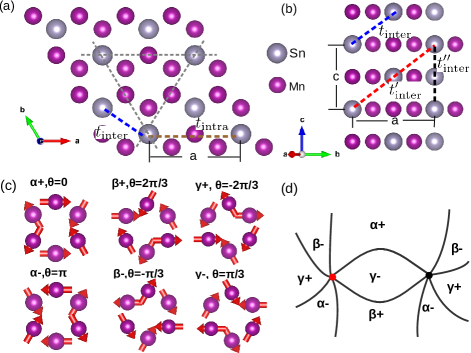
Figure 1: (a) The Lattice structure of Mn₃Sn from a top view, and (b) a side view. The thick dashed lines with brown, red, and blue colors indicate different hopping processes of the tight-binding model introduced in the text. The gray dashed lines in (a) indicate the easy axes. (c) The six magnetic domains. (d) Schematic illustration of the $\mathbb{Z}_{6}$ vortex lines.

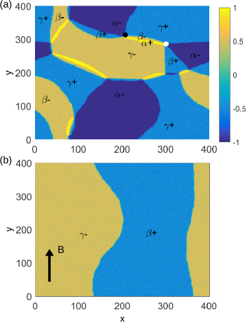
Figure 2: The spin configurations on the coarse-grained lattice at time $t=9600$ obtained from numerical simulations of the Langevin equation: (a)without any magnetic field, and (b) an external magnetic field $B=0.005\,T$ is applied along the $y$ direction.

To observe the microstructure predicted by the Langevin model, we carried out a numerical simulation of a thin slab, assuming homogeneity in the $z$ direction and discretizing the 2D continuum model with an effective lattice constant of $a_{\textrm{cg}}\!=\!600\mbox{\AA}$ – see Method section for details. Figure  2(a) shows the spin configuration resulting from a quench from a random initial state of a 576 $\mu\textrm{m}^{2}$ sample in zero applied field at an intermediate stage of evolution. Clearly there are six types of domains in the figure, marked by $\alpha^{\pm}$, $\beta^{\pm}$, and $\gamma^{\pm}$. These sixfold domains merge at the vortices and antivortices marked by white and black dots respectively.

In Fig. 2(b), we show the spin configuration resulting from the same preparation but with an applied magnetic field of $B\!=\!0.005\,\textrm{T}$ along the [120] axis ($y$ axis). As is clearly shown in the figure, the field preferentially selects just two degenerate $\beta^{+}$ ($\cos{\theta}\!=\!-1/2$) and $\gamma^{-}$ ($\cos{\theta}\!=\!1/2$) domains. The orientation of the domain wall, which tends to be normal to the [100] direction, is fixed by the anisotropic stiffness term. We will show that the double-domain pattern leads to a variety of new physics including domain-wall bound states, novel transport behavior, and domain-wall dynamics.

Minimal electronic model and electronic structure: While the ab initio electronic structure of Mn₃Sn and Mn₃Ge have been studied extensively, to study electronic properties of magnetic textures with large-scale spatial variations and/or surface/domain wall states is impractical with density functional theory. Therefore we introduce a minimal four-band tight-binding (TB) model with a single spinor ($p_{z}$) orbitals at each Sn. As indicated by the thick dashed lines in Fig. 1(a)-(b), we consider the following four hopping processes:

$$t_{\textrm{intra}}(\mathbf{r}_{nm})=t_{0}\,\mathbb{I}_{2\times 2}+t_{J}\,\mathbf{\sigma}\cdot\mathbf{S}_{nm}+(-1)^{\xi_{mn}}i\lambda_{z}\,\sigma_{z}\;,$$ (3)

$$t_{\textrm{inter}}(\mathbf{r}_{nm})=t_{1}\,\mathbb{I}_{2\times 2}\;,$$ (4)

$$t^{\prime}_{\textrm{inter}}(\mathbf{r}_{nm})=i\lambda_{\textrm{R}}\,\mathbf{e}_{\textrm{soc}}^{\mathbf{r}_{nm}}\cdot\mathbf{\sigma}\;,$$ (5)

$$t^{\prime\prime}_{\textrm{inter}}(\mathbf{r}_{nm})=t_{2}\,\mathbb{I}_{2\times 2}\;,$$ (6)

where the hopping from orbital $m$ centered at $\mathbf{r}_{m}$ to orbtial $n$ centered at $\mathbf{r}_{n}$ is expressed as a $2\times 2$ matrix due to the spin degrees freedom of each orbital, and $\mathbf{r}_{nm}\!=\!\mathbf{r}_{n}-\mathbf{r}_{m}$. The model includes three spin-independent hopping terms ($t_{0}$ in-layer and $t_{1}$ and $t_{2}$ inter-layer), a spin-dependent hopping $t_{J}$ reflecting exchange coupling to the Mn moment ${\bm{S}}$ in the middle of the bond across which the electrons hop, and two spin-orbit coupling (SOC) terms $\lambda_{z}$ and $\lambda_{R}$, which are important due to the heavy nature of the Sn ions. Details on the $\xi_{mn}$ and $\mathbf{e}_{\textrm{soc}}^{\mathbf{r}_{nm}}$ parameters which define the SOC are given in the Supp. Info. Hereafter we fix the parameters of the model as: $t_{0}\!=\!1$, $t_{1}\!=\!0.5$, $t_{J}\!=\!-0.5$, $\lambda_{z}\!=\!0.5$, $t_{2}\!=\!-1$, and $\lambda_{\textrm{R}}\!=\!0.2$. We arrange ${\bm{S}}_{nm}$ spins to reflect the spin order under consideration. In the ordered state we take the spin canting angle $\sim 1.7^{\circ}$, corresponding to a net moment $\sim 5\%$ of each Mn spin for each Kagome cell.

The bulk bandstructure of the TB model introduced above in the $\alpha^{+}$ domain is shown in Fig. 3(a). We find that in the $\alpha^{+}$ domain (see Fig. 1(c)), there are four Weyl nodes at $(\pm 0.3522,0,0)$ and $(\mp 0.3522,\pm 0.3522,0)$ at energy $E_{W1}\!=\!-2.395t_{0}$, which are denoted by solid blue dots in the inset of Fig. 3(a), with the sign corresponding to the chiralities of the Weyl nodes. There are two additional band touching points with quadratic dispersions along the $k_{z}$ direction at $(0,\pm 0.3564,0)$ at energy $E_{W2}\!=\!-2.480t_{0}$. Since the dispersion is quadratic along $k_{z}$, these two additional nodes carry zero Berry flux, and do not make significant contributions to the transport properties. The positions of the Weyl nodes in the other five domains can be obtained by applying $C_{3z}$ and/or $\mathcal{T}$ operations to those of the $\alpha^{+}$ domain.

Figure 3: (a) The bulk bandstructure of the tight-binding model in the $\alpha^{+}$ domain with $1.7^{\circ}$ spin canting. The inset indicates the positions of two different types of bulk Weyl nodes $W_{1}$ and $W_{2}$ in the $k_{z}\!=\!0$ plane. (b) The anomalous Hall conductivity $\sigma_{yz}$ in the $\alpha^{+}$ domain.

From magnetic structure to electronic properties: The most interesting feature of Mn₃Sn and its relatives is the strong influence of the magnetism on the electronic structure, and the ability to control the latter by modifying the former. The most basic electronic property is the conductivity. In the Mn₃Sn family, a symmetry analysis using crystal symmetries and Onsager relations tightly constrains the conductivity tensor (see Sec. I.4). In general the antisymmetric part of the Hall conductivity is expressed in terms of a “Hall vector” ${\bm{Q}}$, with $\frac{1}{2}(\sigma_{\mu\nu}-\sigma_{\nu\mu})=\frac{e^{2}}{2\pi h}\epsilon_{\mu\nu\lambda}Q_{\lambda}$. We evaluate ${\bm{Q}}$ in a series up to third order in the order parameter $\psi$, and express the result in terms of $\hat{\bm{K}}$, which yields

$${\bm{Q}}=q|\psi|\hat{\bm{K}}+\tilde{q}|\psi|^{3}{\rm Im}\left[(\hat{K}_{x}+i\hat{K}_{y})^{3}\right]\hat{\bm{z}}.$$ (7)

where $q|\psi|$ and $\tilde{q}|\psi|^{3}$ are parameters arising from microscopic modeling (see below). Since we expect the $O(|\psi|^{3})$ terms to be small, we observe that the Hall vector is directed along $\hat{\bm{K}}$, and lies in the xy plane. Note that, in a Weyl semimetal with all Weyl nodes at the Fermi level, ${\bm{Q}}$ is given by the fictitious dipole moment in momentum space of the Weyl points. While Mn₃Sn is a metal and this relation is not quantitively accurate, comparison of the Weyl nodes in the inset of Fig. 3(a) shows that it is qualitatively correct. We remark that due to the proportionality between the Hall vector and magnetization, ${\hat{\bm{K}}}$ can be replaced with ${\bm{M}}$ in Eq. (7), with a suitable redefinition of $q$.

To verify these symmetry considerations, we carried out a direct calculation of the full bulk conductivity tensor of the microscopic model using the Kubo formula (see Supplementary Information). We show the calculated anomalous Hall conductivity $\sigma_{zx}$ in the $\alpha^{+}$ domain in Fig. 3(b). The result is generically non-zero, but highly dependent upon the Fermi energy (the horizontal axis).

Electronic transport, electronic structure, and bound states: The direct connection of the conductivity to the order parameter suggests that transport can be a fruitful probe of magnetic microstructures. When the electronic mean free path is shorter than the length scales of magnetic textures, a local conductivity approximation is adequate: ${\bm{J}}({\bm{r}})\!=\!\underline{\sigma}[{\bm{K}}({\bm{r}})]{\bm{E}}({\bm{r}})$. From this relation and Eq. (7), the electrostatic potential can be determined for an arbitrary texture $\theta(\mathbf{r})$ (see Supp. Info.), and through inversion, it should be possible to image the magnetic domain structure purely through a spatially-resolved electrostatic measurement.

In the full quantum treatment, the electronic structure is non-trivially modified by magnetic textures. The new feature here is the appearance of Fermi arcs at domain walls. This is because a domain wall acts as a sort of internal surface, at which Fermi arc states carry chiral currents, similar to ordinary surfaces. Without loss of generality consider a minimal energy domain wall between the $\beta^{+}$ and $\gamma^{-}$ domains, which have ${\bm{K}}$ at $\pm 30^{\circ}$ from the $y$ axis. The domains have Weyl points in the $k_{z}\!=\!0$ plane, with chiralities that differ in the two domains. Distinct electronic properties thus occur when this domain wall is in an $xy$, $xz$ or $yz$ plane of the crystal.

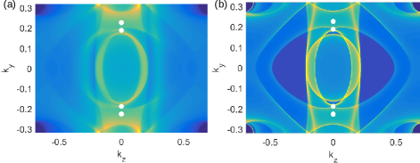
Figure 4: (a) The surface Fermi arcs of the $\beta^{+}$ domain with the surface normal vector $\hat{x}$. (b) The domain-wall Fermi arcs with the domain wall in the $yz$ plane. The white dots indicate the projection of Weyl nodes into the folded surface Brillouin zone.

Fig. 4(a) shows the surface spectral functions of the $\beta^{+}$ domain for a [100] surface. There are three Fermi arcs connecting the two projected Weyl nodes which are closer to the origin. Fig. 4(c) shows the spectral function at the interface of the $\beta^{+}$ and $\gamma^{-}$ domains with the same orientation. It shows double the Fermi arcs found at the interface, i.e. 6 instead of 3! Note that some of the projected Weyl nodes are buried in the bulk continuum due to the presence of additional Fermi surfaces around the Weyl nodes, which causes some of the Fermi arcs to merge into the bulk states before connected to the Weyl nodes. Similarly, there are also Fermi-arc states bound to the domain walls in the $xy$ and $zx$ planes (see Supp. Info.).

Short of a challenging measurement of the momentum-resolved density of states at a domain wall, how might one detect the presence of these Fermi arcs and associated bound states? We make two proposals. First, the in-plane transport within a domain wall may exhibit its own anomalous Hall effect. We checked that this indeed occurs for a $\beta^{+}-\gamma^{-}$ wall with $zx$-orientation, by calculating $\sigma_{zx}$ for a supercell with two domain walls spread over 30 primitive cells. We find $\sigma_{zx}\!=\!0.044$ for the supercell, about two times larger than the bulk value of $0.023$ found for the same cell with a uniform $\beta^{+}$ and $\gamma^{-}$ state and no domain walls. This enhancement is expected whenever $\hat{\bm{K}}$ is normal to the wall in its interior. Second, domain wall bound states can manifest as an intrinsic resistance across the wall, since they take away from the weight of continuum states which are strongly transmitted and hence contribute to conductance. We verified such a decreased conductance normal to the wall for all domain wall orientations in numerical studies (see Supp. Info.)

While we focused on the domain walls, it is worth noting that the $\mathbb{Z}_{6}$ vortex lines may have their own electronic states. Calculations in the Supp. Info. show that these vortex lines show a pronounced 6-fold pattern in their local density states, making them detectable by scanning tunnelling microscopy Tersoff and Hamann (1985).

Current-driven domain-wall dynamics Let us now consider the feedback of the conduction electrons on the spin texture. This is important to control of the magnetic microstructure electronically. In ferromagnets, current-induced forces on domains and domain walls have been extensively studied, through the mechanism of spin-transfer torqueRalph and Stiles (2008). Given that the primary order parameter of the antiferromagnet is not the magnetization, it is unclear how consideration of torque, i.e. conservation of angular momentum, applies here.

Instead, we take a symmetry-based approach and ask how the current ${\bm{j}}$ may appear as a force in the equation of motion for the easy spin angle $\theta$, Eq. (2). The result (see Supplementary Information) is that the force takes the form

$$f({\bm{j}})=-\sum_{a}\Big{(}p_{a}j_{a}\partial_{a}\theta+q_{1}{\bm{j}}\cdot\partial_{z}\hat{\bm{K}}+q_{2}j_{z}{\bm{\nabla}}\cdot\hat{\bm{K}}\Big{)}.$$ (8)

Here $p_{x}=p_{y}$, $p_{z}$, $q_{1}$ and $q_{2}$ are constants. Various arguments (see Supp. Info) suggest that $q_{1}$ and $q_{2}$, which tend to drive the domain wall along the direction perpendicular to the current flow, are much smaller than $p_{a}$, so we henceforth neglect them.

Despite the intrinsic antiferromagnetic nature of the system, the $p_{\mu}$ terms appear formally very similar to spin-transfer torques. They could be understood in a hydrodynamic fashion as describing “convection” of the spin texture with or against the current flow: indeed added to Eq. (2) , these terms are equivalent to a Galilean boost and consequently velocity $v_{a}=\mu p_{a}j_{a}$. This leads to concrete experimental proposals. Specifically, in the geometry of Fig. 2(b), a current applied along the $x$ direction controls the position of the wall. The non-dissipative Hall voltage measured between two contacts across the $y$ direction at fixed $x$ can thereby be switched by purely electrical means, as the domain wall moves to the left or right of the contacts.

The results of this paper provide the framework to design and model the spin dynamics and topologically-influenced electrical transport in the negative vector chirality antiferromagnets Mn₃Sn and Mn₃Ge, and the methodology may be applied more broadly to XY-like antiferromagnetic systems. Weyl nodes in the electronic structure induce Fermi arc bound states that influence transport in the presence of domain walls. In addition to advancing the fundamental physics of Weyl fermions in noncollinear antiferromagnets, these results mark the Mn₃Sn-class of materials as promising candidates for novel magnetic storage devices.

I Methods

I.1 Derivation of the sine-Gordon model

In this section, we present a derivation of the continuum sine-Gordon energy from a microscopic spin Hamiltonian. We consider the following spin interactions

$$H_{\textrm{s}}= J_{1}\sum_{\langle ij\rangle_{xy}}\mathbf{S}_{i}\cdot\mathbf{S}_{j}+J_{2}\sum_{\langle ij\rangle_{z}}\mathbf{S}_{i}\cdot\mathbf{S}_{j}$$

$$+\sum_{\langle ij\rangle_{xy}}\mathbf{D}_{ij}\cdot\mathbf{S}_{i}\times\mathbf{S}_{j}-\sum_{i}K\left(\hat{\mathbf{n}}_{i}\cdot\mathbf{S}_{i}\right)^{2}.$$ (9)

Here we indicated a sum over nearest-neighbors in the $xy$ plane by $\langle ij\rangle_{xy}$ and similarly nearest-neighbors in successive $xy$ planes by $\langle ij\rangle_{z}$. The spin $\mathbf{S}_{i}$ is considered as a classical vector with fixed length $m_{s}$. The positive constants $J_{1},J_{2}$ are isotropic Heisenberg interactions on these bonds. We include a Dzyaloshinskii-Moriya interaction specified by the D-vector $\mathbf{D}_{ij}=-\mathbf{D}_{ji}$ which takes the form allowed by the symmetry of the kagomé lattice. Specifically, if we choose $i$ and $j$ for a given bond so that $i\rightarrow j$ proceeds counter-clockwise on the triangle to which the bond belongs, then we have

$$\mathbf{D}_{ij}=D\hat{\mathbf{z}}+D^{\prime}\hat{\mathbf{z}}\times\hat{\mathbf{e}}_{ij},$$ (10)

where $\hat{\mathbf{e}}_{ij}$ is the unit vector oriented from site $i$ to site $j$. It worth to note that prior modeling of the spin interactions in Mn₃Sn have included the $D$ term but not the $D^{\prime}$ one. The $K$ term is a local easy-axis anisotropy, which is determined by the unit vector $\hat{\mathbf{n}}_{i}$ oriented along the direction between the spin $i$ and either of its nearest Sb ions as indicated by the gray dashed line in Fig. 1(a).

We first assume a uniform spin configuration, which is sufficient to describe the ground state, and it determines the $Z_{6}$ anisotropy $\lambda$. There are six spins per unit cell, which form two triangles, one in each of the two distinct layers. By inspection, we find that there is inversion symmetry in the magnetic ground state and we only have to consider the spins in one triangle. The Heisenberg term in Eq. (I.1) is minimized by requiring the three spins to lie in a plane at 120 degree angles to one another. The plane of the spins is undetermined by the Heisenberg term, but fixed by the DM interaction. To leading order in the DM terms, the ground state is of the form

$$\mathbf{S}^{(0)}_{a}=m_{s}\begin{pmatrix}\cos(-\theta-\tfrac{2\pi a}{3})\\ \sin(-\theta-\tfrac{2\pi a}{3})\\ 0\end{pmatrix}.$$ (11)

We also include small “canting” of the spins away from the rigid configuration. Formally, we do this by writing $K\rightarrow\eta K$, $D\rightarrow\eta D$, $D^{\prime}\rightarrow\eta D^{\prime}$, and carrying out perturbation theory in $\eta$. To do so, we let

$$\mathbf{S}_{a}=m_{s}\begin{pmatrix}\sqrt{1-u_{a}^{2}}\cos(-\theta-\tfrac{2\pi a}{3}+\phi_{a})\\ \sqrt{1-u_{a}^{2}}\sin(-\theta-\tfrac{2\pi a}{3}+\phi_{a})\\ u_{a}\end{pmatrix},$$ (12)

where $a=1,2,3$ denote the sublattice indices of the kagomeĺattice. We set $\phi_{3}=-\phi_{1}-\phi_{2}$ to keep $\phi_{1},\phi_{2}$ linearly independent of $\theta$. We also write $u_{1,2,3}$ and $\phi_{1,2}$ in a series in $\eta$, $u_{a}=\sum_{n=1}^{\infty}u_{a,n}\eta^{n}$, $\phi_{a}=\sum_{n=1}^{\infty}\phi_{a,n}\eta^{n}.$ Inserting Eq. (12) into the spin Hamiltonian , we then obtain a formal expansion of the energy order by order in $\eta$. Keeping the expansion to the third order in $\eta$, then minimizing with respect to $u_{a}$ and $\phi_{a}$, we obtain the optimal spin configuration to first order in the canting angles, and the ground state energy to third order in $\eta$:

$$E_{\textrm{gs}}=\mathcal{E}_{0}-\frac{K^{3}}{12(J_{1}+J_{2})^{2}}m_{s}^{2}\cos 6\theta,$$ (13)

where $\mathcal{E}_{0}$ is a $\theta$-independent constant. The coefficient of $\cos 6\theta$ in Eq. (13) allows us to determine $\lambda$ in the sine-Gordon model.

Further results are obtained by adding the effect of a Zeeman magnetic field to the energy. We repeat the previous analysis, taking the magnetic field $\mathbf{B}\rightarrow\eta\mathbf{B}$ as well. This corresponds to considering the Zeeman energy much small than $J_{1}+J_{2}$, an excellent approximation. It turns out that the leading term in the in-plane magnetization is

$$\mathbf{M}_{xy}=\frac{Kgm_{s}}{J_{1}+J_{2}}\begin{pmatrix}\cos\theta\\ \sin\theta\\ 0\end{pmatrix}\equiv\frac{Kgm_{s}}{J_{1}+J_{2}}\hat{\mathbf{K}},$$ (14)

One may note that the angle of the net magnetization $\theta$ is minus the $U(1)$ rotation angle , which is due to the antichiral spin texture on kagomeĺattice. We refer the readers to Supp. Info. for more details.

The out-of-plane magnetization turns out to be parametrically smaller by a factor of $D^{\prime}/J$:

$$M_{z}=-\frac{D^{\prime}Kgm_{s}}{\sqrt{3}(J_{1}+J_{2})^{2}}\sin 3\theta.$$ (15)

The above equation shows that the magnetization does not stay entirely within the $xy$ plane. For $\lambda>0$, where the minimum energy values of $\theta$ are multiples of $2\pi/6$, then $\sin 3\theta=0$ and the bulk $z$-axis magnetization within a uniform domain vanishes. This corresponds to the case in which one of the three spins on each triangle orients along its easy axis, directly toward a neighboring Sn. One can verify that this situation preserves a mirror plane which enforces $M^{z}=0$. For $\lambda<0$, however, $\sin 3\theta=\pm 1$ at the minimum values of $\theta$, and so the domains are expected to have a small bulk magnetization, reduced by a factor of $D^{\prime}/\sqrt{3}(J_{1}+J_{2})$ relative to the in-plane magnetization. Since such a $z$-axis magnetization seems not to have been detected in Mn₃Sn, we take this as evidence in favor of the $\lambda>0$ state. Even for this state, however, we see that the out of plane magnetization $M^{z}$ becomes non-zero within domain walls. We remark in passing that experiments show that in Mn₃Ge the anomalous Hall conductivity within the $xy$ plane is small but nonvanishingNayak et al. (2016), suggesting that the $\lambda>0$ state is realized in Mn₃Ge.

We continue to study the magnetic susceptibilities in the high-field regime, i.e., when the spontaneous magnetization is much smaller than the field-induced one. When the field is within the $xy$ plane, $\mathbf{B}=B(\cos{\alpha},\sin{\alpha},0)$, the in-plane susceptibility is expressed as

$$\chi_{\perp c}\!=\!\chi_{\perp c,0}+\chi_{\perp c,1}\cos{6\alpha},$$ (16)

where

$$\chi_{\perp c,0} = \frac{g^{2}}{J_{1}+J_{2}}\Big{(}\,1-\frac{\sqrt{3}D}{J_{1}+J_{2}}\,\Big{)}\;,$$ (17)

$$\chi_{\perp c,1} = \frac{Kg^{2}}{6(J_{1}+J_{2})^{2}}.$$ (18)

It follows that the in-plane magnetization is linear in field with an offset $M_{xy}$ (see Eq. (14)), and a six-fold modulation. Measurement of the six-fold modulation provides a way to determine $K/(J_{1}+J_{2})$.

On the other hand, when the magnetic field is along the $z$ direction, the out-of-plane susceptibility is expressed as

$$\chi_{\parallel c}=\frac{g^{2}}{J_{1}+J_{2}}\Big{(}\,1-\frac{\sqrt{3}D}{3(J_{1}+J_{2})}\,\Big{)}\;.$$ (19)

The exchange $J_{1}+J_{2}$ and DM parameter $D$ can be determined by susceptibility measurements using Eq. (18) and (19).

To obtain the full continuum theory, we need to allow slow spatial variations of $\theta$. To do so, we introduce the parametrization similar to Eq. (12) but with no assumptions about uniformity or symmetry:

$$\mathbf{S}_{a,s}(\mathbf{r})=m_{s}\begin{pmatrix}\sqrt{1-u_{a,s}^{2}(\mathbf{r})}\cos(-\theta(\mathbf{r})-\tfrac{2\pi a}{3}+\phi_{a,s}(\mathbf{r}))\\ \sqrt{1-u_{a,s}^{2}(\mathbf{r})}\sin(-\theta(\mathbf{r})-\tfrac{2\pi a}{3}+\phi_{a,s}(\mathbf{r}))\\ u_{a,s}(\mathbf{r}).\end{pmatrix}$$ (20)

The idea now is to insert the ansatz in Eq. (20) into the spin Hamiltonian, and expand both in powers of $\phi_{a,s}$ and $u_{a,s}$ and in gradients. The leading stiffness terms can be obtained by minimizing the spin Hamiltonian with respect to $\phi_{a,s}$ and $u_{a,s}$ at fixed $\theta$. The result is

$$H =\sum_{\mathbf{r}} \Big{[}\frac{9m_{s}^{2}a_{0}^{2}J_{1}(3J_{1}+2J_{2})}{2(3J_{1}+J_{2})}\left(|\partial_{x}\theta|^{2}+|\partial_{y}\theta|^{2}\right)$$ (21)

$$+12d^{2}m_{s}^{2}J_{2}|\partial_{z}\theta|^{2}\Big{]}.$$

From this the stiffnesses can be read off.

The only remaining term in the continuum energy to be discussed is anisotropic gradient one. For simplicity, we neglect the possible effect of the DM interactions on this term, and set $D=D^{\prime}=0$. We anticipate that the anisotropic stiffness appears with a coefficient of order $K$. We treat the gradients, small canting angle, and $K$, all of the same order, and expand the energy up to $O(\phi^{3})$. Due to the lack of mixing between $z$ and $xy$ components when $D^{\prime}=0$, the out of plane canting components $u_{a,s}$ have no effect and we can set them to zero. Then one may minimize the energy with respect to $\phi_{a}$, and select the terms second order in gradients. After carrying through this algebra, we obtain

$$H^{(3)}=\rho_{1}\sum_{\mathbf{r}}\Big{[}(\hat{\mathbf{K}}\cdot\mathbf{\nabla}\theta)^{2}-\tfrac{1}{2}|\mathbf{\nabla}_{\perp}\theta|^{2}\Big{]},$$ (22)

with $\hat{\mathbf{K}}=(\cos\theta,\sin\theta,0)$ and

$$\rho_{1}=\frac{15m_{s}^{2}a_{0}^{2}KJ_{1}(9J_{1}^{2}+3J_{1}J_{2}+2J_{2}^{2})}{2(J_{1}+J_{2})(3J_{1}+J_{2})^{2}}.$$ (23)

We refer the readers to Supp. Info. for more details about the derivation of the continuum theory.

I.2 Evaluations of the sine-Gordon parameters

As discussed above, the exchange interaction $J_{1}+J_{2}$ and DM interaction $D$ can be determined by the susceptibility measurements using Eq. (17) and (19). We have used the data measured at $300$ K as reported in Ref. Nakatsuji et al., 2015, and find that $J_{1}+J_{2}=5.606$ meV, and $D=0.635\,$meV. The ratio $K/(J_{1}+J_{2})$ can be determined by measuring the six-fold modulations of the in-plane magnetizations . It turns out that $K=0.187$ meV. The finite-temperature effect is taken into account by letting $m_{s}\to m_{s}(T)$, where $m_{s}(T)$ is the mean-field expectation value of a spin $1$ at temperature $T$. In particular, at $T=50$ K, $m_{s}(T)=0.92$. Given the specific values of $J_{1}+J_{2}$, $D$, $K$ and $m_{s}(T)$, we evaluate the $\mathbb{Z}_{6}$ anisotropy $\lambda=1.159\times 10^{-7}$ meV/$\mbox{\AA}^{-3}$, the isotropic stiffness $\rho=0.568$ meV/Å, and the anisotropic stiffness $\rho_{1}=0.011$ meV/Å. We may also obtain the canting moment from Eq. (14), which turns out to be 0.061 $\mu_{\textrm{B}}$ per unit cell at 50 K, from which we obtain the Zeeman energy density for in-plane magnetic field $B$ as $h=M_{xy}B=2.814\times 10^{-3}B$ meV$\mbox{\AA}^{-3}$T^-1, where $B$ is the magnitude of the magnetic field in units of Tesla. Note that the estimated canting moment is about 5 times larger than the experimental measurements, and we suspect that the measured value has underestimated the canting moment due to the cancellation from different domains.

I.3 Domain-wall bound states

The surface spectral functions as shown in Fig. 4(a) are calculated using the method proposed in Ref. Sancho et al., 1985. In order to calculate the domain-wall spectral functions, we include the domain-wall layers coupled to the two semi-infinite domains, and the thickness of the domain wall is $N_{\textrm{dw}}$ (in units of lattice constants). The spins vary smoothly from one domain to the other across the domain wall. The domain-wall spectral function can be solved using the Dyson equation,

$$G_{\textrm{dw}}=G_{\textrm{dw}}^{0}+G_{\textrm{dw}}^{0}(\mathbf{k},\omega)\Sigma_{\textrm{dw}}G_{\textrm{dw}}\;,$$ (24)

where $G_{\textrm{dw}}$ represents the retarded Green’s function of the domain wall including the effects due to the couplings to two domains, while $G_{\textrm{dw}}^{0}$ is the “bare” Green’s function excluding the coupling between the domain wall and the domains, and $\Sigma_{\textrm{dw}}$ is the self energy from the coupling. In the above equation the dependence on the 2D wavevector $\mathbf{k}$ and the frequency $\omega$ is implicit. More specifically,

$$G_{\textrm{dw}}^{0}=\begin{pmatrix}G_{\beta^{+}}^{s}&0&0\\ 0&G_{00}&0\\ 0&0&G_{\gamma^{-}}^{s}\end{pmatrix}\;,$$ (25)

where $G_{00}$ is the Green’s function of the isolated domain-wall layers, and $G_{\beta^{+}}^{s}$ and $G_{\gamma^{-}}^{s}$ denote the surface Green’s functions of the $\beta^{+}$ and $\gamma^{-}$ domains calculated using the iterative scheme proposed in Ref. Sancho et al., 1985. The self energy $\Sigma_{\textrm{dw}}$ is simply the coupling between the domain wall and the domains,

$$\Sigma_{\textrm{dw}}=\begin{pmatrix}0&H_{\beta^{+},\textrm{dw}}&0\\ H_{\beta^{+},\textrm{dw}}^{\dagger}&0&H_{\textrm{dw},\gamma^{-}}\\ 0&H^{\dagger}_{\textrm{dw},\gamma^{-}}&0\;.\end{pmatrix}$$ (26)

I.4 Symmetry analysis on the conductivity tensor

In this section we derive the symmetry-allowed expressions of the bulk conductivity tensor. We consider four generators of the symmetry operations of space group $P6_{3}/mmc$: $120^{\circ}$ rotation about $z$ axis $C_{3z}$, $180^{\circ}$ rotation about an in-plane axis which is parallel to [100] and half-way between the $z\!=\!0$ and $z\!=\!c/2$ plane $C_{2x}$, a $180^{\circ}$ screw rotation about $z$ axis $C_{2z}^{s}$, and finally inversion $\mathcal{P}$. The full conductivity tensor $\underline{\sigma}$ can be expressed as:

$$\underline{\sigma}= \underline{\sigma}^{0}+\sum_{\mu=x,y}\underline{A}^{\mu}|\psi|\hat{K}_{\mu}+\sum_{\mu,\nu}\underline{B}^{\mu\nu}|\psi|^{2}\hat{K}_{\mu}\hat{K}_{\nu}+\mathcal{O}(|\psi|^{3})\;,$$ (27)

where $K_{\mu}$ is the $\mu$th component of the order parameter $\mathbf{\hat{K}}=(\cos\theta,\sin\theta,0)$. $\underline{\sigma}^{0}$ is the term which is independent of magnetic state, while $\underline{A}^{\mu}$ and $\underline{B}^{\mu\nu}$ couples to $\mathbf{\hat{K}}$ to the linear and quadratic orders respectively. Due to Onsager reciprocal relation, the terms which are odd (even) in $\hat{K}_{\mu}$ have to be antisymmetric (symmetric). Thus $\underline{A}^{\mu}$ is antisymmetric, while $\underline{\sigma}^{0}$ and $\underline{B}^{\mu\nu}$ are symmetric.

Table 1: Symmetry representations

$g$	$\Gamma_{g}$	$\mathcal{O}_{g}$
$C_{3z}$	$\begin{pmatrix}-\frac{1}{2}&-\frac{\sqrt{3}}{2}\\ \frac{\sqrt{3}}{2}&-\frac{1}{2}\end{pmatrix}$	$\begin{pmatrix}-\frac{1}{2}&-\frac{\sqrt{3}}{2}&0\\ \frac{\sqrt{3}}{2}&-\frac{1}{2}&0\\ 0&0&1\end{pmatrix}$
$C_{2x}$	$\begin{pmatrix}1&0\\ 0&-1\end{pmatrix}$	$\begin{pmatrix}1&0&0\\ 0&-1&0\\ 0&0&-1\end{pmatrix}$
$C_{2z}^{s}$	$\begin{pmatrix}-1&0\\ 0&-1\end{pmatrix}$	$\begin{pmatrix}-1&0&0\\ 0&-1&0\\ 0&0&1\end{pmatrix}$
$\mathcal{P}$	$\begin{pmatrix}1&0\\ 0&1\end{pmatrix}$	$\begin{pmatrix}-1&0&0\\ 0&-1&0\\ 0&0&-1\end{pmatrix}$

The conductivity tensor should be invariant under a symmetry operation $g$, which means

$$\mathcal{O}_{g}\,\underline{\sigma}^{0}\,\mathcal{O}_{g}^{T}=\underline{\sigma}^{0}\;$$

$$\mathcal{O}_{g}\,\underline{A}^{\mu}\,\mathcal{O}_{g}^{T}=\sum_{\mu=x,y}\Gamma_{g,\mu\nu}\,\underline{A}^{\nu}\;$$

$$\mathcal{O}_{g}\,\underline{B}^{\mu\nu}\,\mathcal{O}_{g}^{T}=\sum_{\mu^{\prime},\nu^{\prime}}\Gamma_{g,\mu\mu^{\prime}}\Gamma_{g,\nu\nu^{\prime}}\,\underline{B}^{\mu^{\prime}\nu^{\prime}}\;,$$ (28)

where $\mathcal{O}_{g}$ is a $3\times 3$ matrix representing the symmetry operation $g$ on a 3D real vector, and $\Gamma_{g}$ is a $2\times 2$ matrix representing the symmetry operation $g$ acting on the $xy$ component of $\mathbf{\hat{K}}$. The symmetry representations $\mathcal{O}_{g}$ and $\Gamma_{g}$ are tabulated in Table 1. After solving Eq. (28), we obtain the symmetry-allowed conductivity tensor:

$$\sigma_{\mu\nu}=\sigma_{\parallel}\delta_{\mu\nu}+(\sigma_{\perp}-\sigma_{\parallel})\delta_{\mu z}\delta_{\nu z}+q|\psi|\epsilon_{\mu\nu\lambda}\hat{K}_{\lambda}+b_{1}|\psi|^{2}\hat{K}_{\mu}\hat{K}_{\nu}\;,$$ (29)

where $\sigma_{\perp}$ denotes the out-of-plane diagonal conductivity, $\sigma_{\parallel}$ denotes the isotropic part of the in-plane diagonal conductivity, $b_{1}$ denotes the anisotropic part of the in-plane conductivity, and finally $q$ term denotes the anomalous Hall conductivity. We refer the readers to Supp. Info. for more details about the numerical calculations of the conductivities.

I.5 Symmetry analysis on the spin-transfer torques

In this section we provide a derivation of Eq. (8). The general expression for the current-induced spin-transfer torque is:

$$f(\mathbf{j})=-\sum_{a,b}(B_{0}^{ab}\,j_{a}\,\partial_{b}\theta+B_{1}^{ab}\,j_{a}\,\partial_{b}\theta\cos{\theta}+B_{2}^{ab}\,j_{a}\,\partial_{b}\theta\sin{\theta})\;,$$ (30)

where $j_{a}$ denotes the $a$ component of the electric current with $a,b\!=\!x,y,z$. The dependence of $\theta$ on position and time is implicit. It is convenient to decompose Eq. (30) as $f(\mathbf{j})=f_{p}(\mathbf{j})+f_{q}(\mathbf{j})$, where the leading term $f_{p}(\mathbf{j})=-\sum_{a,b}B_{0}^{ab}j_{a}\partial_{b}\theta$, and the subleading term $f_{q}(\mathbf{j})=-\sum_{a,b}(B_{1}^{ab}\,j_{a}\,\partial_{b}\theta\cos{\theta}+B_{2}^{ab}\,j_{a}\,\partial_{b}\theta\sin{\theta})$.

Let us first consider the $f_{p}(\mathbf{j})$ term. The $U(1)$ rotation $\theta$ is transformed to $\theta_{g}$ after a symmetry operation $g$. More specifically,

$$C_{3z}:\hskip 6.0pt\theta\to\theta_{g}=\theta+\frac{2\pi}{3}\;,$$

$$C_{2x}:\hskip 6.0pt\theta\to\theta_{g}=-\theta\;,$$

$$C_{2z}^{s}:\hskip 6.0pt\theta\to\theta_{g}=\theta+\pi\;,$$

$$\mathcal{P}:\hskip 6.0pt\theta\to\theta_{g}=\theta\;.$$ (31)

With a symmetry operation $g$, the spin-transfer torque $f_{p}(\mathbf{j})\!\to\!f_{p,g}(\mathbf{j})$, where

$$f_{p,g}(\mathbf{j}) =-\sum_{a,a^{\prime},b,b^{\prime}}\,B_{0}^{ab}\,\mathcal{O}_{g,a^{\prime}a}^{T}\,\mathcal{O}_{g,bb^{\prime}}\,j_{a^{\prime}}\,\partial_{b^{\prime}}\,\theta_{g}\;$$

$$=-\sum_{a,b}B_{0}^{ab}\,j_{a}\,\partial_{b}\,\theta_{g}\;.$$ (32)

It follows that

$$\sum_{a^{\prime}b^{\prime}}\,\mathcal{O}_{g,aa^{\prime}}^{T}\,B_{0}^{a^{\prime}b^{\prime}}\,\mathcal{O}_{g,b^{\prime}b}=B_{0}^{ab}\;,$$ (33)

where $\mathcal{O}_{g}$ is tabulated in Table 1. After solving Eq. (33), one obtains the $p_{a}j_{a}\partial\theta$ term in Eq. (8).

The $f_{q}(\mathbf{j})$ term is more complicated. Under a symmetry transformation $g$, $f_{q}(\mathbf{j})\to f_{q,g}(\mathbf{j})$, where

$$f_{q,g}(\mathbf{j}) =-\sum_{aa^{\prime}bb^{\prime}}\sum_{\mu=x,y}\Big{(}\,B_{1}^{ab}\,\mathcal{O}^{T}_{g,a^{\prime}a}\,\mathcal{O}_{g,bb^{\prime}}\,j_{a^{\prime}}\,\partial_{b^{\prime}}\theta_{g}\,\Gamma_{g,x\mu}\,\hat{K}_{\mu}+B_{2}^{ab}\,\mathcal{O}^{T}_{g,a^{\prime}a}\,\mathcal{O}_{g,bb^{\prime}}\,j_{a^{\prime}}\,\partial_{b^{\prime}}\theta_{g}\,\Gamma_{g,y\mu}\,\hat{K}_{\mu}\,\Big{)}\;$$

$$=-\sum_{ab}\Big{(}\,B_{1}^{ab}\,j_{a}\,\partial_{b}\theta_{g}\,\hat{K}_{x}+B_{2}^{ab}\,j_{a}\,\partial_{b}\theta_{g}\,\hat{K}_{y}\,\Big{)}\;,$$ (34)

where the matrix $\Gamma_{g}$ has been tabulated in Table 1, $\hat{K}_{x}=\cos{\theta}$, and $\hat{K}_{y}=\sin{\theta}$. From the above equation it follows that

$$\sum_{a^{\prime}b^{\prime}}\mathcal{O}_{g,aa^{\prime}}^{T}\,(\,B_{1}^{a^{\prime}b^{\prime}}\,\Gamma_{g,xx}+B_{2}^{a^{\prime}b^{\prime}}\,\Gamma_{g,yx}\,)\,\mathcal{O}_{g,b^{\prime}b}=B_{1}^{ab}\;,$$

$$\sum_{a^{\prime}b^{\prime}}\mathcal{O}_{g,aa^{\prime}}^{T}\,(\,B_{2}^{a^{\prime}b^{\prime}}\,\Gamma_{g,yy}+\,B_{1}^{a^{\prime}b^{\prime}}\,\Gamma_{g,xy}\,)\,\mathcal{O}_{g,b^{\prime}b}=B_{2}^{ab}.\;$$ (35)

One would obtain the $q_{1}$, $q_{2}$ terms in Eq. (8) after solving the above equations.

Acknowledgements: We thank the groups of Professors Satoru Nakatsuji and Yoshichika Otani for introducing us to these materials and sharing their data. This research was supported by the National Science Foundation under grant number DMR1506119.

References

- Karplus and Luttinger (1954) R. Karplus and J. M. Luttinger, Phys. Rev. 95, 1154 (1954).
- Nagaosa et al. (2010) N. Nagaosa, J. Sinova, S. Onoda, A. MacDonald, and N. Ong, Reviews of modern physics 82, 1539 (2010).
- Hasan and Kane (2010) M. Z. Hasan and C. L. Kane, Rev. Mod. Phys. 82, 3045 (2010).
- Qi and Zhang (2011) X.-L. Qi and S.-C. Zhang, Rev. Mod. Phys. 83, 1057 (2011).
- Wan et al. (2011) X. Wan, A. M. Turner, A. Vishwanath, and S. Y. Savrasov, Phys. Rev. B 83, 205101 (2011).
- Burkov et al. (2011) A. A. Burkov, M. D. Hook, and L. Balents, Phys. Rev. B 84, 235126 (2011).
- Burkov and Balents (2011) A. A. Burkov and L. Balents, Phys. Rev. Lett. 107, 127205 (2011).
- Xu et al. (2011) G. Xu, H. Weng, Z. Wang, X. Dai, and Z. Fang, Physical review letters 107, 186806 (2011).
- Murakami (2007) S. Murakami, New Journal of Physics 9, 356 (2007).
- Wang et al. (2012) Z. Wang, Y. Sun, X.-Q. Chen, C. Franchini, G. Xu, H. Weng, X. Dai, and Z. Fang, Physical Review B 85, 195320 (2012).
- Wang et al. (2013) Z. Wang, H. Weng, Q. Wu, X. Dai, and Z. Fang, Physical Review B 88, 125427 (2013).
- Turner et al. (2013) A. M. Turner, A. Vishwanath, and C. O. Head, Topological Insulators 6, 293 (2013).
- Liu and Vanderbilt (2014) J. Liu and D. Vanderbilt, Phys. Rev. B 90, 155316 (2014).
- Weng et al. (2015) H. Weng, C. Fang, Z. Fang, B. A. Bernevig, and X. Dai, Phys. Rev. X 5, 011029 (2015).
- Soluyanov et al. (2015) A. A. Soluyanov, D. Gresch, Z. Wang, Q. Wu, M. Troyer, X. Dai, and B. A. Bernevig, Nature 527, 495 (2015).
- Yang et al. (2015) L. Yang, Z. Liu, Y. Sun, H. Peng, H. Yang, T. Zhang, B. Zhou, Y. Zhang, Y. Guo, M. Rahn, et al., Nature Physics 11, 728 (2015).
- Lv et al. (2015) B. Lv, H. Weng, B. Fu, X. Wang, H. Miao, J. Ma, P. Richard, X. Huang, L. Zhao, G. Chen, et al., Physical Review X 5, 031013 (2015).
- Huang et al. (2015) S.-M. Huang, S.-Y. Xu, I. Belopolski, C.-C. Lee, G. Chang, B. Wang, N. Alidoust, G. Bian, M. Neupane, C. Zhang, et al., Nature communications 6 (2015).
- Chen et al. (2014) H. Chen, Q. Niu, and A. H. MacDonald, Phys. Rev. Lett. 112, 017205 (2014).
- Nakatsuji et al. (2015) S. Nakatsuji, N. Kiyohara, and T. Higo, Nature (2015).
- Nayak et al. (2016) A. K. Nayak, J. E. Fischer, Y. Sun, B. Yan, J. Karel, A. C. Komarek, C. Shekhar, N. Kumar, W. Schnelle, J. Kübler, et al., Science advances 2, e1501870 (2016).
- Yang et al. (2016) H. Yang, Y. Sun, Y. Zhang, W.-J. Shi, S. S. Parkin, and B. Yan, arXiv preprint arXiv:1608.03404 (2016).
- Kübler and Felser (2014) J. Kübler and C. Felser, EPL (Europhysics Letters) 108, 67001 (2014).
- Tomiyoshi and Yamaguchi (1982) S. Tomiyoshi and Y. Yamaguchi, Journal of the Physical Society of Japan 51, 2478 (1982).
- Brown et al. (1990) P. Brown, V. Nunez, F. Tasset, J. Forsyth, and P. Radhakrishna, Journal of Physics: Condensed Matter 2, 9409 (1990).
- Kren et al. (1975) E. Kren, J. Paitz, G. Zimmer, and E. Zsoldos, Physica B+ C 80, 226 (1975).
- Nagamiya et al. (1982) T. Nagamiya, S. Tomiyoshi, and Y. Yamaguchi, Solid State Communications 42, 385 (1982).
- Tersoff and Hamann (1985) J. Tersoff and D. R. Hamann, Phys. Rev. B 31, 805 (1985).
- Ralph and Stiles (2008) D. C. Ralph and M. D. Stiles, Journal of Magnetism and Magnetic Materials 320, 1190 (2008).
- Sancho et al. (1985) M. L. Sancho, J. L. Sancho, J. L. Sancho, and J. Rubio, Journal of Physics F: Metal Physics 15, 851 (1985).