Normal form of swallowtail and its applications

Abstract

We construct a form of swallowtail singularity in $\boldsymbol{R}^{3}$ which uses coordinate transformation on the source and isometry on the target. As an application, we classify configurations of asymptotic curves and characteristic curves near swallowtail.

1 Introduction

Wave fronts and frontals are surfaces in $3$-space, and they may have singularities. They always have normal directions even along singularities. Recently, there appeared several articles concerning on differential geometry of wave fronts and frontals [14, 15, 16, 17, 20, 21, 23, 24, 25]. Surfaces which have only cuspidal edges and swallowtails as singularities are the generic wave fronts in the Euclidean $3$-space. Fundamental differential geometric invariants of cuspidal edge is defined in [25]. It is further investigated in [20, 21, 18], where the normal form of cuspidal edge plays a important role. The normal form of a singular point is a parametrization using by coordinate transformation on the source and isometric transformation on the target[5, 28]. For the purpose of differential geometric investigation of singularities, it is not only convenient, but also indispensable to studying higher order invariants. Higher order invariants of cuspidal edges are studied in [23], and in [23], moduli of isometric deformations of cuspidal edge is determined. In this paper, we give a normal form of swallowtail, and study relationships to previous investigation of swallowtail. As an application, we study geometric foliations near swallowtail.

The precise definition of the swallowtail is given as follows: The unit cotangent bundle $T^{*}_{1}\boldsymbol{R}^{3}$ of $\boldsymbol{R}^{3}$ has the canonical contact structure and can be identified with the unit tangent bundle $T_{1}\boldsymbol{R}^{3}$. Let $\alpha$ denote the canonical contact form on it. A map $i:M\to T_{1}\boldsymbol{R}^{3}$ is said to be isotropic if the pull-back $i^{*}\alpha$ vanishes identically, where $M$ is a $2$-manifold. If $i$ is an immersion, then we call the image of $\pi\circ i$ the wave front set of $i$, where $\pi:T_{1}\boldsymbol{R}^{3}\to\boldsymbol{R}^{3}$ is the canonical projection and we denote it by $W(i)$. Moreover, $i$ is called the Legendrian lift of $W(i)$. With this framework, we define the notion of fronts as follows: A map-germ $f:(\boldsymbol{R}^{2},0)\to(\boldsymbol{R}^{3},0)$ is called a frontal if there exists a unit vector field (called unit normal of $f$) $\nu$ of $\boldsymbol{R}^{3}$ along $f$ such that $L=(f,\nu):(\boldsymbol{R}^{2},0)\to(T_{1}\boldsymbol{R}^{3},0)$ is an isotropic map by an identification $T_{1}\boldsymbol{R}^{3}=\boldsymbol{R}^{3}\times S^{2}$, where $S^{2}$ is the unit sphere in $\boldsymbol{R}^{3}$ (cf. [1], see also [19]). A frontal $f$ is a front if the above $L$ can be taken as an immersion. A point $q\in(\boldsymbol{R}^{2},0)$ is a singular point if $f$ is not an immersion at $q$. A map $f:M\to N$ between $2$-dimensional manifold $M$ and $3$-dimensional manifold $N$ is called a frontal (respectively, a front) if for any $p\in M$, the map-germ $f$ at $p$ is a frontal (respectively, a front). A singular point $p$ of a map $f$ is called a cuspidal edge if the map-germ $f$ at $p$ is $\mathcal{A}$-equivalent to $(u,v)\mapsto(u,v^{2},v^{3})$ at $0$, and a singular point $p$ is called a swallowtail if the map-germ $f$ at $p$ is $\mathcal{A}$-equivalent to $(u,v)\mapsto(u,4v^{3}+2uv,3v^{4}+uv^{2})$ at $0$, (Two map-germs $f_{1},f_{2}:(\boldsymbol{R}^{n},0)\to(\boldsymbol{R}^{m},0)$ are $\mathcal{A}$- equivalent if there exist diffeomorphisms $S:(\boldsymbol{R}^{n},0)\to(\boldsymbol{R}^{n},0)$ and $T:(\boldsymbol{R}^{m},0)\to(\boldsymbol{R}^{m},0)$ such that $f_{2}\circ S=T\circ f_{1}$.) Therefore if the singular point $p$ of $f$ is a swallowtail, then $f$ at $p$ is a front.

2 Singular points of $k$-th kind

Let $f:(\boldsymbol{R}^{2},0)\to(\boldsymbol{R}^{3},0)$ be a frontal and $\nu$ its unit normal. Let $\lambda$ be a function which is a non-zero functional multiplication of the function

$$\det(f_{u},f_{v},\nu)$$

for some coordinate system $(u,v)$, and $(~{})_{u}=\partial/\partial u$, $(~{})_{v}=\partial/\partial v$. We call such function singularity identifier. A singular point $p$ of $f$ is called non-degenerate if $d\lambda(p)\neq 0$. Let $0$ be a non-degenerate singular point of $f$. Then the set of singular points $S(f)$ is a regular curve, we take a parameterization $\gamma(t)$ $(\gamma(0)=0)$ of it. We set $\hat{\gamma}=f\circ\gamma$ and call $\hat{\gamma}$ singular locus. One can show that there exists a vector field $\eta$ such that if $p\in S(f)$, then

$$\ker df_{p}=\left\langle{\eta_{p}}\right\rangle_{\boldsymbol{R}}.$$

We call $\eta$ the null vector field. On $S(f)$, $\eta$ can be parameterized by the parameter $t$ of $\gamma$. We denote by $\eta(t)$ the null vector field along $\gamma$. We set

$$\varphi(t)=\det\left(\dfrac{d\gamma}{dt}(t),\eta(t)\right).$$ (2.1)

Definition 2.1.

A non-degenerate singular point $0$ is the first kind if $\varphi(0)\neq 0$. A non-degenerate singular point $0$ is the $k$-th kind ($k\geq 2$) if

$$\dfrac{d\varphi}{dt}(0)=\cdots=\dfrac{d^{k-2}\varphi}{dt^{k-2}}(0)=0,\quad\dfrac{d^{k-1}\varphi}{dt^{k-1}}(0)\neq 0.$$

The definition does not depend on the choice of the parameterization of $\gamma$ and choice of $\eta$. We remark that if $f$ is a front, then the singular point of the first kind is the cuspidal edge, and the singular point of the second kind is the swallowtail [19]. We can rephrase the definition of the $k$-th kind singularity as follows. Let $0$ be a non-degenerate singular point of $f$. Then there exists a vector field $\tilde{\eta}$ such that if $p\in S(f)$ then $\ker df_{p}=\left\langle{\eta_{p}}\right\rangle_{\boldsymbol{R}}.$ We call $\tilde{\eta}$ the extended null vector field.

Lemma 2.2.

Let $0$ be a non-degenerate singular point $0$ of a frontal $f:(\boldsymbol{R}^{2},0)\to(\boldsymbol{R}^{3},0)$, and let $\lambda$ be a singularity identifier. Then the followings are equivalent.

1. $0$ is a singular point of the $k$-th kind,

2. $\eta\lambda=\cdots=\eta^{k-1}\lambda(0)=0,\eta^{k}\lambda(0)\neq 0,$ where $\eta$ is a null vector field, and $\eta^{i}$ stands for the $i$ times directional derivative by $\eta$.

Firstly we show that the condition (2) does not depend on the choices of $\eta$ and $\lambda$. It is obvious that for the choice of $\lambda$, we shoe it for the choice of $\tilde{\eta}$. We show the following lemma.

Lemma 2.3.

Let $\lambda:(\boldsymbol{R}^{2},0)\to(\boldsymbol{R},0)$ be a function satisfying $d\lambda(0)\neq 0$, and let $\eta$ be a vector field. Let $\overline{\eta}$ be another vector field satisfying $\overline{\eta}=h\tilde{\eta}$, where $h$ is a function $h(0)\neq 0$, on $\lambda^{-1}(0)$. Then, if

$$\tilde{\eta}\lambda=\cdots=\tilde{\eta}^{k-1}\lambda(0)=0,\quad\tilde{\eta}^{k}\lambda(0)\neq 0\quad(k\geq 1)$$ (2.2)

hold, then

$$\overline{\eta}\lambda=\cdots=\overline{\eta}^{k-1}\lambda(0)=0,\quad\overline{\eta}^{k}\lambda(0)\neq 0\quad(k\geq 1)$$ (2.3)

hold.

Proof.

Without loss of generality, we can assume the coordinate system $(u,v)$ satisfies $\tilde{\eta}=\partial v$. By $\eta\lambda=0$ and $d\lambda(0)\neq 0$, we have $\lambda_{u}\neq 0$. Thus by the implicit function theorem, there exists a function $a(v)$ such that

$$\lambda(a(v),v)=0.$$

Thus $\lambda$ is proportional to $a(v)-u$, and without loss of generality, we can assume $\lambda=a(v)-u$. By the assumption (2.2), $a(0)=\cdots=a^{(k-1)}(0)=0$, $a^{(k)}(0)\neq 0$ holds. We show (2.3). Since (2.3) does not depend on the non-zero functional multiplication of $\overline{\eta}$, we may assume

$$\overline{\eta}=b(u,v)\partial u+\partial v.$$

We show that

$$\overline{\eta}^{l}\lambda=b(u,v)h_{0}(u,v)+\sum_{j=1}^{l-1}\dfrac{\partial^{j}b}{\partial v^{j}}(u,v)h_{j}(u,v)+a^{(l)}\quad(h_{0},\ldots,h_{l-1}\text{ are functions}),$$ (2.4)

by the induction. When $l=1$, since $\overline{\eta}\lambda=b\lambda_{u}+\lambda_{v}=-b+a^{\prime}$, (2.4) is true. We assume that (2.4) for $l=i$. Since

$$\overline{\eta}^{i+1}\lambda =\overline{\eta}(\overline{\eta}^{i}\lambda)$$

$$=b\Big{(}bh_{0}+b_{v}h_{1}+\cdots+b_{v^{i-1}}h_{i-1}+a^{(i)}\Big{)}_{u}$$

$$\hskip 42.67912pt+b_{v}h_{0}+b(h_{0})_{v}+b_{vv}h_{1}+b_{v}(h_{1})_{v}+\cdots+b_{v^{i}}h_{i-1}b_{v^{i-1}}(h_{i-1})_{v}+a^{(i+1)},$$

(2.4) is true for $l=i+1$. ∎

Proof of Lemma 2.2.

We show the case $k\geq 2$, since it is clear when $k=1$. Since $0$ is non-degenerate, we can take a coordinate system $(u,v)$ satisfying $S(f)=\{v=0\}$. By the non-degeneracy, we may assume $\lambda=v$. Furthermore, we can take $\eta(u)=\partial_{u}+\varepsilon(u)\partial_{v}$ as a null vector field. Then $\varphi(u)=\varepsilon(u)$, (1) is equivalent to $\varepsilon^{\prime}(0)=\cdots=\varepsilon^{(k-2)}(0)=0$ and $\varepsilon^{(k-1)}(0)\neq 0.$ On the other hand, since $\lambda=v$, it holds that $\eta\lambda=\varepsilon(u)$. Then this depends only on $u$, $\eta^{2}\lambda=\varepsilon^{\prime}(u)$ holds, and $\eta^{l}\lambda=\varepsilon^{(l-1)}(u)$ holds. Thus (2) is equivalent to $\varepsilon^{\prime}(0)=\cdots=\varepsilon^{(k-2)}(0)=0$ and $\varepsilon^{(k-1)}(0)\neq 0$. Hence we have the equivalency of (1) and (2). ∎

3 Normal form of singular point of the second kind

In this section, we construct a normal form of the singular point of the second kind which includes swallowtail. Furthermore, we study the relationships to the known invariants of swallowtail. Throughout this section, let $f:(\boldsymbol{R}^{2},0)\to(\boldsymbol{R}^{3},0)$ be a frontal and $\nu$ its unit normal, and let $0$ be a singular point of the second kind.

3.1 Normal form of singular point of the second kind

We take coordinate transformation on the source and isometric transformation on the target, we detect the normal form of singular points of second kind. By the non-degeneracy, $\operatorname{rank}df_{0}=1$ follows, and by rotating coordinate system on the target, we may assume that $f_{u}(0,0)=(a,0,0)$, $a>0$. By changing coordinate system on the source, we may assume $f$ has the form

$$f(u,v)=(u,f_{2}(u,v),f_{3}(u,v)),\quad f_{u}(0,0)=(1,0,0).$$

Since the Jacobian matrix of $f$ is

$${\begin{pmatrix}1&0\\ (f_{2})_{u}(u,v)&(f_{2})_{v}(u,v)\\ (f_{3})_{u}(u,v)&(f_{3})_{v}(u,v)\end{pmatrix}},$$

$S(f)=\{(f_{2})_{v}=(f_{3})_{v}=0\}$. Thus we can take the null vector field $\eta=\partial v$. Since $0$ is non-degenerate, $S(f)$ can be parametrized by $(s(v),v)$ near $0$. Moreover, $0$ is a singular point of the second kind, $s(0)=s^{\prime}(0)=0$, and $s^{\prime\prime}(0)\neq 0$ hold. We may assume $s^{\prime\prime}(0)>0$ by changing $(u,v)\mapsto(-u,-v)$ if necessary. Thus there exists a function $\tilde{s}$ such that

$$s(v)=\dfrac{v^{2}\tilde{s}(v)}{2},\quad\tilde{s}(0)>0.$$

Setting $t(v)=\sqrt{s(v)},$ we have

$$s(v)=\dfrac{(vt(v))^{2}}{2},\quad t(0)\neq 0.$$

We take the diffeomorphism $\varphi$ on the source defined by

$$\varphi(u,v)=(u,vt(v)),$$

and consider $(\tilde{u},\tilde{v})=\varphi(u,v)$ as the new coordinate system. Since

$$\varphi(s(v),v)=(s(v),vt(v))=\left(\dfrac{(vt(v))^{2}}{2},vt(v)\right)=(\tilde{v}^{2}/2,\tilde{v}),$$

$S(f)=\{(\tilde{v}^{2}/2,\tilde{v})\}$ holds. Furthermore, the first component of $f(\tilde{u},\tilde{v})$ is $\tilde{u}$, we see that $\partial\tilde{v}$ is a null vector field. Now we may assume that $f$ has the form

• $f(u,v)=(u,f_{2}(u,v),f_{3}(u,v))$,

• $\partial v$ is a null vector field,

• $S(f)=\{(v^{2}/2,v)\}$.

Since $(f_{2})_{v}$ and $(f_{3})_{v}$ vanish on $S(f)=\{u=v^{2}/2\}$, there exist functions $g_{1},h_{1}$ such that

$$(f_{2})_{v}(u,v)=(v^{2}/2-u)g_{1}(u,v),\quad(f_{3})_{v}(u,v)=(v^{2}/2-u)h_{1}(u,v).$$

By the non-degeneracy, $(g_{1}(0,0),h_{1}(0,0))\neq(0,0)$. Since

$$f_{2}(u,v)=\int(v^{2}/2-u)g_{1}(u,v)\,dv,\quad f_{3}(u,v)=\int(v^{2}/2-u)h_{1}(u,v)\,dv,$$

taking the partial integration,

$$\begin{array}[]{rcl}\displaystyle f_{2}(u,v)&=&\displaystyle\int(v^{2}/2-u)g_{1}(u,v)\,dv\\ &=&\displaystyle(v^{2}/2-u)g_{2}(u,v)-\int vg_{2}(u,v)\,dv\\ &=&\displaystyle(v^{2}/2-u)g_{2}(u,v)-vg_{3}(u,v)+\int g_{3}(u,v)\,dv\\ &=&\displaystyle(v^{2}/2-u)g_{2}(u,v)-vg_{3}(u,v)+g_{4}(u,v)\end{array}$$ (3.1)

holds, where

$$g_{i}(u,v)=\dfrac{\partial g_{i+1}}{\partial v}(u,v).$$

Similarly, we have

$$f_{3}(u,v)=(v^{2}/2-u)h_{2}(u,v)-vh_{3}(u,v)+h_{4}(u,v),\quad h_{i}(u,v)=\dfrac{\partial h_{i+1}}{\partial v}(u,v).$$ (3.2)

Since $(g_{1}(0,0),h_{1}(0,0))\neq(0,0)$,

$$\nu=\dfrac{\nu_{2}}{|\nu_{2}|},\quad\Big{(}\nu_{2}=(h_{1}f_{2u}-g_{1}f_{3u},-h_{1},g_{1})\Big{)}$$ (3.3)

gives a unit normal vector for $f$, because of

$$f_{u}(u,v) =\big{(}1,(f_{2})_{u},(f_{3})_{u}\big{)}$$

$$=\big{(}1,-g_{2}+(v^{2}/2-u)g_{2u}-vg_{3u}+g_{4u},$$

$$\hskip 113.81102pt-h_{2}+(v^{2}/2-u)h_{2u}-vh_{3u}+h_{4u}\big{)},$$ (3.4)

$$f_{v}(u,v) =\big{(}0,(v^{2}/2-u)g_{1},(v^{2}/2-u)h_{1}\big{)}.$$ (3.5)

Since $f_{v}(0,0)=0$, $f$ is a front if and only if $\nu_{v}(0,0)\neq 0$, and it is equivalent to that $\nu_{2}$ and $\nu_{2v}$ are linearly independent. Since

$$\nu_{2v}= (h_{0}f_{2u}+h_{1}f_{2uv}-g_{0}f_{3u}-g_{1}f_{3uv},-h_{0},g_{0})$$

$$= \Big{(}h_{0}f_{2u}+h_{1}(-g_{1}(u,v)+(v^{2}/2-u)g_{1u}(u,v))$$

$$\hskip 28.45274pt-g_{0}f_{3u}-g_{1}(-h_{1}(u,v)+(v^{2}/2-u)h_{1u}(u,v)),-h_{0},g_{0}\Big{)}$$

$$= (h_{0}f_{2u}+(v^{2}/2-u)h_{1}g_{1u}(u,v)-g_{0}f_{3u}-(v^{2}/2-u)g_{1}h_{1u}(u,v),-h_{0},g_{0})$$

and

$$\operatorname{rank}{\begin{pmatrix}h_{1}f_{2u}-g_{1}f_{3u}&-h_{1}&g_{1}\\ h_{0}f_{2u}+(v^{2}/2-u)h_{1}g_{1u}(u,v)-g_{0}f_{3u}-(v^{2}/2-u)g_{1}h_{1u}(u,v)&-h_{0}&g_{0}\end{pmatrix}}(0)$$

$$= \operatorname{rank}{\begin{pmatrix}0&-h_{1}&g_{1}\\ (v^{2}/2-u)h_{1}g_{1u}(u,v)-(v^{2}/2-u)g_{1}h_{1u}(u,v)&-h_{0}&g_{0}\end{pmatrix}}(0)$$

$$= \operatorname{rank}{\begin{pmatrix}0&-h_{1}&g_{1}\\ 0&-h_{0}&g_{0}\end{pmatrix}}(0),$$

it is equivalent to

$$\det{\begin{pmatrix}g_{1}(0)&g_{0}(0)\\ h_{1}(0)&h_{0}(0)\end{pmatrix}}\neq 0.$$

By rotating coordinate system on the target around the axis which contains $(1,0,0)$, we may assume $\nu_{2}/|\nu_{2}|=(0,0,1)$, namely, $g_{1}(0,0)=g_{4vvv}(0,0)>0$ and $h_{1}(0,0)=h_{4vvv}(0,0)=0$. Moreover, by $f(0,0)=(0,g_{4}(0,0),h_{4}(0,0))$, we have $g_{4}(0,0)=0$, $h_{4}(0,0)=0$, and by $f_{u}(0,0)=(1,0,0)$ and (3.4),

$$f_{2u}(0,0)= -g_{2}(0,0)+g_{4u}(0,0)=-g_{4vv}(0,0)+g_{4u}(0,0)=0,$$

$$f_{3u}(0,0)= -h_{2}(0,0)+h_{4u}(0,0)=-h_{4vv}(0,0)+h_{4u}(0,0)=0.$$

Summarizing up the above arguments, we have the following proposition.

Proposition 3.1.

For any function $g$ and $h$ satisfying $g_{vvv}(0,0)>0$, $g(0,0)=h(0,0)=0$, $g_{u}(0,0)-g_{vv}(0,0)=0$, $h_{u}(0,0)-h_{vv}(0,0)=0$ and $h_{vvv}(0,0)=0$,

$$\begin{array}[]{rl}f(u,v)=&\Bigg{(}u,\ \left(\dfrac{v^{2}}{2}-u\right)g_{vv}(u,v)-vg_{v}(u,v)+g(u,v),\\ &\hskip 42.67912pt\left(\dfrac{v^{2}}{2}-u\right)h_{vv}(u,v)-vh_{v}(u,v)+h(u,v)\Bigg{)}\end{array}$$ (3.6)

is a frontal satisfying that $0$ is a singular point of the second kind, and $f_{u}(0,0)=(1,0,0)$, $\eta=\partial_{v}$, $S(f)=\{v^{2}/2-u=0\}$. Moreover, if

$$h_{vvvv}(0,0)\neq 0,$$

then $0$ is a swallowtail. Conversely, for any singular point of the second kind $p$ of a frontal $f:U\to\boldsymbol{R}^{3}$, there exists a coordinate system $(u,v)$ on $U$, and an orientation preserving isometry $\Phi$ on $\boldsymbol{R}^{3}$ such that $\Phi\circ f(u,v)$ can be written in the form (3.6).

Remark 3.2.

Conditions $g(0,0)=h(0,0)=0$, $g_{u}(0,0)-g_{vv}(0,0)=0$, $h_{u}(0,0)-h_{vv}(0,0)=0$, $g_{vvv}(0,0)>0$, $h_{vvv}(0,0)=0$ are just for the reducing coefficients. If one want to obtain a second kind singular point (respectively swallowtail), taking $g$ and $h$ satisfying that

$$(g_{vvv}(0,0),h_{vvv}(0,0))\neq(0,0),\quad\left(\text{respectively,\ }\det{\begin{pmatrix}g_{vvv}(0,0)&h_{vvv}(0,0)\\ g_{vvvv}(0,0)&h_{vvvv}(0,0)\end{pmatrix}}\neq 0\right),$$

and forming (3.6) is enough.

We remark that another different normal form of swallowtail is obtained in [11] by a different view point.

Example 3.3.

Let us set

$$g=v^{3}/6,\quad h=v^{k}/k!,\quad(k=4,5,6),$$

and consider (3.6). Then the figure of $f$ can be drawn as in Figure 1.

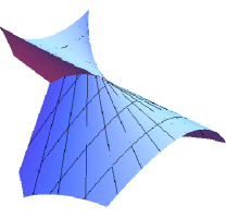
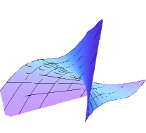
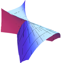
Figure 1: $f$ of $k=4,5,6$

Remark 3.4.

By the above construction, we can obtain the normal forms for singular points of $k$-th kind by the same mannar. For functions $g,h$,

$$\begin{array}[]{l}\Bigg{(}u,\displaystyle\left(\dfrac{v^{k}}{k!}-u\right)g^{(k)}+\sum_{i=1}^{k}(-1)^{i}\dfrac{v^{k-i}}{(k-i)!}g^{(k-i)}(u,v),\\ \hskip 85.35826pt\displaystyle\left(\dfrac{v^{k}}{k!}-u\right)h^{(k)}+\sum_{i=1}^{k}(-1)^{i}\dfrac{v^{k-i}}{(k-i)!}h^{(k-i)}(u,v)\Bigg{)}\end{array}$$ (3.7)

at $0$ is a $k$-th kind of singular point if $(g^{(k)},h^{(k)})(0,0)\neq(0,0).$ Moreover, if

$$\det{\begin{pmatrix}g^{(k+1)}(0)&g^{(k+2)}(0)\\ h^{(k+1)}(0)&g^{(k+2)}(0)\end{pmatrix}}\neq 0,$$

then it is a front. Here, $g^{\prime}=\partial g/\partial v=g^{(1)}$, and $g^{(i)}=\partial g^{(i-1)}/\partial v$, for example.

Example 3.5.

Let us set $g=v^{4}/4!$ and $h=u^{2}/2+v^{5}/5!$. Then the surface obtained by (3.7) is $(u,v)\mapsto(u,-uv+v^{4}/24,(-15u^{2}+15uv^{2}-v^{5})/30)$, and it can be drawn in Figure 2. This singularity is called cuspidal butterfly.

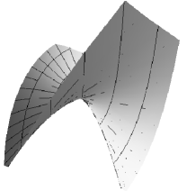
Figure 2: The surface of example 3.5.

3.2 Normal form that the singular set is the $u$-axis

The singular set $S(f)$ of $f$ in the form (3.6) is a parabola and the null vector field on $S(f)$ is constantly $\partial_{v}$. On the other hand, sometimes we want to have a form satisfying that the singular set is the $u$-axis, although the null vector field is not constant. For that purpose, take $f$ as in (3.6), and set $\tilde{f}(\tilde{u},\tilde{v})=f(\tilde{u}+\tilde{v}^{2}/2,\tilde{v})$. Then $F(x,y)=-\tilde{f}(-y,x)$ is a frontal, and $0$ is a singular point of the second kind satisfying $\eta=\partial_{u}+u\partial_{v}$ and $S(f)=\{v=0\}$.

3.3 Forms in the low degrees

In the Proposition 3.1, we have the normal forms in the low degrees in the following manner. In the form (3.6), we set

$$g(u,v)=g_{5}(u,v)+g_{6}(u,v),\quad h(u,v)=h_{5}(u,v)+h_{6}(u,v),$$

where $g_{6},h_{6}$ satisfy $j^{5}g_{6}(0,0)=j^{5}h_{6}(0,0)=0$, and $g_{5},h_{5}$ are

$$g_{5}(u,v)=\sum_{i+j=1}^{5}\dfrac{a_{ij}}{i!j!}u^{i}v^{j},\quad h_{5}(u,v)=\sum_{i+j=1}^{5}\dfrac{b_{ij}}{i!j!}u^{i}v^{j},$$

where $a_{ij},b_{ij}\in\boldsymbol{R}$ and $a_{02}=a_{10}$, $b_{02}=b_{10}$, $a_{03}\neq 0$, $b_{03}=0$. Then $f$ has the form

$$\begin{array}[]{l}\displaystyle\Bigg{(}u,\ \dfrac{-2a_{12}+a_{20}}{2}u^{2}+\dfrac{-3a_{22}+a_{30}}{6}u^{3}+\dfrac{-4a_{32}+a_{40}}{24}u^{4}-a_{03}uv-a_{13}u^{2}v-\dfrac{a_{23}}{2}u^{3}v\\[11.38109pt] \displaystyle\hskip 42.67912pt-\dfrac{a_{04}}{2}uv^{2}-\dfrac{a_{14}}{2}u^{2}v^{2}+\dfrac{a_{03}}{6}v^{3}+\dfrac{-a_{05}+a_{13}}{6}uv^{3}+\dfrac{a_{04}}{8}v^{4}+G(u,v),\\[11.38109pt] \displaystyle\hskip 85.35826pt\dfrac{-2b_{12}+b_{20}}{2}u^{2}+\dfrac{-3b_{22}+b_{30}}{6}u^{3}+\dfrac{-4b_{32}+b_{40}}{24}u^{4}-b_{13}u^{2}v-\dfrac{b_{23}}{2}u^{3}v\\[11.38109pt] \displaystyle\hskip 85.35826pt-\dfrac{b_{04}}{2}uv^{2}-\dfrac{b_{14}}{2}u^{2}v^{2}+\dfrac{-b_{05}+b_{13}}{6}uv^{3}+\dfrac{b_{04}}{8}v^{4}+H(u,v)\Bigg{)},\end{array}$$ (3.8)

where, $G,H$ are functions their $4$-jet vanishes: $j^{4}G(0,0)=j^{4}H(0,0)=0$, and

$$\begin{array}[]{l}G(u,v)=\dfrac{1}{2}(g_{5})_{vv}(u,v)v^{2}+\left(\dfrac{v^{2}}{2}-u\right)(g_{6})_{vv}(u,v)-v(g_{6})_{v}(u,v)+g_{6}(u,v)\\[11.38109pt] H(u,v)=\dfrac{1}{2}(h_{5})_{vv}(u,v)v^{2}+\left(\dfrac{v^{2}}{2}-u\right)(h_{6})_{vv}(u,v)-v(h_{6})_{v}(u,v)+h_{6}(u,v).\end{array}$$

3.4 Invariants

In [21], several invariants of singular points of the second kind are introduced. We take a parametrization $\gamma(t)$ of $S(f)$ and assume $\gamma(0)=0$. We set $\hat{\gamma}=f\circ\gamma$ as above. The limiting normal curvature $\kappa_{\nu}$ of $f$ at $0$ is defined by

$$\kappa_{\nu}(0)=\lim_{t\to 0}\dfrac{\left\langle{\hat{\gamma}^{\prime\prime}(t)},{\nu(\gamma(t))}\right\rangle}{|\hat{\gamma}(t)|^{2}}$$

with respect to the unit normal vector $\nu$ (cf. [21, (2.2)]), where $\hat{\gamma}$ is the singular locus. The normalized cuspidal curvature $\mu_{c}$ is defined by

$$\mu_{c}=\left.\dfrac{-|f_{u}|^{3}\left\langle{f_{uv}},{\nu_{v}}\right\rangle}{|f_{uv}\times f_{u}|^{2}}\right|_{(u,v)=(0,0)}$$

(cf. [21, (4.6)]), where $(u,v)$ is a coordinate system satisfying $\ker df_{0}=\left\langle{\partial v}\right\rangle_{\boldsymbol{R}}$. The limiting normal curvature and normalized cuspidal curvature relate the boundedness of the Gaussian and mean curvature near singular points of the second kind [21, Propositions 4.2, 4.3, Theorem 4.4]. The limiting singular curvature $\tau_{s}$ is defined by the limit of singular curvature [25] and it is computed by

$$\tau_{s}=\left.\dfrac{\det(\hat{\gamma}^{\prime\prime},\hat{\gamma}^{\prime\prime\prime},\nu(\gamma))}{|\hat{\gamma}^{\prime\prime}|^{5/2}}\right|_{t=0}$$

(cf. [21, p. 272, Proposition 4.9]). The limiting singular curvature measures the wideness of the cusp of the singular points of the second kind.

We assume that $f$ is a singular points of the second kind given in the form (3.8). Then

$$\kappa_{\nu}(u)=-2b_{12}+b_{20},\quad\mu_{c}=\dfrac{b_{04}}{{a_{03}}^{2}},\quad\tau_{s}=2a_{03},$$ (3.9)

where $\nu$ is the unit normal vector satisfying $\nu(0,0)=(0,0,1)$.

4 Geometric foliations near swallowtail

In this section, as an application of the normal form of swallowtail, we study geometric foliations near swallowtail defined by binary differential equations.

4.1 Binary differential equations

Let $U\subset\boldsymbol{R}^{2}$ be an open set and $(u,v)$ a coordinate system on $U$. Consider a $2$-tensor

$$\omega=p\,du^{2}+2q\,dudv+r\,dv^{2}$$ (4.1)

where $p,q,r$ are functions on $U$. If a vector field $X=x_{1}\partial_{u}+x_{2}\partial_{v}$ satisfies

$$\omega(X,X)=px_{1}^{2}+2qx_{1}x_{2}+rx_{2}^{2}=0,$$

then direction of $X$ is called the direction of $\omega=0$, and the integral curves of $X$ is called the solutions of $\omega=0$. We call $\omega=0$ a binary differential equation (BDE). We set $\delta=q^{2}-pr$. Then $\omega=0$ defines two linearly independent directions on $\{\delta>0\}\subset U$, and it defines one direction on $\{\delta=0\}$, and it defines no direction on $\{\delta<0\}$.

Definition 4.1.

Two BDEs $\omega_{1}=0$, $\omega_{2}=0$ are equivalent if there exist diffeomorphism $\Phi:(\boldsymbol{R}^{2},0)\to(\boldsymbol{R}^{2},0)$, and a function $\rho:(\boldsymbol{R}^{2},0)\to\boldsymbol{R}$ $(\rho(0)\neq 0)$ such that

$$\rho\ \Phi^{*}\omega_{1}=\omega_{2}.$$

We identify two BDEs if they are equivalent. If a $2$-tensor $\omega$ as in (4.1) satisfies $\delta(0)>0$, then the BDE $\omega=0$ is equivalent to $dx^{2}-dy^{2}=0$. We consider here the case $r(0)\neq 0$, $p_{u}(0)=0$, $p_{v}(0)\neq 0$ following [4], since only this case is needed for our consideration. See [3, 4, 7, 8] for general study of BDEs. Dividing $\omega$ by $r$, and putting $\tilde{p}=p/r$, $\tilde{q}=q/r$, we consider

$$\begin{array}[]{rl}\tilde{\omega}&=\tilde{p}\,du^{2}+2\tilde{q}\,dudv+dv^{2},\\ \tilde{p}&=p_{01}v+\dfrac{p_{20}}{2}u^{2}+p_{11}uv+\dfrac{p_{02}}{2}v^{2}+O(3),\quad p_{01}\neq 0\\ \tilde{q}&=q_{10}u+q_{01}v+\dfrac{q_{20}}{2}u^{2}+q_{11}uv+\dfrac{q_{02}}{2}v^{2}+O(3),\\ \end{array}$$ (4.2)

where $O(r)$ stands for the terms whose degrees are greater than or equal to $r$. We may assume $p_{01}>0$ without loss of generality. Considering the coordinate change

$$u=-\sqrt{p_{01}}\,U,\quad v=V-\dfrac{q_{10}}{2p_{01}}U^{2}+\dfrac{q_{01}}{\sqrt{p_{01}}}UV,$$

and dividing by the coefficient of $dv^{2}$, we see $\tilde{\omega}=0$ is equivalent to $(A/C)\,dU^{2}+2(B/C)\,dUdV+dV^{2}=0$, where

$$A =V+\dfrac{p_{20}-2q_{10}^{2}-p_{01}q_{10}}{2p_{01}^{2}}U^{2}-\dfrac{p_{11}-2q_{10}q_{01}-p_{01}q_{01}}{p_{01}\sqrt{p_{01}}}UV+\dfrac{p_{02}-2q_{01}^{2}}{2p_{01}}V^{2}+O(3)$$

$$2B =\dfrac{q_{10}q_{01}-q_{20}}{p_{01}\sqrt{p_{01}}}U^{2}-2\dfrac{q_{01}^{2}-q_{11}}{p_{01}}UV-\dfrac{q_{02}}{\sqrt{p_{01}}}V^{2}+O(3)$$

$$C =1+\dfrac{2q_{01}U}{\sqrt{p_{01}}}+\dfrac{q_{01}^{2}U^{2}}{p_{01}}+O(3)$$

and it is equal to $A^{\prime}\,dU^{2}+2B^{\prime}\,dUdV+dV^{2}=0$, where

$$A^{\prime} =V+\dfrac{p_{20}-2q_{10}^{2}-q_{10}p_{01}}{p_{01}^{2}}\dfrac{U^{2}}{2}-\dfrac{p_{11}-2q_{01}q_{10}+q_{01}p_{01}}{p_{01}\sqrt{p_{01}}}UV+\dfrac{p_{02}-2q_{01}^{2}}{p_{01}}\dfrac{V^{2}}{2}+O(3)$$

$$2B^{\prime} =\dfrac{q_{01}q_{10}-q_{20}}{p_{01}\sqrt{p_{01}}}U^{2}-2\dfrac{q_{01}^{2}-q_{11}}{p_{01}}UV-\dfrac{q_{02}}{\sqrt{p_{01}}}V^{2}+O(3)$$

Now we consider a BDE $\overline{\omega}=\overline{p}\,du^{2}+2\overline{q}\,dudv+dv^{2}=0$, where

$$\overline{p}=v+\dfrac{\overline{p}_{20}}{2}u^{2}+\overline{p}_{11}uv+\dfrac{\overline{p}_{02}}{2}v^{2}+O(3),\quad\overline{q}=\dfrac{\overline{q}_{20}}{2}u^{2}+\overline{q}_{11}uv+\dfrac{\overline{q}_{02}}{2}v^{2}+O(3),\quad p_{20}\neq 0.$$

Consider a coordinate transformation

$$u=U+\dfrac{x_{20}}{2}U^{2}+x_{11}UV,\quad v=V+\dfrac{x_{30}}{6}U^{3}+\dfrac{x_{21}}{2}U^{2}V+\dfrac{x_{12}}{2}UV^{2},$$

where

$$x_{20}=-\dfrac{\overline{p}_{11}}{2},\ x_{11}=-\dfrac{\overline{p}_{02}}{4},\ y_{30}=-\overline{q}_{20},\ y_{21}=\dfrac{-4\overline{q}_{11}+\overline{p}_{02}}{4},\ y_{12}=-\overline{p}_{02},$$

and dividing by the coefficient of $dv^{2}$, we see $\overline{\omega}=0$ is equivalent to $(P/R)\,dU^{2}+2(O(3)/R)\,dUdV+dV^{2}=0$, where

$$P=V+\dfrac{\overline{p}_{20}}{2}U^{2}+O(3),\quad R=1+(\overline{p}_{02}-4\overline{q}_{11})U^{2}/4-2\overline{q}_{02}UV+O(3)$$

and it is equal to $k=3$ of

$$\Big{(}V+\dfrac{\overline{p}_{20}}{2}U^{2}+O(k)\Big{)}\,dU^{2}+2O(k)\,dUdV+dV^{2}=0.$$ (4.3)

It known that for any $r\geq 3$, the BDE (4.3) is equivalent to $k=r$ of (4.3) ([4, Proposition 4.9] see also [7]). We set

$$A(\tilde{\omega})=\dfrac{p_{20}-2q_{10}^{2}-p_{01}q_{10}}{p_{01}^{2}}$$

for a BDE $\tilde{\omega}=0$ of the form (4.2). Summarizing up the above arguments, we have the following fact.

Fact 4.2.

For any $r\geq 3$, the BDE $\tilde{\omega}$ of the form (4.2) is equivalent to

$$\left(u+A(\tilde{\omega})\dfrac{u^{2}}{2}+O(r)\right)\,du^{2}+2O(r)\,dudv+dv^{2}=0.$$

On the other hand, the configuration of the solutions of the BDE

$$\omega_{l}=(v+lu^{2}/2)\,du^{2}+dv^{2}=0$$

is called folded saddle if $l<0$, called folded node if $0<l<1/8$, and called folded focus if $l>1/8$, and they are drawn as in Figure 3.

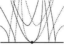
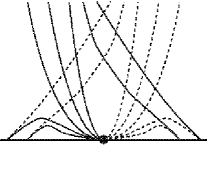
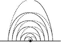
Figure 3: Configurations of $\omega_{k}$, folded saddle, folded node, folded focus.

4.2 Geometric foliations near swallowtail

Here we consider the following three $2$-tensors.

$$\begin{array}[]{rl}\omega_{lc}=&(FN-GM)\,du^{2}+(EN-GL)\,dudv+(EN-FL)\,dv^{2},\\ \omega_{as}=&L\,du^{2}+2M\,dudv+N\,dv^{2},\\ \omega_{ch}=&(L(GL-EN)+2M(EM-FL))\,du^{2}\\ &\hskip 28.45274pt+2(M(GL+EN)-2FLN)\,dudv\\ &\hskip 56.9055pt+(N(EN-GL)+2M(GM-FN))\,dv^{2}.\end{array}$$ (4.4)

The configuration of the solutions of $\omega_{lc}$ is called the lines of curvature, and that of $\omega_{as}$ is called the asymptotic curves. Since $\omega_{ch}=0$ can be deformed to

$$\begin{array}[]{cl}&(NH-GK)\,dv^{2}+2(MH-FK)\,dudv+(LH-EK)\,du^{2}=0\\[5.69054pt] \Leftrightarrow&\dfrac{N\,dv^{2}+2M\,dudv+L\,du^{2}}{G\,dv^{2}+2F\,dudv+E\,du^{2}}=\dfrac{K}{H}\left(=\dfrac{2}{\kappa_{1}^{-1}+\kappa_{2}^{-1}}\right),\end{array}$$

along the solution curves of $\omega_{ch}$, its normal curvature is equal to the harmonic mean of principal curvatures, where $K,H$ are the Gaussian and mean curvatures respectively. The discriminant of $\omega_{ch}=0$ is a positive multiplication of $K$. Thus the solutions of $\omega_{ch}=0$ lie in the region of positive Gaussian curvature. The the solutions of $\omega_{ch}=0$ is called characteristic curves (see [9, 13]). We consider three foliations of (4.4) near swallowtail. Configurations of these foliations near singular points are intensively studied. See [6, 7, 12, 13, 26, 27], for example. Let $\nu_{2}$ be a normal vector to $f$ where we do not assume $|\nu_{2}|=1$, and set $L_{2}=\left\langle{f_{uu}},{\nu_{2}}\right\rangle$, $M_{2}=\left\langle{f_{uv}},{\nu_{2}}\right\rangle$, $N_{2}=\left\langle{f_{vv}},{\nu_{2}}\right\rangle$. One can easily see that all BDEs of (4.4) are equivalent to that of changing $L,M,N$ to $L_{2},M_{2},N_{2}$.

We take the coordinate system as in subsection 3.2. Then the singular set is $\{v=0\}$ and the null vector field on the $u$-axis is $\partial_{u}+u\partial_{v}$. Thus $F_{v}(u,0)=0$ for any $u$. Hence there exists a vector valued function $\varphi$ such that $F_{u}(u,v)+uF_{v}(u,v)=v\varphi(u,v)$. We set

$$\tilde{E}_{2}=\left\langle{\varphi},{\varphi}\right\rangle,\ \tilde{F}_{2}=\left\langle{\varphi},{f_{v}}\right\rangle,\ \tilde{G}_{2}=\left\langle{f_{v}},{f_{v}}\right\rangle,$$

and

$$\tilde{L}_{2}=-\left\langle{\varphi},{(\nu_{2})_{u}}\right\rangle,\ \tilde{M}_{2}=-\left\langle{\varphi},{(\nu_{2})_{v}}\right\rangle,\ \tilde{N}_{2}=-\left\langle{f_{v}},{(\nu_{2})_{v}}\right\rangle.$$

Then

$$\omega_{lc}= v\Bigg{(}\Big{(}\tilde{F}\tilde{N}_{2}-\tilde{G}\tilde{M}_{2}\Big{)}\,du^{2}+\Big{(}-\tilde{G}\tilde{L}_{2}+\big{(}\tilde{G}\tilde{M}_{2}-2\tilde{F}\tilde{N}_{2}\big{)}u+\tilde{E}\tilde{N}_{2}v\Big{)}\,dudv$$

$$\hskip 14.22636pt+\Big{(}\tilde{G}\tilde{L}_{2}u-\tilde{F}\tilde{L}_{2}v+\tilde{F}\tilde{N}_{2}u^{2}+\big{(}-\tilde{F}\tilde{M}_{2}-\tilde{E}\tilde{N}_{2}\big{)}uv+\tilde{E}\tilde{M}_{2}v^{2}\Big{)}\,dv^{2}\Bigg{)},$$ (4.5)

$$\omega_{as}= \Big{(}\tilde{L}_{2}v+\tilde{N}_{2}u^{2}-\tilde{M}_{2}uv\Big{)}\,du^{2}+2\Big{(}-\tilde{N}_{2}u+\tilde{M}_{2}v\Big{)}\,dudv+\tilde{N}_{2}\,dv^{2},$$ (4.6)

$$\omega_{ch}= v\Bigg{(}\Big{(}\tilde{G}\tilde{L}_{2}^{2}v-\tilde{G}\tilde{L}_{2}\tilde{N}_{2}u^{2}+4\tilde{F}\tilde{L}_{2}\tilde{N}_{2}uv-\big{(}2\tilde{F}\tilde{L}_{2}\tilde{M}_{2}+\tilde{E}\tilde{L}_{2}\tilde{N}_{2}\big{)}v^{2}$$

$$\hskip 42.67912pt-\tilde{G}\tilde{M}_{2}\tilde{N}_{2}u^{3}+\big{(}\tilde{G}\tilde{M}_{2}^{2}+2\tilde{F}\tilde{M}_{2}\tilde{N}_{2}+\tilde{E}\tilde{N}_{2}^{2}\big{)}u^{2}v$$

$$\hskip 71.13188pt-\big{(}2\tilde{F}\tilde{M}_{2}^{2}+3\tilde{E}\tilde{M}_{2}\tilde{N}_{2}\big{)}uv^{2}+2\tilde{E}\tilde{M}_{2}^{2}v^{3}\Big{)}\,du^{2}$$

$$\hskip 14.22636pt+2\Big{(}\tilde{G}\tilde{L}_{2}\tilde{N}_{2}u+\big{(}\tilde{G}\tilde{L}_{2}\tilde{M}_{2}-2\tilde{F}\tilde{L}_{2}\tilde{N}_{2}\big{)}v$$

$$\hskip 42.67912pt+\tilde{G}\tilde{M}_{2}\tilde{N}_{2}u^{2}-\big{(}\tilde{G}\tilde{M}_{2}^{2}+\tilde{E}\tilde{N}_{2}^{2}\big{)}uv+\tilde{E}\tilde{M}_{2}\tilde{N}_{2}v^{2}\Big{)}\,dudv$$

$$+\Big{(}-\tilde{G}\tilde{L}_{2}\tilde{N}_{2}-\tilde{G}\tilde{M}_{2}\tilde{N}_{2}u+\big{(}2\tilde{G}\tilde{M}_{2}^{2}-2\tilde{F}\tilde{M}_{2}\tilde{N}_{2}+\tilde{E}\tilde{N}_{2}^{2}\big{)}v\Big{)}\,dv^{2}\Bigg{)}.$$ (4.7)

We factor out it from $\omega_{lc}$ and $\omega_{ch}$ and set

$$\tilde{\omega}_{lc}=\omega_{lc}/v,\quad\tilde{\omega}_{as}=\omega_{as},\quad\tilde{\omega}_{ch}=\omega_{ch}/v.$$

We consider the solutions of $\tilde{\omega}_{lc}$, $\tilde{\omega}_{as}$ and $\tilde{\omega}_{ch}$ instead of $\omega_{lc}$, $\omega_{as}$ and $\omega_{ch}$. Let us consider $\tilde{\omega}_{lc}=0$. Then the discriminant $\delta$ of $\tilde{\omega}_{lc}=0$ satisfies $\delta(0)>0$. It is known that such BDE is equivalent to $dx^{2}-dy^{2}=0$, and its configuration is a pair of transverse smooth foliations. Existence of lines of curvature coordinate system near swallowtail is shown by [22]. Let us consider $\tilde{\omega}_{as}=0$ and $\tilde{\omega}_{ch}=0$. We set $\tilde{\omega}_{as}=p_{as}\,du^{2}+2q_{as}\,dudv+r_{as}\,dv^{2}$ and $\tilde{\omega}_{ch}=p_{ch}\,du^{2}+2q_{ch}\,dudv+r_{ch}\,dv^{2}$. We assume that $\kappa_{\nu}(0)=-2b_{12}+b_{20}\neq 0$. Then $r_{as}$ and $r_{ch}$ does not vanish at $0$. Thus $\tilde{\omega}_{as}$ (respectively, $\tilde{\omega}_{ch}$) is equivalent to

$$\bar{\omega}_{as}=\dfrac{p_{as}}{r_{as}}\,du^{2}+2\dfrac{q_{as}}{r_{as}}\,dudv+dv^{2}\quad\Big{(}\text{respectively, }\bar{\omega}_{ch}=\dfrac{p_{ch}}{r_{ch}}\,du^{2}+2\dfrac{q_{ch}}{r_{ch}}\,dudv+dv^{2}\Big{)}.$$

We see that

$$\dfrac{p_{as}}{r_{as}}=-\dfrac{b_{04}}{2b_{12}-b_{20}}v+u^{2}+*uv+*v^{2}+O(3),\quad\dfrac{q_{as}}{r_{as}}=-u+*v+O(2)$$

and

$$\dfrac{p_{as}}{r_{as}}=\dfrac{b_{04}}{2b_{12}-b_{20}}v+u^{2}+*uv+*v^{2}+O(3),\quad\dfrac{q_{as}}{r_{as}}=-u+*v+O(2).$$

By (3.9), we have

$$A(\tilde{\omega}_{as})=-\dfrac{b_{04}}{2b_{12}-b_{20}}=-\dfrac{\mu_{c}\tau_{s}}{4\kappa_{\nu}}\quad\left(\text{respectively, }A(\tilde{\omega}_{ch})=\dfrac{b_{04}}{2b_{12}-b_{20}}=\dfrac{\mu_{c}\tau_{s}}{4\kappa_{\nu}}\right).$$

Thus we know the configuration of the solutions of $\tilde{\omega}_{as}$ is folded saddle if $l=-\mu_{c}\tau_{s}/(4\kappa_{\nu})$ $<0$, folded node if $0<l<1/8$, and folded focus if $1/8<l$. The same holds for $\tilde{\omega}_{ch}$ by setting $l=-\mu_{c}\tau_{s}/(4\kappa_{\nu})<0$.

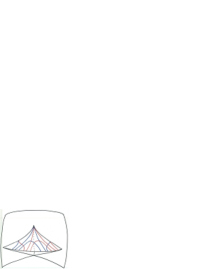
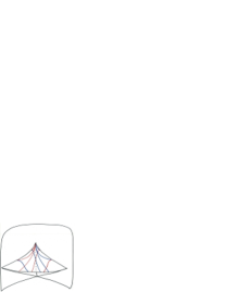
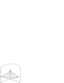
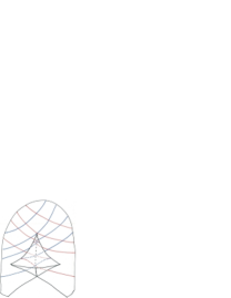
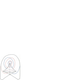
Figure 4: Geometric foliations on swallowtail

We can draw models of $\tilde{\omega}_{as}$ and $\tilde{\omega}_{ch}$ at swallowtails as in Figure 4. Since swallowtails appear as points on fronts, we would like to say that the generic configuration of $\tilde{\omega}_{as}$ and $\tilde{\omega}_{ch}$ are the these types. We note that since $\tilde{\omega}_{as}|_{v=0}=\tilde{N}_{2}(u^{2}\,du^{2}-2u\,dudv+dv^{2})$, $\tilde{\omega}_{ch}|_{v=0}=-(\tilde{N}\tilde{L}_{2}\tilde{N}_{2}(u^{2}\,du^{2}-2u\,dudv+dv^{2})$, the direction of $\tilde{\omega}_{as}$ and $\tilde{\omega}_{ch}$ are not the direction of the null vector field, the solutions of them on $S(f)$ forms $3/2$-cusps on the image of $f$.

Department of Mathematics,

Kobe University, Rokko 1-1, Nada,

Kobe 657-8501, Japan

sajiO​​​amath.kobe-u.ac.jp

References

- [1] V. I. Arnold, S. M. Gusein-Zade and A. N. Varchenko, Singularities of differentiable maps, Vol. 1, Monographs in Mathematics 82, Birkhäuser, Boston, 1985.
- [2] J. W. Bruce and F. Tari, Implicit differential equations from the singularity theory viewpoint, Singularities and differential equations (Warsaw, 1993), 23–38, Banach Center Publ., 33, Polish Acad. Sci. Inst. Math., Warsaw, 1996.
- [3] J. W. Bruce and F. Tari, On binary differential equations, Nonlinearity 8 (1995), no. 2, 255–271.
- [4] J. W. Bruce and F. Tari, Implicit differential equations from the singularity theory viewpoint, Singularities and differential equations (Warsaw, 1993), 23–38, Banach Center Publ., 33, Polish Acad. Sci. Inst. Math., Warsaw, 1996.
- [5] J. W. Bruce and J. West, Bruce, J. W.; West, J. M. Functions on a crosscap, Math. Proc. Cambridge Philos. Soc. 123 (1998), no. 1, 19–39.
- [6] L. Dara, Singularités génériques des équations differentielles multiformes, Bol. Soc. Brasil Math. 6 (1975), 95–128.
- [7] A. A. Davydov, Normal forms of differential equations unresolved with respect to derivatives in a neighbourhood of its singular point, Functional Anal. Appl. 19 (1985), 1–10.
- [8] A. A. Davydov, Qualitative Theory of Control Systems, Translations of Mathematical Monographs 142, American Mathematical Society, Providence, R.I. Moscow 1994.
- [9] L. P. Eisenhart, A treatise on the differential geometry of curves and surfaces, Dover Publications, Inc., New York 1960.
- [10] S. Fujimori, K. Saji, M. Umehara and K. Yamada, Singularities of maximal surfaces, Math. Z. 259 (2008), 827–848.
- [11] T. Fukui, Local differential geometry of cuspidal edge and swallowtail, preprint.
- [12] R. Garcia, C. Gutierrez and J. Sotomayor, Lines of principal curvature around umbilics and Whitney umbrellas, Tohoku Math. J., 52 (2000), 163–172.
- [13] R. Garcia and J. Sotomayor, Harmonic mean curvature lines on surfaces immersed in , Bull. Braz. Math. Soc. (N.S.) 34 (2003), no. 2, 303–331.
- [14] M. Hasegawa, A. Honda, K. Naokawa, K. Saji, M. Umehara and K. Yamada, Intrinsic properties of singularities of surfaces, Internat. J. Math. 26, 4 (2015) 1540008 (34 pages).
- [15] M. Hasegawa, A. Honda, K. Naokawa, M. Umehara and K. Yamada, Intrinsic Invariants of Cross Caps, Selecta Math. 20, 3, (2014) 769–785.
- [16] A. Honda, K. Naokawa, M. Umehara and K. Yamada, Isometric realization of cross caps as formal power series and its applications, preprint, arXiv:1601.06265.
- [17] S. Izumiya and S. Otani, Flat Approximations of surfaces along curves, Demonstr. Math. 48 (2015), no. 2, 217–241.
- [18] S. Izumiya, K. Saji and N. Takeichi, Flat surfaces along cuspidal edges, preprint.
- [19] M. Kokubu, W. Rossman, K. Saji, M. Umehara and K. Yamada, Singularities of flat fronts in hyperbolic -space, Pacific J. Math. 221 (2005), 303–351.
- [20] L. F. Martins and K. Saji, Geometric invariants of cuspidal edges, Canad. J. Math. 68 (2016), 445–462.
- [21] L. F. Martins, K. Saji, M. Umehara and K. Yamada, Behavior of Gaussian curvature near non-degenerate singular points on wave fronts, Geometry and topology of manifolds, 247–281, Springer Proc. Math. Stat., 154, Springer, Tokyo, 2016,
- [22] S. Murata and M. Umehara, Flat surfaces with singularities in Euclidean -space, J. Differential Geom. 82 (2009), 279–316.
- [23] K. Naokawa, M. Umehara and K. Yamada, Isometric deformations of cuspidal edges, Tohoku Math. J. (2) 68, 1 (2016), 73–90.
- [24] R. Oset Sinha and F. Tari, On the flat geometry of the cuspidal edge, preprint, arXiv:1610.08702.
- [25] K. Saji, M. Umehara and K. Yamada, The geometry of fronts, Ann. of Math. 169 (2009), 491–529.
- [26] F. Tari, On pairs of geometric foliations on a cross-cap, Tohoku Math. J. (2) 59 (2007), no. 2, 233–258.
- [27] F. Tari, Pairs of foliations on surfaces, Real and complex singularities, 305–337, London Math. Soc. Lecture Note Ser., 380, Cambridge Univ. Press, Cambridge, 2010.
- [28] J. West, The differential geometry of the cross-cap, PhD. thesis, University of Liverpool (1995)