On pairs of geometric foliations on a cuspidal edge

Kentaro Saji

We study the topological configurations of the lines of principal curvature, the asymptotic and characteristic curves on a cuspidal edge, in the domain of a parametrization of this surface as well as on the surface itself. Such configurations are determined by the $3$-jets of a parametrization of the surface.

000Partly supported by the Japan Society for the Promotion of Science (JSPS) and the Coordenadoria de AperfeiΓ§oamento de Pessoal de NΓ­vel Superior under the Japan-Brazil research cooperative program and the Grant-in-Aid for Scientific Research (Young Scientists (B)) No. 26400087, from JSPS.000 2010 Mathematics Subject classification. Primary 53A05; Secondary 58K05, 57R45.000Keywords and Phrases. Cuspidal edge, principal configuration, lines of curvature

1 Introduction and preliminaries about cuspidal edges

A singular point $x$ of a map $f:(\boldsymbol{R}^{2},x)\to(\boldsymbol{R}^{3},0)$ is called a cuspidal edge if the map-germ $f$ at $x$ is $\mathcal{A}$-equivalent to $(u,v)\mapsto(u,v^{2},v^{3})$ at 00. (Two map-germs $f_{1},f_{2}:(\boldsymbol{R}^{n},0)\to(\boldsymbol{R}^{m},0)$ are $\mathcal{A}$-equivalent if there exist diffeomorphisms $S:(\boldsymbol{R}^{n},0)\to(\boldsymbol{R}^{n},0)$ and $T:(\boldsymbol{R}^{m},0)\to(\boldsymbol{R}^{m},0)$ such that $f_{2}\circ S=T\circ f_{1}$.) If the singular point $x$ of $f$ is a cuspidal edge, then $f$ at $x$ is a front in the sense of [1] (see also [21]), and furthermore, they are one of two types of generic singularities of fronts (the other one is a swallowtail which is a singular point $u$ of $f$ satisfying that $f$ at $u$ is $\mathcal{A}$-equivalent to $(u,v)\mapsto(u,u^{2}v+3u^{4},2uv+4u^{3})$ at 00).

It is shown in [22] that a cuspidal edge can locally be parametrized after smooth changes of coordinates in the source and isometries in the target by

$$f(u,v)=\left(u,a_{1}(u)+\dfrac{v^{2}}{2},b_{2}(u)+v^{2}b_{3}(u)+v^{3}b_{4}(u,v)\right),$$ (1.1)

where $a_{1}(u),b_{2}(u),b_{3}(u),b_{4}(u,v)$ are $C^{\infty}$-functions satisfying $a_{1}(0)=a_{1}^{\prime}(0)=b_{2}(0)=b_{2}^{\prime}(0)=b_{3}(0)=0$, $b_{2}^{\prime\prime}(0)>0$, b4​(0,0)β‰ 0subscript𝑏4000b_{4}(0,0)\neq 0. Writing $a_{1}(u)=a_{20}u^{2}/2+a_{30}u^{3}/6+u^{4}h_{1}(u)$, $b_{2}(u)=b_{20}u^{2}/2+b_{30}u^{3}/6+u^{4}h_{2}(u)$, $b_{3}(u)=b_{12}u/2+u^{2}h_{3}(u)$, $b_{4}(u,v)=b_{03}/6+uh_{4}(u)+vh_{5}(u,v)$, we have

$$\begin{array}[]{L}f(u,v)=\displaystyle\Big{(}u,\frac{a_{20}}{2}u^{2}+\frac{a_{30}}{6}u^{3}+\frac{v^{2}}{2},\\ \hskip 56.9055pt\frac{b_{20}}{2}u^{2}+\frac{b_{30}}{6}u^{3}+\frac{b_{12}}{2}uv^{2}+\frac{b_{03}}{6}v^{3}\Big{)}+h(u,v),\end{array}$$ (1.2)

where b03β‰ 0,b20β‰₯0formulae-sequencesubscript𝑏030subscript𝑏200b_{03}\neq 0,\ b_{20}\geq 0 and

$$h(u,v)=\big{(}0,\,u^{4}h_{1}(u),u^{4}h_{2}(u)+u^{2}v^{2}h_{3}(u)+uv^{3}h_{4}(u)+v^{4}h_{5}(u,v)\big{)},$$

with $h_{1}(u),h_{2}(u),h_{3}(u),h_{4}(u),h_{5}(u,v)$ smooth functions. Several differential geometric invariants of cuspidal edges are investigated ([20, 22, 23, 25, 27, 28]), and coefficients of (1.2) are such invariants. According to [22], it is known that $a_{20}$ coincides with the singular curvature ΞΊssubscriptπœ…π‘ \kappa_{s}, $b_{20}$ coincides with the limiting normal curvature $\kappa_{\nu}$, $b_{03}$ coincides with the cuspidal curvature $\kappa_{c}$ and $b_{12}$ coincides with the cusp-directional torsion $\kappa_{t}$ at the origin. The singular curvature is the geodesic curvature of the singular set with sign, and the limiting normal curvature is the normal curvature of the singular set, and they relates to the shape of cuspidal edge (see [28]). The cuspidal curvature measures the wideness of the cusp, and the cusp-directional torsion measures the rotating ratio of the cusp along the singular set (see [22, 23]).

On the other hand, let $U\subset\boldsymbol{R}^{2}$ be an open subset and $(u,v)$ a coordinate system on $U$. Let

$$\omega=a(u,v)dv^{2}+2b(u,v)dudv+c(u,v)du^{2}$$ (1.3)

be a $2$-tensor on $U$, where $a,b,c$ are smooth functions, called the coefficients of $\omega$. We call $\omega=0$ a binary differential equation $($BDE$)$ corresponding to $\omega$. If $b^{2}-ac>0$ at $x\in U$, then $\omega(x)=0$ defines two directions in $T_{x}U$, and integral curves of these directions for two smooth and transverse foliations, called foliations with respect to $\omega$. If $b^{2}-ac=0$ at $x\in U$, then generically $\omega(x)=0$ defines a single direction, and the integral curves form in general a family of cusps. Thus we are mainly interested in behavior of integral curves of a BDE near a point where $b^{2}-ac$ vanishes. We call discriminant of a BDE the set where $b^{2}-ac=0$. If the single direction is transverse to the discriminant, then the BDE is equivalent to $dv^{2}+udu^{2}=0$ ([7, 8]). The normal form for the stable cases when the single direction is tangent to the discriminant is obtained in [9, 10]. Topological classifications of generic families of BDEs are obtained in [3, 5, 6, 26, 29, 32]. On the other hand, BDEs as geometric foliations on surfaces in three space is studied in [2, 12, 15, 16, 17, 29]. See [11, 18, 19] for other approaches for geometric foliations.

In this paper, following [12, 13, 15, 26, 29], we stick to special BDEs from differential geometry of surface in $\boldsymbol{R}^{3}$. There are three fundamental BDEs on a regular surface in $\boldsymbol{R}^{3}$. Let $f:(\boldsymbol{R}^{2},0)\to(\boldsymbol{R}^{3},0)$ be a regular surface with a unit normal vector field $\nu$. Let $\omega_{lc}$, Ο‰a​ssubscriptπœ”π‘Žπ‘ \omega_{as} and $\omega_{ch}$ be $2$-tensors defined by

Ο‰l​c=(E​Mβˆ’F​L)​d​v2+(E​Nβˆ’G​L)​d​u​d​v+(F​Nβˆ’G​M)​d​u2,Ο‰a​s=N​d​v2+2​M​d​u​d​v+L​d​u2,Ο‰c​h=(2​M​(G​Mβˆ’F​N)βˆ’N​(G​Lβˆ’E​N))​d​v2+2​(M​(G​L+E​N)βˆ’2​F​L​N)​d​u​d​v+(L​(G​Lβˆ’E​N)βˆ’2​M​(F​Lβˆ’E​M))​d​u2,subscriptπœ”π‘™π‘πΈπ‘€πΉπΏπ‘‘superscript𝑣2𝐸𝑁𝐺𝐿𝑑𝑒𝑑𝑣𝐹𝑁𝐺𝑀𝑑superscript𝑒2subscriptπœ”π‘Žπ‘ π‘π‘‘superscript𝑣22𝑀𝑑𝑒𝑑𝑣𝐿𝑑superscript𝑒2subscriptπœ”π‘β„Ž2𝑀𝐺𝑀𝐹𝑁𝑁𝐺𝐿𝐸𝑁𝑑superscript𝑣2missing-subexpressionmissing-subexpression2𝑀𝐺𝐿𝐸𝑁2𝐹𝐿𝑁𝑑𝑒𝑑𝑣missing-subexpressionmissing-subexpression𝐿𝐺𝐿𝐸𝑁2𝑀𝐹𝐿𝐸𝑀𝑑superscript𝑒2\begin{array}[]{rcl}\omega_{lc}&=&(EM-FL)dv^{2}+(EN-GL)dudv+(FN-GM)du^{2},\\ \omega_{as}&=&N\,dv^{2}+2M\,dudv+L\,du^{2},\\ \omega_{ch}&=&\big{(}2M(GM-FN)-N(GL-EN)\big{)}\,dv^{2}\\ &&\hskip 28.45274pt+2\big{(}M(GL+EN)-2FLN\big{)}\,dudv\\ &&\hskip 56.9055pt+\big{(}L(GL-EN)-2M(FL-EM)\big{)}\,du^{2},\end{array}

where $(u,v)$ is a coordinate system on $(\boldsymbol{R}^{2},0)$, and

$${\begin{pmatrix}E&F\\ F&G\end{pmatrix}}={\begin{pmatrix}\left\langle{f_{u}},{f_{u}}\right\rangle&\left\langle{f_{u}},{f_{v}}\right\rangle\\ \left\langle{f_{v}},{f_{u}}\right\rangle&\left\langle{f_{v}},{f_{v}}\right\rangle\end{pmatrix}},\ {\begin{pmatrix}L&M\\ M&N\end{pmatrix}}={\begin{pmatrix}\left\langle{f_{uu}},{\nu}\right\rangle&\left\langle{f_{uv}},{\nu}\right\rangle\\ \left\langle{f_{uv}},{\nu}\right\rangle&\left\langle{f_{vv}},{\nu}\right\rangle\end{pmatrix}},$$

where $\left\langle{~{}},{~{}}\right\rangle$ stands for the standard inner product of $\boldsymbol{R}^{3}$. Each integral curve of the foliations with respect to $\omega_{lc}$ is called a line of curvature, each integral curve with respect to Ο‰a​ssubscriptπœ”π‘Žπ‘ \omega_{as} is called an asymptotic curve and each integral curve with respect to $\omega_{ch}$ is called a characteristic curve or harmonic mean curvature curve. Asymptotic curves appear only on a domain where the Gaussian curvature $K$ of $f$ is non-negative, and characteristic curves appear only on a domain where the Gaussian curvature $K$ of $f$ is non-positive. Since $\omega_{ch}=0$ can be deformed as

$$\begin{array}[]{cl}&(NH-GK)\,dv^{2}+2(MH-FK)\,dudv+(LH-EK)\,du^{2}=0\\[5.69054pt] \Leftrightarrow&\dfrac{N\,dv^{2}+2M\,dudv+L\,du^{2}}{G\,dv^{2}+2F\,dudv+E\,du^{2}}=\dfrac{K}{H}\left(=\dfrac{2}{\kappa_{1}^{-1}+\kappa_{2}^{-1}}\right),\end{array}$$

where $K$ is the Gaussian curvature, $H$ is the mean curvature, and $\kappa_{1}$, $\kappa_{2}$ are the principal curvatures of $f$, we see that along the characteristic curve, the normal curvature of it is equal to the harmonic mean of the principal curvatures (see [13], for example).

Acknowledgements.

This paper is prepared while the author was visiting Luciana Martins at IBILCE - UNESP. He would like to thank Luciana Martins for fruitful discussions. He would also like to thank Farid Tari for valuable comments. He would also like to thank the referee for careful reading and helpful suggestions.

2 Preliminaries on BDEs

In this section, following [5, 6], we introduce a method to study the configurations of the solution curves of a BDE. Let $\omega(u,v)$ be the $2$-tensor on $(U;(u,v))\subset\boldsymbol{R}^{2}$ as in (1.3). If (a,b,c)β‰ (0,0,0)π‘Žπ‘π‘000(a,b,c)\neq(0,0,0) at $x\in U$, then $\omega$ is called of Type $1$ at $x$, and if $(a,b,c)=(0,0,0)$ at $x\in U$, then $\omega$ is called of Type $2$ at $x$. If $\omega$ is of Type 2 at $x$, then $\delta=b^{2}-ac$ has a critical point at $x$. Since we are interested in local behavior of $\omega$, we set $x=(0,0)$. If $\omega$ is of Type 1, then $\omega$ defines a single direction at points on $\Delta$, and if it is of Type 2, then all directions in the plane are solutions of $\omega=0$ at that point. Moreover, if $\omega$ is of Type $2$ at $x$, then $\Delta$ is not a smooth curve. We are interested in the configurations of the foliations of $\omega=0$. We define the following equivalence.

Definition 2.1.

Two binary differential equations $\omega_{1}=0$ and $\omega_{2}=0$ are equivalent if there exist a diffeomorphism germ $\Phi:(\boldsymbol{R}^{2},0)\to(\boldsymbol{R}^{2},0)$ and a non-zero function $\rho:(\boldsymbol{R}^{2},0)\to\boldsymbol{R}$ such that $\rho\big{(}\Phi^{*}\omega_{1}\big{)}=\omega_{2}$ holds. If $\Phi$ is a homeomorphism such that $\Phi$ takes the integral curves of $\omega_{1}$ to those of $\omega_{2}$, they are called topologically equivalent.

If two binary differential equations are equivalent then the configurations of their foliations can be regarded the same. To obtain the topological configurations, we use the following method developed in [5, 6, 12, 15, 29, 30]. We separate our consideration into the following three cases:

  • β€’

    Case 1: (a​(0),b​(0),c​(0))β‰ (0,0,0)π‘Ž0𝑏0𝑐0000(a(0),b(0),c(0))\neq(0,0,0) and δ​(0)β‰ 0𝛿00\delta(0)\neq 0 (Type 1).

  • β€’

    Case 2: (a​(0),b​(0),c​(0))β‰ (0,0,0)π‘Ž0𝑏0𝑐0000(a(0),b(0),c(0))\neq(0,0,0) and $\delta(0)=0$ (Type 1).

  • β€’

    Case 3: $(a(0),b(0),c(0))=(0,0,0)$ (Type 2).

Consider the associated surface to $\omega$

$$\mathcal{M}=\{(u,v,[\alpha,\beta])\in(\boldsymbol{R}^{2},0)\times\boldsymbol{R}P^{1}\,|\,a\beta^{2}+2b\alpha\beta+c\alpha^{2}=0\}.$$

Then $\mathcal{M}$ is a smooth manifold if b2βˆ’a​cβ‰ 0superscript𝑏2π‘Žπ‘0b^{2}-ac\neq 0, or if $a_{u}+2b_{u}p+c_{u}p^{2}=0$ and $a_{v}+2b_{v}p+c_{v}p^{2}=0$ do not have any common root. The second condition is equivalent to

det(au2​bucu00au2​bucuav2​bvcv00av2​bvcv)​(0)β‰ 0.matrixsubscriptπ‘Žπ‘’2subscript𝑏𝑒subscript𝑐𝑒00subscriptπ‘Žπ‘’2subscript𝑏𝑒subscript𝑐𝑒subscriptπ‘Žπ‘£2subscript𝑏𝑣subscript𝑐𝑣00subscriptπ‘Žπ‘£2subscript𝑏𝑣subscript𝑐𝑣00\det{\begin{pmatrix}a_{u}&2b_{u}&c_{u}&0\\ 0&a_{u}&2b_{u}&c_{u}\\ a_{v}&2b_{v}&c_{v}&0\\ 0&a_{v}&2b_{v}&c_{v}\end{pmatrix}}(0)\neq 0. (2.1)

Consider the projection $\pi:\mathcal{M}\to\boldsymbol{R}^{2}$, $\pi(u,v,[\alpha:\beta])=(u,v)$. Then $\pi^{-1}(u,v)$ consists of two points if $b^{2}-ac>0$, and is empty if $b^{2}-ac<0$. Let us set $p=\beta/\alpha$ (we need to consider the case $q=\alpha/\beta$ for some cases) and $\mathcal{F}(u,v,p)=ap^{2}+2bp+c$. If β„±p​(0)β‰ 0subscriptℱ𝑝00\mathcal{F}_{p}(0)\neq 0, then $\pi$ is a local diffeomorphism, and if $\mathcal{F}_{p}(0)=0$ and β„±p​p​(0)β‰ 0subscriptℱ𝑝𝑝00\mathcal{F}_{pp}(0)\neq 0 hold, then $\pi$ is a fold (a map-germ $h:(\boldsymbol{R}^{2},0)\to(\boldsymbol{R}^{2},0)$ is a fold if $h$ is $\mathcal{A}$-equivalent to $(u,v)\mapsto(u,v^{2})$). Let us consider the vector field

$$\xi(u,v,p)=p\mathcal{F}_{p}(u,v,p)\partial_{u}+\mathcal{F}_{p}(u,v,p)\partial_{v}-\big{(}p\mathcal{F}_{u}(u,v,p)+\mathcal{F}_{v}(u,v,p)\big{)}\partial p.$$

Then $\xi$ is tangent to $\mathcal{M}$, and the projections $d\pi(\xi_{1}),d\pi(\xi_{2})$ satisfy

$$\omega(d\pi(\xi_{i}),d\pi(\xi_{i}))=0\quad(i=1,2),$$

where $\xi_{i}=\xi(u,v,p_{i})$ and $\pi^{-1}(u,v)$ $=$ $\{(u,v,p_{1}),(u,v,p_{2})\}$, or $\pi^{-1}(u,v)$ $=$ $\{(u,v,p_{1})\}$. To study geometric the foliations of $\omega$, we use $\xi$ on $\mathcal{M}$.

2.1 Case 1

We assume that $b^{2}-ac>0$ at 00. Then one can easily see that the BDE (1.3) is equivalent to a BDE $a\,dv^{2}+2b\,dudv+c\,du^{2}=0$ which satisfies $(a(0,0),b(0,0),c(0,0))=(1,0,-1)$. Furthermore, it holds that for any $k>0$, a BDE $a\,dv^{2}+2b\,dudv+c\,du^{2}=0$ which satisfies $(a(0,0),b(0,0),c(0,0))=(1,0,-1)$ is equivalent to a BDE $a\,dv^{2}+2b\,dudv+c\,du^{2}=0$ whose $k$-jet of $(a,b,c)$ at $(0,0)$ is $(1,0,-1)$, moreover, it is equivalent to a BDE

$$\omega_{reg}=dv^{2}-du^{2}=0$$ (2.2)

([6, Proposition 4.4]). Therefore the configuration is a pair of transverse smooth foliations.

2.2 Case 2

We consider the case 2, namely (a​(0),b​(0),c​(0))β‰ (0,0,0)π‘Ž0𝑏0𝑐0000(a(0),b(0),c(0))\neq(0,0,0) and $\delta(0)=0$.

Lemma 2.2.

We assume that (a​(0),b​(0),c​(0))β‰ (0,0,0)π‘Ž0𝑏0𝑐0000(a(0),b(0),c(0))\neq(0,0,0) and
$\delta(0)$ $=0$. If $\omega$ as in (1.3) satisfies

$$j^{1}(a,b,c)(0,0)=(0,0,\alpha_{0})+(\alpha_{1}v,\alpha_{2}v,\alpha_{3}u+\alpha_{4}v),$$

then it is equivalent to a BDE $a\,dv^{2}+2b\,dudv+c\,du^{2}=0$ which satisfies

$$(j^{1}a(0,0),j^{1}b(0,0),j^{1}c(0,0))=(1,0,u)$$

when Ξ±0​α1β‰ 0subscript𝛼0subscript𝛼10\alpha_{0}\alpha_{1}\neq 0.

Proof.

We assume that Ξ±0​α1β‰ 0subscript𝛼0subscript𝛼10\alpha_{0}\alpha_{1}\neq 0. Consider $u=V+\beta_{1}U^{2}+\beta_{2}V^{2},\ v=U$ and $R=1+\beta_{3}U$, where $\beta_{1},\beta_{2},\beta_{3}\in\boldsymbol{R}$. Then $R\omega(U,V)$ is given by

$$\begin{array}[]{l}\big{(}\alpha_{1}U+O(2)\big{)}\,dV^{2}+\big{(}2(\alpha_{2}+2\alpha_{0}\beta_{1})U+O(2)\big{)}\,dUdV\\ \hskip 56.9055pt+\big{(}\alpha_{0}+(\alpha_{4}+\alpha_{0}\beta_{3})U+(\alpha_{3}+4\alpha_{0}\beta_{2})V+O(2)\big{)}\,dU^{2},\end{array}$$

where $O(2)$ stands for remainders of order $2$. Setting $\beta_{1}=-\alpha_{2}/(2\alpha_{0})$, $\beta_{2}=-\alpha_{3}/(4\alpha_{0})$ and $\beta_{3}=-\alpha_{4}/\alpha_{0}$, and re-scaling, we get the desired result. ∎

Any BDE of the form (1.3) with $(j^{1}a(0,0),j^{1}b(0,0),j^{1}c(0,0))=(1,0,u)$ is smoothly equivalent to

Ο‰c​u​s​p=d​v2+u​d​u2=0subscriptπœ”π‘π‘’π‘ π‘π‘‘superscript𝑣2𝑒𝑑superscript𝑒20\omega_{cusp}=dv^{2}+u\,du^{2}=0 (2.3)

([8], see also [6, Section 4.2], [30, Proposition 3.3-2]). The solutions form a family of cusps.

2.3 Case 3

We assume $(a(0),b(0),c(0))=(0,0,0)$. In this case, $\delta$ has a critical point at 00. We assume $\mathcal{M}$ is a smooth manifold. Since $\mathcal{F}_{p}(0,0,p)=0$ holds, $\xi$ has a zero at $(0,0,p)$ if and only if $p\mathcal{F}_{u}(0,0,p)+\mathcal{F}_{v}(0,0,p)=0$. This is a cubic equation for $p$. Set

$$\varphi_{\omega}(p)=\varphi(p)=p\mathcal{F}_{u}(0,0,p)+\mathcal{F}_{v}(0,0,p).$$ (2.4)

Let $D_{\omega}=D$ denotes the discriminant of this equation. If $D>0$ then $\varphi(p)=0$ has three distinct real roots, and if $D<0$ then $\varphi(p)=0$ has one real and two distinct imaginary roots.

When $D>0$, let $p_{1},p_{2},p_{3}$ be the solutions of $\varphi(p)=0$ and $p_{1}<p_{2}<p_{3}$. When $D<0$, let $p_{1}$ be the solution of $\varphi(p)=0$. If φ​(0)=β„±v​(0,0,0)=av​(0)β‰ 0πœ‘0subscriptℱ𝑣000subscriptπ‘Žπ‘£00\varphi(0)=\mathcal{F}_{v}(0,0,0)=a_{v}(0)\neq 0 then piβ‰ 0subscript𝑝𝑖0p_{i}\neq 0 ($i=1,2,3$ or $i=1$) holds. We need to understand the singularity of $\xi$ near $p_{i}$. If β„±u​(0,0,pi)β‰ 0subscriptℱ𝑒00subscript𝑝𝑖0\mathcal{F}_{u}(0,0,p_{i})\neq 0, then $\mathcal{M}$ is parameterized by $v$ as $(u(v,p),v,p)$ near $(0,0,p_{i})$. We denote the linear part of $\xi$ by

$$j^{1}\xi(0,0,p_{i})=\big{(}\xi_{11}v+\xi_{12}(p-p_{i})\big{)}\partial v+\big{(}\xi_{21}v+\xi_{22}(p-p_{i})\big{)}\partial p.$$

Also we remark that since $\mathcal{F}(u(v,p),v,p)\equiv 0$, it holds that $\mathcal{F}_{u}u_{v}+\mathcal{F}_{v}\equiv 0$, where $\equiv$ means that the equality holds identically. On the other hand, $p_{i}$ is a solution of $\varphi(p)=0$, and $\varphi(p)=p\mathcal{F}_{u}+\mathcal{F}_{v}$, we have

$$u_{v}(0,p_{i})=p_{i}.$$

Furthermore, $\mathcal{F}_{p}=0$ at $(u,v)=(0,0)$, it holds that $u_{p}=0$ at $(v,p)=(0,p_{i})$. We have

$$\begin{array}[]{rcll}\xi_{11}&=&\mathcal{F}_{up}u_{v}+\mathcal{F}_{pv}\\ \xi_{12}&=&\mathcal{F}_{up}u_{p}+\mathcal{F}_{pp}\\ &=&0\quad({\rm at}\ (0,0,p_{i}))\\ \xi_{22}&=&-(\mathcal{F}_{u}+p\mathcal{F}_{uu}u_{p}+p\mathcal{F}_{up}+\mathcal{F}_{uv}u_{p}+\mathcal{F}_{vp})\\ \end{array}$$

Thus the eigenvalues of the linear part of $\xi$ are

$$\alpha(p_{i})=\mathcal{F}_{up}u_{v}+\mathcal{F}_{pv}\ \text{and}\ -\varphi^{\prime}(p_{i})=-(\mathcal{F}_{u}+p\mathcal{F}_{uu}u_{p}+p\mathcal{F}_{up}+\mathcal{F}_{uv}u_{p}+\mathcal{F}_{vp}).$$ (2.5)

The configuration of the integral curves of $\omega$ is determined by these information. The following theorem is known. Let $\det\operatorname{Hess}\delta(0,0)$ be the determinant of the Hesse matrix of $\delta(u,v)$ at $(0,0)$.

Theorem 2.3.

[5, Theorem 4.1] Let $\omega$ be a $2$-tensor as in (1.3) and satisfies $(a,b,c)(0)=(0,0,0)$, $\det\operatorname{Hess}\delta(0,0)<0$, Dβ‰ 0𝐷0D\neq 0 and $\varphi(p)$ and $\alpha(p)$ do not have any common roots. Then the BDE $\omega=0$ is topologically equivalent to one of the following BDEs:

  • β€’

    The case $D>0$ : $($Then $\varphi(p)=0$ has $3$ roots $p_{1},p_{2},p_{3}$.$)$

    • –

      Ο‰3​s=v​d​v2+2​u​d​u​d​v+v​d​u2=0subscriptπœ”3𝑠𝑣𝑑superscript𝑣22𝑒𝑑𝑒𝑑𝑣𝑣𝑑superscript𝑒20\omega_{3s}=vdv^{2}+2ududv+vdu^{2}=0 $(3$ saddles$)$ when
      $-\varphi^{\prime}(p_{i})\alpha(p_{i})$ are negative for all $i=1,2,3$.

    • –

      Ο‰2​s​1​n=v​d​v2+2​(vβˆ’u)​d​u​d​v+v​d​u2=0subscriptπœ”2𝑠1𝑛𝑣𝑑superscript𝑣22𝑣𝑒𝑑𝑒𝑑𝑣𝑣𝑑superscript𝑒20\omega_{2s1n}=vdv^{2}+2(v-u)dudv+vdu^{2}=0 $(2$ saddles $+$ $1$ node$)$ when $-\varphi^{\prime}(p_{i})\alpha(p_{i})$ are two negative and one positive for $i=1,2,3$.

    • –

      Ο‰1​s​2​n=3​v​d​v2βˆ’4​u​d​u​d​v+3​v​d​u2=0subscriptπœ”1𝑠2𝑛3𝑣𝑑superscript𝑣24𝑒𝑑𝑒𝑑𝑣3𝑣𝑑superscript𝑒20\omega_{1s2n}=3vdv^{2}-4ududv+3vdu^{2}=0 $(1$ saddle $+$ $2$ nodes$)$ when $-\varphi^{\prime}(p_{i})\alpha(p_{i})$ are one negative and two positive for $i=1,2,3$.

  • β€’

    The case $D<0$ : $($Then $\varphi(p)=0$ has $1$ root $p_{1}$.$)$

    • –

      Ο‰1​s=v​d​v2+2​u​d​u​d​v+v​d​u2=0subscriptπœ”1𝑠𝑣𝑑superscript𝑣22𝑒𝑑𝑒𝑑𝑣𝑣𝑑superscript𝑒20\omega_{1s}=vdv^{2}+2ududv+vdu^{2}=0 $(1$ saddle$)$ when
      $-\varphi^{\prime}(p_{1})\alpha(p_{1})$ is positive.

    • –

      Ο‰1​n=2​v​d​v2βˆ’u​d​u​d​v+2​v​d​u2=0subscriptπœ”1𝑛2𝑣𝑑superscript𝑣2𝑒𝑑𝑒𝑑𝑣2𝑣𝑑superscript𝑒20\omega_{1n}=2vdv^{2}-ududv+2vdu^{2}=0 $(1$ node$)$ when
      $-\varphi^{\prime}(p_{1})\alpha(p_{1})$ is negative.

Note that in the case of D>0𝐷0D>0, all βˆ’Ο†β€²β€‹(pi)​α​(pi)superscriptπœ‘β€²subscript𝑝𝑖𝛼subscript𝑝𝑖-\varphi^{\prime}(p_{i})\alpha(p_{i}) i=1,2,3𝑖123i=1,2,3 cannot be positive, see [5]. 
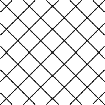
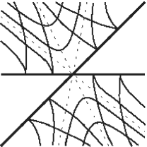
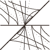
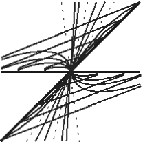
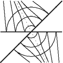
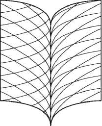
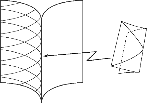
The integral curves of the above BDEs are in Figures 1, 2, 3 which are taken from [5].

Refer to caption
Refer to caption
Figure 1: Integral curves of $\omega_{reg}$ and Ο‰c​u​s​psubscriptπœ”π‘π‘’π‘ π‘\omega_{cusp}.
Refer to caption
Refer to caption
Refer to caption
Figure 2: Integral curves of $\omega_{3s}$, $\omega_{2s1n}$ and $\omega_{1s2n}$. Here and in the rest of the paper, the dashed curves are separatrices, i.e., they are integral curves that separate distinct topological sectors.
Refer to caption
Refer to caption
Figure 3: Integral curves of $\omega_{1s}$ and $\omega_{1n}$.

3 Geometric binary differential equations on a cuspidal edge

Let $f:(\boldsymbol{R}^{2},0)\to(\boldsymbol{R}^{3},0)$ be a parametrization of a cuspidal edge. We take $f$ as in (1.2). Then the coefficients of the first fundamental form of the cuspidal edge with respect to $f$ are

$$\begin{array}[]{rcl}E&=&1+(a_{20}^{2}+b_{20}^{2})u^{2}+(a_{20}a_{30}+b_{20}b_{30})u^{3}+b_{12}b_{20}uv^{2}\\[5.69054pt] &&+\dfrac{1}{4}\Big{(}a_{30}^{2}+b_{30}^{2}+2a_{20}p(0)+2b_{20}q_{1}(0)\Big{)}u^{4}\\[8.53581pt] &&+\dfrac{1}{2}\Big{(}b_{12}b_{30}+8b_{20}q_{2}(0)\Big{)}u^{2}v^{2}+2b_{20}q_{3}(0)uv^{3}\\[8.53581pt] &&+\dfrac{1}{4}b_{12}^{2}v^{4}+O(5),\end{array}$$ (3.1)
$$\begin{array}[]{rcl}F&=&a_{20}uv+\left(\dfrac{1}{2}a_{30}+b_{12}b_{20}\right)u^{2}v+\dfrac{1}{2}b_{03}b_{20}uv^{2}\\[8.53581pt] &&+\dfrac{1}{4}b_{03}b_{12}v^{4}+\left(\dfrac{1}{2}b_{12}^{2}+4b_{20}q_{4}(0,0)\right)uv^{3}\\[8.53581pt] &&+\dfrac{1}{4}\Big{(}b_{03}b_{30}+12b_{20}q_{3}(0)\Big{)}u^{2}v^{2}\\[8.53581pt] &&+\left(\dfrac{1}{2}b_{12}b_{30}+4p(0)+2b_{20}q_{2}(0)\right)u^{3}v+O(5),\\[8.53581pt] \end{array}$$ (3.2)
$$\begin{array}[]{rcl}G&=&v^{2}+\dfrac{1}{4}b_{03}^{2}v^{4}+b_{03}b_{12}uv^{3}+b_{12}^{2}u^{2}v^{2}+O(5),\end{array}$$ (3.3)

where $O(n)$ stands for remainders of order $n$ $(n=1,2,\ldots)$. Since $f$ is as in (1.2), we see fuΓ—(fv/v)β‰ 0subscript𝑓𝑒subscript𝑓𝑣𝑣0f_{u}\times(f_{v}/v)\neq 0. We set $\nu_{2}=f_{u}\times(f_{v}/v)$, and $L_{2}=\left\langle{f_{uu}},{\nu_{2}}\right\rangle$, $M_{2}=\left\langle{f_{uv}},{\nu_{2}}\right\rangle$, $N_{2}=\left\langle{f_{vv}},{\nu_{2}}\right\rangle$. Then we have:

$$\begin{array}[]{rcl}L_{2}&=&b_{20}+(b_{30}-a_{20}b_{12})u-\dfrac{1}{2}a_{20}b_{03}v\\[8.53581pt] &&-\big{(}a_{30}b_{12}-12q_{1}(0)+2a_{20}q_{2}(0)\big{)}u^{2}\\[5.69054pt] &&-\big{(}a_{30}b_{03}+6a_{20}q_{3}(0)\big{)}uv\\[5.69054pt] &&+\big{(}2q_{2}(0)-4a_{20}q_{4}(0,0)\big{)}v^{2}+O(3)\\[5.69054pt] M_{2}&=&b_{12}v+4q_{2}(0)uv+3q_{3}(0)v^{2}+O(3)\\[5.69054pt] N_{2}&=&\dfrac{1}{2}b_{03}v+3q_{3}(0)uv+8q_{4}(0,0)v^{2}+O(3).\end{array}$$ (3.4)

We have $L_{2}=L|\nu_{2}|$, $M_{2}=M|\nu_{2}|$, $N_{2}=N|\nu_{2}|$. It should be remarked that there exist $C^{\infty}$-functions $\widetilde{F},\widetilde{G},\widetilde{N},\widetilde{M}$ such that $G=v^{2}\widetilde{G}$, $F=v\widetilde{F}$, $N_{2}=v\widetilde{N}$ and $M_{2}=v\widetilde{M}$ holds. We set

$$\widetilde{E}=E,\ \widetilde{F}=\dfrac{F}{v},\ \widetilde{G}=\dfrac{G}{v^{2}},\ \widetilde{L}=L_{2},\ \widetilde{M}=\dfrac{M_{2}}{v},\ \widetilde{N}=\dfrac{N_{2}}{v}.$$ (3.5)

3.1 Lines of principal curvature

In this subsection we consider the BDE $\omega_{lc}=0$. Using (3.5), $\omega_{lc}=0$ is equivalent to

$$v^{2}\left(\widetilde{F}\widetilde{N}-v\widetilde{G}\widetilde{M}\right)dv^{2}+v\left(\widetilde{E}\widetilde{N}-v^{2}\widetilde{G}\widetilde{L}\right)dudv+v\left(\widetilde{E}\widetilde{M}-\widetilde{F}\widetilde{L}\right)du^{2}=0.$$

To determine the topological configuration of $\omega_{lc}=0$, we factor out $v$ and consider $\widetilde{\omega}_{lc}=0$, where

$$\widetilde{\omega}_{lc}=v\left(\widetilde{F}\widetilde{N}-v\widetilde{G}\widetilde{M}\right)dv^{2}+\left(\widetilde{E}\widetilde{N}-v^{2}\widetilde{G}\widetilde{L}\right)dudv+\left(\widetilde{E}\widetilde{M}-\widetilde{F}\widetilde{L}\right)du^{2}.$$

We have the following proposition.

Proposition 3.1.

The BDE $\widetilde{\omega}_{lc}=0$ is equivalent to the BDE $\omega_{reg}=0$.

This proposition implies that the lines of principal curvature of a cuspidal edge form a pair of smooth and transverse foliations in the domain of a parametrization.

Proof of Proposition 3.1.

Set

$$(a,b,c)=\left(v\widetilde{F}\widetilde{N}-v^{2}\widetilde{G}\widetilde{M},\ \dfrac{1}{2}\Big{(}\widetilde{E}\widetilde{N}-v\widetilde{G}\widetilde{L}\Big{)},\ \widetilde{E}\widetilde{M}-\widetilde{F}\widetilde{L}\right).$$

Then since $b(0)=\widetilde{E}(0)\widetilde{N}(0)$, E~​(0)=⟨fu,fuβŸ©β€‹(0)β‰ 0~𝐸0subscript𝑓𝑒subscript𝑓𝑒00\widetilde{E}(0)=\left\langle{f_{u}},{f_{u}}\right\rangle(0)\neq 0 and N~​(0)=⟨fv​v​v,Ξ½2βŸ©β€‹(0)=b03β‰ 0~𝑁0subscript𝑓𝑣𝑣𝑣subscript𝜈20subscript𝑏030\widetilde{N}(0)=\left\langle{f_{vvv}},{\nu_{2}}\right\rangle(0)=b_{03}\neq 0 hold, $\widetilde{\omega}_{lc}$ is as in Case 1. Moreover, since $a(0)=0$ and b​(0)β‰ 0𝑏00b(0)\neq 0, we see that $b^{2}-ac>0$ at 00. Hence $\widetilde{\omega}_{lc}$ is equivalent to $\omega_{reg}=0$ (See Section 2.1). ∎

The fact of the existence of the curvature line coordinate system at cuspidal edge is also shown in [24].

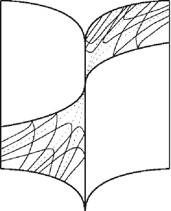
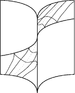
An example of picture of this configuration on the cuspidal edges is in Figures 4. Since one family of the integral curves are tangent to the null direction on singular curve, one family of the integral curves near singular curve form the $(2,3)$-cusps. A map-germ $(\boldsymbol{R},0)\to(\boldsymbol{R}^{3},0)$ is an $(2,3)$-cusp if it is $\mathcal{A}$-equivalent to $t\mapsto(t^{2},t^{3})$.

Refer to caption
Figure 4: Integral curves of $\widetilde{\omega}_{lc}$ on images of cuspidal edges.

3.2 Asymptotic curves

In this subsection we consider Ο‰a​s=0subscriptπœ”π‘Žπ‘ 0\omega_{as}=0, and it is equivalent to Ο‰~a​s=N2​d​v2+2​M2​d​u​d​v+N2​d​u2=0subscript~πœ”π‘Žπ‘ subscript𝑁2𝑑superscript𝑣22subscript𝑀2𝑑𝑒𝑑𝑣subscript𝑁2𝑑superscript𝑒20\widetilde{\omega}_{as}=N_{2}\,dv^{2}+2M_{2}\,dudv+N_{2}\,du^{2}=0. Since $M_{2}(u,0)=0$, and $N_{2}(u,0)=0$, the singular set i.e., the cuspidal edge curve is part of discriminant of Ο‰~a​s=0subscript~πœ”π‘Žπ‘ 0\widetilde{\omega}_{as}=0, and, $\partial_{v}$ is a solution to Ο‰~a​s=0subscript~πœ”π‘Žπ‘ 0\widetilde{\omega}_{as}=0 on the singular set. By (3.4),

$$\begin{array}[]{rcl}\displaystyle\delta(u,v)&=&\displaystyle-\dfrac{1}{2}b_{20}b_{03}v+\left(\frac{1}{4}a_{20}b_{03}^{2}+b_{12}^{2}-8b_{20}q_{4}(0,0)\right)v^{2}\\[8.53581pt] &&+\dfrac{1}{2}b_{03}\Big{(}a_{20}b_{12}-b_{30}-2b_{20}q_{3}(0)\Big{)}uv\\[8.53581pt] &&\displaystyle+\Big{(}-b_{03}q_{2}(0)+6b_{12}q_{3}(0)\\[8.53581pt] &&\displaystyle\hskip 42.67912pt+6a_{20}b_{03}q_{4}(0,0)-7b_{20}(q_{4})_{v}(0,0)\Big{)}v^{3}\\[8.53581pt] &&\displaystyle+\Bigg{(}\frac{1}{4}a_{30}b_{03}^{2}+3a_{20}b_{03}q_{3}(0)-8b_{30}q_{4}(0,0)\\[8.53581pt] &&\hskip 42.67912pt+8b_{12}q_{2}(0)+8a_{20}b_{12}q_{4}(0,0)\Bigg{)}uv^{2}\\[8.53581pt] &&\displaystyle+\Bigg{(}\frac{1}{2}a_{30}b_{03}b_{12}-6b_{03}q_{1}(0)+a_{20}b_{03}q_{2}(0)\\[8.53581pt] &&\hskip 42.67912pt+3a_{20}b_{12}q_{3}(0)-3b_{30}q_{3}(0)\Bigg{)}u^{2}v+O(4).\end{array}$$ (3.6)

Thus if b20β‰ 0subscript𝑏200b_{20}\neq 0, then the BDE is in Case 2. In this case, by (3.4), Ο‰a​s=0subscriptπœ”π‘Žπ‘ 0\omega_{as}=0 is equivalent to Ο‰c​u​s​p=0subscriptπœ”π‘π‘’π‘ π‘0\omega_{cusp}=0 (see Subsection 2.2). By [28, Corollary 3.6], b20β‰ 0subscript𝑏200b_{20}\neq 0 implies that the Gaussian curvature is unbounded and changes sign between the two sides of the cuspidal edge. This means that in this case, the singular set of cuspidal edge plays the same role as the parabolic curve on regular surfaces. Since b20β‰ 0subscript𝑏200b_{20}\neq 0, then the BDE is Ο‰c​u​s​p=0subscriptπœ”π‘π‘’π‘ π‘0\omega_{cusp}=0, this implies that the folded saddle, the folded node, the folded focus in Davydov’s classification [9] (see also [30, Section 3.2]) does not appear not only cuspidal edges, but also all singularities written in the form (1.1) (for instance, cuspidal cross cap).

We assume now $b_{20}=0$. Then the BDE is in Case 3. We have the following. If a20​b12βˆ’b30β‰ 0subscriptπ‘Ž20subscript𝑏12subscript𝑏300a_{20}b_{12}-b_{30}\neq 0, then $\delta$ is a Morse function near 00. We study the geometric foliation near 00 as in Subsection 2.3. We consider

$$\mathcal{F}(u,v,p)=N_{2}+2M_{2}p+L_{2}p^{2}.$$

Then we have

$$\begin{array}[]{rcl}(\mathcal{F}_{u},\mathcal{F}_{v},\mathcal{F}_{p})(u,v,p)&=&\big{(}(N_{2})_{u}+2(M_{2})_{u}p+(L_{2})_{u}p^{2},\\ &&(N_{2})_{v}+2(M_{2})_{v}p+(L_{2})_{v}p^{2},2M_{2}+2L_{2}p\big{)},\\ (\mathcal{F}_{u},\mathcal{F}_{v},\mathcal{F}_{p})(0,0,p)&=&\big{(}(L_{2})_{u}p^{2},(N_{2})_{v}+2(M_{2})_{v}p+(L_{2})_{v}p^{2},2Lp\big{)}\\ &=&\left(\big{(}b_{30}-a_{20}b_{12}\big{)}p^{2},\dfrac{1}{2}\big{(}b_{03}+4b_{12}p-a_{20}b_{03}p^{2}\big{)},0\right).\end{array}$$

In this case, the left hand side of (2.1) is $(b_{30}-a_{20}b_{12})^{2}b_{03}^{2}/4$. Thus if b30βˆ’a20​b12β‰ 0subscript𝑏30subscriptπ‘Ž20subscript𝑏120b_{30}-a_{20}b_{12}\neq 0 at 00, then $\mathcal{M}=\{\mathcal{F}=0\}$ is a smooth manifold. We have Ο†a​s=φωa​ssubscriptπœ‘π‘Žπ‘ subscriptπœ‘subscriptπœ”π‘Žπ‘ \varphi_{as}=\varphi_{\omega_{as}} and Da​s=DΟ‰a​ssubscriptπ·π‘Žπ‘ subscript𝐷subscriptπœ”π‘Žπ‘ D_{as}=D_{\omega_{as}} defined in Subsection 2.3 as follows

Ο†a​s​(p)=(b30βˆ’a20​b12)​p3βˆ’12​a20​b03​p2+2​b12​p+12​b03,4​Da​s=a203​b034+13​a202​b032​b122βˆ’b30​(128​b123+27​b032​b30)+2​a20​(64​b124+9​b032​b12​b30).subscriptπœ‘π‘Žπ‘ π‘subscript𝑏30subscriptπ‘Ž20subscript𝑏12superscript𝑝312subscriptπ‘Ž20subscript𝑏03superscript𝑝22subscript𝑏12𝑝12subscript𝑏034subscriptπ·π‘Žπ‘ superscriptsubscriptπ‘Ž203superscriptsubscript𝑏03413superscriptsubscriptπ‘Ž202superscriptsubscript𝑏032superscriptsubscript𝑏122subscript𝑏30128superscriptsubscript𝑏12327superscriptsubscript𝑏032subscript𝑏30missing-subexpressionmissing-subexpression2subscriptπ‘Ž2064superscriptsubscript𝑏1249superscriptsubscript𝑏032subscript𝑏12subscript𝑏30\begin{array}[]{rcL}\varphi_{as}(p)&=&(b_{30}-a_{20}b_{12})p^{3}-\frac{1}{2}a_{20}b_{03}p^{2}+2b_{12}p+\frac{1}{2}b_{03},\\[5.69054pt] 4D_{as}&=&a_{20}^{3}b_{03}^{4}+13a_{20}^{2}b_{03}^{2}b_{12}^{2}-b_{30}(128b_{12}^{3}+27b_{03}^{2}b_{30})\\ &&+2a_{20}(64b_{12}^{4}+9b_{03}^{2}b_{12}b_{30}).\end{array}

Furthermore, $\alpha(p)$ is given by

$$\alpha(p)=2(b_{30}-a_{20}b_{12})p^{2}-a_{20}b_{03}p+2b_{12}.$$

If $p_{i}$ is a solution of Ο†a​s​(p)=0subscriptπœ‘π‘Žπ‘ π‘0\varphi_{as}(p)=0 and p​α​(p)βˆ’2​φa​s​(p)=βˆ’b03βˆ’2​b12​p𝑝𝛼𝑝2subscriptπœ‘π‘Žπ‘ π‘subscript𝑏032subscript𝑏12𝑝p\alpha(p)-2\varphi_{as}(p)=-b_{03}-2b_{12}p holds, then α​(pi)β‰ 0𝛼subscript𝑝𝑖0\alpha(p_{i})\neq 0 if and only if βˆ’b03βˆ’2​b12​piβ‰ 0subscript𝑏032subscript𝑏12subscript𝑝𝑖0-b_{03}-2b_{12}p_{i}\neq 0. Assume that b12β‰ 0subscript𝑏120b_{12}\neq 0. Substituting $p=-b_{03}/(2b_{12})$ into Ο†a​s​(p)subscriptπœ‘π‘Žπ‘ π‘\varphi_{as}(p), we get

Ο†a​s​(βˆ’b032​b12)=βˆ’18​b123​b03​(4+b032​b30).subscriptπœ‘π‘Žπ‘ subscript𝑏032subscript𝑏1218superscriptsubscript𝑏123subscript𝑏034superscriptsubscript𝑏032subscript𝑏30\varphi_{as}\left(\dfrac{-b_{03}}{2b_{12}}\right)=-\dfrac{1}{8b_{12}^{3}}b_{03}\big{(}4+b_{03}^{2}b_{30}\big{)}.

If $b_{12}=0$, then p​α​(p)βˆ’2​φa​s​(p)=βˆ’b03β‰ 0𝑝𝛼𝑝2subscriptπœ‘π‘Žπ‘ π‘subscript𝑏030p\alpha(p)-2\varphi_{as}(p)=-b_{03}\neq 0. Since we assume that b30βˆ’a20​b12β‰ 0subscript𝑏30subscriptπ‘Ž20subscript𝑏120b_{30}-a_{20}b_{12}\neq 0, if $b_{12}=0$ then b30β‰ 0subscript𝑏300b_{30}\neq 0. Thus we get α​(pi)β‰ 0𝛼subscript𝑝𝑖0\alpha(p_{i})\neq 0 if and only if

4​b123+b032​b30β‰ 0.4superscriptsubscript𝑏123superscriptsubscript𝑏032subscript𝑏3004b_{12}^{3}+b_{03}^{2}b_{30}\neq 0.

We can now use Theorem 2.3 to obtain the following result.

Proposition 3.2.

If b20β‰ 0subscript𝑏200b_{20}\neq 0, then Ο‰a​ssubscriptπœ”π‘Žπ‘ \omega_{as} is equivalent to Ο‰c​u​s​p=0subscriptπœ”π‘π‘’π‘ π‘0\omega_{cusp}=0.

If $b_{20}=0$, b30βˆ’a20​b12β‰ 0subscript𝑏30subscriptπ‘Ž20subscript𝑏120b_{30}-a_{20}b_{12}\neq 0, Da​sβ‰ 0subscriptπ·π‘Žπ‘ 0D_{as}\neq 0 and 4​b123+b032​b30β‰ 04superscriptsubscript𝑏123superscriptsubscript𝑏032subscript𝑏3004b_{12}^{3}+b_{03}^{2}b_{30}\neq 0, then Ο‰a​ssubscriptπœ”π‘Žπ‘ \omega_{as} is topologically equivalent to one of the following$:$

  • β€’

    The case Da​s>0subscriptπ·π‘Žπ‘ 0D_{as}>0 : $($Then Ο†a​s​(p)=0subscriptπœ‘π‘Žπ‘ π‘0\varphi_{as}(p)=0 has $3$ roots $p_{1},p_{2},p_{3})$

    • –

      Ο‰3​ssubscriptπœ”3𝑠\omega_{3s} $($βˆ’Ο†a​s′​(pi)​α​(pi)superscriptsubscriptπœ‘π‘Žπ‘ β€²subscript𝑝𝑖𝛼subscript𝑝𝑖-\varphi_{as}^{\prime}(p_{i})\alpha(p_{i}) are negative for all $i=1,2,3)$.

    • –

      Ο‰2​s​1​nsubscriptπœ”2𝑠1𝑛\omega_{2s1n} $($βˆ’Ο†a​s′​(pi)​α​(pi)superscriptsubscriptπœ‘π‘Žπ‘ β€²subscript𝑝𝑖𝛼subscript𝑝𝑖-\varphi_{as}^{\prime}(p_{i})\alpha(p_{i}) are two negative and one positive for $i=1,2,3)$.

    • –

      Ο‰1​s​2​nsubscriptπœ”1𝑠2𝑛\omega_{1s2n} $($βˆ’Ο†a​s′​(pi)​α​(pi)superscriptsubscriptπœ‘π‘Žπ‘ β€²subscript𝑝𝑖𝛼subscript𝑝𝑖-\varphi_{as}^{\prime}(p_{i})\alpha(p_{i}) are one negative and two positive for $i=1,2,3)$.

  • β€’

    The case Da​s<0subscriptπ·π‘Žπ‘ 0D_{as}<0 : $($Then Ο†a​s​(p)=0subscriptπœ‘π‘Žπ‘ π‘0\varphi_{as}(p)=0 has $1$ root $p_{1})$

    • –

      Ο‰1​ssubscriptπœ”1𝑠\omega_{1s} $($βˆ’Ο†a​s′​(p1)​α​(p1)superscriptsubscriptπœ‘π‘Žπ‘ β€²subscript𝑝1𝛼subscript𝑝1-\varphi_{as}^{\prime}(p_{1})\alpha(p_{1}) is negative$)$.

    • –

      Ο‰1​nsubscriptπœ”1𝑛\omega_{1n} $($βˆ’Ο†a​s′​(p1)​α​(p1)superscriptsubscriptπœ‘π‘Žπ‘ β€²subscript𝑝1𝛼subscript𝑝1-\varphi_{as}^{\prime}(p_{1})\alpha(p_{1}) is positive$)$.

Remark 3.3.

We observe that by the Proposition 3.2, $b_{20}$, $b_{30}-a_{20}b_{12}$ and $4b_{12}^{3}+b_{03}^{2}b_{30}$ have geometric meanings. In fact, $b_{20}$ is the limiting normal curvature and $b_{30}-a_{20}b_{12}$ coincides with the derivation of limiting normal curvature (see [23]). The invariant $4b_{12}^{3}+b_{03}^{2}b_{30}$ is related to the singularities of parallel surfaces of the cuspidal edge (see [31, Lemma 3.1]).

3.3 Characteristic curves

We consider the BDE $\omega_{ch}=0$. Using (3.5), we show that $\omega_{ch}=0$ is equivalent to $v(a\,dv^{2}+2b\,dudv+c\,du^{2})=0$, where

$$\begin{array}[]{rcL}a&=&v\Big{(}\widetilde{E}\widetilde{N}^{2}+\big{(}-\widetilde{G}\widetilde{L}\widetilde{N}-2\widetilde{F}\widetilde{M}\widetilde{N}\big{)}v+2\widetilde{G}\widetilde{M}^{2}v^{2}\Big{)}\\ b&=&v\big{(}-2\widetilde{F}\widetilde{L}\widetilde{N}+\widetilde{E}\widetilde{M}\widetilde{N}+\widetilde{G}\widetilde{L}\widetilde{M}v\big{)}\\ c&=&-\widetilde{E}\widetilde{L}\widetilde{N}+\big{(}\widetilde{G}\widetilde{L}^{2}-2\widetilde{F}\widetilde{L}\widetilde{M}+2\widetilde{E}\widetilde{M}^{2}\big{)}v.\end{array}$$

We factor out $v$, so $\omega_{ch}=0$ is topologically equivalent to $\tilde{\omega}_{ch}=a\,dv^{2}+2b\,dudv+c\,du^{2}=0$. Since $a(u,0)=0$, and $b(u,0)=0$, the singular set is a part of discriminant of $\tilde{\omega}_{ch}=0$, and $\partial_{v}$ is a solution to $\tilde{\omega}_{ch}=0$ on the singular set. The function $\delta=b^{2}-ac$ is given by

$$\begin{array}[]{l}v\Big{[}\widetilde{E}^{2}\widetilde{L}\widetilde{N}^{3}+\big{(}4\widetilde{F}^{2}\widetilde{L}^{2}-2\widetilde{E}\widetilde{G}\widetilde{L}^{2}-4\widetilde{E}\widetilde{F}\widetilde{L}\widetilde{M}-2\widetilde{E}^{2}\widetilde{M}^{2}\big{)}\widetilde{N}^{2}v\\ \hskip 14.22636pt+\big{(}-\widetilde{G}^{2}\widetilde{L}^{3}-4\widetilde{F}\widetilde{G}\widetilde{L}^{2}\widetilde{M}-4\widetilde{F}^{2}\widetilde{L}\widetilde{M}^{2}+6\widetilde{E}\widetilde{G}\widetilde{L}\widetilde{M}^{2}+4\widetilde{E}\widetilde{F}\widetilde{M}^{3}\big{)}\widetilde{N}v^{2}\\ \hskip 28.45274pt+\big{(}\widetilde{G}\widetilde{L}^{2}-4\widetilde{F}\widetilde{L}\widetilde{M}+4\widetilde{E}\widetilde{M}^{2}\big{)}\widetilde{G}\widetilde{M}^{2}v^{3}\Big{]}.\end{array}$$

When $f$ is taken as in (1.2), we have

$$\begin{array}[]{RcL}a&=&\frac{1}{4}b_{03}^{2}v+O(2),\\[5.69054pt] b&=&\frac{1}{2}b_{12}b_{03}v+O(2),\\[5.69054pt] c&=&-\frac{1}{2}b_{20}b_{03}+\frac{1}{2}\big{(}a_{20}b_{12}b_{03}-b_{30}b_{03}-6b_{20}q_{3}(0)\big{)}u\\[5.69054pt] \hfil&&\hskip 28.45274pt+\frac{1}{4}\Big{[}a_{20}b_{03}^{2}+8b_{12}^{2}+4b_{20}\big{(}b_{20}-8q_{4}(0,0)\big{)}\Big{]}v+O(2),\\[5.69054pt] \delta&=&\dfrac{1}{8}b_{03}^{3}b_{20}v+\dfrac{1}{8}b_{03}^{2}\big{(}-a_{20}b_{03}b_{12}+b_{03}b_{30}+18b_{20}q_{3}(0)\big{)}uv\\[5.69054pt] \hfil&&\hskip 2.84526pt-\dfrac{1}{16}b_{03}^{2}\bigg{[}a_{20}b_{03}^{2}+4\Big{[}b_{12}^{2}+2b_{20}\big{(}b_{20}-12q_{4}(0,0)\big{)}\Big{]}\bigg{]}v^{2}+O(3).\end{array}$$

Since b03β‰ 0subscript𝑏030b_{03}\neq 0, if b20β‰ 0subscript𝑏200b_{20}\neq 0, then $\widetilde{\omega}_{ch}$ is as in Case 2, and if $b_{20}=0$, then it is as in Case 3. In the following, we divide our consideration into these two cases.

The case b20β‰ 0subscript𝑏200b_{20}\neq 0 :

By the argument in Subsection 2.2, $\widetilde{\omega}_{ch}=0$ is equivalent to Ο‰c​u​s​p=0subscriptπœ”π‘π‘’π‘ π‘0\omega_{cusp}=0. In this case, by (3.4), Ο‰a​s=0subscriptπœ”π‘Žπ‘ 0\omega_{as}=0 is equivalent to Ο‰c​u​s​p=0subscriptπœ”π‘π‘’π‘ π‘0\omega_{cusp}=0 (see Subsection 2.2). Like as the case of Ο‰a​s=0subscriptπœ”π‘Žπ‘ 0\omega_{as}=0, the singular set of cuspidal edge plays the same role as the parabolic curve on regular surfaces. Moreover, the folded saddle, the folded node, the folded focus do not appear.

The case $b_{20}=0$ :

The left hand side of (2.1) is $b_{03}^{6}(a_{20}b_{12}-b_{30})^{2}/64$. Thus $\mathcal{M}$ is a smooth manifold if a20​b12βˆ’b30β‰ 0subscriptπ‘Ž20subscript𝑏12subscript𝑏300a_{20}b_{12}-b_{30}\neq 0 at 00. Furthermore, $\delta$ is of Morse type if and only if a20​b12βˆ’b30β‰ 0subscriptπ‘Ž20subscript𝑏12subscript𝑏300a_{20}b_{12}-b_{30}\neq 0. This is exactly the same conditions as the case of asymptotic curves. We assume that a20​b12βˆ’b30β‰ 0subscriptπ‘Ž20subscript𝑏12subscript𝑏300a_{20}b_{12}-b_{30}\neq 0. We need to consider $\mathcal{F}(u,v,p)=a+2bp+cp^{2}$ and $\varphi_{ch}(p)=(p\mathcal{F}_{u}+\mathcal{F}_{v})(0,0,p)$. We have

$$\begin{array}[]{l}4\varphi_{ch}(p)=b_{03}^{2}+4b_{03}b_{12}p\\ \hskip 51.21495pt+(a_{20}b_{03}^{2}+8b_{12}^{2})p^{2}+(2a_{20}b_{03}b_{12}-2b_{03}b_{30})p^{3},\end{array}$$ (3.7)

and the discriminant $D_{ch}=D_{\omega_{ch}}$ of the cubic $\varphi_{ch}$ is given by

$$\begin{array}[]{L}D_{ch}=-\dfrac{b_{03}^{2}}{64}\Big{(}a_{20}^{3}b_{03}^{6}+11a_{20}^{2}b_{03}^{4}b_{12}^{2}\\ \hskip 56.9055pt-2a_{20}(16b_{03}^{2}b_{12}^{4}+9b_{03}^{4}b_{12}b_{30})\\ \hskip 113.81102pt+256b_{12}^{6}+160b_{03}^{2}b_{12}^{3}b_{30}+27b_{03}^{4}b_{30}^{2}\Big{)}.\end{array}$$ (3.8)

Furthermore, $4\alpha$ is given by

$$4\alpha(p)=2b_{03}(a_{20}b_{12}-b_{30})p^{2}+(a_{20}b_{03}^{2}+8b_{12}^{2})p+2b_{12}b_{03}.$$

Then we have

$$\begin{array}[]{l}4\varphi_{ch}^{\prime}(p)\alpha(p)=4b_{03}^{2}b_{12}^{2}+4b_{03}b_{12}(a_{20}b_{03}^{2}+8b_{12}^{2})p\\ \hskip 62.59605pt+(a_{20}^{2}b_{03}^{4}+26a_{20}b_{03}^{2}b_{12}^{2}+64b_{12}^{4}-10b_{03}^{2}b_{12}b_{30})p^{2}\\ \hskip 62.59605pt+5b_{03}(a_{20}b_{03}^{2}+8b_{12}^{2})(a_{20}b_{12}-b_{30})p^{3}\\ \hskip 62.59605pt+6b_{03}^{2}(-a_{20}b_{12}+b_{30})^{2}p^{4},\end{array}$$ (3.9)

and the condition that $\varphi_{ch}(p)$ and $\alpha(p)$ do not have any common roots is given by 4​b123+b032​b30β‰ 04superscriptsubscript𝑏123superscriptsubscript𝑏032subscript𝑏3004b_{12}^{3}+b_{03}^{2}b_{30}\neq 0. We summerize the above discussion in the following proposition.

Proposition 3.4.

If b20β‰ 0subscript𝑏200b_{20}\neq 0, then $\omega_{ch}$ is equivalent to Ο‰c​u​s​p=0subscriptπœ”π‘π‘’π‘ π‘0\omega_{cusp}=0.

If $b_{20}=0$, b30βˆ’a20​b12β‰ 0subscript𝑏30subscriptπ‘Ž20subscript𝑏120b_{30}-a_{20}b_{12}\neq 0, Dc​hβ‰ 0subscriptπ·π‘β„Ž0D_{ch}\neq 0 and 4​b123+b032​b30β‰ 04superscriptsubscript𝑏123superscriptsubscript𝑏032subscript𝑏3004b_{12}^{3}+b_{03}^{2}b_{30}\neq 0, then $\omega_{ch}$ is topologically equivalent to one of the following:

  • β€’

    The case $D_{ch}>0$ : $($Then $\varphi_{ch}(p)=0$ has $3$ roots $p_{1},p_{2},p_{3})$

    • –

      Ο‰3​ssubscriptπœ”3𝑠\omega_{3s} $($ $-\varphi_{ch}^{\prime}(p_{i})\alpha(p_{i})$ are negative for all $i=1,2,3)$.

    • –

      Ο‰2​s​1​nsubscriptπœ”2𝑠1𝑛\omega_{2s1n} $($ $-\varphi_{ch}^{\prime}(p_{i})\alpha(p_{i})$ are two negative and one positive for $i=1,2,3)$.

    • –

      Ο‰1​s​2​nsubscriptπœ”1𝑠2𝑛\omega_{1s2n} $($ $-\varphi_{ch}^{\prime}(p_{i})\alpha(p_{i})$ are one negative and two positive for $i=1,2,3)$.

  • β€’

    The case $D_{ch}<0$ : $($Then $\varphi_{ch}(p)=0$ has $1$ root $p_{1})$

    • –

      Ο‰1​ssubscriptπœ”1𝑠\omega_{1s} $($ $-\varphi_{ch}^{\prime}(p_{1})\alpha(p_{1})$ is negative$)$.

    • –

      Ο‰1​nsubscriptπœ”1𝑛\omega_{1n} $($ $-\varphi_{ch}^{\prime}(p_{1})\alpha(p_{1})$ is positive$)$.

Remark 3.5.

We remark that if $b_{12}=0$, then Da​s=Dc​hsubscriptπ·π‘Žπ‘ subscriptπ·π‘β„ŽD_{as}=D_{ch}. Namely, the configrations of foliations with respect to Ο‰a​ssubscriptπœ”π‘Žπ‘ \omega_{as} and $\omega_{ch}$ are of the same type.

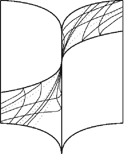
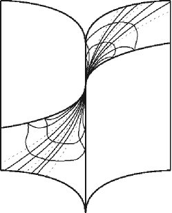
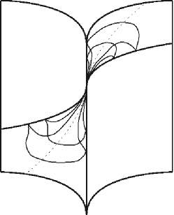
Examples of pictures of these configrations on the cuspidal edges are in Figures 5, 6 and 7. Since the integral curves emanate from singular curve along the null direction, integral curves near the singular curve do not form the $(2,3)$-cusp but form the $(3,4)$-cusps (see Appendix A).

Refer to caption
Figure 5: Integral curves of Ο‰c​u​s​psubscriptπœ”π‘π‘’π‘ π‘\omega_{cusp} on images of cuspidal edges.
Refer to caption
Refer to caption
Refer to caption
Figure 6: Integral curves of $\omega_{3s}$, $\omega_{2s1n}$ and $\omega_{1s2n}$ on images of cuspidal edges.
Refer to caption
Refer to caption
Figure 7: Integral curves of $\omega_{1s}$ and $\omega_{1n}$ on images of cuspidal edges.

4 Generic foliations

In Propositions 3.2 and 3.4, all the conditions are written in terms of the $3$-jet of (1.2). We can state a genericity result for cuspidal edge. By (1.2), we identify the set of jets of parametrization of cuspidal edges with $(0,0)$

π’žk={(jka1(0),jkb2(0),jkb3(0),jkb4(0,0))∈Jk(1,1)3Γ—Jk(2,1)|a1(0)=a1β€²(0)=b2(0)=b2β€²(0)=b3(0)=0,b2β€²(0)>0,b4(0,0)β‰ 0},\begin{array}[]{l}\mathcal{C}_{k}=\Big{\{}\big{(}j^{k}a_{1}(0),j^{k}b_{2}(0),j^{k}b_{3}(0),j^{k}b_{4}(0,0)\big{)}\in J^{k}(1,1)^{3}\times J^{k}(2,1)\,\Big{|}\\[11.38109pt] a_{1}(0)=a_{1}^{\prime}(0)=b_{2}(0)=b_{2}^{\prime}(0)=b_{3}(0)=0,\ b_{2}^{\prime}(0)>0,\ b_{4}(0,0)\neq 0\Big{\}},\end{array}

for $k\geq 3$. With notation as before, consider

$$(a_{20},a_{30},\ldots,b_{20},b_{30},\ldots,b_{12},\ldots,b_{03},\ldots)$$

as a coordinate system of $\mathcal{C}_{k}$ (cf. (1.2)). Define a subset of $\mathcal{C}_{k}$ by

𝒩={b20=0,b30βˆ’a20​b12=0}βˆͺ{b20=0,Da​s​y=0}βˆͺ{b20=0, 4​b123βˆ’b032​b30=0}βˆͺ{b20=0,Dh​m​c=0}.𝒩formulae-sequencesubscript𝑏200subscript𝑏30subscriptπ‘Ž20subscript𝑏120formulae-sequencesubscript𝑏200subscriptπ·π‘Žπ‘ π‘¦0formulae-sequencesubscript𝑏2004superscriptsubscript𝑏123superscriptsubscript𝑏032subscript𝑏300formulae-sequencesubscript𝑏200subscriptπ·β„Žπ‘šπ‘0\begin{array}[]{l}\mathcal{N}=\{b_{20}=0,\ b_{30}-a_{20}b_{12}=0\}\cup\{b_{20}=0,\ D_{asy}=0\}\\ \hskip 28.45274pt\cup\{b_{20}=0,\ 4b_{12}^{3}-b_{03}^{2}b_{30}=0\}\cup\{b_{20}=0,\ D_{hmc}=0\}.\end{array}

Then $\mathcal{N}$ is an algebaric subset of $\mathcal{C}_{k}$ of codimension $2$. Since the singular set of a cuspidal edge is a curve, generically it will avoid the set $\mathcal{N}$. This implies that for generic cuspidal edges the configuration of Ο‰l​c,Ο‰a​s,Ο‰c​hsubscriptπœ”π‘™π‘subscriptπœ”π‘Žπ‘ subscriptπœ”π‘β„Ž\omega_{lc},\omega_{as},\omega_{ch} are those in Propositions 3.1, 3.2, 3.4.

Appendix A Criteria for $(3,4)$ and $(3,4,5)$-cusp

In this section, we state criteria for $(3,4)$ and $(3,4,5)$-cusp. Set

$$c_{1}(t)=(t^{3},t^{4},0,\ldots,0),\quad c_{2}(t)=(t^{3},t^{4},t^{5},0,\ldots,0),$$

and a map-germ $\gamma:(\boldsymbol{R},0)\to(\boldsymbol{R}^{n},0)$, where $n\geq 2$ (respectively, $n\geq 3$) is called $(3,4)$-cusp (respectively, $(3,4,5)$-cusp) if $\gamma$ is $\mathcal{A}$-equivalent to the map-germ $c_{1}$ (respectively, $c_{2}$) at 00.

Proposition A.1.

A map-germ $\gamma:(\boldsymbol{R},0)\to(\boldsymbol{R}^{n},0)$, where $n\geq 3$ $($respectively, $n\geq 2)$ is $(3,4,5)$-cusp $($respectively, $(3,4)$-cusp$)$ if and only if

  • (i)

    $\gamma^{\prime}(0)=\gamma^{\prime\prime}(0)=0$,

  • (ii)

    $\gamma^{(3)}(0),\gamma^{(4)}(0)$ and $\gamma^{(5)}(0)$ are linearly independent $($respectively, linearly dependent, and $\gamma^{(3)}(0)$ and $\gamma^{(4)}(0)$ are linearly independent$)$ where $(~{})^{(i)}=d^{i}/dt^{i}$.

Although this proposition is known [4, 14], we give a sketch of proof for the readers who are not familiar with it.

Proof.

Since

$$\Phi(\gamma(t))^{(i)}=d\Phi_{0}(\gamma^{(i)}(0))\quad(i=3,4,5)$$

holds for a map $\Phi:(\boldsymbol{R}^{n},0)\to(\boldsymbol{R}^{n},0)$ under the assumption $\gamma^{\prime}(0)=\gamma^{\prime\prime}(0)=0$, it is obvious that the conditions do not depend on the parameter and the coordinate system on $\boldsymbol{R}^{n}$.

To show the proposition, it is enough to show that $(t^{3}+a_{1}t^{5},t^{4}+a_{2}t^{5},a_{3}t^{5},0,\ldots,0)+O(6)$ is $\mathcal{A}$-equivalent to $(t^{3},t^{4},a_{3}t^{5},0,\ldots,0)+O(6)$, where $a_{1},a_{2},a_{3}\in\boldsymbol{R}$. Considering the parameter change $t\mapsto t-a_{2}t^{2}/4-(16a_{1}+3a_{2}^{2})t^{3}/48,$ it can be proved. ∎

Using Proposition A.1, we have the following:

Proposition A.2.

Let $f:(\boldsymbol{R}^{2},0)\to(\boldsymbol{R}^{3},0)$ be a cuspidal edge and $\gamma:(\boldsymbol{R},0)\to(\boldsymbol{R}^{2},0)$ an ordinary cusp such that $df_{0}(\gamma^{\prime\prime}(0))=0$. Then $\hat{\gamma}=f\circ\gamma$ is a $(3,4)$-cusp at 00.

Proof.

Without loss of generality, one can assume that $f$ is given by the form (1.2), and $\gamma(t)=(t^{3}+a_{4}t^{4}+a_{5}t^{5}+O(6),t^{2})$ $(a_{4},a_{5}\in\boldsymbol{R})$, because $df_{0}(\partial v)=0$. Then $\hat{\gamma}(t)=(t^{3}+a_{4}t^{4}+a_{5}t^{5},t^{4}/2,0)+O(6)$. By Proposition A.1, we have the conclusion. ∎

References

  • [1] V. I. Arnol’d, S. M. Gusein-Zade and A. N. Varchenko, Singularities of differentiable maps, Vol. $1$, Monogr. Math. 82, BirkhΓ€user Boston, Inc., Boston, MA, 1985.
  • [2] J. W. Bruce and , D. L. Fidal, On binary differential equations and umbilics, Proc. Roy. Soc. Edinburgh Sect. A 111 (1989), no. 1-2, 147–168.
  • [3] J. W. Bruce, G. J. Fletcher and F. Tari, Bifurcations of implicit differential equations, Proc. Roy. Soc. Edinburgh Sect. A 130 (2000), no. 3, 485–506.
  • [4] J. W. Bruce and T. J. Gaffney, Simple singularities of mappings $\boldsymbol{C},0\to\boldsymbol{C}^{2},0$, J. London Math. Soc. (2) 26 (1982), no. 3, 465–474.
  • [5] J. W. Bruce and F. Tari, On binary differential equations, Nonlinearity 8 (1995), 255–271.
  • [6] J. W. Bruce and F. Tari, Implicit differential equations from the singularity theory viewpoint, Banach Center Publ. 33 (1996), 23–38.
  • [7] M. Cibrario, Sulla reduzione a forma delle equationi lineari alle derviate parziale di secondo ordine di tipo misto, Accademia di Scienze e Lettere, Instituto Lombardo Redicconti 65 (1932), 889–906.
  • [8] L. Dara, SingularitΓ©s gΓ©nΓ©riques des Γ©quations differentielles multiformes, Bol. Soc. Brasil Math. 6 (1975), 95–128.
  • [9] A. A. Davydov, Normal forms of differential equations unresolved with respect to derivatives in a neighbourhood of its singular point, Functional Anal. Appl. 19 (1985), 1–10.
  • [10] A. A. Davydov, Qualitative Theory of Control Systems, Translations of Mathematical Monographs 142, American Mathematical Society, Providence, R.I. Moscow 1994.
  • [11] A. A. Davydov, G. Ishikawa, S. Izumiya and W. Sun, Generic singularities of implicit systems of first order differential equations on the plane, Jpn. J. Math. 3 (2008), no. 1, 93–119.
  • [12] R. Garcia, C. Gutierrez, and J. Sotomayor, Lines of principal curvature around umbilics and Whitney umbrellas, Tohoku Math.Β J., 52 (2000), 163–172.
  • [13] R. Garcia and J Sotomayor, Harmonic mean curvature lines on surfaces immersed in $\boldsymbol{R}^{3}$, Bull. Braz. Math. Soc. 34 (2003), 303–331.
  • [14] C. G. Gibson and C. A. Hobbs, Simple singularities of space curves, Math. Proc. Cambridge Philos. Soc. 113 (1993), no. 2, 297–310.
  • [15] V. GuΓ­Γ±ez, Positive quadratic differential forms and foliations with singularities on surfaces, Trans. Amer. Math. Soc. 309 (1988), 477-502.
  • [16] V. GuΓ­Γ±ez, Locally stable singularities for positive quadratic differential forms, J. Differential Equations 110 (1994), no. 1, 1–37.
  • [17] V. GuΓ­Γ±ez, C. Gutierrez, Rank $1$ codimension one singularities of positive quadratic differential forms, J. Differential Equations 206 (2004), no. 1, 127–155.
  • [18] A. Hayakawa, G. Ishikawa, S. Izumiya and K. Yamaguchi, Classification of generic integral diagrams and first order ordinary differential equations, Internat. J. Math. 5 (1994), no. 4, 447–489.
  • [19] S. Izumiya and F. Tari, Apparent contours in Minkowski $3$-space and first order ordinary differential equations, Nonlinearity 26 (2013), no. 4, 911–932.
  • [20] S. Izumiya, K. Saji and N. Takeuchi, Flat surfaces along cuspidal edges, preprint.
  • [21] M. Kokubu, W. Rossman, K. Saji, M. Umehara and K. Yamada, Singularities of flat fronts in hyperbolic $3$-space, Pacific J. Math. 221 (2005), no. 2, 303–351.
  • [22] L. F. Martins and K. Saji, Geometric invariants of cuspidal edges, Canad. J. Math. 68 (2016), 445–462.
  • [23] L. F. Martins, K. Saji, M. Umehara and K. Yamada, Behavior of Gaussian curvature and mean curvature near non-degenerate singular points on wave fronts, Geometry and Topology of Manifolds 154 Springer Proc. Math. and Statistics, 247–281.
  • [24] S. Murata and M. Umehara, Flat surfaces with singularities in Euclidean $3$-space, J. Differential Geom. 82 (2009), no. 2, 279–316.
  • [25] K. Naokawa, M. Umehara and K. Yamada, Isometric deformations of cuspidal edges, Tohoku Math. J. (2) 68 (2016), 73–90.
  • [26] J. M. Oliver, On pairs of foliations of a parabolic cross-cap, Qual. Theory Dyn. Syst. 10 (2011), 139–166.
  • [27] R. Oset Sinha and F. Tari, On the flat geometry of the cuspidal edge, preprint, arXiv:1610.08702.
  • [28] K. Saji, M. Umehara, and K. Yamada, The geometry of fronts, Ann. of Math. 169 (2009), 491–529.
  • [29] F. Tari, On pairs of geometric foliations on a cross-cap, Tohoku Math. J. 59 (2007), no. 2, 233–258.
  • [30] F. Tari, Pairs of foliations on surfaces, Real and complex singularities, London Math. Soc. Lecture Note Ser. 380, 305–337,
  • [31] K. Teramoto, Parallel and dual surfaces of cuspidal edges, Differential Geom. Appl. 44 (2016), 52–62.
  • [32] R. Thom, Sur les Γ©quations diffΓ©rentielles multiformes et leurs intΓ©grales singuliΓ¨res, Bol. Soc. Brasil. Mat. 3 (1972), no. 1, 1–11.
Department of Mathematics,
Graduate School of Science,
Kobe University,
Rokko, Nada, Kobe 657-8501, Japan
E-mail: sajiO​​​amath.kobe-u.ac.jp