regsem: Regularized Structural Equation Modeling

Abstract

The regsem package in R, an implementation of regularized structural equation modeling [RegSEM; Jacobucci et al., 2016], was recently developed with the goal of incorporating various forms of penalized likelihood estimation with a broad array of structural equations models. The forms of regularization include both the ridge [Hoerl and Kennard, 1970] and the least absolute shrinkage and selection operator [lasso; Tibshirani, 1996], along with extensions that lead to sparser solutions. RegSEM is particularly useful for structural equation models that have a small parameter to sample size ratio, as the addition of penalties can reduce the complexity, thus reducing the bias of the parameter estimates. The paper covers the algorithmic details and an overview of the use of regsem with the application of both factor analysis and latent growth curve models.

Keywords: regularization; structural equation modeling; latent variables; R

Introduction

In the context of latent variable, reducing the complexity of models can come in many forms: selecting among multiple predictors of a latent variable, simplifying factor structure by removing cross-loadings, determining whether the addition of nonlinear terms are necessary in longitudinal models, and many others. The aim of performing variable selection in structural equation models could be motivated by either an inadequate sample size (in relation to the number of parameters), or simply to present a more parsimonious relationship between variables.Particularly when the number of variables are high, reducing the model complexity in a globally optimal way can be challenging.

As a simple running example, Figure 1 depicts a linear latent growth curve model [e.g. Meredith and Tisak, 1990] with four time points and ten predictors for a simulated dataset. In this, a researcher may want to test this model, but may only have a relatively small sample size (e.g. 80). There are 29 estimated parameters in this model, resulting in a estimated parameter to sample size ratio far below even the most liberal recommendations [e.g. 10:1 parameters to sample size; Kline, 2015]. In lieu of finding additional respondents, reducing the number of parameters estimated is one effective strategy for reducing bias. Specifically, the 20 estimated regressions from c1-c10 could be reduced to a number that makes the ratio of the parameters estimated to sample size more reasonable. To explore this further, the next section provides an overview of regularization, and how different forms can be used to perform variable selection across a broad range of models.

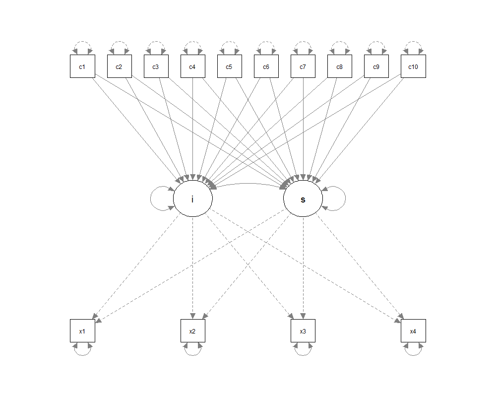
Figure 1: Growth curve model with 10 predictors of both the intercept and slope

Regularization

Although a host of methods exist to perform variable selection, the use of regularization has seen a wide array of application in the context of regression, and more recently, in areas such as graphical modeling, as well as a host of others. The two most common procedures for regularization in regression are the ridge [Hoerl and Kennard, 1970] and the least absolute shrinkage and selection operator [lasso; Tibshirani, 1996]; however, there are various alternative forms that can be seen as subsets or generalizations of these two procedures. Given an outcome vector y and predictor matrix $X\in{R}^{n\times p}$ , ridge estimates are defined as

$$\hat{\beta}^{ridge}=argmin\Big{\{}\sum_{i=1}^{N}(y_{i}=\beta_{0}-\sum_{j=1}^{p}x_{ij}\beta_{j})^{2}+\lambda\sum_{j=1}^{p}\beta_{j}^{2}\Big{\}},$$

where $\beta_{0}$ is the intercept, $\beta_{j}$ is the coefficient for $x_{j}$, and $\lambda$ is the penalty that controls the amount of shrinkage. Note that when $\lambda=0$, Equation 3 reduces to ordinary least squares regression. As $\lambda$ is increased, the $\beta$ parameters are shrunken towards zero. The lasso estimates are defined as

$$\hat{\beta}^{lasso}=argmin\Big{\{}\sum_{i=1}^{N}(y_{i}=\beta_{0}-\sum_{j=1}^{p}x_{ij}\beta_{j})^{2}+\lambda\sum_{j=1}^{p}|\beta_{j}|\Big{\}}.$$

In lasso regression, the $l_{1}$-norm is used, instead of $l_{2}$-norm as in ridge, which also shrinks the $\beta$ parameters, but additionally drives the parameters all the way to zero, thus performing a form of subset selection.

In the context of our example depicted in Figure 1, to use lasso regression to select among the covariates, the growth model would need to be reduced to two factor scores, which neglects both the relationship between both the slope and intercept, reducing both to independent variables. Particularly in models with a greater number of latent variables, this becomes increasingly problematic. A method that keeps the model structure, while allowing for penalized estimation of specific parameters is regularized structural equation modeling [RegSEM; Jacobucci et al., 2016]. RegSEM adds a penalty function to the traditional maximum likelihood estimation (MLE) for structural equation models (SEMs). The maximum likelihood cost function for SEMs can be written as

$$F_{ML}=log(\left|\Sigma\right|)+tr(C*\Sigma^{-1})-log(\left|C\right|)-p.$$

where $\Sigma$ is the model implied covariance matrix, $C$ is the observed covariance matrix, and $p$ is the number of estimated parameters. RegSEM builds in an additional element to penalize certain model parameters yielding

$$F_{regsem}=F_{ML}+\lambda P(\cdot)$$

where $\lambda$ is the regularization parameter and takes on a value between zero and infinity. When $\lambda$ is zero, MLE is performed, and when $\lambda$ is infinity, all penalized parameters are shrunk to zero. $P(\cdot)$ is a general function for summing the values of one or more of the model’s parameter matrices. Two common forms of $P(\cdot)$ include both the lasso ($\|\cdot\|_{1}$), which penalizes the sum of the absolute values of the parameters, and ridge ($\|\cdot\|_{2}$), which penalizes the sum of the squared values of the parameters.

In our example, the twenty regression parameters from the covariates to both the intercept and slope would be penalized. Using lasso penalties, the absolute value of these twenty parameters would be summed and after being multiplied by the penalty $\lambda$, added to equation 4, resulting in:

$$F_{lasso}=F_{ML}+\lambda*\left\|\begin{matrix}c1_{i}\\ c2_{i}\\ \vdots\\ c10_{i}\\ c1_{s}\\ \vdots\\ c10_{s}\\ \end{matrix}\right\|_{1}$$

Although the fit of the model is easily calculated given a set of parameter estimates, traditional optimization procedures for SEM cannot be used given the non-differentiable nature of lasso penalties, and as detailed later, sparse extensions.

Optimization

One method that has become popular for optimizing penalized likelihood method is that of proximal gradient descent [e.g. p. 104 in Hastie et al., 2015]. In comparison to one-step procedures common in SEM optimization, that only involve a method for calculating the step size and the direction (typically using the gradient and an approximation of the Hessian), proximal gradient descent can be formulated as a two-step procedure. With a stepsize of $s^{t}$ and parameters $\theta^{t}$ at iteration t:

1. First, take a gradient step size $z=\theta^{t}-s^{t}\nabla g(\theta^{t})$.

2. Second, perform elementwise soft-thresholding $\theta^{t+1}=S_{s^{t}\lambda}(z)$.

where $S_{s^{t}\lambda}(z)$ is the soft-thresholding operator [Donoho, 1995] used to overcome non-differentiability of the lasso penalty at the origin:

$$S_{s^{t}\lambda}(z_{j})=sign(\theta_{j})(|\theta_{j}|-s^{t}\lambda)_{+}.$$ (1)

In this, $(x)_{+}$ is shorthand for max(x,0) and $s^{t}$ is the step size. Henceforth, $\lambda$ is assumed to encompass both the penalty and the step size $s^{t}$. This procedure is only used to update parameters that are subject to penalty. Non-penalized parameters are updated only using step 1 from above.

However, in testing with larger SEMs, the use of only the gradient for minimization has been found to cause problems. Particularly at higher penalties, estimation of both observed and latent variances can become difficult, as these parameter estimates can become inflated if the optimization routine has a hard time finding an optima. Due to this, for larger models it is recommended to use a quasi-Newton method, specifically the BFGS (Broyden-Fletcher-Goldfarb-Shanno) algorithm. This method involves computing approximations to the Hessian matrix of the objective function, in which step 1 above is replaced with:

$$z=\theta^{t}-s^{t}H^{-1}\nabla g(\theta^{t}).$$ (2)

Although calculating the approximation to the Hessian is computationally intensive, this minimization method paired with a backtracking rule for finding the step size ($s^{t}$) has been found to be only slightly slower than gradient descent. However, more testing is needed to determine more specifically which settings each of the optimization methods may be preferential.

Types of Penalties

Outside of both ridge and lasso penalties, a host of additional forms of regularization exist.

Elastic Net

Most notably, the elastic net [Zou and Hastie, 2005] encompasses both the ridge and lasso, reaching a compromise between both through the addition of an additional parameter $\alpha$, manifesting itself as

$$P_{enet}(\theta_{j})=(1-\alpha)\|\theta_{j}\|_{2}+\alpha\|\theta_{j}\|_{1}$$

with a soft-thresholding update of

$$S(\theta_{j})=\begin{cases}0,&|\theta_{j}|<\alpha\lambda\\ \frac{sgn(\theta_{j})(|\theta_{j}|-\alpha\lambda)}{1+(1-\alpha)\lambda},&|\theta_{j}|\geq\alpha\lambda\end{cases}$$

When $\alpha$ is zero, ridge is performed, and conversely when $\alpha$ is 1, lasso regularization is performed. This method harnesses the benefits of both methods, particularly when variable selection is warranted (lasso), but there may be collinearity between the variables (ridge).

Adaptive Lasso

In using lasso penalties, difficulties emerge when the scale of variables differ dramatically. By only using one value of $\lambda$, this can add appreciable bias to the resulting estimates [e.g. Fan and Li, 2001]. One method proposed for overcoming this limitation is the adaptive lasso [Zou, 2006]. Instead of penalizing parameters directly, each parameter is scaled by the un-penalized estimated (MLE parameter estimates in SEM). The adaptive lasso results in:

$$F_{alasso}=F_{ML}+\lambda\|\theta_{ML}^{-1}*\theta_{pen}\|_{1}$$

with, following the same form for the lasso, the soft-thresholding update is:

$$S(\theta_{j})=sign(\theta_{j})(|\theta_{j}|-\frac{\lambda}{2|\theta_{j}|})_{+}$$

In this, larger penalties are given for non-significant (smaller) parameters, limiting the bias in estimating larger, significant parameters. Note that one limitation of this approach for SEM models is that the model needs to be estimable with MLE. Particularly for models with large numbers of variables, in relation to sample size, this may not be possible.

Sparse Extensions

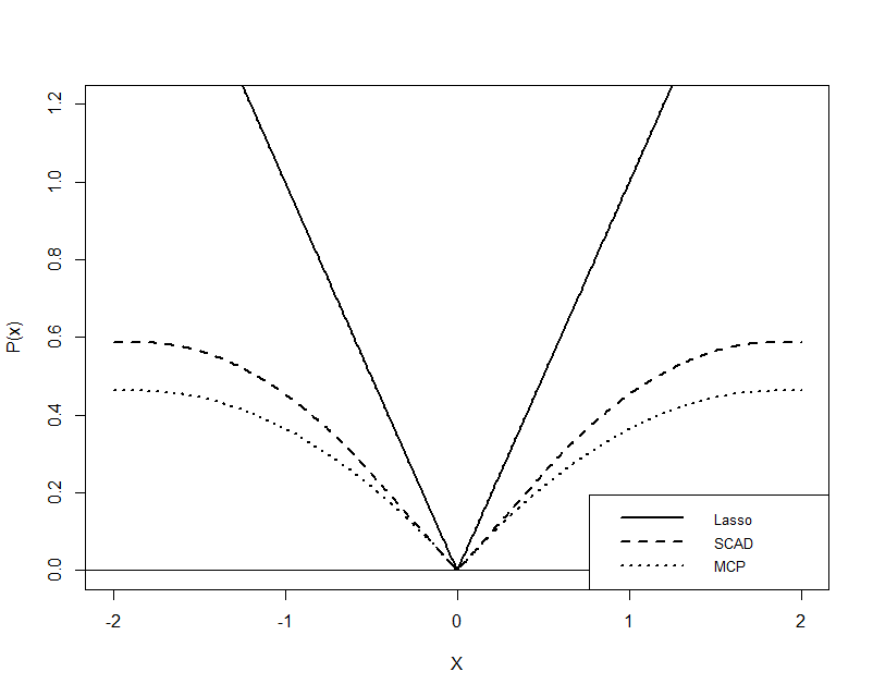
Figure 2: Comparison of types of penalties with $\lambda=0.5$

Two additional penalties that overcome some of the deficiencies of the lasso, producing sparser solutions, include the smoothly clipped absolute deviation penalty [SCAD; Fan and Li, 2001] and the minimax concave penalty [MCP; Zhang, 2010]. In comparison to the lasso, both the SCAD and MCP have much smaller penalties for large parameters, where the amount of penalty for small penalties is similar to the lasso, as is evident in Figure 2.

The SCAD takes the form of:

$$pen_{\lambda,\gamma}(\theta_{j})=\lambda\big{\{}I(\theta_{j}\leq\lambda)+\frac{(\gamma\lambda-0)_{+}}{(\gamma-1)\lambda}I(\theta_{j}>\lambda)\big{\}}$$

with a soft-thresholding update of

$$S(\theta_{j})=\begin{cases}S(\theta_{j},\lambda),&|\theta_{j}|\geq 2\lambda\\ \frac{\gamma-1}{\gamma-2}S(\theta_{j},\frac{\lambda\gamma}{\gamma-1}),&2\lambda<|\theta_{j}|\leq\alpha\lambda\\ \theta_{j}&|\theta_{j}|>\lambda\gamma\end{cases}$$

for $\gamma>2$. As the the penalty in equation 11 is non-convex (as is the MCP), this makes the computation more difficult. However, in the context of SEM this can be seen as less problematic, as equation 3 is also non-convex.

Additionally, the MCP takes the form of:

$$pen_{\lambda,\gamma}(\theta_{j})=\lambda\bigg{(}|\theta_{j}|-\frac{\theta_{j}^{2}}{2\lambda\gamma}\bigg{)}I(|\theta_{j}|<\lambda\gamma)+\frac{\lambda^{2}\gamma}{2}I(|\theta_{j}|\geq\lambda\gamma)$$

with a soft-thresholding update of

$$S(\theta_{j})=\begin{cases}\frac{\gamma}{\gamma-1}S(\theta_{j},\lambda),&|\theta_{j}|\leq\lambda\gamma\\ \theta_{j}&|\theta_{j}|>\lambda\gamma\end{cases}$$

for $\gamma>0$. As seen in Figure 2, this results in similar amount of shrinkage for smaller estimates in comparison to the SCAD, however, less for larger estimates. For both the SCAD and MCP, both the $\gamma$ and $\lambda$ parameters are used as hyper-parameters. This involves testing models over a two-dimensional array of parameters, however, in regsem, $\gamma$ is by default fixed to 3.7 per Fan and Li [2001].

Implementation

RegSEM is implemented as the regsem package [Jacobucci, 2017] in the R statistical environment [R Core Team, 2017]. To estimate the maximum likelihood fit of the model, regsem uses Reticular Action Model [RAM; McArdle and McDonald, 1984, McArdle, 2005] notation to derive an implied covariance matrix. The parameters of each SEM are translated into three matrices: the filter (F), the asymmetric (A; directed paths; e.g. factor loadings or regressions), and the symmetric (S; undirected paths; e.g. covariances or variances). See Jacobucci et al. [2016] for more detail on RAM notation and its application to RegSEM.

Syntax for using the regsem package is based on the lavaan package [Rosseel, 2012] for structural equation models. lavaan is a general SEM software program that can fit a wide array of models with various estimation methods. To use regsem, the user has to first fit the model in lavaan. Note that particularly in cases that the number of variables is larger than the sample size, the model in lavaan does not need to converge, let alone run. In this case, the do.fit=FALSE argument in lavaan can be used. Additionally, regsem only works with models that assume the variables are continuous, thus none of the additional options in lavaan that accomodate categorical variables (e.g. the WLSMV estimator with ordered indicators) are available.

As a canonical example, below is the code for a confirmatory factor analysis model with one latent factor and seven indicators from the bfi dataset from the psych package [Revelle, 2014].

library(psych);library(lavaan)

bfi2 <- bfi[1:250,c(1:5,18,22)]

bfi2[,1] <- reverse.code(-1,bfi2[,1])

mod <- "

f1 =~ NA*A1+A2+A3+A4+A5+O2+N3

f1~~1*f1

"

out <- cfa(mod,bfi2)

#summary(out)

After a model is run in lavaan, using lavaan() or any of the wrapper functions for fitting a model (i.e. sem(), cfa(), or growth()), the object is then used by the regsem package to translate the model into RAM notation and run using one of three functions: regsem(), multi_optim(), or cv_regsem(). The regsem() function runs a model with one penalty value, whereas multi_optim() does the same but allows for the use of random starting values. However, the main function is cv_regsem(), as this not only runs the model, but runs it across a vector of varying penalty values. textbf{cv_regsem()} was originally created to solely use k-fold cross-validation to test penalties and choose a final model (hence the name). However, as it currently stands, it is recommended to run the model using the entire sample, paired with the use of an information criteria to choose a final model. The use of bootstrapping or k-fold cross-validation requires additional research and is discussed further in the Discussion.

In the above one-factor model, each of the factor loadings can be tested with lasso penalties to determine whether each indicator is a necessary component of the latent factor. The first step is to identify which parameters are to be penalized, and pass this information to regsem. The easiest way to accomplish this is through the use of extractMatrices():

library(regsem)

extractMatrices(out)$A

##    A1 A2 A3 A4 A5 O2 N3 f1
## A1  0  0  0  0  0  0  0  1
## A2  0  0  0  0  0  0  0  2
## A3  0  0  0  0  0  0  0  3
## A4  0  0  0  0  0  0  0  4
## A5  0  0  0  0  0  0  0  5
## O2  0  0  0  0  0  0  0  6
## N3  0  0  0  0  0  0  0  7
## f1  0  0  0  0  0  0  0  0

In this, extractMatrices() allows the user to examine how the lavaan model is translated into RAM matrices. Further, by looking at the A matrix (directed paths which originate at the column name and go to the row name), one can identify the parameter numbers corresponding to the factor loadings of interest for regularization. For this model, the factor loadings represent parameter numbers one through seven, of which we pass directly to the pars_pen argument of the cv_regsem() function (if pars_pen=NULL then all directed effects, outside of intercepts, are penalized). Additionally, if parameter labels are used in the lavaan model specification, these can be directly passed to regsem in the pars_pen argument.

Additionally, we pass the arguments of how many values of penalty we want to test (n.lambda=15), how much the penalty should increase for each model (jump=.05), and finally that lasso estimation is used (type="lasso").

out.reg <- cv_regsem(out, type="lasso",

                     pars_pen=c(1:7),n.lambda=23,jump=.05)

The out.reg object contains two components, out.reg$fits has the parameter estimates for each of the 15 models,

head(round(out.reg$parameters,2),5)

##      f1 -> A1 f1 -> A2 f1 -> A3 f1 -> A4 f1 -> A5 f1 -> O2 f1 -> N3
## [1,]     0.56     0.77     1.08     0.70     0.90    -0.03    -0.08
## [2,]     0.53     0.74     1.05     0.66     0.87     0.00    -0.05
## [3,]     0.50     0.72     1.03     0.62     0.84     0.00    -0.01
## [4,]     0.47     0.69     1.01     0.58     0.81     0.00     0.00
## [5,]     0.44     0.67     0.99     0.55     0.79     0.00     0.00
##      A1 ~~ A1 A2 ~~ A2 A3 ~~ A3 A4 ~~ A4 A5 ~~ A5 O2 ~~ O2 N3 ~~ N3
## [1,]     1.52     0.69     0.53     1.84     0.88     2.45     2.29
## [2,]     1.53     0.70     0.52     1.84     0.89     2.45     2.29
## [3,]     1.53     0.70     0.52     1.85     0.90     2.45     2.30
## [4,]     1.54     0.71     0.52     1.86     0.90     2.45     2.30
## [5,]     1.55     0.71     0.51     1.87     0.91     2.45     2.30

while out.reg$fits contains information pertaining to the fit of each model:

head(round(out.reg$fits,2))

##      lambda conv rmsea     BIC
## [1,]   0.00    0  0.08 5713.57
## [2,]   0.05    0  0.08 5708.76
## [3,]   0.10    0  0.08 5710.45
## [4,]   0.15    0  0.08 5707.20
## [5,]   0.20    0  0.09 5709.89
## [6,]   0.25    0  0.09 5713.11

In this, the user can examine the penalty (lambda), whether the model converged (“conv”=0 means converged, whereas either 1 or 99 is non-convergence), and the fit of each model. By default, two fit indices are output, both the root mean square error of approximation [RMSEA; Steiger and Lind, 1980], and the Bayesian information criteria [BIC; Schwarz, 1978]. Both the RMSEA and BIC take into account the degrees of freedom of the model, an important point for model selection in the presence of lasso penalties (and other penalties that set parameters to zero). Zou et al. [2007] proved that the number of nonzero coefficients is an unbiased estimate of the degrees of freedom for regression. As the penalty increases, select parameters are set to zero, thus increasing the degrees of freedom, which for fit indices that include the degrees of freedom in the calculation, means that although $F_{ML}$ may only get worse (increase), both the RMSEA and BIC can improve (decrease).

Instead of examining the out.reg$fits output matrix of parameter estimates, users also have the option to plot the trajectory of each of the penalized parameters. This is accomplished with

plot(out.reg,show.minimum="BIC")

After a final model (penalty) is chosen, users have the option either just use the output from cv_regsem(), or the final model can be re-run with either regsem() or multi_optim() to attain additional information. In the model above, the best fitting penalty, according to the BIC, is $\lambda=0.15$.

summary(out.reg)

## CV regsem Object
##  Number of parameters regularized: 7
##  Lambda ranging from 0 to 1.1
##  Lowest Fit Lambda: 0.15
##  Metric: BIC
##  Number Converged: 23

Instead of having to re-run the model with regsem() to get the final parameter estimates, a user can specify what fit index should be used to choose a final model with metric = in cv_regsem(). These estimates are printed in:

out.reg$final_pars

## f1 -> A1 f1 -> A2 f1 -> A3 f1 -> A4 f1 -> A5 f1 -> O2 f1 -> N3 A1 ~~ A1
##    0.467    0.692    1.006    0.584    0.811    0.000    0.000    1.540
## A2 ~~ A2 A3 ~~ A3 A4 ~~ A4 A5 ~~ A5 O2 ~~ O2 N3 ~~ N3
##    0.707    0.515    1.859    0.903    2.448    2.298

Additional fit indices can be attained through the fit_indices() function if only one model was run with either regsem() or multi_optim(). These same fit measures can be accessed through cv_regsem() through changing the defaults with the fit.ret=c("rmsea","BIC") argument. Finally, instead of assessing these fit indices on the same sample that the models were run on, a holdout dataset could be used. This can be done two ways: either with cv_regsem(…,fit.ret2="test") or with fit_indices(model,CV=TRUE,CovMat=) and specifying the name of the holdout covariance matrix.

Structural equation modeling is hard, and pairing with regularization doesn’t make it any easier. Given this, and the number of options available in the regsem package, a Google group forum was created in order to answer questions and trouble shoot at https://groups.google.com/forum/#!forum/regsem.

Comparison

To compare the different types of penalties in regsem, we return to the the initial example of the latent growth curve model displayed in Figure 1. Using the same simulated data, the model can be run in lavaan as

mod1 <- "

i =~ 1*x1 + 1*x2 + 1*x3 + 1*x4

s =~ 0*x1 + 1*x2 + 2*x3 + 3*x4

i ~ c1 + c2 + c3 + c4 + c5 + c6 + c7 + c8 + c9 + c10

s ~ c1 + c2 + c3 + c4 + c5 + c6 + c7 + c8 + c9 + c10

"

lav.growth <- growth(mod1,dat,fixed.x=T)

Comparing different types of penalties in regsem requires a different specification of the type argument. The options currently include maximum likelihood ("none"), ridge ("ridge"), lasso ("lasso"; the default), adaptive lasso ("alasso"), elastic net ("enet"), SCAD ("scad"), and MCP ("mcp"). For the elastic net, there is an additional hyperparameter, alpha that controls the tradeoff between ridge and lasso penalties. This is specified as alpha= , which has a default of 0.5. Additionally, both the SCAD and MCP have the additional hyper parameter of gamma, which is specified as gamma= and defaults to 3.7 per Fan and Li [2001].

For the purposes of comparison, each of the 20 covariate regressions were penalized using the lasso, adaptive lasso, SCAD, and MCP, and compared to the maximum likelihood estimates. In this model, the data were simulated to have two large effects (both c1 parameters), two small effects (both c2 parameters) and sixteen true zero effects (c3-c10 parameters). Note that the covariates were simulated to have zero covariance among each variable. If there was substantial collinearity among covariates, the elastic net would be more appropriate to simultaneously select predictors while also accounting for the collinearity. The parameter estimates corresponding the the best fit of the BIC are has the fit of each model, resulting in Table 1, created using the xtable package [Dahl, 2009].

	MLE	lasso	alasso	SCAD	MCP
$c1_{i}$	0.92*	0.72	0.91	0.94	0.92
$c2_{i}$	0.07	0.00	0.00	0.00	0.00
$c3_{i}$	0.10	0.00	0.00	0.00	0.00
$c4_{i}$	0.07	0.00	0.00	0.00	0.00
$c5_{i}$	0.04	0.00	0.00	0.00	0.00
$c6_{i}$	-0.25	0.00	0.00	0.00	-0.19
$c7_{i}$	0.11	0.00	0.00	0.00	0.00
$c8_{i}$	-0.13	0.00	0.00	0.00	0.00
$c9_{i}$	-0.03	0.00	0.00	0.00	0.00
$c10_{i}$	0.09	0.00	0.00	0.00	0.00
$c1_{s}$	1.18*	1.09	1.22	1.24	1.24
$c2_{s}$	0.29*	0.19	0.28	0.35	0.35
$c3_{s}$	0.18	0.09	0.00	0.00	0.00
$c4_{s}$	-0.08	0.00	0.00	0.00	0.00
$c5_{s}$	-0.18	0.00	0.00	0.00	0.00
$c6_{s}$	0.25*	0.00	0.00	0.00	0.00
$c7_{s}$	-0.18	-0.04	0.00	0.00	0.00
$c8_{s}$	0.26*	0.10	0.00	0.00	0.00
$c9_{s}$	-0.06	0.00	0.00	0.00	0.00
$c10_{s}$	0.08	0.00	0.00	0.00	0.00
BIC	3465.28	3427.46	3415.05	3414.38	3417.20

Table 1: Parameter estimates for the final models across five estimation methods. Note that * represent significant parameters at p < .05 for maximum likelihood estimation.

While every regularization method erroneously set both simulated true intercept effects as zero (non-significant in MLE), both the adaptive lasso and SCAD correctly identified every true zero effect. The lasso identified two false effects while the MCP mistakenly identified one. Additionally, the lasso estimation of the true effects was attentuated in comparison to the other regularization methods. This is in line with previous research [Fan and Li, 2001], necessitating the use of a two-step relaxed lasso method Meinshausen, 2007; Jacobucci et al., 2016, see As expected given the small ratio between number of estimated parameters and sample size, MLE mistakenly identified 3 false effects as significant.

To compare the performance of each penalization method further, particularly in the presence of a small parameter to sample size ratio, a small simulation study was conducted. The same model and effects was kept, but the sample size was varied to include 80, 200, and 1000 to demonstrate how MLE improves as sample size increases, while each of the regularization methods performs well regardless of sample size. Each run was replicated 200 times. For each regularization method, the BIC was used to choose a final model among the 40 penalty vales. The results are displayed in Table 2.

	N	ML	lasso	alasso	SCAD	MCP
	80.00	0.08	0.08	0.04	0.05	0.20
False Positives	200.00	0.06	0.05	0.02	0.03	0.06
	1000.00	0.05	0.08	0.01	0.01	0.02
	80.00	0.33	0.31	0.35	0.35	0.31
False Negatives	200.00	0.19	0.19	0.23	0.26	0.27
	1000.00	0.00	0.00	0.00	0.01	0.03

Table 2: Results from the simulation using the model in Figure 1. Each condition was replicated 200 times. False positives represent concluding that the simulated regressions of zero were concluded as nonzero. False negatives are concluding that either the simulated regression values of 1 or 0.2 are in fact zero. Bolded values represent the smallest error per condition.

For false positives, the adaptive lasso demonstrated the best performance, where the performance of MLE leveled off at the 0.05 level at a sample size of 1000 as expected. For false negatives, lasso penalties demonstrated similar results to MLE. This was expected given the tendency of the lasso to under-penalize small coefficients in comparison to the other regularization methods. The adaptive lasso and SCAD demonstrated slightly worse results, however, outside of the MCP, each method made either zero or near zero errors at a sample size of 1000. The poor performance of the MCP may be in part due to fixing the $\gamma$ penalty to 3.7. Varying this parameter may improve the performance of the method. In summary, the regularization methods demonstrated an improvement over maximum likelihood, particularly at small samples, for a model that had a large number of estimated parameters.

Discussion

This paper provides an introduction to the regsem package, outlining the mathematical details of regularized structural equation modeling [RegSEM; Jacobucci et al., 2016] and the usage of the regsem package. RegSEM allows the use of regularization while keeping the structural equation model intact, adding penalization directly into the estimation of the model. The application of RegSEM was detailed using two example models: a latent growth curve model with 20 predictors of both the latent intercept and slope, along with a factor analysis with one latent factor. With the latent growth curve model, the small parameter to sample size ratio resulted in a larger number of false positives in using maximum likelihood estimation. In both the simulated example and the small simulation, the different types of regularization in regsem demonstrated better false positive and negative rates in comparison to maxiumum likelihood across sample sizes.

Broadly speaking, there is a growing amount of research into the integration between data mining methods and latent variable models. Specifically, beyond RegSEM, this has taken the form of item response theory and regularization [Sun et al., 2016], other regularization and latent variable formulations [Hirose and Yamamoto, 2013, Huang et al., 2017], pairing both structural equation models with decision trees [Brandmaier et al., 2013], exploratory psychological network analaysis [e.g. Epskamp et al., 2016], along with many others. The amount of pairing between methods that have generally been housed in separate camps will only increase into the future. This type of research will be facilitated by the general upsurge in the creation of open source software that gives users a general framework to test models. This was the motivation behind creating the regsem package, in that users can estimate models ranging from simple factor analysis models, to latent longitudinal models with few to many time points, and finally to models with a large number of latent and observed variables. The use of regularization allows for the estimation of much larger structural equation models than before. However, sample sizes in the social and behavioral sciences are typically not large. To estimate large models with small sample sizes invites increasing amounts of bias as demonstrated with the simulated data in this paper. Regularization can be used to reduce the complexity of the model, thus decreasing both the bias and variance.

With highly constrained structural equation models, achieving model convergence can be particularly problematic in using regsem. For instance, with the latent change score model [McArdle and Hamagami, 2001], Bayesian regularization methods have less difficulty in reaching convergence across chains [Jacobucci and Grimm, 2017]. With the recent advent of additional sparsity inducing priors, along with new forms of software such as Stan [Carpenter et al., 2016], for some models it may be more appropriate to use these Bayesian regularization methods over their frequentist counterparts. In the realm of Bayesian regularization for structural equation models, although some research exists [Feng et al., 2017], much more is warranted.

Future research with regsem should focus on a number of avenues. One is comparing the different forms of regularization, delineating which method may be best in which setting. Additionally, as structural equation models become larger, with the advent of much larger datasets, computational speed will become a principal concern. Although 40 penalties in the models tested above can be run in a matter of seconds on a standard laptop, larger models can take much longer. To handle this, future implementation with regsem will test the inclusion of different types of optimization, specifically testing whether coordinate descent algorithms [Friedman et al., 2010] can speed up convergence. Finally, although the use of bootstrapping or k-fold cross-validation is computationally intensive, these forms of resampling (paired with a fit index that does not have a penalty for the number of parameters, i.e. $\chi^{2}$) may produce better results for both ridge and elastic net penalties, where it is less clear how to take into account parameter shrinkage for choosing a final model.

Conclusion

This paper provided a brief overview on the use of the regsem package as an implementation of regularized structural equation modeling. Because structural equation modeling encompasses a wide array of latent variable models, the regsem package was created as a general package for including different forms of regularization into a host of latent variable models. RegSEM, and thus the regsem package, has been evaluated in a wide array of SEM models, including confirmatory factor analysis [Jacobucci et al., 2016], latent change score models [Jacobucci and Grimm, 2017], and mediation models [Serang et al., in press]. Future updates to regsem will focus on decreasing the computational time of large latent variable models in order to provide an avenue of testing for researchers collecting larger and larger datasets. RegSEM is a method that operates at all ends of the data size spectrum: allowing for a reduction in complexity when the sample size is small, along with dimension reduction in the presence of large data (both $N$ and $P$).

References

- Brandmaier et al. [2013] Andreas M. Brandmaier, Timo von Oertzen, John J. McArdle, and Ulman Lindenberger. Structural equation model trees. Psychological Methods, 18(1):71–86, 2013.
- Carpenter et al. [2016] Bob Carpenter, Andrew Gelman, Matt Hoffman, Daniel Lee, Ben Goodrich, Michael Betancourt, Michael A Brubaker, Jiqiang Guo, Peter Li, and Allen Riddell. Stan: A probabilistic programming language. Journal of Statistical Software, 20, 2016.
- Dahl [2009] David B Dahl. xtable: Export tables to latex or html. R package version, pages 1–5, 2009.
- Donoho [1995] David L Donoho. De-noising by soft-thresholding. IEEE transactions on information theory, 41(3):613–627, 1995.
- Epskamp et al. [2016] Sacha Epskamp, Mijke Rhemtulla, and Denny Borsboom. Generalized network psychometrics: Combining network and latent variable models. Psychometrika, pages 1–24, 2016.
- Fan and Li [2001] Jianqing Fan and Runze Li. Variable selection via nonconcave penalized likelihood and its oracle properties. Journal of the American statistical Association, 96(456):1348–1360, 2001.
- Feng et al. [2017] Xiang-Nan Feng, Hao-Tian Wu, and Xin-Yuan Song. Bayesian regularized multivariate generalized latent variable models. Structural Equation Modeling: A Multidisciplinary Journal, pages 1–18, 2017.
- Friedman et al. [2010] Jerome Friedman, Trevor Hastie, and Rob Tibshirani. Regularization paths for generalized linear models via coordinate descent. Journal of statistical software, 33(1):1, 2010.
- Hastie et al. [2015] Trevor Hastie, Robert Tibshirani, and Martin Wainwright. Statistical Learning with Sparsity: The Lasso and Generalizations. CRC Press, 2015.
- Hirose and Yamamoto [2013] Kei Hirose and Michio Yamamoto. fanc: Penalized Likelihood Factor Analysis via Nonconvex Penalty, 2013. URL http://CRAN.R-project.org/package=fanc. R package version 1.13.
- Hoerl and Kennard [1970] Arthur E Hoerl and Robert W Kennard. Ridge regression: Biased estimation for nonorthogonal problems. Technometrics, 12(1):55–67, 1970.
- Huang et al. [2017] Po-Hsien Huang, Hung Chen, and Li-Jen Weng. A penalized likelihood method for structural equation modeling. Psychometrika, pages 1–26, 2017.
- Jacobucci [2017] Ross Jacobucci. Package ’regsem’, 2017.
- Jacobucci and Grimm [2017] Ross Jacobucci and K. J. Grimm. Regularized estimation of multivariate latent change score models. Advances in Longitudinal Models for Multivariate Psychology: A Festschrift for Jack McArdle, 2017.
- Jacobucci et al. [2016] Ross Jacobucci, Kevin J Grimm, and John J McArdle. Regularized structural equation modeling. Structural Equation Modeling: A Multidisciplinary Journal, 23(4):555–566, 2016.
- Kline [2015] Rex B Kline. Principles and practice of structural equation modeling. Guilford publications, 2015.
- McArdle [2005] John J McArdle. The development of the ram rules for latent variable structural equation modeling. Contemporary psychometrics: A festschrift for Roderick P. McDonald, pages 225–273, 2005.
- McArdle and Hamagami [2001] John J McArdle and Fumiaki Hamagami. Latent difference score structural models for linear dynamic analyses with incomplete longitudinal data. 2001.
- McArdle and McDonald [1984] John J McArdle and Roderick P. McDonald. Some algebraic properties of the reticular action model for moment structures. British Journal of Mathematical and Statistical Psychology, 37(2):234–251, 1984.
- Meinshausen [2007] Nicolai Meinshausen. Relaxed lasso. Computational Statistics & Data Analysis, 52(1):374–393, 2007.
- Meredith and Tisak [1990] William Meredith and John Tisak. Latent curve analysis. Psychometrika, 55(1):107–122, 1990.
- R Core Team [2017] R Core Team. R: A Language and Environment for Statistical Computing. R Foundation for Statistical Computing, Vienna, Austria, 2017.
- Revelle [2014] William Revelle. psych: Procedures for psychological, psychometric, and personality research. Northwestern University, Evanston, Illinois, 165, 2014.
- Rosseel [2012] Yves Rosseel. lavaan: An r package for structural equation modeling. Journal of Statistical Software, 48(2):1–36, 2012.
- Schwarz [1978] Gideon Schwarz. Estimating the dimension of a model. The annals of statistics, 6(2):461–464, 1978.
- Serang et al. [in press] Sarfaraz Serang, Ross Jacobucci, Kim Brimhall, and Kevin J Grimm. Exploratory mediation analysis via regularization. Structural Equation Modeling: A Multidisciplinary Journal, in press.
- Steiger and Lind [1980] James H Steiger and John C Lind. Statistically based tests for the number of common factors. In annual meeting of the Psychometric Society, Iowa City, IA, volume 758, 1980.
- Sun et al. [2016] Jianan Sun, Yunxiao Chen, Jingchen Liu, Zhiliang Ying, and Tao Xin. Latent variable selection for multidimensional item response theory models via l_ 1 regularization. Psychometrika, 81(4):921–939, 2016.
- Tibshirani [1996] Robert Tibshirani. Regression shrinkage and selection via the lasso. Journal of the Royal Statistical Society. Series B (Methodological), 58(1):267–288, 1996. ISSN 00359246.
- Zhang [2010] Cun-Hui Zhang. Nearly unbiased variable selection under minimax concave penalty. The Annals of statistics, 38(2):894–942, 2010.
- Zou [2006] Hui Zou. The adaptive lasso and its oracle properties. Journal of the American statistical association, 101(476):1418–1429, 2006.
- Zou and Hastie [2005] Hui Zou and Trevor Hastie. Regularization and variable selection via the elastic net. Journal of the Royal Statistical Society: Series B (Statistical Methodology), 67(2):301–320, 2005.
- Zou et al. [2007] Hui Zou, Trevor Hastie, and Robert Tibshirani. On the “degrees of freedom” of the lasso. The Annals of Statistics, 35(5):2173–2192, 2007. doi: 10.1214/009053607000000127.