Long-Term Evolution of Genetic Programming Populations

Abstract

We evolve binary mux-6 trees for up to 100 000 generations evolving some programs with more than a hundred million nodes. Our unbounded Long-Term Evolution Experiment LTEE GP appears not to evolve building blocks but does suggests a limit to bloat. We do see periods of tens even hundreds of generations where the population is 100% functionally converged. The distribution of tree sizes is not as predicted by theory.

Short version appears as [21].

Keywords GP, Convergence, Long-Term Evolution Experiment LTEE Extended unbounded evolution

1 Introduction

Rich Lenski’s experiments in long term evolution [1] in which the BEACON team evolved bacteria for more than 60 000 generations and found continued beneficial adaptive mutations, prompts the same question in computation based evolution. What happens if we allow artificial evolution, specifically genetic programming (GP) with crossover [2, 3, 4], to evolve for tens of thousands, even a hundred thousand generations.

Firstly we expect bloat, and so we need a GP system not only able to run for $10^{5}$ generations but also able to process trees with in excess of a 100 million nodes. Section 2 describes our target system which is able to do this on a Linux desktop computer. Section 2.1 shows we do indeed see bloat but after a few hundred generations we start to see surprises. Tree growth is not continuous. Indeed we see many generations where the trees get smaller. As we look at the very long term distribution of fitness in Section 2.2 we do not get the whole population reaching one fitness value and everyone having that fitness in all subsequent generations. Section 2.2 also applies existing theory to give a mathematical model of fitness convergence’s impact on selection.

Section 2.3 discusses introns and constants. By introns we mean subtrees which cannot impact on the program’s output, even if modified by crossover. A constant is simply a subtree whose output is the same for all input test cases. Although introns are well known in GP, we find constants are also required to explain the observed long term evolution. In Section 2.4 we confirm the asymmetry of the GP crossover and the importance of the first parent, which gives the offspring’s root node and show this becomes even more important in long term evolution. (Since this parent typically gives more genetic material we call it the mother, or simply mum.) Section 2.5 looks at the distribution of values within the large evolved trees and particularly how combining values within the evolving trees leads to constants.

Section 2.6 considers the evolution of multiple solutions as an alternative to classic bloat as protection from disruptive crossover. However it concludes that although multiple solutions within the highly evolved programs are possible, they do not explain the evolution seen. Whereas Section 2.7 shows the fraction of constants in highly evolved trees is fairly stable despite huge fluctuations in the size of the trees containing them.

Section 2.8 shows the classic fractal Flajolet random distribution of trees [8] still applies to highly evolved trees. It also shows, as expected, the Flajolet distribution also applies to the sub trees within them. Finally Section 2.9 demonstrates the common assumption that useful code clusters around the root node and shows that in the longer term this code becomes highly stable and is surrounded and is protected by many thousands of useless instructions composed of both introns and constants.

Section 3 proposes a lose limit to bloat in extremely long GP runs. The limit turns out to be somewhat ragged. Nevertheless Section 3 provides some experimental evidence for it in runs lasting one hundred thousand generations.

1.1 Background

There has been some work in evolutionary computing and artificial life looking at the extended evolutionary process itself rather than focusing on solving a problem. For example, Harvey’s Species Adaptation Genetic Algorithms (SAGA) [9] argued in favour of variable length representation (such as we use in genetic programming) to allow continued evolutionary adaptation. Whilst more recently Lewis’ TMBL system [10] turned to the power of parallel processing GPUs to investigate the long term gathering of small mutations over many generations.

McPhee [11, sect. 1.2] reported that his earlier studies which had reported the first 100 generations of the INC-IGNORE problem could not safely be extrapolated to long term evolution but considered runs of up to 3000 generations. McPhee [11] found “increasing amount of noise” in the evolution of their linear unary trees and say it was unclear if their tree lengths would be bounded. As in our previous work [12] we will use binary tree GP. However previously [12] we only considered the first few hundred generations, whilst in the next sections we shall investigate many tens of thousands.

2 Results

Following [12], the generational GP was run with a population of 500 (see Table 1). All parents were selected using independent tournaments of size seven to select both parents used by each crossover. One child was created by each crossover. For simplicity, all crossover points are chosen uniformly at random. I.e. there was no bias in favour of functions [2]. Mutation was not used. Since we will evolve trees with more than a hundred million nodes it is essential to use a compact representation and fast fitness evaluation, therefore we use Poli’s Sub-machine code GP [13] on a 64 bit processor which allows us to process all 64 fitness cases simultaneously.

Table 1: Long term evolution of 6-Mux trees

Terminal set:	D0 D1 D2 D3 D4 D5
Function set:	AND OR NAND NOR
Fitness cases:	All $2^{6}$ combinations of inputs D0..D5
Selection:	tournament size 7 using the number of correct fitness cases
Population:	500. Panmictic, non-elitist, generational.
Parameters:	Initial population created at random using ramped half and half [2] with depth between 2 and 6. 100% subtree crossover [2]. 10 000 generations (runs cut short on any tree reaching hard limit of a million nodes).

2.1 Evolution of Size

In all cases we do see enormous increases in size (see Figure 1). Except for runs in Section 3, in each case the run was cut short because bloat became so severe that further crossovers where inhibited by the hard size limit of a million nodes (see Table 1). In the initial generations, we do see explosive growth in tree size and this continues even after a tree with max fitness is found. Indeed bloat continues even as the first time everyone in the population has the same fitness value ($1^{\rm st}$ convergence).

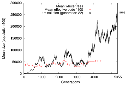
Figure 1: Evolution of tree size in first 6-mux run. (This run aborted after 5355 gens by first crossover to hit million node limit.) Because of computational cost, the average number of effective instructions (i.e. not introns or blocked by constants) is plotted ($+$) every 100 gens. (Mean effective code 497.)

If everyone in the population has the same fitness, selection appears to become random and children are as likely to be smaller than their parents as they are likely to be bigger. If selection is switched off for many generations, we do indeed see an apparently random walk in average tree size, with falls and rises. However tree size cannot go negative and once the population contains only small trees crossover cannot escape and the trees remain tiny forever. That is, we have a gambler’s ruin. (We return to this in Section 3.)

Although after the time where almost everyone in the population has the same fitness value, we do see falls in average tree size as well as increases, this is not a simple random walk. For example, in Figure 1 there are substantial falls in size which take place over many generations during which the number of generations in which the trees are smaller on average v. the number in which they are bigger, is too large to be simply random. This might be due to the discovery of smaller than average individuals of max fitness but with a higher than average effective fitness, however we were unable to find hard evidence to support this hypothesis. (Effective fitness is simply fitness rescaled to take into account the disruptive effects of crossover and mutation [14, sec. 14.2], [3, page 187] [15], [16].) Even after the population has converged to the point where everyone has the same fitness ($1^{\rm st}$ convergence), crossover can still be disruptive so there are generations with lower fitness individuals. Since they never have children but (as we will see in Section 2.4 on page 2.4) they tend to be smaller than average, they lead to increases in tree size. Figure 2 shows the ratio of generations where average tree size increased to where it decreased v. the number of unfit trees in the parent generation. To limit noise, we do not plot data with $\leq 5$ instances where size increased or where it decreased.

Figure 2: Impact of poor fitness individuals on average tree size in next generation. Ratio of cases where mean tree size increased to where it fell v. number of trees with fitness $<64$ in parent generation. Nine runs after first time 100% population has max fitness. Dotted line is median linear regression.

After the population $1^{\rm st}$ converges, tournament selection has no problem immediately removing unfit children and so in later generations there are either none or very few of them. Thus the average tree size is largely the same as in the previous generation plus some random variation. Nonetheless over thousands of generations the removal of smaller trees is sufficient to continue to bloat the population.

2.2 Fitness Convergence

At the start of the run better trees evolve which tournament selection chooses to be the parents for many crossovers. These often succeed in propagating the parents’ abilities to their children. So, as expected, the number of individuals with maximum fitness in the population grows rapidly towards 100%. However as Figure 3 shows, typically it does not remain at 100% but hovers slightly below 100%. There is a good deal of stochastic fluctuation and so Figure 3 shows the value smoothed over thirty generations. A third of generations after generation 312 also only contain trees with max fitness. But almost as many (28%) have one low fitness individual and 18% have two. Figure 3 also shows a general downward trend towards fitness convergence as the trees tend to get bigger without a corresponding increase in the size of their effective code (shown with $+$ in Figure 1).

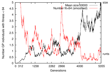
Figure 3: Evolution of low fitness in first 6-mux pop=500 run. All poor fitness trees (runts) first removed in gen 312. (Plot has been smooth over 30 generations.) After generation 312, there are at most 11 trees with fitness $<64$ (gens 1238, 2866 and one 10, gen 2262). (Mean prog size in background.)

Figure 4, (page 4) shows once a GP run has found a tree with max fitness, the impact of fitness selection on subsequent generations falls rapidly in line with theory. I.e. the expected number of tournaments $y$ using some aspect of fitness is given by $y=2\times{\rm popsize}\left(1-(1-x/{\rm popsize})^{7}\right)$ where $x$ is the number of poor fitness trees in the population and the tournament size is 7. Near the origin $y\approx 14x$. In a typical run, after first fitness convergence, two thirds of generations contain one, two or more poor children. Meaning on average in $2/3^{\rm rds}$ of populations, fitness selection plays some role in the choice of parents for 14, 28 or more children.

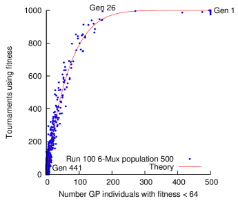
Figure 4: Convergence of typical GP population leads to reduction in fitness variation and so fewer tournaments using any aspect of fitness. Except where a population converges to fitness below 64, all runs follow the theoretical curve $2\times{\rm popsize}\left(1-(1-x/{\rm popsize})^{\rm tourn\ size}\right)$.

2.3 Introns

The functions available to evolution are AND, OR, NAND and NOR. If, for all fitness test cases, an input to an AND node is 0, then the AND’s output will also always be 0. Whereas if an input to NAND is always 0 NAND’s output is always 1. Similarly always 1 for OR gives always 1, and it gives always 0 for NOR. Our GP system does not pre-define such constants, however they can be readily evolved in many ways. E.g. 0 can be created by taking any leaf and anding it with its inverse. Given these four combinations of functions and 0 and 1, the other input to the function has no impact on the nodes output. Indeed, since our function set has no side-effects, the whole subtree leading to the input has no impact. Some GP systems may be optimised to avoid even evaluating it. Further, not only can it have no effect in the current tree, any genetic changes to it also have no effect. Meaning children who only differ from their parent in such subtrees are guaranteed to have exactly the same fitness as their parent. In genetic programming we have been calling such subtrees “introns”. Although it does not use this information, our GP system was modified to recognise and report such introns.

2.4 The Importance of Mothers

Figure 5 shows the size of low fitness children is highly correlated with the parent (mother) which they inherent their root node from. Figure 6 (left) shows that crossovers which change fitness tend to remove more code than they add but this effect is dwarfed by the factor that 90% of mothers of unsuccessful offspring are smaller than average and on average the difference is much bigger than the change in size caused by the damaging crossover, see Figure 6 (right). However (as we shall see in the next section page 2.5) in many cases the fraction of the new population with worse fitness than their mothers is far smaller than the fraction of introns and the difference is largely made up by the protection afforded by constants.

Figure 5: Size of all 6695 children (typical run) with fitness less than their parents compared to size of their parents (x-axis) which both have max fitness (64). Note strong correlation with root node parent (mum).

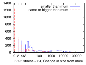
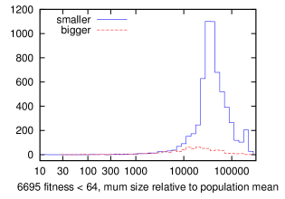
Figure 6: Left: Change in size of 6695 poor fitness children (typical run) (Decile bins used for changes bigger than 8). More than half (3428) of the children are smaller than their 1st parent, 2018 (30%) larger and 1249 (19%) the same size. Right: Distribution of size of 1st parent (mum) relative to population mean for all 6695 low fitness ($<64$) children (typical run) where both parents have max fitness (64). 90% of the mums are smaller than average. (Same data as Figure 5.)

2.5 Entropy & Evolution of Robust Constants

Although all the components in the evolved trees are deterministic they lead to progressive information loss (entropy reduction). When the components are deeply nested (i.e. the trees are large) the loss may be complete, leading to subtrees whose output is independent of their leafs. We call such zero entropy subtrees constants.

$$\mbox{Entropy is }\ \ S=-64\left(p\log_{2}(p)+q\log_{2}(q)\right)$$

where $p$ is the fraction of the 64 fitness cases which are true (and $q$ for zero). We use $\log_{2}$ so that entropy is expressed in bits. Notice in these experiments the entropy of all leafs is 64 bits and all constants have entropy of zero. With our, deliberately symmetric, function set, the entropy of a function with identical inputs is the same as that of those inputs. Whilst the entropy of a function whose inputs are two different leafs will be $S=-64\left(\frac{3}{4}\log_{2}\left(\frac{3}{4}\right)+\frac{1}{4}\log_{2}\left(\frac{1}{4}\right)\right)=51.92\ \mbox{bits}$ I.e. lower than that of either input. This is generally true of any program: the entropy of each step is typically lower than the entropy of its inputs and cannot be higher. (This is reasonable since no deterministic system can increase the information content of its input.) Another way to view this is that the impact of each leaf is diluted in each function by the effect of the leafs attached (possible indirectly) to the function’s other input. This suggests leafs in a function’s subtree but separated from it by many intermediate levels of the subtree would tend to have less impact on it. If the path from any code to the root node passes through a zero entropy function, it cannot effect the output of the tree and we call it ineffective code.

Large evolved trees contain evolved constants. For example both trees in Figure 12 (page 12) contain three constants created by OR functions. The whole of the subtree below the constant can be replaced by the constant without changing the program’s output in any way. Evolved constants are resilient to changes in the subtree beneath them. In a typical run after the first time the population converges so that everyone has maximum fitness (i.e. generation 312) only one or two crossovers made in subtrees headed by a constant reduce the child’s fitness. On average over 500 generations after generation 312, 99.6% of children are modified only in code below a constant, on average in each generation of these 1.9 (0.38% of the population) do not have maximum fitness. The remaining 0.4% of crossovers, give rise to on average 0.8 poor fitness children (0.16% of the population).

2.6 Evolution of High Fitness Within Trees

A potential alternative way for GP individuals to protect their children in the evolving population might be to contain multiple instances of high fitness code so that crossover between descendants would have some chance of copying complete high fitness code (building blocks). This would also require the insertion point to be receptive. However if we take the view that the high fitness code must itself be a subtree, then Figure 7 shows this does not happen. In all our pop=500 runs, even after thousands of generations, on average there are less than a handful of subtrees per individual which themselves have max fitness. Since they are so few they stand very little chance of being selected as a crossover point in trees of several hundred thousand nodes.

Figure 8 (page 8) shows good agreement between the observed occurrence of whole tree insertion crossovers and theory based on the size of the trees. Between gen 312 (the first time the whole population reached max fitness) and generation 1828 there were 758 500 crossovers. Based on tree sizes, about 60 should have caused the whole of one parent to be inserted into the other. Although they give rise to children which contain multiple subtrees with fitness 64 these do not spread through the population and the average number of such subtrees remains near 1.0 until much later (see Figure 7).

Figure 7: Evolution of average number of 6-mux subtrees in the population with max fitness (64) (typical GP run). Notice several thousand generations where there is almost exactly one per tree in the population. Only after extreme bloat (dotted line) do we sometimes get $>1$ subtrees with fit=64.

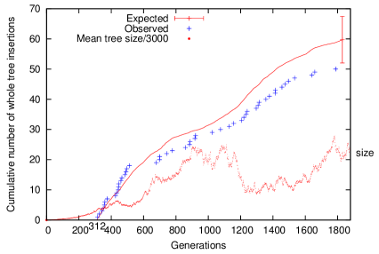
Figure 8: Count of number of whole trees inserted $+$ (i.e. crossover point at root of second parent). Showing agreement with theory (solid line). The count is started from the first time the population converges to 100% max fitness and is shown for the next 500 generations. For ease of comparison the average size of trees is shown dotted. The expected rate of increase falls as trees get bigger.

2.7 Evolution of Constants

With our [12] Boolean function set, evolution readily assembles constants and these rapidly spread through the population. The exact ratios vary between runs. (Figure 9, page 9, shows their evolution in a typical run.) After a few hundred generations, functions which evaluate to the same value for all test cases occupy a few percent of the whole population and once evolved these fractions are fairly stable to the end of the run. Such high densities of constants reflect the large fraction of introns and ineffective code in the highly evolved trees.

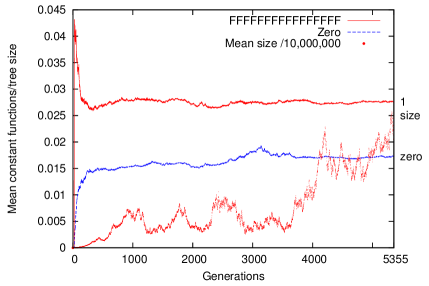
Figure 9: Evolution of average fraction of nodes in the population which evaluate to a constant (typical GP run). Notice several thousand generations where the fraction of the evolving population which are constant is almost unchanging.

2.8 Evolution of Tree Size and Depth

Figure 10 (page 10) shows the distribution of subtrees within a highly evolved population at generation 2500. As expected [18], in no case are trees either maximally short and bushy or maximally tall and thin. Instead both trees and subtrees lie near the mean size v. depth limit calculated by Flajolet for random binary trees of a given size [17]. Random trees have the fractal like property that often there is a leaf close to their root node and this is also true of subtrees within them.

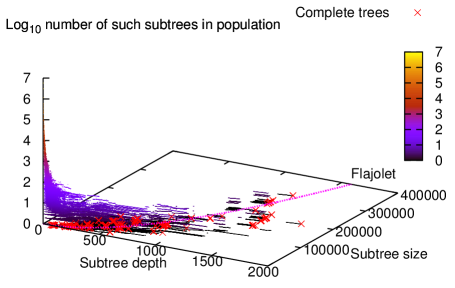
Figure 10: Generation 2500 of typical 6-mux run. Highly evolved trees ($\times$) lie close to Flajolet line (dotted parabola). As predicted their subtrees are also like random trees [18].

If we compare the evolved distribution of tree sizes with Poli’s limiting distribution [19] the match is good but the actual distribution does differ significantly from theory, see Figure 11. Nonetheless the theory does predict both the extended tail to very small trees and the upper tail. It also predicts reasonably well the location of the peak.

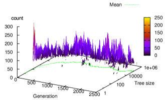
Figure 11: Distribution of highly evolved fit trees in a typical run (decile bins). Left: Generation 2500. The dotted line shows Poli’s theoretical limiting distribution for random crossover [19, Eq 24] (arity $a=2$, $p_{a}$ set to fit observed mean: 82482.1). Right: Generations 0 to 2500. Colour indicates by how much each decile bin exceeds value plus three standard deviations predicted by Poli’s limiting distribution [19]. Note log scales.

The generation (2500) depicted in Figure 11 (left) is not atypical. If we look at all generations leading up to it, after generation 35, in every case at some point one or more groups of trees have more similar sizes than predicted by unfettered random crossover (colour in Figure 11 right). Suggesting even the very modest degree of fitness selection continues to have an impact on the population (even when the trees get smaller with time). Again the distribution predicts the tails reasonable well.

2.9 Evolution of Effective Code

Figure 1 (page 1) has already shown that the size of effective code is fairly stable. Figure 12 shows the effective code in two typical trees separated by 100 generations. (I.e. at generation 400 and 500.) Notice even after 100 generations the effective part of the evolved trees is little changed. Indeed if we look at the effective code in every tree in the population at generation 500 (Figure 13 page 13) we see they are also very similar. Typically the effective part of the code lies in a few hundred nodes around the root node (yellow) which is protected against crossover by evolved constants. The constants head large sacrificial subtrees of ineffective code. Figure 13 shows the effective code is conserved over many generations. We see this in all pop=500 runs (except 102, gets stuck at fitness=62). However the details of the evolved effective code differ from run to run.

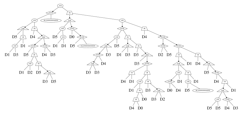
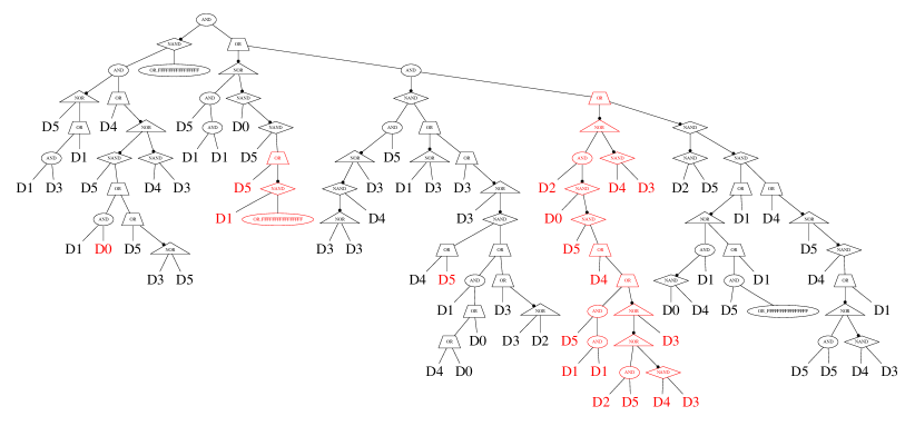
Figure 12: Typical 6-mux effective code with max fitness (64). Top: generation 400. The whole program is 15 495 instructions but only 111 are effective. Bottom: generation 500. Only the 141 effective out of 16 831 instructions shown. Notice similarity. See also Figure 13 which shows all high fitness trees in generation 500.

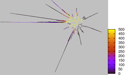
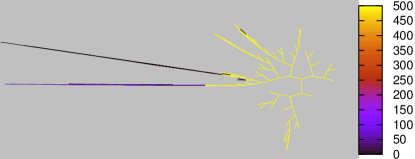
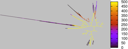
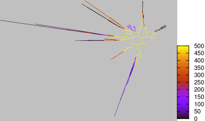
Figure 13: Effective code in a population of 500 binary trees after 500, 1000, 2000 and 4000 generations. (Each panel showing the 496-500 trees with max fitness.) Note the similarity of the effective code even though separated by thousands of generations. By generation 4000 although the trees range in size from 843 to 328 723 the effective code is limited to the 721 nodes shown (0.2% of the total). Almost all the population have 82 effective nodes in common (yellow). Darker colours indicate effective code which only occurs in $\leq$148 (blue) or $\leq$22 (black) trees. Code which does not effect any program’s output is not plotted.

3 A Limit to Bloat

Can bloat continue forever? Even in these extended runs fitness selection is needed to sustain the tree size [20], in that if we turn off selection, the number of nodes in the population executes an apparently random walk. However, a population of very small trees, represents an absorbing state from which it may take crossover a long time to escape. Indeed a population of all leafs can be constructed by crossover but it cannot escape it. The presence of an absorbing state converts the random walk into a gambler’s ruin.

Once trees become so big that the population contains no low fitness individuals, tree size executes a gamblers ruin towards zero. Although the step size increases with tree size, it appears highly unlikely for the population to migrate to tiny trees which crossover cannot escape, without transitioning through a regime where small trees have low fitness and hence fitness selection will kick back in to grow the trees again.

We speculate that in a finite population it will become possible that the bloated trees become so large that in any generation the expected number of times crossover disrupts the high fitness core near the root node falls well below one per generation Thus removing the driving force which has been growing the trees. Hence their may be a balancing point with the gambler’s ruin near

$$\mbox{tree size}\approx{\rm popsize}\times\mbox{core codesize}$$

In the above experiments $500\times 497=248\,500$.

Figure 14 (page 14) shows ten extended runs with a reduced population size and no size limits. The smaller population size means GP is usually no longer able to solve the problem nevertheless as expected the run shows similar characteristics to the larger population. The size of the core code is not known but we would anticipate it would be no bigger than in runs where high fitness trees do evolve. Thus we had anticipated an edge to bloat at about 25 000. All ten extended runs with the small population behaved similarly. They all bloated (max tree size between 3 600 000 and 115 000 000) but at the end of each run the average tree size was between 0.01% and 6% of the maximum tree size. (Only two runs reach max fitness 64.) Across ten runs and over 100 000 generations the median mean tree size in the population was 42 507 and the median smallest was 10 513.

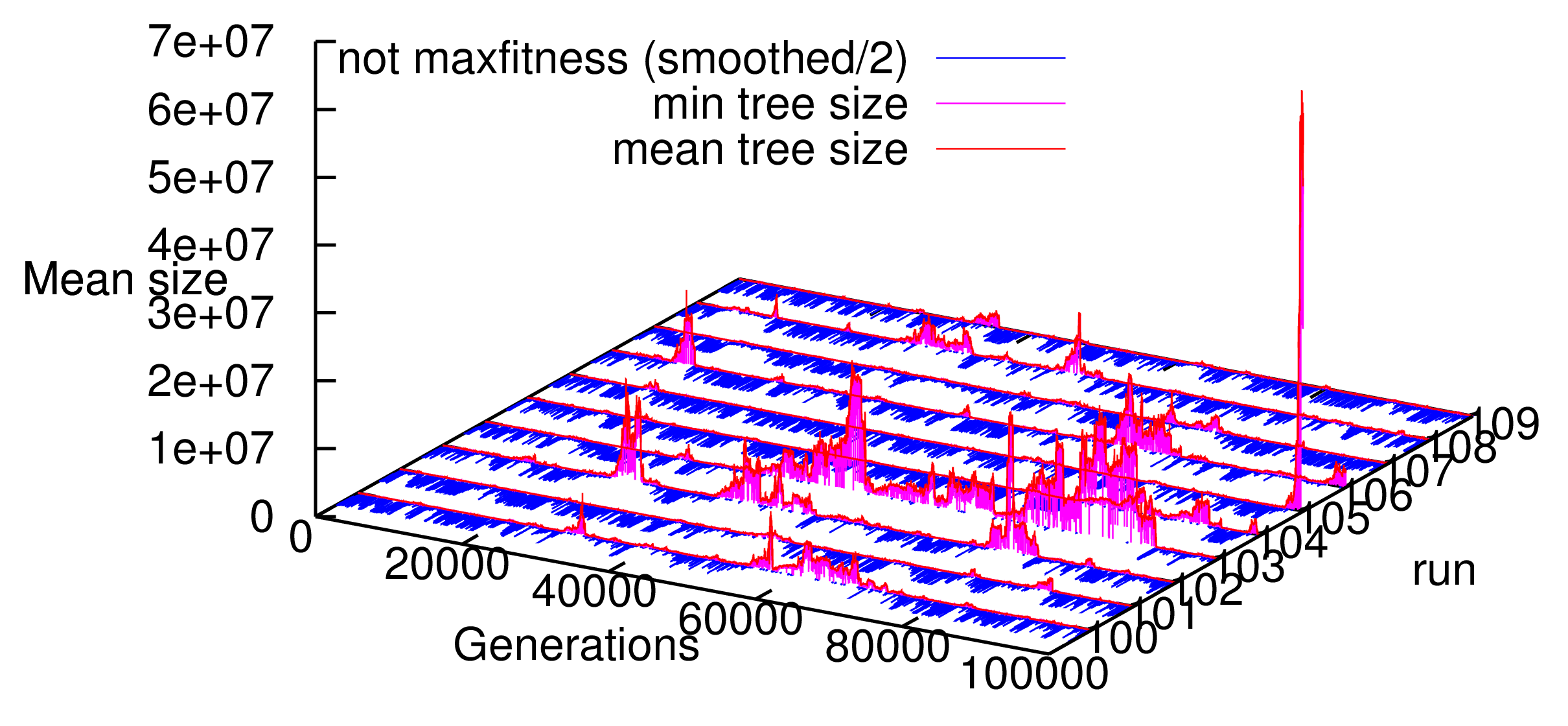
Figure 14: Extended runs pop=50. Blue horizontal curve shows number of GP individuals with fitness $<64$ (rescaled by 0.5 and smoothed). In populations with huge trees, even the smallest tree is big and in many gens whole pop has same fitness. Without a fitness differential, tree size may rise or fall.

4 Conclusions

We have studied long term evolution (far longer than anything reported in GP). In our populations after thousands, even tens of thousands, of generations trees evolve to be extremely stable so that there may be tens or even hundreds of generations where everyone has the same fitness. This means that there is no selection and we see bloat become an apparently random walk, with both increases and falls in program size. Further we suggest, in finite populations, bloat is naturally limited by a gambler’s ruin process.

The evolved (albeit narrowly defined) introns do not explain the extreme fitness convergence seen. Instead we have described the evolution of functions with constant output (zero entropy). These shelter the root node and are evolved to be resilient to crossover.

The evolved constants form a protective ring around highly stable effective code centred on the root node and head huge sacrificial subtrees of ineffective code. (These may contain 100 000s of useless instructions.) This ineffective code is primarily responsible for the low number of low fitness individuals found in highly evolved populations.

Even after evolving for thousands of generations, in small populations, we continue to see the impact of fitness selection on the distribution of tree sizes. And, although the distribution of tree sizes versus their depths is close to that of random trees, the distribution of tree sizes does not approach the limiting distribution we predicted assuming no fitness [19].

GP code available via anonymous FTP and http://www.cs.ucl.ac.uk/staff/W.Langdon/ftp/ gp-code/GPbmux6.tar.gz

References

- [1] Lenski, R.E., et al.: Sustained fitness gains and variability in fitness trajectories in the long-term evolution experiment with Escherichia coli. Proceedings of the Royal Society B 282(1821) (2015)
- [2] Koza, J.R.: Genetic Programming MIT press (1992)
- [3] Banzhaf, W., Nordin, P., Keller, R.E., Francone, F.D.: Genetic Programming -- An Introduction (1998)
- [4] Poli, R., Langdon, W.B., McPhee, N.F.: A field guide to genetic programming. (2008)
- [5] Tackett, W.A.: Recombination, Selection, and the Genetic Construction of Computer Programs. PhD thesis, University of Southern California (1994)
- [6] Altenberg, L.: The evolution of evolvability in genetic programming. In Advances in GP. MIT Press (1994)
- [7] Angeline, P.J.: Genetic programming and emergent intelligence. In Advances in GP. MIT Press (1994)
- [8] Langdon, W.B.: Size fair and homologous tree genetic programming crossovers. GP&EM 1(1/2) 95--119
- [9] Harvey, I.: Open the box. Position paper at the Workshop on Evolutionary Computation with Variable Size Representation at ICGA-97 (1997)
- [10] Lewis, T.E., Magoulas, G.D.: Tweaking a tower of blocks leads to a TMBL: Pursuing long term fitness growth in program evolution. CEC 2010, 4465--4472
- [11] McPhee, N.F., Poli, R.: A schema theory analysis of the evolution of size in genetic programming with linear representations. In EuroGP’2001, 108--125
- [12] Langdon, W.B.: Quadratic bloat in genetic programming. In GECCO-2000, 451--458
- [13] Poli, R., Langdon, W.B.: Sub-machine-code genetic programming. In Advances in GP 3. (1999) 301--323
- [14] Nordin, P.: Evolutionary Program Induction of Binary Machine Code and its Applications. PhD thesis, der Universitat Dortmund (1997)
- [15] Stephens, C., Waelbroeck, H.: Schemata evolution and building blocks. Evo. Comp. 7(2) (1999) 109--124
- [16] Langdon, W.B., Poli, R.: Foundations of Genetic Programming. Springer-Verlag (2002)
- [17] Flajolet, P., Oldyzko, A.: The average height of binary trees and other simple trees. JCSS 25 (1982) 171--213
- [18] Langdon, W.B.: Scaling of program tree fitness spaces. Evolutionary Computation 7(4) (1999) 399--428
- [19] Poli, R., Langdon, W.B., Dignum, S.: On the limiting distribution of program sizes in tree-based genetic programming. In EuroGP-2007. 193--204
- [20] Langdon, W.B., Poli, R.: Fitness causes bloat. In Chawdhry, P.K., et al., eds.: Soft Comp. in Eng. Design and Manufacturing, Springer (1997) 13--22
- [21] Langdon, W.B. In: GECCO, Berlin (2017).