Fault Detection and Isolation Tools (FDITOOLS)

User’s Guide

Abstract

The Fault Detection and Isolation Tools (FDITOOLS) is a collection of MATLAB functions for the analysis and solution of fault detection and model detection problems. The implemented functions are based on the computational procedures described in the Chapters 5, 6 and 7 of the book: ”A. Varga, Solving Fault Diagnosis Problems – Linear Synthesis Techniques, Springer, 2017”. This document is the User’s Guide for the version V1.0 of FDITOOLS. First, we present the mathematical background for solving several basic exact and approximate synthesis problems of fault detection filters and model detection filters. Then, we give in-depth information on the command syntax of the main analysis and synthesis functions. Several examples illustrate the use of the main functions of FDITOOLS.

Cont.1Cont.1ContentsContentsCont.1

Notations and Symbols

General notations

$\mathds{C}$	field of complex numbers
$\mathds{R}$	field of real numbers
$\mathds{C}_{s}$	stability domain (i.e., open left complex half-plane in continuous-time or open unit disk centered in the origin in discrete-time)
$\partial\mathds{C}_{s}$	boundary of stability domain (i.e., extended imaginary axis with infinity included in continuous-time, or unit circle centered in the origin in discrete-time)
$\overline{\mathds{C}}_{s}$	closure of $\mathds{C}_{s}$: $\overline{\mathds{C}}_{s}=\mathds{C}_{s}\cup\partial\mathds{C}_{s}$
${\mathds{C}}_{u}$	open instability domain: $\mathds{C}_{u}:=\mathds{C}\setminus\overline{\mathds{C}}_{s}$
$\overline{\mathds{C}}_{u}$	closure of ${\mathds{C}}_{u}$: $\overline{\mathds{C}}_{u}:=\mathds{C}_{u}\cup\partial\mathds{C}_{s}$
$\mathds{C}_{g}$	“good” domain of $\mathds{C}$
$\mathds{C}_{b}$	“bad” domain of $\mathds{C}$: $\mathds{C}_{b}=\mathds{C}\setminus\mathds{C}_{g}$
$s$	complex frequency variable in the Laplace transform: $s=\sigma+\mathrm{i}\omega$
$z$	complex frequency variable in the Z-transform: $z=\mathrm{e}^{\,sT}$, $T$ – sampling time
$\lambda$	complex frequency variable: $\lambda=s$ in continuous-time or $\lambda=z$ in discrete-time
$\bar{\lambda}$	complex conjugate of the complex number $\lambda$
$\mathds{R}(\lambda)$	set of rational matrices in indeterminate $\lambda$ with real coefficients
$\mathds{R}(\lambda)^{p\times m}$	set of $p\times m$ rational matrices in indeterminate $\lambda$ with real coefficients
$\delta(G(\lambda))$	McMillan degree of the rational matrix $G(\lambda)$
$G^{\sim}(\lambda)$	Conjugate of $G(\lambda)\in\mathds{R}(\lambda)$: $G^{\sim}(s)=G^{T}(-s)$ in continuous-time and $G^{\sim}(z)=G^{T}(1/z)$ in discrete-time
$\ell_{2}$	Banach-space of square-summable sequences
$\mathcal{L}_{2}$	Lebesgue-space of square-integrable functions
$\mathcal{L}_{\infty}$	Space of complex-valued functions bounded and analytic in ${\partial\mathds{C}}_{s}$
$\mathcal{H}_{\infty}$	Hardy-space of complex-valued functions bounded and analytic in ${\mathds{C}}_{u}$
$\|G\|_{2}$	$\mathcal{H}_{2}$- or $\mathcal{L}_{2}$-norm of the transfer function matrix $G(\lambda)$ or 2-norm of a matrix $G$
$\|G\|_{\infty}$	$\mathcal{H}_{\infty}$- or $\mathcal{L}_{\infty}$-norm of the transfer function matrix $G(\lambda)$
$\|G\|_{\infty/2}$	either the $\mathcal{H}_{\infty}$- or $\mathcal{H}_{2}$-norm of the transfer function matrix $G(\lambda)$
$\|G\|_{\infty-}$	$\mathcal{H}_{\infty-}$-index of the transfer function matrix $G(\lambda)$
$\|G\|_{\Omega-}$	$\mathcal{H}_{-}$-index over a frequency domain $\Omega$ of the transfer function matrix $G(\lambda)$
$\delta_{\nu}(G_{1},G_{2})$	$\nu$-gap distance between the transfer function matrices $G_{1}(\lambda)$ and $G_{2}(\lambda)$
$M^{T}$	transpose of the matrix $M$
$M^{-1}$	inverse of the matrix $M$
$M^{-L}$	left inverse of the matrix $M$
$\overline{\sigma}(M)$	largest singular value of the matrix $M$
$\underline{\sigma}(M)$	least singular value of the matrix $M$
$\mathcal{N}(M)$	kernel (or right nullspace) of the matrix $M$
$\mathcal{N}_{L}(G(\lambda))$	left kernel (or left nullspace) of $G(\lambda)\in\mathds{R}(\lambda)$
$\mathcal{N}_{R}(G(\lambda))$	right kernel (or right nullspace) of $G(\lambda)\in\mathds{R}(\lambda)$
$\mathcal{R}(M)$	range (or image space) of the matrix $M$
$I_{n}$ or $I$	identity matrix of order $n$ or of an order resulting from context
$e_{i}$	the $i$-th column of the (known size) identity matrix
$0_{m\times n}$ or $0$	zero matrix of size ${m\times n}$ or of a size resulting from context

Fault diagnosis related notations

$y(t)$	measured output vector: $y(t)\in\mathds{R}^{p}$
$\mathbf{y}(\lambda)$	Laplace- or $\mathcal{Z}$-transformed measured output vector
$u(t)$	control input vector: $u(t)\in\mathds{R}^{m_{u}}$
$\mathbf{u}(\lambda)$	Laplace- or $\mathcal{Z}$-transformed control input vector
$d(t)$	disturbance input vector: $d(t)\in\mathds{R}^{m_{d}}$
$\mathbf{d}(\lambda)$	Laplace- or $\mathcal{Z}$-transformed disturbance input vector
$w(t)$	noise input vector: $w(t)\in\mathds{R}^{m_{w}}$
$\mathbf{w}(\lambda)$	Laplace- or $\mathcal{Z}$-transformed noise input vector
$f(t)$	fault input vector: $f(t)\in\mathds{R}^{m_{f}}$
$\mathbf{f}(\lambda)$	Laplace- or $\mathcal{Z}$-transformed fault input vector
$x(t)$	state vector: $x(t)\in\mathds{R}^{n}$
$G_{u}(\lambda)$	transfer function matrix from $u$ to $y$
$G_{d}(\lambda)$	transfer function matrix from $d$ to $y$
$G_{w}(\lambda)$	transfer function matrix from $w$ to $y$
$G_{f}(\lambda)$	transfer function matrix from $f$ to $y$
$G_{f_{j}}(\lambda)$	transfer function matrix from the $j$-th fault input $f_{j}$ to $y$
$A$	system state matrix
$E$	system descriptor matrix
$B_{u}$, $B_{d}$, $B_{w}$, $B_{f}$	system input matrices from $u$, $d$, $w$, $f$
$C$	system output matrix
$D_{u}$, $D_{d}$, $D_{w}$, $D_{f}$	system feedthrough matrices from $u$, $d$, $w$, $f$
$r(t)$	residual vector: $r(t)\in\mathds{R}^{q}$
$\mathbf{r}(\lambda)$	Laplace- or $\mathcal{Z}$-transformed residual vector
$n_{b}$	number of components of residual vector $r$
$r^{(i)}(t)$	$i$-th residual vector component: $r^{(i)}(t)\in\mathds{R}^{q_{i}}$
$\mathbf{r}^{(i)}(\lambda)$	Laplace- or $\mathcal{Z}$-transformed $i$-th residual vector component
$Q(\lambda)$	transfer function matrix of the implementation form of the residual generator from $y$ and $u$ to $r$
$Q_{y}(\lambda)$	transfer function matrix of residual generator from $y$ to $r$
$Q_{u}(\lambda)$	transfer function matrix of residual generator from $u$ to $r$
$Q^{(i)}(\lambda)$	transfer function matrix of the implementation form of the $i$-th residual generator from $y$ and $u$ to $r^{(i)}$
$R(\lambda)$	transfer function matrix of the internal form of the residual generator from $u$, $d$, $w$ and $f$ to $r$
$R_{u}(\lambda)$	transfer function matrix from $u$ to $r$
$R_{d}(\lambda)$	transfer function matrix from $d$ to $r$
$R_{w}(\lambda)$	transfer function matrix from $w$ to $r$
$R_{f}(\lambda)$	transfer function matrix from $f$ to $r$
$R_{f_{j}}(\lambda)$	transfer function matrix from the $j$-th fault input $f_{j}$ to $r$
$R^{(i)}_{f_{j}}(\lambda)$	transfer function matrix from the $j$-th fault input $f_{j}$ to $r^{(i)}$
$S$	binary structure matrix
$S_{R_{f}}$	binary structure matrix corresponding to $R_{f}(\lambda)$
$M_{r}(\lambda)$	transfer function matrix of a reference model from $f$ to $r$
$\theta(t)$	residual evaluation vector
$\iota(t)$	binary decision vector
$\tau$, $\tau_{i}$	decision thresholds

Model detection related notations

$N$	number of component models of the multiple model
$y(t)$	measured output vector: $y(t)\in\mathds{R}^{p}$
$\mathbf{y}(\lambda)$	Laplace- or $\mathcal{Z}$-transformed measured output vector
$u(t)$	control input vector: $u(t)\in\mathds{R}^{m_{u}}$
$\mathbf{u}(\lambda)$	Laplace- or $\mathcal{Z}$-transformed control input vector
$u^{(j)}(t)$	control input vector of $j$-th model: $u^{(j)}(t):=u(t)\in\mathds{R}^{m_{u}}$
$\mathbf{u}^{(j)}(\lambda)$	Laplace- or $\mathcal{Z}$-transformed control input vector of $j$-th model
$d^{(j)}(t)$	disturbance input vector of $j$-th model: $d^{(j)}(t)\in\mathds{R}^{m_{d}^{(j)}}$
$\mathbf{d}^{(j)}(\lambda)$	Laplace- or $\mathcal{Z}$-transformed disturbance input vector of $j$-th model
$w^{(j)}(t)$	noise input vector of $j$-th model: $w^{(j)}(t)\in\mathds{R}^{m_{w}^{(j)}}$
$\mathbf{w}^{(j)}(\lambda)$	Laplace- or $\mathcal{Z}$-transformed noise input vector of $j$-th model
$y^{(j)}(t)$	output vector of $j$-th model: $y^{(j)}(t)\in\mathds{R}^{p}$
$\mathbf{y}^{(j)}(\lambda)$	Laplace- or $\mathcal{Z}$-transformed output vector of $j$-th model
$x^{(j)}(t)$	state vector of $j$-th model: $x^{(j)}(t)\in\mathds{R}^{n_{i}}$
$G_{u}^{(j)}(\lambda)$	transfer function matrix of $j$-th model from $u^{(j)}$ to $y^{(j)}$
$G_{d}^{(j)}(\lambda)$	transfer function matrix of $j$-th model from $d^{(j)}$ to $y^{(j)}$
$G_{w}^{(j)}(\lambda)$	transfer function matrix of $j$-th model from $w^{(j)}$ to $y^{(j)}$
$A^{(j)}$	system state matrix of $j$-th model
$E^{(j)}$	system descriptor matrix of $j$-th model
$B_{u}^{(j)}$, $B_{d}^{(j)}$, $B_{w}^{(j)}$	system input matrices of $j$-th model from $u^{(j)}\!$, $d^{(j)}\!$, $w^{(j)}$
$C^{(j)}$	system output matrix of $j$-th model
$D_{u}^{(j)}$, $D_{d}^{(j)}$, $D_{w}^{(j)}$	system feedthrough matrices of $j$-th model from $u^{(j)}\!$, $d^{(j)}\!$, $w^{(j)}$
$r^{(i)}(t)$	$i$-th residual vector component: $r^{(i)}(t)\in\mathds{R}^{q_{i}}$
$\mathbf{r}^{(i)}(\lambda)$	Laplace- or $\mathcal{Z}$-transformed $i$-th residual vector component
$r(t)$	overall residual vector: $r(t)\in\mathds{R}^{q}$, $q=\sum_{i=1}^{N}q_{i}$
$\mathbf{r}(\lambda)$	Laplace- or $\mathcal{Z}$-transformed overall residual vector
$Q^{(i)}(\lambda)$	transfer function matrix of the implementation form of the $i$-th residual generator from $y$ and $u$ to $r^{(i)}$
$Q_{y}^{(i)}(\lambda)$	transfer function matrix of residual generator from $y$ to $r^{(i)}$
$Q_{u}^{(i)}(\lambda)$	transfer function matrix of residual generator from $u$ to $r^{(i)}$
$Q(\lambda)$	transfer function matrix of the implementation form of the overall residual generator from $y$ and $u$ to $r$
$R^{(i,j)}(\lambda)$	the transfer function matrix of the internal form of the overall residual generator from $(u^{(j)}\!,d^{(j)}\!,w^{(j)})$ to $r^{(i)}$
$R_{u}^{(i,j)}(\lambda)$	the transfer function matrix of the internal form of the overall residual generator from $u^{(j)}$ to $r^{(i)}$
$R_{d}^{(i,j)}(\lambda)$	the transfer function matrix of the internal form of the overall residual generator from $d^{(j)}$ to $r^{(i)}$
$R_{w}^{(i,j)}(\lambda)$	the transfer function matrix of the internal form of the overall residual generator from $w^{(j)}$ to $r^{(i)}$
$\theta(t)$	$N$-dimensional residual evaluation vector
$\iota(t)$	$N$-dimensional binary decision vector
$\tau_{i}$	decision threshold for $i$-th component of the residual vector

Acronyms

AFDP	Approximate fault detection problem
AFDIP	Approximate fault detection and isolation problem
AMDP	Approximate model detection problem
AMMP	Approximate model matching problem
EFDP	Exact fault detection problem
EFEP	Exact fault estimation problem
EFDIP	Exact fault detection and isolation problem
EMDP	Exact model detection problem
EMMP	Exact model matching problem
FDD	Fault detection and diagnosis
FDI	Fault detection and isolation
LTI	Linear time-invariant
LFT	Linear fractional transformation
LPV	Linear parameter-varying
MIMO	Multiple-input multiple-output
MMP	Model-matching problem
TFM	Transfer function matrix

1 Introduction

The Fault Detection and Isolation Tools (FDITOOLS) is a collection of MATLAB functions for the analysis and solution of fault detection problems. FDITOOLS supports various synthesis approaches of linear residual generation filters for continuous- or discrete-time linear systems. The underlying synthesis techniques rely on reliable numerical algorithms developed by the author and described in the Chapters 5, 6 and 7 of the author’s book [16]:

Andreas Varga, Solving Fault Diagnosis Problems - Linear Synthesis Techniques,
vol. 84 of Studies in Systems, Decision and Control, Springer International Publishing,
xxviii+394, 2017.

The functions of the FDITOOLS collection rely on the Control System Toolbox [2] and the Descriptor System Tools (DSTOOLS) V0.71 [4]. The current release of FDITOOLS is version V1.0, dated November 30, 2018. FDITOOLS is distributed as a free software via the Bitbucket repository. The codes have been developed under MATLAB 2015b and have been also tested with MATLAB 2016a through 2018b. To use the functions of FDITOOLS, the Control System Toolbox and the DSTOOLS collection must be installed in MATLAB running under 64-bit Windows 7, 8, 8.1 or 10.

This document describes version V1.0 of the FDITOOLS collection. This version covers all synthesis procedures described in the book [16] and, additionally, includes a comprehensive collection of analysis functions, as well as functions for an easy setup of synthesis models. The book [16] represents an important complementary documentation for the FDITOOLS collection: it describes the mathematical background of solving synthesis problems of fault detection and model detection filters and gives detailed descriptions of the underlying synthesis procedures. Additionally, the M-files of the functions are self-documenting and a detailed documentation can be obtained online by typing help with the M-file name. Please cite FDITOOLS as follows:

A. Varga. FDITOOLS – The Fault Detection and Isolation Tools for MATLAB, 2018.

https://sites.google.com/site/andreasvargacontact/home/software/fditools.

The implementation of the functions included in the FDITOOLS collection follows several principles, which have been consequently enforced when implementing these functions. These principles are listed below and partly consists of the requirements for robust software implementation, but also include several requirements which are specific to the field of fault detection:

• Using general, numerically reliable and computationally efficient numerical approaches as basis for the implementation of all computational functions, to guarantee the solvability of problems under the most general existence conditions of the solutions. Consequently, the implemented methods provide a solution whenever a solution exists. These methods are extensively described in the book [16], which forms the methodological and computational basis of all implemented analysis and synthesis functions.

• Support for the most general model representation of linear time-invariant systems in form of generalized state-space representation, also known as descriptor systems. All analysis and synthesis functions are applicable to both continuous- and discrete-time systems. The basis for implementation of all functions is the Descriptor System Tools (DSTOOLS) [4], a collection of functions to handle rational transfer function matrices (proper or improper), via their equivalent descriptor system representations. The initial version of this collection has been implemented in conjunction with the book [16].

• Providing simple user interface to all synthesis functions. All functions rely on default settings of problem parameters and synthesis options, which allow to easily obtain preliminary synthesis results. Also, all functions to solve a class of problems (e.g., fault detection), are applicable to the same input models. Therefore, the synthesis functions to solve approximate synthesis problems are applicable to solve the exact synthesis problems as well. On the other side, the solution of an exact problem for a system with noise inputs, represents a first approximation to the solution of the approximate synthesis problem.

• Providing an exhaustive set of options to ensure the complete freedom in choosing problem specific parameter and synthesis options. Among the frequently used synthesis options are: the number of residual signal outputs or the numbers of outputs of the components of structured residual signals; stability degree for the poles of the resulting filters or the location of their poles; frequency values to enforce strong fault detectability; type of the employed nullspace basis (e.g., proper, proper and simple, full-order observer); performing least-order synthesis, etc.

• Guaranteeing the reproducibility of results. This feature is enforced by employing the so-called design matrices. These matrices are internally used to build linear combinations of left nullspace basis vectors and are frequently randomly generated (if not explicitly provided). The values of the employed design matrices are returned as additional information by all synthesis functions. The use of design matrices also represents a convenient mean to perform an optimization-based tuning of these matrices to achieve specific performance characteristics for the resulting filters.

2 Fault Detection Basics

In this section we describe first the basic fault monitoring tasks, such as fault detection and fault isolation, and then introduce and characterize the concepts of fault detectability and fault isolability. Six “canonical” fault detection problems are formulated in the book [16] for the class of linear time-invariant (LTI) systems with additive faults. Of the formulated six problems, three involve the exact synthesis and three involve the approximate synthesis of fault detection filters. The current release of FDITOOLS covers all synthesis techniques described in [16]. Jointly with the formulation of the fault detection problems, general solvability conditions are given for each problem in terms of ranks of certain transfer function matrices. More details and the proofs of the results are available in Chapters 2 and 3 of [16].

2.1 Basic Fault Monitoring Tasks

A fault represents a deviation from the normal behaviour of a system due to an unexpected event (e.g., physical component failure or supply breakdown). The occurrence of faults must be detected as early as possible to prevent any serious consequence. For this purpose, fault diagnosis techniques are used to allow the detection of occurrence of faults (fault detection) and the localization of detected faults (fault isolation). The term fault detection and diagnosis (FDD) includes the requirements for fault detection and isolation (FDI).

A FDD system is a device (usually based on a collection of real-time processing algorithms) suitably set-up to fulfill the above tasks. The minimal functionality of any FDD system is illustrated in Fig. 1.

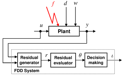
Figure 1: Basic fault diagnosis setup.

The main plant variables are the control inputs $u$, the unknown disturbance inputs $d$, the noise inputs $w$, and the output measurements $y$. The output $y$ and control input $u$ are the only measurable signals which can be used for fault monitoring purposes. The disturbance inputs $d$ and noise inputs $w$ are non-measurable “unknown” input signals, which act adversely on the system performance. For example, the unknown disturbance inputs $d$ may represent physical disturbance inputs, as for example, wind turbulence acting on an aircraft or external loads acting on a plant. Typical noise inputs are sensor noise signals as well as process input noise. However, fictive noise inputs can also account for the cumulative effects of unmodelled system dynamics or for the effects of parametric uncertainties. In general, there is no clear-cut separation between disturbances and noise, and therefore, the appropriate definition of the disturbance and noise inputs is a challenging aspect when modelling systems for solving fault detection problems. A fault is any unexpected variation of some physical parameters or variables of a plant causing an unacceptable violation of certain specification limits for normal operation. Frequently, a fault input $f$ is defined to account for any anomalous behaviour of the plant.

The main component of any FDD system (as that in Fig. 1) is the residual generator (or fault detection filter, or simply fault detector), which produces residual signals grouped in a $q$-dimensional vector $r$ by processing the available measurements $y$ and the known values of control inputs $u$. The role of the residual signals is to indicate the presence or absence of faults, and therefore the residual $r$ must be equal (or close) to zero in the absence of faults and significantly different from zero after a fault occurs. For decision-making, suitable measures of the residual magnitudes (e.g., signal norms) are generated in a vector $\theta$, which is then used to produce the corresponding decision vector $\iota$. In what follows, two basic fault monitoring tasks are formulated and discussed.

Fault detection is simply a binary decision on the presence of any fault ($f\not=0$) or the absence of all faults ($f=0$). Typically, $\theta(t)$ is scalar evaluation signal, which approximates $\|r\|_{2}$, the $\mathcal{L}_{2}$- or $\ell_{2}$-norms of signal $r$, while $\iota(t)$ is a scalar decision making signal defined as $\iota(t)=1$ if $\theta(t)>\tau$ (fault occurrence) or $\iota(t)=0$ if $\theta(t)\leq\tau$ (no fault), where $\tau$ is a suitable threshold quantifying the gap between the “small” and “large” magnitudes of the residual. The decision on the occurrence or absence of faults must be done in the presence of arbitrary control inputs $u$, disturbance inputs $d$, and noise inputs $w$ acting simultaneously on the system. The effects of the control inputs on the residual can be always decoupled by a suitable choice of the residual generation filter. In the ideal case, when no noise inputs are present ($w\equiv 0$), the residual generation filter must additionally be able to exactly decouple the effects of the disturbances inputs in the residual and ensure, simultaneously, the sensitivity of the residual to all faults (i.e., complete fault detectability, see Section 2.4). In this case, $\tau=0$ can be (ideally) used. However, in the general case when $w\not\equiv 0$, only an approximate decoupling of $w$ can be achieved (at best) and a sufficient gap must exist between the magnitudes of residuals in fault-free and faulty situations. Therefore, an appropriate choice of $\tau>0$ must avoid false alarms and missed detections.

Fault isolation concerns with the exact localization of occurred faults and involves for each component $f_{j}$ of the fault vector $f$ the decision on the presence of $j$-th fault ($f_{j}\not=0$) or its absence ($f_{j}=0$). Ideally, this must be achieved regardless the faults occur one at a time or several faults occur simultaneously. Therefore, the fault isolation task is significantly more difficult than the simpler fault detection. For fault isolation purposes, we will assume a partitioning of the $q$-dimensional residual vector $r$ in $n_{b}$ stacked $q_{i}$-dimensional subvectors $r^{(i)}$, $i=1,\ldots,n_{b}$, in the form

$$r=\left[\begin{array}[]{c}r^{(1)}\\ \vdots\\ r^{(n_{b})}\end{array}\right]\,,$$ (1)

where $q=\sum_{i=1}^{n_{b}}q_{i}$. A typical fault evaluation setup used for fault isolation is to define $\theta_{i}(t)$, the $i$-th component of $\theta(t)$, as a real-time computable approximation of $\|r^{(i)}\|_{2}$. The $i$-th component of $\iota(t)$ is set to $\iota_{i}(t)=1$ if $\theta_{i}(t)>\tau_{i}$ ($i$-th residual fired) or $\iota_{i}(t)=0$ if $\theta_{i}(t)\leq\tau_{i}$ ($i$-th residual not fired), where $\tau_{i}$ is a suitable threshold for the $i$-th subvector $r^{(i)}(t)$. If a sufficiently large number of measurements are available, then it can be aimed that $r^{(i)}$ is influenced only by the $i$-th fault signal $f_{i}$. This setting, with $n_{b}$ chosen equal to the actual number of fault components, allows strong fault isolation, where an arbitrary number of simultaneous faults can be isolated. The isolation of the $i$-th fault is achieved if $\iota_{i}(t)=1$, while for $\iota_{i}(t)=0$ the $i$-th fault is not present. In many practical applications, the lack of a sufficiently large number of measurements impedes strong isolation of simultaneous faults. Therefore, often only weak fault isolation can be performed under simplifying assumptions as, for example, that the faults occur one at a time or no more than two faults may occur simultaneously. The fault isolation schemes providing weak fault isolation compare the resulting $n_{b}$-dimensional binary decision vector $\iota(t)$, with a predefined set of binary fault signatures. If each individual fault $f_{j}$ has associated a distinct signature $s_{j}$, then the $j$-th fault can be isolated by simply checking that $\iota(t)$ matches the associated signature $s_{j}$. Similarly to fault detection, besides the decoupling of the control inputs $u$ from the residual $r$ (always possible), the exact decoupling of the disturbance inputs $d$ from $r$ can be strived in the case when $w\equiv 0$. However, in the general case when $w\not\equiv 0$, only approximate decoupling of $w$ can be achieved (at best) and a careful selection of tolerances $\tau_{i}$ is necessary to perform fault isolation without false alarms and missed detections.

2.2 Plant Models with Additive Faults

The following input-output representation is used to describe LTI systems with additive faults

$${\mathbf{y}}(\lambda)=G_{u}(\lambda){\mathbf{u}}(\lambda)+G_{d}(\lambda){\mathbf{d}}(\lambda)+G_{f}(\lambda){\mathbf{f}}(\lambda)+G_{w}(\lambda){\mathbf{w}}(\lambda),$$ (2)

where ${\mathbf{y}}(\lambda)$, ${\mathbf{u}}(\lambda)$, ${\mathbf{d}}(\lambda)$, ${\mathbf{f}}(\lambda)$, and ${\mathbf{w}}(\lambda)$, with boldface notation, denote the Laplace-transformed (in the continuous-time case) or Z-transformed (in the discrete-time case) time-dependent vectors, namely, the $p$-dimensional system output vector $y(t)$, $m_{u}$-dimensional control input vector $u(t)$, $m_{d}$-dimensional disturbance vector $d(t)$, $m_{f}$-dimensional fault vector $f(t)$, and $m_{w}$-dimensional noise vector $w(t)$ respectively. $G_{u}(\lambda)$, $G_{d}(\lambda)$, $G_{f}(\lambda)$ and $G_{w}(\lambda)$ are the transfer-function matrices (TFMs) from the control inputs $u$, disturbance inputs $d$, fault inputs $f$, and noise inputs $w$ to the outputs $y$, respectively. According to the system type, $\lambda=s$, the complex variable in the Laplace-transform in the case of a continuous-time system or $\lambda=z$, the complex variable in the Z-transform in the case of a discrete-time system. For most of practical applications, the TFMs $G_{u}(\lambda)$, $G_{d}(\lambda)$, $G_{f}(\lambda)$, and $G_{w}(\lambda)$ are proper rational matrices. However, for complete generality of our problem settings, we will allow that these TFMs are general improper rational matrices for which we will not a priori assume any further properties (e.g., stability, full rank, etc.).

The main difference between the disturbance input $d(t)$ and noise input $w(t)$ arises from the formulation of the fault monitoring goals. In this respect, when synthesizing devices to serve for fault diagnosis purposes, we will generally target the exact decoupling of the effects of disturbance inputs. Since generally the exact decoupling of effects of noise inputs is not achievable, we will simultaneously try to attenuate their effects, to achieve an approximate decoupling. Consequently, we will try to solve synthesis problems exactly or approximately, in accordance with the absence or presence of noise inputs in the underlying plant model, respectively.

An equivalent descriptor state-space realization of the input-output model (2) has the form

$$E\lambda x(t) =Ax(t)+B_{u}u(t)+B_{d}d(t)+B_{f}f(t)+B_{w}w(t)\,,$$ (3)

$$y(t) =Cx(t)+D_{u}u(t)+D_{d}d(t)+D_{f}f(t)+D_{w}w(t)\,,$$

with the $n$-dimensional state vector $x(t)$, where $\lambda x(t)=\dot{x}(t)$ or $\lambda x(t)=x(t+1)$ depending on the type of the system, continuous- or discrete-time, respectively. In general, the square matrix $E$ can be singular, but we will assume that the linear pencil $A-\lambda E$ is regular. For systems with proper TFMs in (2), we can always choose a standard state-space realization where $E=I$. In general, it is advantageous to choose the representation (3) minimal, with the pair $(A-\lambda E,C)$ observable and the pair $(A-\lambda E,[\,B_{u}\;B_{d}\;B_{f}\;B_{w}\,])$ controllable. The corresponding TFMs of the model in (2) are

$$G_{u}(\lambda) =C(\lambda E-A)^{-1}B_{u}+D_{u},$$ (4)

$$G_{d}(\lambda) =C(\lambda E-A)^{-1}B_{d}+D_{d},$$

$$G_{f}(\lambda) =C(\lambda E-A)^{-1}B_{f}+D_{f},$$

$$G_{w}(\lambda) =C(\lambda E-A)^{-1}B_{w}+D_{w}$$

or in an equivalent notation

$$\left[\begin{array}[]{cccc}G_{u}(\lambda)&G_{d}(\lambda)&G_{f}(\lambda)&G_{w}(\lambda)\end{array}\right]:={\left[\begin{array}[]{c|cccc}A-\lambda E&B_{u}&B_{d}&B_{f}&B_{w}\\ \hline\cr C&D_{u}&D_{d}&D_{f}&D_{w}\end{array}\right]}\,.$$

2.3 Residual Generation

A linear residual generator (or fault detection filter) processes the measurable system outputs $y(t)$ and known control inputs $u(t)$ and generates the residual signals $r(t)$ which serve for decision-making on the presence or absence of faults. The input-output form of this filter is

$${\mathbf{r}}(\lambda)=Q(\lambda)\left[\begin{array}[]{c}{\mathbf{y}}(\lambda)\\ {\mathbf{u}}(\lambda)\end{array}\right]=Q_{y}(\lambda){\mathbf{y}}(\lambda)+Q_{u}(\lambda){\mathbf{u}}(\lambda)\,,$$ (5)

with $Q(\lambda)=[\,Q_{y}(\lambda)\;Q_{u}(\lambda)\,]$, and is called the implementation form. The TFM $Q(\lambda)$ for a physically realizable filter must be proper (i.e., only with finite poles) and stable (i.e., only with poles having negative real parts for a continuous-time system or magnitudes less than one for a discrete-time system). The dimension $q$ of the residual vector $r(t)$ depends on the fault detection problem to be addressed.

The residual signal $r(t)$ in (5) generally depends on all system inputs $u(t)$, $d(t)$, $f(t)$ and $w(t)$ via the system output $y(t)$. The internal form of the filter is obtained by replacing in (5) ${\mathbf{y}}(\lambda)$ by its expression in (2), and is given by

$${\mathbf{r}}(\lambda)=R(\lambda)\!{\left[\begin{array}[]{c}{\mathbf{u}}(\lambda)\\ {\mathbf{d}}(\lambda)\\ {\mathbf{f}}(\lambda)\\ {\mathbf{w}}(\lambda)\end{array}\right]}\!=R_{u}(\lambda){\mathbf{u}}(\lambda)\!+\!R_{d}(\lambda){\mathbf{d}}(\lambda)\!+\!R_{f}(\lambda){\mathbf{f}}(\lambda)\!+\!R_{w}(\lambda){\mathbf{w}}(\lambda)\,,$$ (6)

with $R(\lambda)=[\,R_{u}(\lambda)\;R_{d}(\lambda)\;R_{f}(\lambda)\;R_{w}(\lambda\,]$ defined as

$$\left[\begin{array}[]{c|c|c|c}R_{u}(\lambda)&R_{d}(\lambda)&R_{f}(\lambda)&R_{w}(\lambda)\end{array}\right]:={Q(\lambda)\left[\begin{array}[]{c|c|c|c}G_{u}(\lambda)&G_{d}(\lambda)&G_{f}(\lambda)&G_{w}(\lambda)\\ I_{m_{u}}&0&0&0\end{array}\right]}\,.$$ (7)

For a properly designed filter $Q(\lambda)$, the corresponding internal representation $R(\lambda)$ is also a proper and stable system, and additionally fulfills specific fault detection and isolation requirements.

2.4 Fault Detectability

The concepts of fault detectability and complete fault detectability deal with the sensitivity of the residual to an individual fault and to all faults, respectively. For the discussion of these concepts we will assume that no noise input is present in the system model (2) ($w\equiv 0$).

Definition 1.

For the system (2), the $j$-th fault $f_{j}$ is detectable if there exists a fault detection filter $Q(\lambda)$ such that for all control inputs $u$ and all disturbance inputs $d$, the residual $r\not=0$ if $f_{j}\not=0$ and $f_{k}=0$ for all $k\not=j$.

Definition 2.

The system (2) is completely fault detectable if there exists a fault detection filter $Q(\lambda)$ such that for each $j$, $j=1,\ldots,m_{f}$, all control inputs $u$ and all disturbance inputs $d$, the residual $r\not=0$ if $f_{j}\not=0$ and $f_{k}=0$ for all $k\not=j$.

We have the following results, proven in [16], which characterize the fault detectability and the complete fault detectability properties.

Proposition 1.

For the system (2) the $j$-th fault is detectable if and only if

$$\mathop{\mathrm{rank}}\big{[}\,G_{d}(\lambda)\;\;G_{f_{j}}(\lambda)\,\big{]}>\mathop{\mathrm{rank}}G_{d}(\lambda),$$ (8)

where $G_{f_{j}}(\lambda)$ is the $j$-th column of $G_{f}(\lambda)$ and $\mathop{\mathrm{rank}}\,(\cdot)$ is the normal rank (i.e., over rational functions) of a rational matrix.

Theorem 1.

The system (2) is completely fault detectable if and only if

$$\mathop{\mathrm{rank}}\big{[}\,G_{d}(\lambda)\;\;G_{f_{j}}(\lambda)\,\big{]}>\mathop{\mathrm{rank}}G_{d}(\lambda),\;j=1,\ldots,m_{f}\,.$$ (9)

Strong fault detectability is a concept related to the reliability and easiness of performing fault detection. The main idea behind this concept is the ability of the residual generators to produce persistent residual signals in the case of persistent fault excitation. For example, for reliable fault detection it is advantageous to have an asymptotically non-vanishing residual signal in the case of persistent faults as step or sinusoidal signals. On the contrary, the lack of strong fault detectability may make the detection of these type of faults more difficult, because their effects manifest in the residual only during possibly short transients, thus the effect disappears in the residual after an enough long time although the fault itself still persists.

The definitions of strong fault detectability and complete strong fault detectability cover several classes of persistent fault signals. Let $\partial\mathds{C}_{s}$ denote the boundary of the stability domain, which, in the case of a continuous-time system, is the extended imaginary axis (including also the infinity), while in the case of a discrete-time system, is the unit circle centered in the origin. Let $\Omega\subset\partial\mathds{C}_{s}$ be a set of complex frequencies, which characterize the classes of persistent fault signals in question. Common choices in a continuous-time setting are $\Omega=\{0\}$ for a step signal or $\Omega=\{\mathrm{i}\omega\}$ for a sinusoidal signal of frequency $\omega$. However, $\Omega$ may contain several such frequency values or even a whole interval of frequency values, such as $\Omega=\{\mathrm{i}\omega\mid\omega\in[\,\omega_{1},\omega_{2}\,]\}$. We denote by $\mathcal{F}_{\Omega}$ the class of persistent fault signals characterized by $\Omega$.

Definition 3.

For the system (2) and a given set of frequencies $\Omega\subset\partial\mathds{C}_{s}$, the $j$-th fault $f_{j}$ is strong fault detectable with respect to $\Omega$ if there exists a stable fault detection filter $Q(\lambda)$ such that for all control inputs $u$ and all disturbance inputs $d$, the residual $r(t)\not=0$ for $t\rightarrow\infty$ if $f_{j}\in\mathcal{F}_{\Omega}$ and $f_{k}=0$ for all $k\not=j$.

Definition 4.

The system (2) is completely strong fault detectable with respect to a given set of frequencies $\Omega\subset\partial\mathds{C}_{s}$, if there exists a stable fault detection filter $Q(\lambda)$ such that for each $j=1,\ldots,m_{f}$, all control inputs $u$ and all disturbance inputs $d$, the residual $r(t)\not=0$ for $t\rightarrow\infty$ if $f_{j}\in\mathcal{F}_{\Omega}$ and $f_{k}=0$ for all $k\not=j$.

For a given stable filter $Q(\lambda)$ checking the strong detection property of the filter for the $j$-th fault $f_{j}$ involves to check that $R_{f_{j}}(\lambda)$ has no zeros in $\Omega$. A characterization of strong detectability as a system property is given in what follows.

Theorem 2.

Let $\Omega\subset\partial\mathds{C}_{s}$ be a given set of frequencies. For the system (2), $f_{j}$ is strong fault detectable with respect to $\Omega$ if and only if $f_{j}$ is fault detectable and the rational matrices $G_{e,j}(\lambda)$ and $\left[\begin{array}[]{c}G_{e,j}(\lambda)\\ F_{e}(\lambda)\end{array}\right]$ have the same zero structure for each $\lambda_{z}\in\Omega$, where

$$G_{e,j}(\lambda):=\left[\begin{array}[]{ccc}G_{f_{j}}(\lambda)&G_{u}(\lambda)&G_{d}(\lambda)\\ 0&I_{m_{u}}&0\end{array}\right],\quad F_{e}(\lambda):=[\,1\;\;0_{1\times m_{u}}\;\;0_{1\times m_{d}}\,]\,.$$ (10)

Remark 1.

Strong fault detectability implies fault detectability, which can be thus assimilated with a kind of weak fault detectability property. For the characterization of the strong fault detectability, we can impose a weaker condition, involving only the existence of a filter $Q(\lambda)$ without poles in $\Omega$ (instead imposing stability). For such a filter $Q(\lambda)$, the stability can always be achieved by replacing $Q(\lambda)$ by $M(\lambda)Q(\lambda)$, where $M(\lambda)$ is a stable and invertible TFM without zeros in $\Omega$. Such an $M(\lambda)$ can be determined from a left coprime factorization with least order denominator of $[\,Q(\lambda)\;R_{f}\,(\lambda)\,]$.   $\Box$

For complete strong fault detectability the strong fault detectability of each individual fault is necessary, however, it is not a sufficient condition. The following theorem gives a general characterization of the complete strong fault detectability as a system property.

Theorem 3.

Let $\Omega$ be the set of frequencies which characterize the persistent fault signals. The system (2) with $w\equiv 0$ is completely strong fault detectable with respect to $\Omega$ if and only if each fault $f_{j}$, for $j=1,\ldots,m_{f}$, is strong fault detectable with respect to $\Omega$ and all $G_{f_{j}}(\lambda)$, for $j=1,\ldots,m_{f}$, have the same pole structure in $\lambda_{p}$ for all $\lambda_{p}\in\Omega$.

2.5 Fault Isolability

While the detectability of a fault can be individually defined and checked, for the definition of fault isolability, we need to deal with the interactions among all fault inputs. Therefore for fault isolation, we assume a structuring of the residual vector $r$ into $n_{b}$ subvectors as in (1), where each individual $q_{i}$-dimensional subvector $r^{(i)}$ is differently sensitive to faults. We assume that each fault $f_{j}$ is characterized by a distinct pattern of zeros and ones in a $n_{b}$-dimensional vector $s_{j}$ called the signature of the $j$-th fault. Then, fault isolation consists of recognizing which signature matches the resulting decision vector $\iota$ generated by the FDD system in Fig. 1 according to the partitioning of $r$ in (1).

For the discussion of fault isolability, we will assume that no noise input is present in the model (2) ($w\equiv 0$). The structure of the residual vector in (1) corresponds to a $q\times m_{f}$ TFM $Q(\lambda)$ ($q=\sum_{i=1}^{n_{b}}q_{i}$) of the residual generation filter, built by stacking a bank of $n_{b}$ filters $Q^{(1)}(\lambda)$, $\ldots$, $Q^{(n_{b})}(\lambda)$ as

$$Q(\lambda)=\left[\begin{array}[]{c}Q^{(1)}(\lambda)\\ \vdots\\ Q^{(n_{b})}(\lambda)\end{array}\right]\,.$$ (11)

Thus, the $i$-th subvector $r^{(i)}$ is the output of the $i$-th filter with the $q_{i}\times m_{f}$ TFM $Q^{(i)}(\lambda)$

$${\mathbf{r}}^{(i)}(\lambda)=Q^{(i)}(\lambda)\left[\begin{array}[]{c}{\mathbf{y}}(\lambda)\\ {\mathbf{u}}(\lambda)\end{array}\right]\,.$$ (12)

Let $R_{f}(\lambda)$ be the corresponding $q\times m_{f}$ fault-to-residual TFM in (6) and we denote $R^{(i)}_{f_{j}}(\lambda):=Q^{(i)}(\lambda)\left[\begin{array}[]{c}G_{f_{j}}(\lambda)\\ 0\end{array}\right]$, the $q_{i}\times 1$ $(i,j)$-th block of $R_{f}(\lambda)$ which describes how the $j$-th fault $f_{j}$ influences the $i$-th residual subvector $r^{(i)}$. Thus, $R_{f}(\lambda)$ is an $n_{b}\times m_{f}$ block-structured TFM of the form

$$R_{f}(\lambda)=\left[\begin{array}[]{ccc}R^{(1)}_{f_{1}}(\lambda)&\cdots&R^{(1)}_{f_{m_{f}}}(\lambda)\\ \vdots&\ddots&\vdots\\ R^{(n_{b})}_{f_{1}}(\lambda)&\cdots&R^{(n_{b})}_{f_{m_{f}}}(\lambda)\end{array}\right]\,.$$ (13)

We associate to such a structured $R_{f}(\lambda)$ the $n_{b}\times m_{f}$ structure matrix $S_{R_{f}}$ whose $(i,j)$-th element is defined as

$${\begin{array}[]{llrll}S_{R_{f}}(i,j)&=&1&\text{ if }&R^{(i)}_{f_{j}}(\lambda)\not=0\;,\\ S_{R_{f}}(i,j)&=&0&\text{ if }&R^{(i)}_{f_{j}}(\lambda)=0\,.\end{array}}$$ (14)

If $S_{R_{f}}(i,j)=1$ then we say that the residual component $r^{(i)}$ is sensitive to the $j$-th fault $f_{j}$, while if $S_{R_{f}}(i,j)=0$ then the $j$-th fault $f_{j}$ is decoupled from $r^{(i)}$.

Fault isolability is a property which involves all faults and this is reflected in the following definition, which relates the fault isolability property to a certain structure matrix $S$. For a given structure matrix $S$, we refer to the $i$-th row of $S$ as the specification associated with the $i$-th residual component $r^{(i)}$, while the $j$-th column of $S$ is called the signature (or code) associated with the $j$-th fault $f_{j}$.

Definition 5.

For a given $n_{b}\times m_{f}$ structure matrix $S$, the model (2) is $S$-fault isolable if there exists a fault detection filter $Q(\lambda)$ such that $S_{R_{f}}=S$.

When solving fault isolation problems, the choice of a suitable structure matrix $S$ is an important aspect. This choice is, in general, not unique and several choices may lead to satisfactory synthesis results. In this context, the availability of the maximally achievable structure matrix is of paramount importance, because it allows to construct any $S$ by simply selecting a (minimal) number of achievable specifications (i.e., rows of this matrix). The M-function genspec, allows to compute the maximally achievable structure matrix for a given system.

The choice of $S$ should usually reflect the fact that complete fault detectability must be a necessary condition for the $S$-fault isolability. This requirement is fulfilled if $S$ is chosen without zero columns. Also, for the unequivocal isolation of the $j$-th fault, the corresponding $j$-th column of $S$ must be different from all other columns. Structure matrices having all columns pairwise distinct are called weakly isolating. Fault signatures which results as (logical OR) combinations of two or more columns of the structure matrix, can be occasionally employed to isolate simultaneous faults, provided they are distinct from all columns of $S$. In this sense, a structure matrix $S$ which allows the isolation of an arbitrary number of simultaneously occurring faults is called strongly isolating. It is important to mention in this context that a system which is not fault isolable for a given $S$ may still be fault isolable for another choice of the structure matrix.

To characterize the fault isolability property, we observe that each block row $Q^{(i)}(\lambda)$ of the TFM $Q(\lambda)$ is itself a fault detection filter which must achieve the specification contained in the $i$-th row of $S$. Thus, the isolability conditions will consist of a set of $n_{b}$ independent conditions, each of them characterizing the complete detectability of particular subsets of faults. We have the following straightforward characterization of fault isolability.

Theorem 4.

For a given $n_{b}\times m_{f}$ structure matrix $S$, the model (2) is $S$-fault isolable if and only if for $i=1,\ldots,n_{b}$

$$\mathop{\mathrm{rank}}\,[\,G_{d}(\lambda)\;\widehat{G}_{d}^{(i)}(\lambda)\;G_{f_{j}}(\lambda)\,]>\mathop{\mathrm{rank}}[\,G_{d}(\lambda)\;\widehat{G}_{d}^{(i)}(\lambda)\,],\quad\forall j,\;\;S_{ij}\not=0\,,$$ (15)

where $\widehat{G}_{d}^{(i)}(\lambda)$ is formed from the columns $G_{f_{j}}(\lambda)$ of $G_{f}(\lambda)$ for which $S_{ij}=0$.

The conditions (15) of Theorem 4 give a very general characterization of isolability of faults. An important particular case is strong fault isolability, in which case $S=I_{m_{f}}$, and thus diagonal. The following result characterizes the strong isolability.

Theorem 5.

The model (2) is strongly fault isolable if and only if

$$\mathop{\mathrm{rank}}\,[\,G_{d}(\lambda)\;G_{f}(\lambda)\,]=\mathop{\mathrm{rank}}G_{d}(\lambda)+m_{f}\,.$$ (16)

Remark 2.

In the case $m_{d}=0$, the strong fault isolability condition reduces to the left invertibility condition

$$\mathop{\mathrm{rank}}G_{f}(\lambda)=m_{f}\,.$$ (17)

This condition is a necessary condition even in the case $m_{d}\not=0$ (otherwise $R_{f}(\lambda)$ would not have full column rank).   $\Box$

Remark 3.

The definition of the structure matrix $S_{R_{f}}$ associated with a given TFM $R_{f}(\lambda)$ can be extended to cover the strong fault detectability requirement defined by $\Omega\subset\partial\mathds{C}_{s}$, where $\Omega$ is the set of relevant frequencies. For each $\lambda_{z}\in\Omega$, we can define the strong structure matrix at the complex frequency $\lambda_{z}$ as

$${\begin{array}[]{llrll}S_{R_{f}}(i,j)&=&1&\text{ if }&R^{(i)}_{f_{j}}(\lambda_{z})\not=0\;,\\ S_{R_{f}}(i,j)&=&0&\text{ if }&R^{(i)}_{f_{j}}(\lambda_{z})=0\,.\end{array}}$$ (18)

$\Box$

2.6 Fault Detection and Isolation Problems

In this section we formulate several synthesis problems of fault detection and isolation filters for LTI systems. These problems can be considered as a minimal (canonical) set to cover the needs of most practical applications. For the solution of these problems we seek linear residual generators (or fault detection filters) of the form (5), which process the measurable system outputs $y(t)$ and known control inputs $u(t)$ and generate the residual signals $r(t)$, which serve for decision-making on the presence or absence of faults. The standard requirements on all TFMs appearing in the implementation form (5) and internal form (6) of the fault detection filter are properness and stability, to ensure physical realizability of the filter $Q(\lambda)$ and to guarantee a stable behaviour of the FDD system. The order of the filter $Q(\lambda)$ is its McMillan degree, that is, the dimension of the state vector of a minimal state-space realization of $Q(\lambda)$. For practical purposes, lower order filters are preferable to larger order ones, and therefore, determining least order residual generators is also a desirable synthesis goal. Finally, while the dimension $q$ of the residual vector $r(t)$ depends on the fault detection problem to be solved, filters with the least number of outputs, are always of interest for practical usage.

For the solution of fault detection and isolation problems it is always possible to completely decouple the control input $u(t)$ from the residual $r(t)$ by requiring $R_{u}(\lambda)=0$. Regarding the disturbance input $d(t)$ and noise input $w(t)$ we aim to impose a similar condition on the disturbance input $d(t)$ by requiring $R_{d}(\lambda)=0$, while minimizing simultaneously the effect of noise input $w(t)$ on the residual (e.g., by minimizing the norm of $R_{w}(\lambda)$). Thus, from a practical synthesis point of view, the distinction between $d(t)$ and $w(t)$ lies solely in the way these signals are treated when solving the residual generator synthesis problem.

In all fault detection problems formulated in what follows, we require that by a suitable choice of a stable fault detection filter $Q(\lambda)$, we achieve that the residual signal $r(t)$ is fully decoupled from the control input $u(t)$ and disturbance input $d(t)$. Thus, the following decoupling conditions must be fulfilled for the filter synthesis

$$\begin{array}[]{ll}(i)&R_{u}(\lambda)=0\,,\\ (ii)&R_{d}(\lambda)=0\,.\end{array}$$ (19)

In the case when condition $(ii)$ can not be fulfilled (e.g., due to lack of sufficient number of measurements), we can redefine some (or even all) components of $d(t)$ as noise inputs and include them in $w(t)$.

For each fault detection problem formulated in what follows, specific requirements have to be fulfilled, which are formulated as additional synthesis conditions. For all formulated problems we also give the existence conditions of the solutions of these problems. For the proofs of the results consult [16].

2.6.1 EFDP – Exact Fault Detection Problem

For the exact fault detection problem (EFDP) the basic additional requirement is simply to achieve by a suitable choice of a stable and proper fault detection filter $Q(\lambda)$ that, in the absence of noise input (i.e., $w\equiv 0$), the residual $r(t)$ is sensitive to all fault components $f_{j}(t)$, $j=1,\ldots,m_{f}$. If a noise input $w(t)$ is present, then we assume the TFM $G_{w}(s)$ is stable (thus $R_{w}(\lambda)$ is stable too). Thus, the following detection condition has to be fulfilled:

$$(iii)\;\;R_{f_{j}}(\lambda)\not=0,\;j=1,\ldots,m_{f}\;\;\textrm{with}\;\;R_{f}(\lambda)\;\;\textrm{stable.}$$ (20)

This is precisely the complete fault detectability requirement (without the stability condition) and leads to the following solvability condition:

Theorem 6.

For the system (2), the EFDP is solvable if and only if the system (2) is completely fault detectable.

Let $\Omega\subset\partial\mathds{C}_{s}$ be a given set of frequencies which characterize the relevant persistent faults. We can give a similar result in the case when the EFDP is solved with a strong detection condition:

$$(iii)^{\prime}\;\;R_{f_{j}}(\lambda_{z})\not=0,\;\;\forall\lambda_{z}\in\Omega,\;j=1,\ldots,m_{f}\;\;\textrm{with}\;\;R_{f}(\lambda)\;\;\textrm{stable.}$$ (21)

The solvability condition of the EFDP with the strong detection condition above is precisely the complete strong fault detectability requirement as stated by the following theorem.

Theorem 7.

Let $\Omega$ be the set of frequencies which characterize the persistent fault signals. For the system (2), the EFDP with the strong detection condition (21) is solvable if and only if the system (2) is completely strong fault detectable with respect to $\Omega$.

2.6.2 AFDP – Approximate Fault Detection Problem

The effects of the noise input $w(t)$ can usually not be fully decoupled from the residual $r(t)$. In this case, the basic requirements for the choice of $Q(\lambda)$ can be expressed to achieve that the residual $r(t)$ is influenced by all fault components $f_{j}(t)$ and the influence of the noise signal $w(t)$ is negligible. For the approximate fault detection problem (AFDP) the following two additional conditions have to be fulfilled:

$$\begin{array}[]{ll}(iii)&R_{f_{j}}(\lambda)\not=0,\;j=1,\ldots,m_{f}\;\;\textrm{with}\;\;R_{f}(\lambda)\;\;\textrm{stable;}\\ (iv)&R_{w}(\lambda)\approx 0,\;\;\textrm{with}\;\;R_{w}(\lambda)\;\;\textrm{stable.}\end{array}$$ (22)

Here, $(iii)$ is the detection condition of all faults employed also in the EFDP, while $(iv)$ is the attenuation condition for the noise input. The condition $R_{w}(\lambda)\approx 0$ expresses the requirement that the transfer gain $\|R_{w}(\lambda)\|$ (measured by any suitable norm) can be made arbitrarily small.

The solvability conditions of the formulated AFDP can be easily established:

Theorem 8.

For the system (2) the AFDP is solvable if and only if the EFDP is solvable.

Remark 4.

The above theorem is a pure mathematical result. The resulting filter $Q(\lambda)$, which makes $\|R_{w}(\lambda)\|$ “small”, may simultaneously reduce $\|R_{f}(\lambda)\|$, such that while the fault detectability property is preserved, the filter has very limited practical use. In practice, the usefulness of a solution $Q(\lambda)$ of the AFDP must be judged by taking into account the maximum size of the noise signal and the desired minimum detectable sizes of faults.   $\Box$

2.6.3 EFDIP – Exact Fault Detection and Isolation Problem

For a row-block structured fault detection filter $Q(\lambda)$ as in (11), let $R_{f}(\lambda)$ be the corresponding block-structured fault-to-residual TFM as defined in (13) with $n_{b}\times m_{f}$ blocks, and let $S_{R_{f}}$ be the corresponding $n_{b}\times m_{f}$ structure matrix defined in (14) (see Section 2.5). Let $s_{j}$, $j=1,\ldots,m_{f}$ be a set of $n_{b}$-dimensional binary signature vectors associated to the faults $f_{j}$, $j=1,\ldots,m_{f}$, which form the desired structure matrix $S:=[\,s_{1}\;\;\ldots s_{m_{f}}\,]$. The exact fault detection and isolation problem (EFDIP) requires to determine for a given $n_{b}\times m_{f}$ structure matrix $S$, a stable and proper filter $Q(\lambda)$ of the form (11) such that the following condition is additionally fulfilled:

$$(iii)\;\;S_{R_{f}}=S,\;\;\textrm{with}\;R_{f}(\lambda)\;\textrm{stable.}$$ (23)

We have the following straightforward solvability condition:

Theorem 9.

For the system (2) with $w\equiv 0$ and a given structure matrix $S$, the EFDIP is solvable if and only if the system (2) is $S$-fault isolable.

A similar result can be established for the case when $S$ is the $m_{f}$-th order identity matrix $S=I_{m_{f}}$. We call the associated synthesis problem the strong EFDIP. The proof is similar to that of Theorem 9.

Theorem 10.

For the system (2) with $w\equiv 0$ and $S=I_{m_{f}}$, the EFDIP is solvable if and only if the system (2) is strongly fault isolable.

2.6.4 AFDIP – Approximate Fault Detection and Isolation Problem

Let $S$ be a desired $n_{b}\times m_{f}$ structure matrix targeted to be achieved by using a structured fault detection filter $Q(\lambda)$ with $n_{b}$ row blocks as in (11). The $n_{b}\times m_{f}$ block structured fault-to-residual TFM $R_{f}(\lambda)$, corresponding to $Q(\lambda)$ is defined in (13), can be additively decomposed as $R_{f}(\lambda)=\widetilde{R}_{f}(\lambda)+\overline{R}_{f}(\lambda)$, where $\widetilde{R}_{f}(\lambda)$ and $\overline{R}_{f}(\lambda)$ have the same block structure as $R_{f}(\lambda)$ and have their $(i,j)$-th blocks defined as

$$\widetilde{R}^{(i)}_{f_{j}}(\lambda)=S_{ij}R^{(i)}_{f_{j}}(\lambda),\quad\overline{R}^{(i)}_{f_{j}}(\lambda)=(1-S_{ij})R^{(i)}_{f_{j}}(\lambda)\,.$$ (24)

To address the approximate fault detection and isolation problem, we will target to enforce for the part $\widetilde{R}_{f}(\lambda)$ of $R_{f}(\lambda)$ the desired structure matrix $S$, while the part $\overline{R}_{f}(\lambda)$ must be (ideally) negligible. The soft approximate fault detection and isolation problem (soft AFDIP) can be formulated as follows. For a given $n_{b}\times m_{f}$ structure matrix $S$, determine a stable and proper filter $Q(\lambda)$ in the form (11) such that the following conditions are additionally fulfilled:

$${\begin{array}[]{ll}(iii)&S_{\widetilde{R}_{f}}=S,\;\overline{R}_{f}(\lambda)\approx 0,\;\text{with}\;R_{f}(\lambda)\;\text{stable,}\\ (iv)&R_{w}(\lambda)\approx 0,\;\text{with}\;R_{w}(\lambda)\;\text{stable.}\end{array}}$$ (25)

The necessary and sufficient condition for the solvability of the soft AFDIP is the solvability of the EFDP.

Theorem 11.

For the system (2) and a given structure matrix $S$ without zero columns, the soft AFDIP is solvable if and only if the EFDP is solvable.

Remark 5.

If the given structure matrix $S$ has zero columns, then all faults corresponding to the zero columns of $S$ can be redefined as additional noise inputs. In this case, the Theorem 11 can be applied to a modified system with a reduced set of faults and increased set of noise inputs.   $\Box$

The solvability of the EFDIP is clearly a sufficient condition for the solvability of the soft AFDIP, but is not, in general, also a necessary condition, unless we impose in the formulation of the AFDIP the stronger condition $\overline{R}_{f}(\lambda)=0$ (instead $\overline{R}_{f}(\lambda)\approx 0$). This is equivalent to require $S_{R_{f}}=S$. Therefore, we can alternatively formulate the strict AFDIP to fulfill the conditions:

$${\begin{array}[]{ll}(iii)^{\prime}&S_{R_{f}}=S,\;\text{with}\;R_{f}(\lambda)\;\text{stable,}\\ (iv)^{\prime}&R_{w}(\lambda)\approx 0,\;\text{with}\;R_{w}(\lambda)\;\text{stable.}\end{array}}$$ (26)

In this case we have the following result:

Theorem 12.

For the system (2) and a given structure matrix $S$, the strict AFDIP is solvable with $S_{R_{f}}=S$ if and only if the EFDIP is solvable.

2.6.5 EMMP – Exact Model-Matching Problem

Let $M_{rf}(\lambda)$ be a given $q\times m_{f}$ TFM of a stable and proper reference model specifying the desired input-output behaviour from the faults to residuals as ${\mathbf{r}}(\lambda)=M_{rf}(\lambda){\mathbf{f}}(\lambda)$. Thus, we want to achieve by a suitable choice of a stable and proper $Q(\lambda)$ satisfying $(i)$ and $(ii)$ in (19), that we have additionally $R_{f}(\lambda)=M_{rf}(\lambda)$. For example, a typical choice for $M_{rf}(\lambda)$ is an $m_{f}\times m_{f}$ diagonal and invertible TFM, which ensures that each residual $r_{i}(t)$ is influenced only by the fault $f_{i}(t)$. The choice $M_{rf}(\lambda)=I_{m_{f}}$ targets the solution of an exact fault estimation problem (EFEP).

To determine $Q(\lambda)$, we have to solve the linear rational equation (7), with the settings $R_{u}(\lambda)=0$, $R_{d}(\lambda)=0$, and $R_{f}(\lambda)=M_{rf}(\lambda)$ ($R_{w}(\lambda)$ and $G_{w}(\lambda)$ are assumed empty matrices). The choice of $M_{rf}(\lambda)$ may lead to a solution $Q(\lambda)$ which is not proper or is unstable or has both these undesirable properties. Therefore, besides determining $Q(\lambda)$, we also consider the determination of a suitable updating factor $M(\lambda)$ of $M_{rf}(\lambda)$ to ensure the stability and properness of the solution $Q(\lambda)$ for $R_{f}(\lambda)=M(\lambda)M_{rf}(\lambda)$. Obviously, $M(\lambda)$ must be chosen a proper, stable and invertible TFM. Additionally, by choosing $M(\lambda)$ diagonal, the zero and nonzero entries of $M_{rf}(\lambda)$ can be also preserved in $R_{f}(\lambda)$ (see also Section 2.6.3).

The exact model-matching problem (EMMP) can be formulated as follows: given a stable and proper $M_{rf}(\lambda)$, it is required to determine a stable and proper filter $Q(\lambda)$ and a diagonal, proper, stable and invertible TFM $M(\lambda)$ such that, additionally to (19), the following condition is fulfilled:

$$(iii)\;\;R_{f}(\lambda)=M(\lambda)M_{rf}(\lambda)\,.$$ (27)

The solvability condition of the EMMP is the standard solvability condition of systems of linear equations:

Theorem 13.

For the system (2) with $w\equiv 0$ and a given $M_{rf}(\lambda)$, the EMMP is solvable if and only if the following condition is fulfilled

$$\mathop{\mathrm{rank}}\,[\,G_{d}(\lambda)\;G_{f}(\lambda)\,]=\mathop{\mathrm{rank}}\,\left[\begin{array}[]{cc}G_{d}(\lambda)&G_{f}(\lambda)\\ 0&M_{rf}(\lambda)\end{array}\right]\,.$$ (28)

Remark 6.

When $M_{rf}(\lambda)$ has full column rank $m_{f}$, the solvability condition (28) of the EMMP reduces to the strong isolability condition (16) (see also Theorem 10).   $\Box$

Remark 7.

It is possible to solve a slightly more general EMMP, to determine $Q(\lambda)$ and $M(\lambda)$ as before, such that, for given $M_{r}(\lambda)=[\,M_{ru}(\lambda)\;M_{rd}(\lambda)\;M_{rf}(\lambda)\;M_{rw}(\lambda\,]$, they satisfy

$${Q(\lambda)\left[\begin{array}[]{c|c|c|c}G_{u}(\lambda)&G_{d}(\lambda)&G_{f}(\lambda)&G_{w}(\lambda)\\ I_{m_{u}}&0&0&0\end{array}\right]}=M(\lambda)\left[\begin{array}[]{c|c|c|c}M_{ru}(\lambda)&M_{rd}(\lambda)&M_{rf}(\lambda)&M_{rw}(\lambda)\end{array}\right]\,.$$ (29)

This formulation may arise, for example, if $M_{r}(\lambda)$ is the internal form resulted from an approximate synthesis, for which $R_{u}(\lambda)\approx 0$, $R_{d}(\lambda)\approx 0$ and $R_{w}(\lambda)\approx 0$.

The solvability condition is simply that for solving the linear system (29) for $M(\lambda)=I$

$$\mathop{\mathrm{rank}}\,[\,G_{d}(\lambda)\;G_{f}(\lambda)\;G_{w}(\lambda)\,]=\mathop{\mathrm{rank}}\,\left[\begin{array}[]{ccc}G_{d}(\lambda)&G_{f}(\lambda)&G_{w}(\lambda)\\ M_{rd}(\lambda)&M_{rf}(\lambda)&M_{rw}(\lambda)\end{array}\right]\,.$$ (30)

$\Box$

The solvability conditions (see Theorem 13) become more involved if we strive for a stable proper solution $Q(\lambda)$ for a given reference model $M_{rf}(\lambda)$ without allowing its updating. For example, this is the case when solving the EFEP for $M_{rf}(\lambda)=I_{m_{f}}$. For a slightly more general case, we have the following result.

Theorem 14.

For the system (2) with $w\equiv 0$ and a given stable and minimum-phase $M_{rf}(\lambda)$ of full column rank, the EMMP is solvable with $M(\lambda)=I$ if and only if the system is strongly fault isolable and $G_{f}(\lambda)$ is minimum phase.

Remark 8.

If $G_{f}(\lambda)$ has unstable or infinite zeros, the solvability of the EMMP with $M(\lambda)=I$ is possible provided $M_{rf}(\lambda)$ is chosen such that

$$\left[\begin{array}[]{cc}G_{f}(\lambda)&G_{d}(\lambda)\end{array}\right]\text{ and }\left[\begin{array}[]{cc}G_{f}(\lambda)&G_{d}(\lambda)\\ M_{rf}(\lambda)&0\end{array}\right]$$ (31)

have the same unstable zero structure. For this it is necessary that $M_{rf}(\lambda)$ has the same unstable and infinity zeros structure as $G_{f}(\lambda)$.   $\Box$

2.6.6 AMMP – Approximate Model-Matching Problem

Similarly to the formulation of the EMMP, we include the determination of an updating factor of the reference model in the standard formulation of the approximate model-matching problem (AMMP). Specifically, for a given stable and proper TFM $M_{rf}(\lambda)$, it is required to determine a stable and proper filter $Q(\lambda)$ and a diagonal, proper, stable and invertible TFM $M(\lambda)$ such that the following conditions are additionally fulfilled:

$$\begin{array}[]{ll}(iii)&R_{f}(\lambda)\approx M(\lambda)M_{rf}(\lambda),\;\;\textrm{with}\;\;R_{f}(\lambda)\;\;\textrm{stable};\\ (iv)&R_{w}(\lambda)\approx 0,\;\;\textrm{with}\;\;R_{w}(\lambda)\;\;\textrm{stable.}\end{array}$$ (32)

The conditions $(iii)$ and $(iv)$ mean to simultaneously achieve that $\|R_{f}(\lambda)-M(\lambda)M_{rf}(\lambda)\|\approx 0$ and $\|R_{w}(\lambda)\|\approx 0$ (in some suitable norm).

A sufficient condition for the solvability of AMMP is the solvability of the EMMP.

Proposition 2.

For the system (2) and a given $M_{rf}(\lambda)$, the AMMP is solvable if the EMMP is solvable.

Remark 9.

It is possible to formulate a more general AMMP, to determine $Q(\lambda)$ and $M(\lambda)$ as before, such that, for given $M_{r}(\lambda)=[\,M_{ru}(\lambda)\;M_{rd}(\lambda)\;M_{rf}(\lambda)\;M_{rw}(\lambda)\,]$, they satisfy

$${Q(\lambda)\left[\begin{array}[]{c|c|c|c}G_{u}(\lambda)&G_{d}(\lambda)&G_{f}(\lambda)&G_{w}(\lambda)\\ I_{m_{u}}&0&0&0\end{array}\right]}\approx M(\lambda)\left[\begin{array}[]{c|c|c|c}M_{ru}(\lambda)&M_{rd}(\lambda)&M_{rf}(\lambda)&M_{rw}(\lambda)\end{array}\right]\,.$$ (33)

$\Box$

2.7 Performance Evaluation of FDI Filters

Let $Q(\lambda)$ be a FDI filter of the form (5), which solves one of the six formulated FDI problems in Section 2.6. Accordingly, in the internal form (6) of the filter, the transfer function matrices $R_{u}(\lambda)$ and $R_{d}(\lambda)$ are zero to fulfill the decoupling conditions (19), $R_{f}(\lambda)$ is a stable transfer function matrix with $m_{f}$ columns, whose zero/nonzero structure characterizes the fault detection and isolation properties, while $R_{w}(\lambda)$ will be generally assumed stable and nonzero. When solving fault detection and isolation problems with a targeted $n_{b}\times m_{f}$ structure matrix $S$, the filters $Q(\lambda)$, $R_{f}(\lambda)$ and $R_{w}(\lambda)$ have a row partitioned structure, resulted by stacking banks of $n_{b}$ filters as follows

$$Q(\lambda)=\left[\begin{array}[]{c}Q^{(1)}(\lambda)\\ \vdots\\ Q^{(n_{b})}(\lambda)\end{array}\right],\quad R_{f}(\lambda)=\left[\begin{array}[]{c}R_{f}^{(1)}(\lambda)\\ \vdots\\ R_{f}^{(n_{b})}(\lambda)\end{array}\right],\quad R_{w}(\lambda)=\left[\begin{array}[]{c}R_{w}^{(1)}(\lambda)\\ \vdots\\ R_{w}^{(n_{b})}(\lambda)\end{array}\right].$$ (34)

The transfer function matrix $R_{f}(\lambda)$ has a block structure as in (13), which allows to define the associated binary structure matrix $S_{R_{f}}$, whose $(i,j)$-th element is 1 if $R^{(i)}_{f_{j}}(\lambda)\not=0$ and 0 if $R^{(i)}_{f_{j}}(\lambda)\not=0$. If $S_{R_{f}}$ is the achieved structure matrix, then ideally $S_{R_{f}}=S$, but $S_{R_{f}}$ may also differ from $S$, as in the case of solving a soft AFDIP (see Section 2.6.4).

The performance of the fault diagnosis system can be assessed using specific performance criteria, which can also serve for optimization-based tuning of various free parameters which intervene in the synthesis of FDI filters. In what follows we discuss three categories of performance criteria of which, the first one can be used to assess the fault detectability properties of the diagnosis system, the second one characterizes the noise attenuation properties and the third one characterizes the model-matching performance. In the case of block structured filters as in (34), specific performance measures are defined, taking into account the assumed “ideal” structure matrix associated with the zero and nonzero columns of $R_{f}^{(i)}(\lambda)$, which is provided in the $i$-th row of the targeted structure matrix $S$.

2.7.1 Fault Sensitivity Condition

When solving fault detection problems, it is important to assess the sensitivity of the residual signal to individual fault components. The complete fault detectability can be assessed by checking $R_{f_{j}}(\lambda)\neq 0$, for $j=1,\ldots,m_{f}$. Alternatively, the assessment of complete fault detectability can be done by checking $\|R_{f}(\lambda)\|_{\infty-}>0$, where

$$\|R_{f}(\lambda)\|_{\infty-}:=\min_{j}\|R_{f_{j}}(\lambda)\|_{\infty}$$

is the $\mathcal{H}_{\infty-}$-index defined in [16], as a measure of the degree of complete fault detectability. If $\|R_{f}(\lambda)\|_{\infty-}=0$, then an least one fault component is not detectable in the residual signal $r$. The assessment of the strong complete fault detectability with respect to a set of frequencies contained in a set $\Omega$ comes down to check $R_{f_{j}}(\lambda_{s})\neq 0$, for $\forall\lambda_{s}\in\Omega$ and for $j=1,\ldots,m_{f}$. Alternatively, the assessment of strong complete fault detectability can be done by checking $\|R_{f}(\lambda)\|_{\Omega-}>0$, where

$$\|R_{f}(\lambda)\|_{\Omega-}:=\min_{j}\{\inf_{\lambda_{s}\in\Omega}\|R_{f_{j}}(\lambda_{s})\|_{2}\}$$

is the (modified) $\mathcal{H}_{\infty-}$-index defined over the frequencies contained in $\Omega$ (see [16]). Since nonzero values of $\|R_{f}(\lambda)\|_{\infty-}$ or $\|R_{f}(\lambda)\|_{\Omega-}$ are not invariant to scaling (e.g., when replacing $Q(\lambda)$ by $\alpha Q(\lambda)$), these quantities are less appropriate to quantitatively assess the degrees of complete detectability.

A scaling independent measure of complete fault detectability is the fault sensitivity condition defined (over all frequencies) as

$$J_{1}=\|R_{f}(\lambda)\|_{\infty-}/\max_{j}\|R_{f_{j}}(\lambda)\|_{\infty}.$$

Similarly, scaling independent measure of the strong complete fault detectability is the fault sensitivity condition defined (over the frequencies contained in $\Omega$) as

$$\widetilde{J}_{1}=\|R_{f}(\lambda)\|_{\Omega-}/\max_{j}\{\sup_{\lambda_{s}\in\Omega}\|R_{f_{j}}(\lambda_{s})\|_{2}\}.$$

For a completely fault detectable system $J_{1}$ satisfies

$$0<J_{1}\leq 1$$

and for a strong completely fault detectable system $\widetilde{J}_{1}$ satisfies

$$0<\widetilde{J}_{1}\leq 1.$$

A value of $J_{1}$ (or of $\widetilde{J}_{1}$) near to 1, indicates nearly equal sensitivities of residual to all fault components, and makes easier the choice of suitable thresholds for fault detection. On contrary, a small value of $J_{1}$ (or of $\widetilde{J}_{1}$) indicates potential difficulties in detecting some components of the fault vector, due to a very low sensitivity of the residual to these fault components. In such cases, employing fault detection filters with several outputs ($q>1$) could be advantageous.

When solving fault detection and isolation problems with a targeted structure matrix $S$, we obtain partitioned filters in the form (34) and we can define for each individual filter an associated fault condition number. Let $f^{(i)}$ be formed from the subset of faults corresponding to nonzero entries in the $i$-th row of $S$ and let $R_{f^{(i)}}^{(i)}(\lambda)$ be formed from the corresponding columns of $R_{f}^{(i)}(\lambda)$. To characterize the complete fault detectability of the subset of faults corresponding to nonzero entries in the $i$-th row of $S$ we can define the fault condition number of the $i$-th filter as

$$J_{1}^{(i)}=\big{\|}R_{f^{(i)}}^{(i)}(\lambda)\big{\|}_{\infty-}/\max_{j}\big{\|}R_{f_{j}}^{(i)}(\lambda)\big{\|}_{\infty}.$$

Similarly, to characterize the strong complete fault detectability of the subset of faults corresponding to nonzero entries in the $i$-th row of $S$, we define the fault condition number of the $i$-th filter as

$$\widetilde{J}_{1}^{(i)}=\big{\|}R_{f^{(i)}}^{(i)}(\lambda)\big{\|}_{\Omega-}/\max_{j}\{\sup_{\lambda_{s}\in\Omega}\big{\|}R_{f_{j}}^{(i)}(\lambda_{s})\big{\|}_{2}\}.$$

2.7.2 Fault-to-Noise Gap

A performance criterion relevant to solve approximate fault detection problems is the fault-to-noise gap defined as

$$J_{2}=\|R_{f}(\lambda)\|_{\infty-}/\|R_{w}(\lambda)\|_{\infty},$$

which represents a measure of the noise attenuation property of the designed filter. By convention, $J_{2}=0$ if $\|R_{f}(\lambda)\|_{\infty-}=0$ and $J_{2}=\infty$ if $\|R_{f}(\lambda)\|_{\infty-}>0$ and $\|R_{w}(\lambda)\|_{\infty}=0$ (e.g., when solving exact synthesis problems without noise inputs). A finite frequency variant of the above criterion, which allows to address strong fault detectability aspects for a given set $\Omega$ of relevant frequencies is

$$\widetilde{J}_{2}=\|R_{f}(\lambda)\|_{\Omega-}/\|R_{w}(\lambda)\|_{\infty}.$$

The higher the value of $J_{2}$ (or $\widetilde{J}_{2}$), the easier is to choose suitable thresholds to be used for fault detection purposes in the presence of noise. Therefore, the maximization of the above gaps is a valuable goal in improving the fault detection capabilities of the fault diagnosis system in the presence of exogenous noise.

For a partitioned filter in the form (34) and a targeted structure matrix $S$, we can define for the $i$-th filter component the associated value of the fault-to-noise gap, which characterizes the noise attenuation properties of the $i$-th filter. Let $f^{(i)}$ be formed from the subset of faults corresponding to nonzero entries in the $i$-th row of $S$ and let $\bar{f}^{(i)}$ be formed from the complementary subset of faults corresponding to zero entries in the $i$-th row of $S$. If $R_{f^{(i)}}^{(i)}(\lambda)$ and $R_{\bar{f}^{(i)}}^{(i)}(\lambda)$ are formed from the columns of $R_{f}^{(i)}(\lambda)$ corresponding to $f^{(i)}$ and $\bar{f}^{(i)}$, respectively, then the fault-to-noise gap of the $i$-th filter can be defined as

$$J_{2}^{(i)}=\big{\|}R_{f^{(i)}}^{(i)}(\lambda)\big{\|}_{\infty-}/\big{\|}\big{[}\,R_{\bar{f}^{(i)}}^{(i)}(\lambda)\;R_{w}^{(i)}(\lambda)\,\big{]}\big{\|}_{\infty}.$$

This definition covers both the case of a soft AFDIP as well as of a strict AFDIP (see Section 2.6.4). For a similar characterization of the strong complete fault detectability of the subset of faults corresponding to nonzero entries in the $i$-th row of $S$, we have

$$\widetilde{J}_{2}^{(i)}=\big{\|}R_{f^{(i)}}^{(i)}(\lambda)\big{\|}_{\Omega-}/\big{\|}\big{[}\,R_{\bar{f}^{(i)}}^{(i)}(\lambda)\;R_{w}^{(i)}(\lambda)\,\big{]}\big{\|}_{\infty}.$$

2.7.3 Model-matching performance

A criterion suitable to characterize the solution of model-matching based syntheses is the residual error norm

$$J_{3}=\big{\|}R(\lambda)-M(\lambda)M_{r}(\lambda)\big{\|}_{\infty/2},$$

where $R(\lambda)=[\,R_{u}(\lambda)\;R_{d}(\lambda)\;R_{f}(\lambda)\;R_{w}(\lambda)\,\,]$ is the resulting internal form (7), $M_{r}(\lambda)$ is a desired reference model $M_{r}(\lambda)=[\,M_{ru}(\lambda)\;M_{rd}(\lambda)\;M_{rf}(\lambda)\;M_{rw}(\lambda)\,]$ and $M(\lambda)$ is an updating factor. When applied to the results computed by other synthesis approaches (e.g., to solve the EFDP, AFDP, EFDIP, the strict AFDIP or EMMP), this criterion can be formulated as

$$\widetilde{J}_{3}=\big{\|}R_{w}(\lambda)\big{\|}_{\infty/2},$$

which corresponds to assume that $M(\lambda)=I$ and $M_{r}(\lambda)=[\,R_{u}(\lambda)\;R_{d}(\lambda)\;R_{f}(\lambda)\;0\,]$ (i.e., a perfect matching of control, disturbance and fault channels is always achieved).

In the case of solving an EFDIP or a strict AFDIP, $R_{w}(\lambda)$ has the partitioned form in (34). For this case, we can define for the $i$-th filter component the associated model-matching performance $J_{3}^{(i)}$, characterizing the noise attenuation property of the $i$-th filter. $J_{3}^{(i)}$ is defined simply as

$$J_{3}^{(i)}:=\big{\|}R_{w}^{(i)}(\lambda)\big{\|}_{\infty/2}.$$

When solving a soft AFDIP, we can use a more general definition, which also accounts for possibly no exact matching of a targeted structure matrix $S$ in the fault channel. Assuming the partitioned filter in the form (34) and a targeted structure matrix $S$, we build $\overline{R}_{f}^{(i)}(\lambda)$, with its $j$-th column defined as $\overline{R}_{f_{j}}^{(i)}(\lambda):=(1-S_{ij})R_{f_{j}}^{(i)}(\lambda)$ (see also (24)). We can define the model matching performance criterion of the $i$-th component filter as

$$\widetilde{J}_{3}^{(i)}=\big{\|}\big{[}\,\overline{R}_{f}^{(i)}(\lambda)\,R_{w}^{(i)}(\lambda)\,\big{]}\big{\|}_{\infty/2}.$$

In the case of solving an EFDIP or a strict AFDIP, $\overline{R}_{f_{j}}^{(i)}(\lambda)=0$, and therefore $\widetilde{J}_{3}^{(i)}=J_{3}^{(i)}$.

3 Model Detection Basics

In this section we describe first the basic model detection task and introduce and characterize the concept of model detectability. Two model detection problems are formulated in the book [16] relying on LTI multiple models. The formulated synthesis problems, involve the exact synthesis and the approximate synthesis of model detection filters. Jointly with the formulation of the model detection problems, general solvability conditions are given in terms of ranks of certain transfer function matrices. More details and the proofs of the results are available in Chapters 2 and 4 of [16].

3.1 Basic Model Detection Task

Multiple models which describe various fault situations have been frequently used for fault detection purposes. In such applications, the detection of the occurrence of a fault comes down to identifying, using the available measurements from the measurable outputs and control inputs, that model (from a collection of models) which best matches the dynamical behaviour of the faulty plant. The term model detection describes the model identification task consisting of the selection of a model from a collection of $N$ models, which best matches the current dynamical behaviour of a plant.

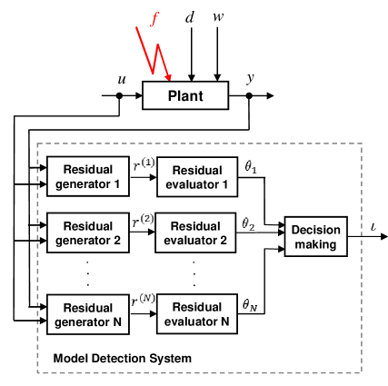
Figure 2: Basic model detection setup.

A typical model detection setting is shown in Fig. 2. A bank of $N$ residual generation filters (or residual generators) is used, with $r^{(i)}(t)$ being the output of the $i$-th residual generator. The $i$-th component $\theta_{i}$ of the $N$-dimensional evaluation vector $\theta$ usually represents an approximation of $\|r^{(i)}\|_{2}$, the $\mathcal{L}_{2}$- or $\ell_{2}$-norm of $r^{(i)}$. The $i$-th component of the $N$-dimensional decision vector $\iota$ is set to 0 if $\theta_{i}\leq\tau_{i}$ and 1 otherwise, where $\tau_{i}$ is a suitable threshold. The $j$-th model is “detected” if $\iota_{j}=0$ and $\iota_{i}=1$ for all $i\not=j$. It follows that model detection can be interpreted as a particular type of week fault isolation with $N$ signature vectors, where the $N$-dimensional $j$-th signature vector has all elements set to one, excepting the $j$-th entry which is set to zero. An alternative decision scheme can also be devised if $\theta_{i}$ can be associated with a distance function from the current model to the $i$-th model. In this case, $\iota$ is a scalar, set to $\iota=j$, where $j$ is the index for which $\theta_{j}=\min_{i=1:N}\theta_{i}$. Thus, the decision scheme selects that model $j$ which best fits with the current model characterized by the measured input and output data.

The underlying synthesis techniques of model detection systems rely on multiple-model descriptions of physical fault cases. Since different degrees of performance degradations can be easily described via multiple models, model detection techniques have potentially the capability to address certain fault identification aspects too.

3.2 Multiple Physical Fault Models

For physically modelled faults, each fault mode leads to a distinct model. Assume that we have $N$ LTI models describing the fault-free and faulty systems, and for $j=1,\ldots,N$ the $j$-th model is specified in the input-output form

$${\mathbf{y}}^{(j)}(\lambda)=G_{u}^{(j)}(\lambda){\mathbf{u}}(\lambda)+G_{d}^{(j)}(\lambda){\mathbf{d}}^{(j)}(\lambda)+G_{w}^{(j)}(\lambda){\mathbf{w}}^{(j)}(\lambda),$$ (35)

where $y^{(j)}(t)\in\mathds{R}^{p}$ is the output vector of the $i$-th system with control input $u(t)\in\mathds{R}^{m_{u}}$, disturbance input $d^{(j)}(t)\in\mathds{R}^{m_{d}^{(j)}}$ and noise input $w^{(j)}(t)\in\mathds{R}^{m_{w}^{(j)}}$, and where $G_{u}^{(j)}(\lambda)$, $G_{d}^{(j)}(\lambda)$ and $G_{w}^{(j)}(\lambda)$ are the TFMs from the corresponding plant inputs to outputs. The significance of disturbance and noise inputs, and the basic difference between them, have already been discussed in Section 2.2. The state-space realizations corresponding to the multiple model (35) are for $j=1,\ldots,N$ of the form

$$\begin{array}[]{rcl}E^{(j)}\lambda x^{(j)}(t)&=&A^{(j)}x^{(j)}(t)+B^{(j)}_{u}u(t)+B^{(j)}_{d}d^{(j)}(t)+B^{(j)}_{w}w^{(j)}(t)\,,\\ y^{(j)}(t)&=&C^{(j)}x^{(j)}(t)+D^{(j)}_{u}u(t)+D^{(j)}_{d}d^{(j)}(t)+D^{(j)}_{w}w^{(j)}(t)\,,\end{array}$$ (36)

where $x^{(j)}(t)\in\mathds{R}^{n^{(j)}}$ is the state vector of the $j$-th system and, generally, can have different dimensions for different systems.

The multiple-model description represents a very general way to describe plant models with various faults. For example, extreme variations of parameters representing the so-called parametric faults, can be easily described by multiple models.

3.3 Residual Generation

Assume we have $N$ LTI models of the form (35), for $j=1,...,N$, but the $N$ models originate from a common underlying system with $y(t)\in\mathds{R}^{p}$, the measurable output vector, and $u(t)\in\mathds{R}^{m_{u}}$, the known control input. Therefore, $y^{(j)}(t)\in\mathds{R}^{p}$ is the output vector of the $j$-th system with the control input $u(t)\in\mathds{R}^{m_{u}}$, disturbance input $d^{(j)}(t)\in\mathds{R}^{m_{d}^{(j)}}$ and noise input $w^{(j)}(t)\in\mathds{R}^{m_{w}^{(j)}}$, respectively, and $G_{u}^{(j)}(\lambda)$, $G_{d}^{(j)}(\lambda)$ and $G_{w}^{(j)}(\lambda)$ are the TFMs from the corresponding plant inputs to outputs. We explicitly assumed that all models are controlled with the same control inputs $u(t)$, but the disturbance and noise inputs $d^{(j)}(t)$ and $w^{(j)}(t)$, respectively, may differ for each component model. For complete generality of our problem formulations, we will allow that these TFMs are general rational matrices (proper or improper) for which we will not a priori assume any further properties.

Residual generation for model detection is performed using $N$ linear residual generators, which process the measurable system outputs $y(t)$ and known control inputs $u(t)$ and generate $N$ residual signals $r^{(i)}(t)$, $i=1,\ldots,N$, which serve for decision making on which model best matches the current input-output measurement data. As already mentioned, model detection can be interpreted as a week fault isolation problem with an $N\times N$ structure matrix $S$ having all its elements equal to one, excepting those on its diagonal which are zero. The task of model detection is thus to find out the model which best matches the measurements of outputs and inputs, by comparing the resulting decision vector $\iota$ with the set of signatures associated to each model and coded in the columns of $S$. The $N$ residual generation filters in their implementation form are described for $i=1,\ldots,N$, by the input-output relations

$${\mathbf{r}}^{(i)}(\lambda)=Q^{(i)}(\lambda)\left[\begin{array}[]{c}{\mathbf{y}}(\lambda)\\ {\mathbf{u}}(\lambda)\end{array}\right]\,,$$ (37)

where $y$ and $u$ is the actual measured system output and control input, respectively. The TFMs $Q^{(i)}(\lambda)$, for $i=1,\ldots,N$, must be proper and stable. The dimension $q_{i}$ of the residual vector component $r^{(i)}(t)$ can be chosen always one, but occasionally values $q_{i}>1$ may provide better sensitivity to model mismatches.

Assuming $y(t)=y^{(j)}(t)$, the residual signal component $r^{(i)}(t)$ in (37) generally depends on all system inputs $u(t)$, $d^{(j)}(t)$ and $w^{(j)}(t)$ via the system output $y^{(j)}(t)$. The internal form of the $i$-th filter driven by the $j$-th model is obtained by replacing in (37) ${\mathbf{y}}(\lambda)$ with ${\mathbf{y}}^{(j)}(\lambda)$ from (35). To make explicit the dependence of $r^{(i)}$ on the $j$-th model, we will use $\widetilde{r}^{(i,j)}$, to denote the $i$-th residual output for the $j$-th model. After replacing in (37) ${\mathbf{y}}(\lambda)$ with ${\mathbf{y}}^{(j)}(\lambda)$ from (35), we obtain

$$\begin{array}[]{lrl}{\widetilde{\mathbf{r}}}^{(i,j)}(\lambda)&:=&R^{(i,j)}(\lambda)\left[\begin{array}[]{c}{\mathbf{u}}(\lambda)\\ {\mathbf{d}}^{(j)}(\lambda)\\ {\mathbf{w}}^{(j)}(\lambda)\end{array}\right]\\ \\[-5.69054pt] &=&R_{u}^{(i,j)}(\lambda){\mathbf{u}}(\lambda)+R_{d}^{(i,j)}(\lambda){\mathbf{d}}^{(j)}(\lambda)+R_{w}^{(i,j)}(\lambda){\mathbf{w}}^{(j)}(\lambda)\,,\end{array}$$ (38)

with $R^{(i,j)}(\lambda):=\left[\begin{array}[]{c|c|c}R_{u}^{(i,j)}(\lambda)&R_{d}^{(i,j)}(\lambda)&R_{w}^{(i,j)}(\lambda)\end{array}\right]$ defined as

$$\left[\begin{array}[]{c|c|c}R_{u}^{(i,j)}(\lambda)&R_{d}^{(i,j)}(\lambda)&R_{w}^{(i,j)}(\lambda)\end{array}\right]:=Q^{(i)}(\lambda)\left[\begin{array}[]{c|c|c}G_{u}^{(j)}(\lambda)&G_{d}^{(j)}(\lambda)&G_{w}^{(j)}(\lambda)\\ I_{m_{u}}&0&0\end{array}\right]\,.$$ (39)

For a successfully designed set of filters $Q^{(i)}(\lambda)$, $i=1,\ldots,N$, the corresponding internal representations $R^{(i,j)}(\lambda)$ in (38) are also a proper and stable.

3.4 Model Detectability

The concept of model detectability concerns with the sensitivity of the components of the residual vector to individual models from a given collection of models. Assume that we have $N$ models, with the $j$-th model specified in the input-output form (35). For the discussion of the model detectability concept we will assume that no noise inputs are present in the models (35) (i.e., $w^{(j)}\equiv 0$ for $j=1,\ldots,N$). For model detection purposes, $N$ filters of the form (37) are employed. It follows from (38) that the $i$-th component $r^{(i)}$ of the residual $r$ is sensitive to the $j$-th model provided

$$R^{(i,j)}(\lambda):=\left[\begin{array}[]{cc}R_{u}^{(i,j)}(\lambda)&R_{d}^{(i,j)}(\lambda)\end{array}\right]\not=0\,.$$ (40)

This condition involves the use of both control and disturbance inputs for model detection and can be useful even in the case of absence of control inputs.

For most of practical applications, it is however necessary to be able to perform model detection also in the (unlikely) case when the disturbance inputs are zero. Therefore, to achieve model detection independently of the presence or absence of disturbances, it is meaningful to impose instead (40), the stronger condition

$$R_{u}^{(i,j)}(\lambda)\not=0\,.$$ (41)

This condition involves the use of only control inputs for model detection purposes and is especially relevant to active methods for model detection based on employing special inputs to help the discrimination between models.

Depending on which of the condition (40) or (41) are relevant for a particular model detection application, we define the following two concepts of model detectability.

Definition 6.

The multiple model defined by the $N$ component systems (35) with $w^{(j)}\equiv 0$ for $j=1,\ldots,N$, is extended model detectable if there exist $N$ filters of the form (37), such that $R^{(i,j)}(\lambda)$ defined in (40) fulfills $R^{(i,i)}(\lambda)=0$ for $i=1,\ldots,N$ and $R^{(i,j)}(\lambda)\not=0$ for all $i,j=1,\ldots,N$ such that $i\not=j$.

Definition 7.

The multiple model defined by the $N$ component systems (35) with $w^{(j)}\equiv 0$ for $j=1,\ldots,N$, is model detectable if there exist $N$ filters of the form (37), such that $R^{(i,j)}(\lambda)$ defined in (40) fulfills $R^{(i,i)}(\lambda)=0$ for $i=1,\ldots,N$ and $R_{u}^{(i,j)}(\lambda)\not=0$ for all $i,j=1,\ldots,N$ such that $i\not=j$.

The Definition 7 of model detectability involves the usage of only the control inputs for model detection purpose, and therefore implies the more general property of extended model detectability in Defintion 6. In the case of lack of disturbance inputs, the two definitions coincide.

The following result, proven in [16], characterizes the extended model detectability property.

Theorem 15.

The multiple model defined by the $N$ component systems (35) with $w^{(j)}\equiv 0$ for $j=1,\ldots,N$, is extended model detectable if and only if for $i=1,\ldots,N$

$$\mathop{\mathrm{rank}}\,[\,G_{d}^{(i)}(\lambda)\;\;G_{d}^{(j)}(\lambda)\;\;G_{u}^{(i)}(\lambda)\!-\!G_{u}^{(j)}(\lambda)\,]>\mathop{\mathrm{rank}}\,G_{d}^{(i)}(\lambda)\;\;\forall j\not=i\,.$$ (42)

The characterization of model detectability (using only control inputs) can be simply established as a corollary of this theorem.

Theorem 16.

The multiple model defined by the $N$ component systems (35) with $w^{(j)}\equiv 0$ for $j=1,\ldots,N$, is model detectable if and only if for $i=1,\ldots,N$

$$\mathop{\mathrm{rank}}\,[\,G_{d}^{(i)}(\lambda)\;\;G_{u}^{(i)}(\lambda)\!-\!G_{u}^{(j)}(\lambda)\,]>\mathop{\mathrm{rank}}\,G_{d}^{(i)}(\lambda)\;\;\forall j\not=i\,.$$ (43)

We can also define the concepts of strong model detectability and strong extended model detectability with respect to classes of persistent control inputs characterized by a set of complex frequencies $\Omega\subset\partial\mathds{C}_{s}$. The following definitions formalize the aim that for each model $j$, there exists at least one excitation signal class characterized by a frequency $\lambda_{z}\in\Omega$ for which all residual components $r^{(i)}(t)$ for $i\neq j$ are asymptotically nonzero and $r^{(j)}(t)$ asymptotically vanishes.

Definition 8.

The multiple model defined by the $N$ component systems (35) with $w^{(j)}\equiv 0$ for $j=1,\ldots,N$, is strong model detectable with respect to a set of frequencies $\Omega\subset\partial\mathds{C}_{s}$ if there exist $N$ stable filters of the form (37), such that $R^{(i,j)}(\lambda)$ defined in (40) fulfills $R^{(i,i)}(\lambda)=0$ for $i=1,\ldots,N$ and for all $i,j=1,\ldots,N$ with $i\not=j$, $\exists$ $\lambda_{z}\in\Omega$ such that $R_{u}^{(i,j)}(\lambda_{z})\not=0$.

Definition 9.

The multiple model defined by the $N$ component systems (35) with $w^{(j)}\equiv 0$ for $j=1,\ldots,N$, is strong extended model detectable with respect to a set of frequencies $\Omega\subset\partial\mathds{C}_{s}$ if there exist $N$ stable filters of the form (37), such that $R^{(i,j)}(\lambda)$ defined in (40) fulfills $R^{(i,i)}(\lambda)=0$ for $i=1,\ldots,N$ and for all $i,j=1,\ldots,N$ with $i\not=j$, $\exists$ $\lambda_{z}\in\Omega$ such that $R^{(i,j)}(\lambda_{z})\not=0$.

The following results characterize the strong model detectability property and, respectively, the strong extended model detectability property.

Theorem 17.

Let $\Omega\subset\partial\mathds{C}_{s}$ be a given set of frequencies, such that none of $\lambda_{z}\in\Omega$ is a pole of any of the component system (35), for $j=1,\ldots,N$. Then, the multiple model (35) with $w^{(j)}\equiv 0$ for $j=1,\ldots,N$, is strong model detectable with respect to $\Omega$ if and only if for $i=1,\ldots,N$

$$\forall j\not=i,\exists\lambda_{z}\in\Omega\text{ such that }\mathop{\mathrm{rank}}\,[\,G_{d}^{(i)}(\lambda_{z})\;\;G_{u}^{(i)}(\lambda_{z})\!-\!G_{u}^{(j)}(\lambda_{z})\,]>\mathop{\mathrm{rank}}\,G_{d}^{(i)}(\lambda_{z})\,.$$ (44)

Theorem 18.

Let $\Omega\subset\partial\mathds{C}_{s}$ be a given set of frequencies, such that none of $\lambda_{z}\in\Omega$ is a pole of any of the component system (35), for $j=1,\ldots,N$. Then, the multiple model (35) with $w^{(j)}\equiv 0$ for $j=1,\ldots,N$, is strong model detectable with respect to $\Omega$ if and only if for $i=1,\ldots,N$

$$\forall j\not=i,\exists\lambda_{z}\in\Omega\text{ such that }\mathop{\mathrm{rank}}\,\big{[}\,G_{d}^{(i)}(\lambda_{z})\;\;G_{d}^{(j)}(\lambda_{z})\;\;G_{u}^{(i)}(\lambda_{z})\!-\!G_{u}^{(j)}(\lambda_{z})\,\big{]}>\mathop{\mathrm{rank}}\,G_{d}^{(i)}(\lambda_{z})\,.$$ (45)

3.5 Model Detection Problems

In this section we formulate the exact and approximate synthesis problems of model detection filters for the collection of $N$ LTI systems (35). As in the case of the EFDIP or AFDIP, we seek $N$ linear residual generators (or model detection filters) of the form (37), which process the measurable system outputs $y(t)$ and known control inputs $u(t)$ and generate the $N$ residual signals $r^{(i)}(t)$ for $i=1,\ldots,N$. These signals serve for decision-making by comparing the pattern of fired and not fired residuals with the signatures coded in the columns of the associated standard $N\times N$ structure matrix $S$ with zeros on the diagonal and ones elsewhere. The standard requirements for the TFMs of the filters $Q^{(i)}(\lambda)$ in (37) are properness and stability. For practical purposes, the orders of the filter $Q^{(i)}(\lambda)$ must be as small as possible. Least order filters $Q^{(i)}(\lambda)$ can be usually achieved by employing scalar output least order filters.

In analogy to the formulations of the EFDIP and AFDIP, we use the internal form of the $i$-th residual generator (38) to formulate the basic model detection requirements. Independently of the presence of the noise inputs $w^{(j)}$, we will target that the $i$-th residual is exactly decoupled from the $i$-th model if $w^{(i)}\equiv 0$ and is sensitive to the $j$-th model, for all $j\not=i$. These requirements can be easily translated into algebraic conditions using the internal form (38) of the $i$-th residual generator. If both control and disturbance inputs are involved in the model detection then the following conditions have to be fulfilled

$$\begin{array}[]{ll}(i)&[\,R_{u}^{(i,i)}(\lambda)\;\;R_{d}^{(i,i)}(\lambda)\,]=0,\;\;i=1,\ldots,N\,,\\ (ii)&[\,R_{u}^{(i,j)}(\lambda)\;\;R_{d}^{(i,j)}(\lambda)\,]\not=0,\;\;\forall j\not=i,\text{ with }[\,R_{u}^{(i,j)}(\lambda)\;\;R_{d}^{(i,j)}(\lambda)\,]\text{ stable.}\end{array}$$ (46)

while if only control inputs have to be employed for model detection, then the following conditions have to be fulfilled

$$\begin{array}[]{ll}(i)&[\,R_{u}^{(i,i)}(\lambda)\;\;R_{d}^{(i,i)}(\lambda)\,]=0,\;\;i=1,\ldots,N\,,\\ (ii)^{\prime}&R_{u}^{(i,j)}(\lambda)\not=0,\;\;\forall j\not=i,\text{ with }[\,R_{u}^{(i,j)}(\lambda)\;\;R_{d}^{(i,j)}(\lambda)\,]\text{ stable.}\end{array}$$ (47)

Here, $(i)$ is the model decoupling condition for the $i$-th model in the $i$-th residual component, while $(ii)$ and $(ii)^{\prime}$ are the model sensitivity condition of the $i$-th residual component to all models, excepting the $i$-th model. In the case when condition $(i)$ cannot be fulfilled (e.g., due to lack of sufficient measurements), some (or even all) components of $d^{(i)}(t)$ can be redefined as noise inputs and included in $w^{(i)}(t)$.

In what follows, we formulate the exact and approximate model detection problems, for which we give the existence conditions of the solutions. For the proof of the results consult [16].

3.5.1 EMDP – Exact Model Detection Problem

The standard requirement for solving the exact model detection problem (EMDP) is to determine for the multiple model (35), in the absence of noise input (i.e., $w^{(j)}\equiv 0$ for $j=1,\ldots,N$), a set of $N$ proper and stable filters $Q^{(i)}(\lambda)$ such that, for $i=1,\ldots,N$, the conditions (46) or (47) are fulfilled. These conditions are similar to the model detectability requirement and lead to the following solvability condition:

Theorem 19.

For the multiple model (35) with $w^{(j)}\equiv 0$ for $j=1,\ldots,N$, the EMDP is solvable with conditions (46) if and only if the multiple model (35) is extended model detectable.

Theorem 20.

For the multiple model (35) with $w^{(j)}\equiv 0$ for $j=1,\ldots,N$, the EMDP is solvable with conditions (47) if and only if the multiple model (35) is model detectable.

Let $\Omega\subset\partial\mathds{C}_{s}$ be a given set of frequencies which characterize the relevant persistent input and disturbance signals. We can give a similar result in the case when the EMDP is solved, by replacing the condition $(ii)^{\prime}$ in (47), with the strong model detection condition:

$$(ii)^{\prime\prime}\;\;\forall j\not=i,\;\;\exists\lambda_{z}\in\Omega\text{ such that }R_{u}^{(i,j)}(\lambda_{z})\not=0,\;\;\text{ with }[\,R_{u}^{(i,j)}(\lambda)\;\;R_{d}^{(i,j)}(\lambda)\,]\text{ stable.}$$ (48)

The solvability condition of the EMDP with the strong model detection condition above is precisely the strong model detectability requirement as stated by the following theorem.

Theorem 21.

Let $\Omega$ be the set of frequencies which characterize the persistent control input signals. For the multiple model (35) with $w^{(j)}\equiv 0$ for $j=1,\ldots,N$, the EMDP with the strong model detectability condition (48) is solvable if and only if the multiple model (35) is strong model detectable.

A similar result holds when targeting the strong extended model detectability property.

3.5.2 AMMP – Approximate Model Detection Problem

The effects of the noise input $w^{(i)}(t)$ can usually not be fully decoupled from the residual $r^{(i)}(t)$. In this case, the basic requirements for the choice of $Q^{(i)}(\lambda)$ can be expressed as achieving that the residual $r^{(i)}(t)$ is influenced by all models in the multiple model (35), while the influence of the $i$-th model is only due to the noise signal $w^{(i)}(t)$ and is negligible. Using the internal form (38) of the $i$-th residual generator, for the approximate model detection problem (AMDP) the following additional conditions to (46) or (47) have to be fulfilled:

$$\begin{array}[]{ll}(iii)&R_{w}^{(i,i)}(\lambda)\approx 0,\;\;\textrm{with}\;\;R_{w}^{(i,i)}(\lambda)\;\;\textrm{stable;}\\ (iv)&R_{w}^{(i,j)}(\lambda)\;\;\textrm{stable}\;\forall j\not=i.\end{array}$$ (49)

Here, $(iii)$ is the attenuation condition of the noise input.

The solvability conditions of the AMDP are precisely those of the EMDP:

Theorem 22.

For the multiple model (35) the AMDP is solvable if and only the EMDP is solvable.

3.6 Analysis and Performance Evaluation of Model Detection Filters

3.6.1 Distances between Models

For the setup of model detection applications, an important first step is the selection of a representative set of component models to serve for the design of model detection filter. A practical requirement to set up multiple models as in (35) or (36) is to choose a set of component models, such that, each component model is sufficiently far away of the rest of models. A suitable tool to measure the distance between two models is the $\nu$-gap metric introduced in [18]. For two transfer function matrices $G_{1}(\lambda)$ and $G_{2}(\lambda)$ of the same dimensions, consider the normalized left coprime factorization $G_{1}(\lambda)=\widetilde{M}_{1}^{-1}(\lambda)\widetilde{N}_{1}(\lambda)$ (i.e., $\big{[}\,\widetilde{N}_{1}(\lambda)\;\widetilde{M}_{1}(\lambda)\,\big{]}$ is coinner) and the normalized right coprime factorizations $G_{1}(\lambda)=N_{1}(\lambda)M_{1}^{-1}(\lambda)$ and $G_{2}(\lambda)=N_{2}(\lambda)M_{2}^{-1}(\lambda)$ (i.e., $\left[\begin{smallmatrix}N_{i}(\lambda)\\ M_{1}(\lambda)\end{smallmatrix}\right]$ is inner for $i=1,2$). With $\widetilde{L}_{2}(\lambda):=[\,-\widetilde{M}_{2}(\lambda)\;\widetilde{N}_{2}(\lambda)\,]$, $R_{i}(\lambda):=\left[\begin{smallmatrix}N_{i}(\lambda)\\ M_{i}(\lambda)\end{smallmatrix}\right]$ for $i=1,2$, and $g(\lambda):=\det\big{(}R_{2}^{\sim}(\lambda)R_{1}(\lambda)\big{)}$, we have the following definition of the $\nu$-gap metric between the two transfer-function matrices:

$$\delta_{\nu}(G_{1}(\lambda),G_{2}(\lambda)):=\left\{\begin{array}[]{cl}\big{\|}\widetilde{L}_{2}(\lambda)R_{1}(\lambda)\big{\|}_{\infty}&\text{if }g(\lambda)\neq 0\;\forall\lambda\in\partial\mathds{C}_{s}\text{ and }\mathop{\mathrm{wno}}(g)=0,\\ 1&\text{otherwise},\end{array}\right.$$ (50)

where $\mathop{\mathrm{wno}}(g)$ denotes the winding number of $g(\lambda)$ about the appropriate critical point for $\lambda$ following the corresponding standard Nyquist contour. The winding number of $g(\lambda)$ can be determined as the difference between the number of unstable zeros of $g(\lambda)$ and the number of unstable poles of $g(\lambda)$ [17]. Generally, for any $G_{1}(\lambda)$ and $G_{2}(\lambda)$, we have $0\leq\delta_{\nu}(G_{1}(\lambda),G_{2}(\lambda))\leq 1$. If $\delta_{\nu}\big{(}G_{1}(\lambda),G_{2}(\lambda)\big{)}$ is small, then we can say that $G_{1}(\lambda)$ and $G_{2}(\lambda)$ are close and it is likely that a model detection filter suited for $G_{1}(\lambda)$ will also work with $G_{2}(\lambda)$, and therefore, one of the two models can be probably removed from the set of component models. On the other side, if $\delta_{\nu}\big{(}G_{1}(\lambda),G_{2}(\lambda)\big{)}$ is nearly equal to 1, then $G_{1}(\lambda)$ and $G_{2}(\lambda)$ are sufficiently distinct, such that an easy discrimination between the two models is possible. A common criticism of the $\nu$-gap metric is that there are many transfer function matrices $G_{2}(\lambda)$ at a distance $\delta_{\nu}\big{(}G_{1}(\lambda),G_{2}(\lambda)\big{)}=1$ to a given $G_{1}(\lambda)$, but the metric fails to differentiate between them. However, this aspect should not rise difficulties in model detection applications.

In [19], the point-wise $\nu$-gap metric is also defined to evaluate the distance between two models in a single frequency point. If $\lambda_{k}$ is a fixed complex frequency, then the point-wise $\nu$-gap metric between two transfer-function matrices $G_{1}(\lambda)$ and $G_{2}(\lambda)$ at the frequency $\lambda_{k}$ is:

$$\delta_{\nu}(G_{1}(\lambda_{k}),G_{2}(\lambda_{k})):=\left\{\begin{array}[]{cl}\big{\|}\widetilde{L}_{2}(\lambda_{k})R_{1}(\lambda_{k})\big{\|}_{2}&\text{if }g(\lambda)\neq 0\;\forall\lambda\in\partial\mathds{C}_{s}\text{ and }\mathop{\mathrm{wno}}(g)=0,\\ 1&\text{otherwise},\end{array}\right.$$ (51)

For a set of $N$ component models with input-output forms as in (35), it is useful to determine the pairwise $\nu$-gap distances between the control input channels of the component models by defining the symmetric matrix $\Delta$, whose $(i,j)$-th entry is the $\nu$-gap distance between the transfer-function matrices of the $i$-th and $j$-th model

$$\Delta_{ij}:=\delta_{\nu}\big{(}G_{u}^{(i)}(\lambda),G_{u}^{(j)}(\lambda)\big{)}.$$ (52)

It follows that $\Delta$ has all its diagonal elements zero. For model detection applications all off-diagonal elements of $\Delta$ must be nonzero, otherwise there are models which can not be potentially discriminated. The definition (52) of the distances between the $i$-th and $j$-th models focuses only on the control input channels. In most of practical applications of the model detection, this is perfectly justified by the fact that, a certain control activity is always necessary, to ensure reliable discrimination among models, independently of the presence or absence of disturbances. However, if the disturbance inputs are relevant to perform model detection (e.g., there are no control inputs), and all component models share the same disturbance inputs (i.e., $d^{(j)}(t)=d(t)$ for $j=1,\ldots,N$), then the definition of $\Delta$ in (52) can be modified to include the disturbance inputs as well

$$\Delta_{ij}:=\delta_{\nu}\big{(}\big{[}\,G_{u}^{(i)}(\lambda)\;G_{d}^{(i)}(\lambda)\,\big{]},\big{[}\,G_{u}^{(j)}(\lambda)\;G_{d}^{(j)}(\lambda)\,\big{]}\big{)}.$$ (53)

If $\lambda_{k}$, $k=1,\ldots,n_{f}$, is a set of $n_{f}$ frequency values, then, instead (52), we can use the maximum of the point-wise distances

$$\Delta_{ij}:=\max_{k}\delta_{\nu}\big{(}G_{u}^{(i)}(\lambda_{k}),G_{u}^{(j)}(\lambda_{k})\big{)},$$

and similarly, instead (53), we can use the maximum of the point-wise distances

$$\Delta_{ij}:=\max_{k}\delta_{\nu}\big{(}\big{[}\,G_{u}^{(i)}(\lambda_{k})\;G_{d}^{(i)}(\lambda_{k})\,\big{]},\big{[}\,G_{u}^{(j)}(\lambda_{k})\;G_{d}^{(j)}(\lambda_{k})\,\big{]}\big{)}.$$

Besides the $\nu$-gap distance between two transfer function matrices, it is possible to use distances defined in terms of the $\mathcal{H}_{\infty}$ norm or the $\mathcal{H}_{2}$ norm of the difference between them. Thus we can use instead (52)

$$\Delta_{ij}:=\big{\|}G_{u}^{(i)}(\lambda)-G_{u}^{(j)}(\lambda)\big{\|}_{\infty}$$

or

$$\Delta_{ij}:=\big{\|}G_{u}^{(i)}(\lambda)-G_{u}^{(j)}(\lambda)\big{\|}_{2}.$$

If $\lambda_{k}$, $k=1,\ldots,n_{f}$, is a set of $n_{f}$ frequency values, then, instead of the above norm-based distances, we can use the maximum of the point-wise distances

$$\Delta_{ij}:=\max_{k}\big{\|}G_{u}^{(i)}(\lambda_{k})-G_{u}^{(j)}(\lambda_{k})\big{\|}_{2}.$$

3.6.2 Distances to a Current Model

An important aspect which arises in model detection applications, where the use of $\nu$-gap metric could be instrumental, is to assess the nearness of a current model, with the input-output form

$${\mathbf{y}}(\lambda)=\widetilde{G}_{u}(\lambda){\mathbf{u}}(\lambda)+\widetilde{G}_{d}(\lambda){\mathbf{d}}(\lambda)+\widetilde{G}_{w}(\lambda){\mathbf{w}}(\lambda),$$ (54)

to the component models in (35). This involves evaluating, for $j=1,\ldots,N$, the distances between the control input channels of the models (35) and (54) as

$$\eta_{j}:=\delta_{\nu}\big{(}G_{u}^{(j)}(\lambda),\widetilde{G}_{u}(\lambda)\big{)}.$$ (55)

It is also of interest to determine the index $\ell$ of that component model for which $\eta_{\ell}$ is the least distance. This allows to assign the model (54) to the (open) set of nearby models to the $\ell$-th component model and can serve for checking the preservation of this property by the mapping achieved by the model detection filters via the norms of internal forms $R_{u}^{(i,j)}(\lambda)$ in (38).

If the disturbance inputs are also relevant to the model detection application, then a similar extension as above is possible to assess the distances between a current model and a set of component models by redefining $\eta_{j}$ in (55) as

$$\eta_{j}:=\delta_{\nu}\big{(}\big{[}\,G_{u}^{(j)}(\lambda)\;G_{d}^{(j)}(\lambda)\,\big{]},\big{[}\,\widetilde{G}_{u}(\lambda)\;\widetilde{G}_{d}(\lambda)\,\big{]}\big{)}.$$ (56)

As before, we can alternatively use distances defined in terms of the $\mathcal{H}_{\infty}$ norm or the $\mathcal{H}_{2}$ norm. Thus, instead (55), we can use

$$\eta_{j}:=\big{\|}G_{u}^{(j)}(\lambda)-\widetilde{G}_{u}(\lambda)\big{\|}_{\infty}$$

or

$$\eta_{j}:=\big{\|}G_{u}^{(j)}(\lambda)-\widetilde{G}_{u}(\lambda)\big{\|}_{2}.$$

If $\lambda_{k}$, $k=1,\ldots,n_{f}$, is a given set of $n_{f}$ frequency values, then, instead of the above peak distances, we can use the maximum of the point-wise distances over the finite set of frequency values.

3.6.3 Distance Mapping Performance

One of the goals of the model detection is to achieve a special mapping of the distances between component models using $N$ model detection filters of the form (37) such that the norms of the transfer-function matrices $R_{u}^{(i,j)}(\lambda)$ or of $\big{[}\,R_{u}^{(i,j)}(\lambda)\;R_{d}^{(i,j)}(\lambda)\,\big{]}$ in the internal forms of the filters (38) qualitatively reproduce the $\nu$-gap distances expressed by the $\Delta$ matrix, whose $(i,j)$-th entries are defined in (52) or (53, respectively. The preservation of this distance mapping property is highly desirable, and the choice of model detection filters must be able to ensure this feature (at least partially for the nearest models). For example, the choice of the $i$-th filter $Q^{(i)}(\lambda)$ as a left annihilator of $\left[\begin{smallmatrix}G_{u}^{(i)}(\lambda)&G_{d}^{(i)}(\lambda)\\ I_{m_{u}}&0\end{smallmatrix}\right]$ ensures (see [16, Remark 6.1]) that norm of $\big{[}\,R_{u}^{(i,j)}(\lambda)\;R_{u}^{(i,j)}(\lambda)\,\big{]}$ can be interpreted as a weighted distance between the $i$-th and $j$-th component models. It follows that the distance mapping performance of a set of model detection filters $Q^{(i)}(\lambda)$, $i=1,\ldots,N$ can be assessed by computing mapped distance matrix $\Gamma$, whose $(i,j)$-th entry is

$$\Gamma_{ij}=\big{\|}R_{u}^{(i,j)}(\lambda)\big{\|}_{\infty}$$ (57)

or, if the disturbance inputs are relevant,

$$\Gamma_{ij}=\big{\|}\big{[}\,R_{u}^{(i,j)}(\lambda)\;R_{d}^{(i,j)}(\lambda)\,\big{]}\big{\|}_{\infty}.$$ (58)

Using the above choice of the filter $Q^{(i)}(\lambda)$, we have that all diagonal elements of $\Gamma$ are zero. Additionally, to guarantee model detectability or extended model detectability (see Section 3.4), any valid design of the model detection filters must guarantee that all off-diagonal elements of $\Gamma$ are nonzero. These two properties of $\Gamma$ allows to unequivocally identify the exact matching of the current model with one (and only one) of the $N$ component models.

Two other properties of $\Gamma$ are desirable, when solving model detection applications. The first property is the symmetry of $\Gamma$. In contrast to $\Delta$, $\Gamma$ is generally not symmetric, excepting for some particular classes of component models and for special choices of model detection filters. For example, this property can be ensured if all component models are stable and have no disturbance inputs, by choosing $Q^{(i)}(\lambda)=\big{[}\,I\;-G_{u}^{(i)}(\lambda)\,\big{]}$, in which case $R_{u}^{(i,j)}(\lambda)=-R_{u}^{(j,i)}(\lambda)$. Ensuring the symmetry of $\Gamma$, although very desirable, is in general difficult to be achieved. In practice, it is often sufficient to ensure via suitable scaling that the gains of first row and first column are equal.

The second desirable property of the mapping $\Delta_{ij}\rightarrow\Gamma_{ij}$ is the monotonic mapping property of distances, which is the requirement that for all $i$ and $k$ ($i,k=1,\ldots,N$), if $\Delta_{ij}<\Delta_{ik}$, then $\Gamma_{ij}<\Gamma_{ik}$. Ensuring this property, make easier to address model identification problems for which no exact matching between the current model and any one of the component models can be assumed.

If $\lambda_{k}$, $k=1,\ldots,n_{f}$, is a given set of $n_{f}$ frequency values, then, instead of the peak distances in (57) or in (58), we can use the maximum of the point-wise distances over the finite set of frequency values, to assess the strong model detectability or the extended strong model detectability, respectively (see Section 3.4).

3.6.4 Distance Matching Performance

To evaluate the distance matching property of the model detection filters in the case when no exact matching between the current model (54) and any one of the component models (35) can be assumed, we can define the corresponding current internal forms as

$$\left[\begin{array}[]{c|c|c}\widetilde{R}_{u}^{(i)}(\lambda)&\widetilde{R}_{d}^{(i)}(\lambda)&\widetilde{R}_{w}^{(i)}(\lambda)\end{array}\right]:=Q^{(i)}(\lambda)\left[\begin{array}[]{c|c|c}\widetilde{G}_{u}(\lambda)&\widetilde{G}_{d}(\lambda)&\widetilde{G}_{w}(\lambda)\\ I_{m_{u}}&0&0\end{array}\right]$$ (59)

and evaluate the mapped distances $\gamma_{i}$, for $i=1,\ldots,N$, defined as

$$\gamma_{i}:=\big{\|}\widetilde{R}_{u}^{(i)}(\lambda)\big{\|}_{\infty}$$ (60)

or, if the disturbance inputs are relevant,

$$\gamma_{i}:=\big{\|}\big{[}\,\widetilde{R}_{u}^{(i)}(\lambda)\;\widetilde{R}_{d}^{(i)}(\lambda)\,\big{]}\big{\|}_{\infty}.$$ (61)

The index $\ell$ of the smallest value $\gamma_{\ell}$ provides (for a well designed set of model detection filters) the index of the best matching component model of the current model.

If $\lambda_{k}$, $k=1,\ldots,n_{f}$, is a given set of $n_{f}$ frequency values, then, instead of the above peak distances, we can use the maximum of the point-wise distances over the finite set of frequency values.

3.6.5 Model Detection Noise Gaps

The noise attenuation performance of model detection filters can be characterized via the noise gaps achieved by individual filters. The noise gap for the $i$-th filter can be defined in terms of the resulting internal forms (38) as the ratio $\eta_{i}:=\beta_{i}/\gamma_{i}$, where

$$\beta_{i}:=\min_{j\neq i}\big{\|}R_{u}^{(i,j)}(\lambda)\big{\|}_{\infty}$$ (62)

and

$$\gamma_{i}:=\big{\|}R_{w}^{(i,i)}(\lambda)\big{\|}_{\infty}.$$ (63)

The values of $\beta_{i}>0$, for $i=1,\ldots,N$ characterize the model detectability property of the collection of the $N$ component models (35), while $\gamma_{i}$ characterizes the worst-case influence of noise inputs on the $i$-th residual component. If $\gamma_{i}=0$ (no noise), then $\eta_{i}=\infty$.

If the disturbance inputs are relevant for the model detection, then instead (62) we can use the following definition of $\beta_{i}$

$$\beta_{i}:=\min_{j\neq i}\big{\|}\big{[}\,R_{u}^{(i,j)}(\lambda)\;R_{d}^{(i,j)}(\lambda)\,\big{]}\big{\|}_{\infty}.$$ (64)

In this case, $\beta_{i}>0$, for $i=1,\ldots,N$ characterize the extended model detectability property of the collection of the $N$ component models (35).

If $\lambda_{k}$, $k=1,\ldots,n_{f}$, is a given set of $n_{f}$ frequency values, then, instead of (62) we use the maximum of the point-wise distances over the finite set of frequency values

$$\beta_{i}:=\min_{j\neq i}\max_{k}\big{\|}R_{u}^{(i,j)}(\lambda_{k})\big{\|}_{\infty}$$ (65)

and instead of (64) we use

$$\beta_{i}:=\min_{j\neq i}\max_{k}\big{\|}\big{[}\,R_{u}^{(i,j)}(\lambda_{k})\;R_{d}^{(i,j)}(\lambda_{k})\,\big{]}\big{\|}_{\infty}.$$ (66)

4 Description of FDITOOLS

This user’s guide is intended to provide users basic information on the FDITOOLS collection to solve the fault detection and isolation problems formulated in Section 2.6 and the model detection problem formulated in Section 3.5. The notations and terminology used throughout this guide have been introduced and extensively discussed in the accompanying book [16], which also represents the main reference for the implemented computational methods underlying the analysis and synthesis functions of FDITOOLS. Information on the requirements for installing FDITOOLS are given in Appendix A.

In this section, we present first a short overview of the existing functions of FDITOOLS and then, we illustrate a typical work flow by solving an EFDIP. In-depth information on the command syntax of the functions of the FDITOOLS collection is given is Sections 4.4 and 4.8. To execute the examples presented in this guide, simply paste the presented code sequences into the MATLAB command window. More involved examples are given in several case studies presented in [16].

4.1 Quick Reference Tables

The current release of FDITOOLS is version V1.0, dated November 30, 2018. The corresponding Contents.m file is listed in Appendix B. This section contains quick reference tables for the functions of the FDITOOLS collection. The M-files available in the current version of FDITOOLS, which are documented in this user’s guide, are listed below by category, with short descriptions.

Demonstration
FDIToolsdemo	Demonstration of Fault Detection and Isolation Tools
Setup of synthesis models
fdimodset	Setup of models for solving FDI synthesis problems.
mdmodset	Setup of models for solving model detection synthesis problems.
FDI Related Analysis
fdigenspec	Generation of achievable FDI specifications.
fdichkspec	Feasibility analysis of a set of FDI specifications.
Model Detection Related Analysis
mddist	Computation of distances between component models.
mddist2c	Computation of distances to a set of component models.

Performance evaluation of FDI filters
fditspec	Computation of the weak or strong structure matrix.
fdisspec	Computation of the strong structure matrix.
fdifscond	Fault sensitivity condition of FDI filters.
fdif2ngap	Fault-to-noise gap of FDI filters.
fdimmperf	Model-matching performance of FDI filters.
Performance evaluation of model detection filters
mdperf	Model detection distance mapping performance.
mdmatch	Model detection distance matching performance.
mdgap	Noise gaps of model detection filters.
Synthesis of fault detection filters
efdsyn	Exact synthesis of fault detection filters.
afdsyn	Approximate synthesis of fault detection filters.
efdisyn	Exact synthesis of fault detection and isolation filters.
afdisyn	Approximate synthesis of fault detection and isolation filters.
emmsyn	Exact model matching based synthesis of FDI filters.
ammsyn	Approximate model matching based synthesis of FDI filters.
Synthesis of model detection filters
emdsyn	Exact synthesis of model detection filters.
amdsyn	Approximate synthesis of model detection filters.

4.2 Getting Started

In this section we shortly illustrate the typical steps of solving a fault detection and isolation problem, starting with building an adequate fault model, performing preliminary analysis, selecting the suitable synthesis approach, and evaluating the computed results.

4.2.1 Building Models with Additive Faults

In-depth information on how to create and manipulate LTI system models and arrays of LTI system models are available in the online documentation of the Control System Toolbox and in its User’ Guide [2]. These types of models are the basis of the data objects used in the FDITOOLS collection.

The input plant models with additive faults used by all synthesis functions of the FDITOOLS collection are LTI models of the form (2), given via their equivalent descriptor system state-space realizations of the form (3). The object-oriented framework employed in the Control System Toolbox has been used to define the LTI plant models, by defining several input groups corresponding to various input signal. The employed standard definitions of input groups are: ’controls’ for the control inputs $u(t)$, ’disturbances’ for the disturbance inputs $d(t)$, ’faults’ for the fault inputs $f(t)$, and ’noise’ for the noise inputs $w(t)$. For convenience, occasionally an input group ’aux’ can be also defined for additional inputs. For different ways to define input groups, see the documentation of the Control System Toolbox [2].

Once you have a plant model for a system without faults, you can construct models with faults using simple commands in the Control System Toolbox or using the model setup function fdimodset. For example, consider a plant model sys with 3 inputs, 3 outputs and 3 state components. Assume that the first two inputs are control inputs which are susceptible to actuator faults and the third input is a disturbance input, which is not measurable and therefore is considered as an unknown input. All outputs are measurable, and assume that the first output is susceptible to sensor fault. The following commands generate a plant model with additive faults as described above:

rng(50); sys = rss(3,3,3);
inputs = struct(’c’,1:2,’d’,3,’f’,1:2,’fs’,1);
sysf = fdimodset(sys,inputs);

4.2.2 Determining the Achievable FDI Specifications

To determine the achievable strong FDI specifications with respect to constant faults, the function fdigenspec can be used as follows:

S = fdigenspec(sysf,struct(’FDFreq’,0));

For the above example, the possible fault signatures are contained in the generic structure matrix

$$S=\left[\begin{array}[]{ccc}0&1&1\\ 1&0&1\\ 1&1&0\\ 1&1&1\end{array}\right],$$

which indicates that the EFDP is solvable (last row of $S$) and the EFDIP is also solvable using the specifications contained in the rows of

$$S_{FDI}=\left[\begin{array}[]{ccc}0&1&1\\ 1&0&1\\ 1&1&0\end{array}\right].$$

4.2.3 Designing an FDI Filter Using efdisyn

To solve the EFDIP, an option structure is used to specify various user options for the synthesis function efdisyn. Frequently used options are the desired stability degree for the poles of the fault detection filter, the requirement for performing least order synthesis, or values for the tolerances used for rank computations or fault detectability tests. The user options can be specified by setting appropriately the respective fields in a MATLAB structure options. For example, the desired stability degree of $-2$ of the filter, the targeted fault signature specification $S_{FDI}$, and the frequency $0$ for strong synthesis (for constant faults), can be set using

options = struct(’sdeg’,-2,’SFDI’,S(1:3,:),’FDFreq’,0);

A solution of the EFDIP, for the selected structure matrix $S_{FDI}$, can be computed using the function efdisyn as given below

[Q,R,info] = efdisyn(sysf,options);

The resulting bank of scalar output fault detection filters, in implementation form, is contained in Q (stored as an one-dimensional cell array of systems), while the corresponding internal forms of the bank of filters are contained in the cell array R. The information structure info contains further information on the resulting designs.

4.2.4 Assessing the Residual Generator

For assessment purposes, often simulations performed using the resulting internal form provide sufficient qualitative information to verify the obtained results. The example below illustrates how to simulate step inputs from faults using the computed cell array R containing the internal form of the filter.

Rf = vertcat(R{:});  % build the global internal form of the filter
Rf.OutputName = strcat(strseq(’r_{’,1:3),’}’);
Rf.InputName  = strcat(strseq(’f_{’,1:3),’}’);
step(Rf,8);

A typical output of this computation can be used to assess the achieved fault signatures as shown in Fig. 3. As it can be observed, the diagonal entries of the overall transfer-function matrix of Rf are zero, while all off-diagonal entries are nonzero.

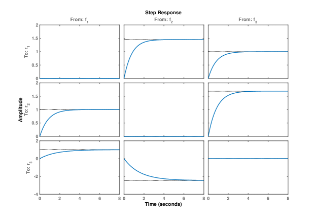
Figure 3: Step responses from the fault inputs.

The resulting strong structure matrix and the fault sensitivity conditions the resulting bank of internal filters can be obtained directly from the computed internal form R:

S_strong = fdisspec(R)
fscond   = fdifscond(R,0,S_strong)

The resulting values of the fault sensitivity conditions $\{0.6905,0.5918,0.4087\}$ indicate an acceptable sensitivity of all residual components to individual faults.

4.3 Functions for the Setup of Synthesis Models

The functions for the setup of synthesis models allow to easily define models in forms suitable for the use of analysis and synthesis functions.

4.3.1 fdimodset

Syntax

SYSF = fdimodset(SYS,INPUTS)

Description

fdimodset builds synthesis models with additive faults to be used in conjunction with the analysis and synthesis functions of FDI filters.

Input data

SYS is a LTI system in a descriptor system state-space form

$$E\lambda x(t) =Ax(t)+B\widetilde{u}(t),$$ (67)

$$y(t) =Cx(t)+D\widetilde{u}(t),$$

where $y(t)\in\mathds{R}^{p}$ is the system output and $\widetilde{u}(t)\in\mathds{R}^{m}$ is the system global input, which usually includes the control and disturbance inputs, but may also explicitly include fault inputs, noise inputs and auxiliary inputs.

INPUTS is a MATLAB structure used to specify the indices of the columns of the matrices $B$ and, respectively $D$, which correspond to the control, disturbance, fault, noise and auxiliary inputs, using the following fields:

INPUTS fields	Description
controls	vector of indices of the control inputs (Default: void)
c	alternative short form to specify the indices of the control inputs (Default: void)
disturbances	vector of indices of the disturbance inputs (Default: void)
d	alternative short form to specify the indices of the disturbance inputs (Default: void)
faults	vector of indices of the fault inputs (Default: void)
f	alternative short form to specify the indices of the fault inputs (Default: void)
faults_sen	vector of indices of the outputs subject to sensor faults (Default: void)
fs	alternative short form to specify the indices of the outputs subject to sensor faults (Default: void)
noise	vector of indices of the noise inputs (Default: void)
n	alternative short form to specify the indices of the noise inputs (Default: void)
aux	vector of indices of the auxiliary inputs (Default: void)

Output data

SYSF is a LTI system in the state-space form

$$E\lambda x(t) =Ax(t)+B_{u}u(t)+B_{d}d(t)+B_{f}f(t)+B_{w}w(t)+B_{v}v(t),$$ (68)

$$y(t) =Cx(t)+D_{u}u(t)+D_{d}d(t)+D_{f}f(t)+D_{w}w(t)+B_{v}v(t).$$

where $u(t)\in\mathds{R}^{m_{u}}$ are the control inputs, $d(t)\in\mathds{R}^{m_{d}}$ are the disturbance inputs, $f(t)\in\mathds{R}^{m_{f}}$ are the fault inputs, $w(t)\in\mathds{R}^{m_{w}}$ are the noise inputs and $v(t)\in\mathds{R}^{m_{v}}$ are auxiliary inputs. Any of the inputs components $u(t)$, $d(t)$, $f(t)$, $w(t)$ or $v(t)$ can be void. The input groups for $u(t)$, $d(t)$, $f(t)$, $w(t)$ and $v(t)$ have the standard names ’controls’, ’disturbances’, ’faults’, ’noise’ and ’aux’, respectively. The resulting model SYSF inherits the sampling time of the original model SYS.

Remark on input and output data

The function fdimodset can also be employed if SYS is an $N\times 1$ or $1\times N$ array of LTI models, in which case the resulting SYSF is also an $N\times 1$ or $1\times N$ array of LTI models, respectively.

Method

The system matrices $B_{u}$, $B_{d}$, $B_{f}$, $B_{w}$, $B_{v}$, and $D_{u}$, $D_{d}$, $D_{f}$, $D_{w}$, $D_{v}$ in the resulting model (68) are defined by specifying the indices of the columns of the matrices $B$ and, respectively $D$, in the model (67) which correspond to the control, disturbance, fault, noise and auxiliary inputs. If the system SYS in (67) has the equivalent input-output form

$${\mathbf{y}}(\lambda)=G(\lambda)\widetilde{\mathbf{u}}(\lambda)$$ (69)

and the resulting system SYSF in (68) has the equivalent input-output form

$${\mathbf{y}}(\lambda)=G_{u}(\lambda){\mathbf{u}}(\lambda)+G_{d}(\lambda){\mathbf{d}}(\lambda)+G_{f}(\lambda){\mathbf{f}}(\lambda)+G_{w}(\lambda){\mathbf{w}}(\lambda)+G_{v}(\lambda){\mathbf{v}}(\lambda),$$ (70)

then the following relations exist among the above transfer function matrices

$$\begin{array}[]{lcl}G_{u}(\lambda)&=&G(\lambda)S_{u},\\ G_{d}(\lambda)&=&G(\lambda)S_{d},\\ G_{f}(\lambda)&=&[\,G(\lambda)S_{f}\;S_{s}\,],\\ G_{w}(\lambda)&=&G(\lambda)S_{w},\\ G_{v}(\lambda)&=&G(\lambda)S_{v},\end{array}$$

where $S_{u}$, $S_{d}$, $S_{f}$, $S_{w}$, and $S_{v}$ are columns of the identity matrix $I_{m}$ and $S_{s}$ is formed from the columns of the indentity matrix $I_{p}$. These (selection) matrices are used to select the corresponding columns of $G(\lambda)$, and thus to obtain the input and feedthrough matrices of the model (68) from those of the model (67). The indices of the selected columns are specified by the vectors of indices contained in the INPUTS structure.

Example

Example 1.

For the setup of a LTI synthesis model with actuator and sensor faults consider the continuous-time input-output model defined with the transfer function matrices

$$G_{u}(s)=\left[\begin{array}[]{c}\frac{s+1}{s+2}\\ \\[-5.69054pt] \frac{s+2}{s+3}\end{array}\right],\quad G_{d}(s)=\left[\begin{array}[]{c}\frac{s-1}{s+2}\\ \\[-5.69054pt] 0\end{array}\right],\quad G_{f}(s)=[\,G_{u}(s)\;I\,].$$

As it can be observed, the fault inputs correspond to an actuator fault and two sensor faults for both output measurements. To setup the state-space synthesis model, the following MATLAB commands can be employed:

% setup the system with additive faults
% [Gu(s) Gd(s) Gf(s)], where Gf(s) = [ Gu(s) I]
s = tf(’s’); % define the Laplace variable s
Gu = [(s+1)/(s+2); (s+2)/(s+3)];  % enter Gu(s)
Gd = [(s-1)/(s+2); 0];            % enter Gd(s)
% build state space model of [Gu(s) Gd(s) Gf(s)] and set input groups
sysf = fdimodset(ss([Gu Gd]),struct(’c’,1,’d’,2,’f’,1,’fs’,1:2));

4.3.2 mdmodset

Syntax

SYSM = mdmodset(SYS,INPUTS)

Description

mdmodset builds synthesis models to be used in conjunction with the synthesis functions of model detection filters.

Input data

SYS is a multiple model which contains $N$ LTI systems, with the $j$-th model having the state-space form

$$\begin{array}[]{rcl}E^{(j)}\lambda x^{(j)}(t)&=&A^{(j)}x^{(j)}(t)+B^{(j)}\widetilde{u}^{(j)}(t)\,,\\ y^{(j)}(t)&=&C^{(j)}x^{(j)}(t)+D^{(j)}\widetilde{u}^{(j)}(t)\,,\end{array}$$ (71)

where $y^{(j)}(t)\in\mathds{R}^{p}$, $x^{(j)}(t)\in\mathds{R}^{n^{(j)}}$, and $\widetilde{u}^{(j)}(t)\in\mathds{R}^{m^{(j)}}$ are the output, state and input vectors of the $j$-th model. The (global) input $\widetilde{u}^{(j)}(t)$ usually includes the control inputs and may also include disturbance and noise inputs. The multiple model SYS is either an one-dimensional array of $N$ LTI systems of the form (71), in which case $m^{(j)}=m$ $\forall j$, or is a $1\times N$ cell array, with SYSM{$j$} containing the $j$-th component system in the form (71).

INPUTS is a MATLAB structure used to specify the indices of the columns of the matrices $B^{(j)}$ and, respectively $D^{(j)}$, which correspond to the control, disturbance, and noise inputs, using the following fields:

INPUTS fields	Description
controls	vector of indices of the control inputs (Default: void)
c	alternative short form to specify the indices of the control inputs (Default: void)
disturbances	vector of indices of the disturbance inputs or an $N$-dimensional cell array, with INPUTS.disturbances{$j$} containing the vector of indices of the disturbance inputs of the $j$-th component model (Default: void)
d	alternative short form to specify the indices of the disturbance inputs or an $N$-dimensional cell array, with INPUTS.d{$j$} containing the vector of indices of the disturbance inputs of the $j$-th component model (Default: void)
noise	vector of indices of the noise inputs, or an $N$-dimensional cell array, with INPUTS.noise{$j$} containing the vector of indices of the noise inputs of the $j$-th component model (Default: void)
n	alternative short form to specify the indices of the noise inputs, or an $N$-dimensional cell array, with INPUTS.n{$j$} containing the vector of indices of the noise inputs of the $j$-th component model (Default: void)

Output data

SYSM is a multiple LTI system, with the $j$-th model in the state-space form

$$\begin{array}[]{rcl}E^{(j)}\lambda x^{(j)}(t)&=&A^{(j)}x^{(j)}(t)+B^{(j)}_{u}u^{(j)}(t)+B^{(j)}_{d}d^{(j)}(t)+B^{(j)}_{w}w^{(j)}(t)\,,\\ y^{(j)}(t)&=&C^{(j)}x^{(j)}(t)+D^{(j)}_{u}u^{(j)}(t)+D^{(j)}_{d}d^{(j)}(t)+D^{(j)}_{w}w^{(j)}(t)\,,\end{array}$$ (72)

where $u^{(j)}(t)\in\mathds{R}^{m_{u}}$ are the control inputs, $d^{(j)}(t)\in\mathds{R}^{m_{d}^{(j)}}$ are the disturbance inputs, and $w^{(j)}(t)\in\mathds{R}^{m_{w}^{(j)}}$ are the noise inputs. Any of the inputs components $u^{(j)}(t)$, $d^{(j)}(t)$, or $w^{(j)}(t)$ can be void. The input groups for $u^{(j)}(t)$, $d^{(j)}(t)$, and $w^{(j)}(t)$ have the standard names ’controls’, ’disturbances’, and ’noise’, respectively. The resulting multiple model SYSM has the same representation as the original model SYS (i.e., either an one-dimensional array of $N$ LTI systems or a $1\times N$ cell array) and inherits the sampling time of SYS.

Method

The system matrices $B_{u}^{(j)}$, $B_{d}^{(j)}$, $B_{w}^{(j)}$, and $D_{u}^{(j)}$, $D_{d}^{(j)}$, $D_{w}^{(j)}$, are defined by specifying the indices of the columns of the matrices $B^{(j)}$ and, respectively $D^{(j)}$, which correspond to the control, disturbance, and noise inputs. If the $j$-th component system of SYS in (71) has the equivalent input-output form

$${\mathbf{y}}^{(j)}(\lambda)=G^{(j)}(\lambda)\widetilde{\mathbf{u}}^{(j)}(\lambda)$$ (73)

and the resulting $j$-th component system of SYSM in (72) has the equivalent input-output form

$${\mathbf{y}}^{(j)}(\lambda)=G_{u}^{(j)}(\lambda){\mathbf{u}}(\lambda)+G_{d}^{(j)}(\lambda){\mathbf{d}}^{(j)}(\lambda)+G_{w}^{(j)}(\lambda){\mathbf{w}}^{(j)}(\lambda),$$ (74)

then the following relations exist among the above transfer function matrices

$$\begin{array}[]{lcl}G_{u}^{(j)}(\lambda)&=&G^{(j)}(\lambda)S_{u},\\ G_{d}^{(j)}(\lambda)&=&G^{(j)}(\lambda)S_{d}^{(j)},\\ G_{w}^{(j)}(\lambda)&=&G^{(j)}(\lambda)S_{w}^{(j)},\end{array}$$

where $S_{u}$, $S_{d}^{(j)}$, and $S_{w}^{(j)}$, are columns of the identity matrix $I_{m^{(j)}}$ and are used to select the corresponding columns of $G^{(j)}(\lambda)$. The indices of the selected columns are specified by the vectors of indices contained in the INPUTS structure.

Examples

Example 2.

Consider the first-order input-output flight actuator model

$$G(s,k)=\frac{k}{s+k}\;,$$

where $k$ is the actuator gain. An input-output multiple model of the form (35), defined as

$$G_{u}^{(j)}(s):=G(s,k^{(j)}),\quad j=1,...,4,$$

covers, via suitable choices of the values of the gain $k$, the normal case for $k=k^{(1)}$ as well as three main classes of parametric actuator faults $k=k^{(j)}$, for $j=2,3,4$, as follows:

$k^{(1)}=14$	–	normal (nominal) case
$k^{(2)}=0.5k^{(1)}$	–	loss of efficiency (LOE) fault
$k^{(3)}=10k^{(1)}$	–	surface disconnection fault
$k^{(4)}=0.01k^{(1)}$	–	stall load fault

For the setup of the multiple synthesis model to be used for model detection purposes, the following MATLAB commands can be used:

% Generation of a multiple model for actuator faults
s = tf(’s’);
k1 = 14;  % nominal gain
sysact(:,:,1) = k1/(s+k1);           % nominal case
sysact(:,:,2) = 0.5*k1/(s+0.5*k1);   % 50% LOE
sysact(:,:,3) = 10*k1/(s+10*k1);     % disconnection
sysact(:,:,4) = 0.01*k1/(s+0.01*k1); % stall load
% setup the multiple synthesis model
sysmact = mdmodset(ss(sysact),struct(’c’,1))

Example 3.

This example illustrates the setup of a multiple synthesis model with variable numbers of disturbance and noise inputs. Let $N=2$ be the number of models of the form (72), with $p=3$ outputs, $m_{u}=2$ control inputs, $m_{d}^{(1)}=1$ and $m_{d}^{(2)}=2$ disturbance inputs, $m_{w}^{(1)}=2$ and $m_{w}^{(2)}=1$ noise inputs.

For the setup of the multiple synthesis model to be used for model detection purposes, the following MATLAB commands can be used:

% Generation of a multiple model with two component models
p = 3; mu = 2; md1 = 1; md2 = 2; mw1 = 2; mw2 = 1;
sysm{1} = rss(4,p,mu+md1+mw1);
sysm{2} = rss(2,p,mu+md2+mw2);
% setup the multiple synthesis model
% note the compulsory use of double braces here
sysm = mdmodset(sysm,struct(’c’,1,’d’,{{2,2:3}},’n’,{{3:4,4}}))

4.4 Functions for FDI Related Analysis

These functions cover the generation of achievable weak and strong FDI specifications to be used for solving synthesis problems of FDI filters and the analysis of the feasibility of a set of FDI specifications. For the definitions of isolability related concepts see Section 2.5.

4.4.1 fdigenspec

Syntax

S = fdigenspec(SYSF,OPTIONS)

Description

fdigenspec determines all achievable fault detection specifications for the LTI state-space system SYSF with additive faults.

Input data

SYSF is a LTI system in the state-space form

$$E\lambda x(t) =Ax(t)+B_{u}u(t)+B_{d}d(t)+B_{f}f(t),$$ (75)

$$y(t) =Cx(t)+D_{u}u(t)+D_{d}d(t)+D_{f}f(t),$$

where any of the inputs components $u(t)$, $d(t)$, and $f(t)$ can be void. For the system SYSF, the input groups for $u(t)$, $d(t)$, and $f(t)$, have the standard names ’controls’, ’disturbances’, and ’faults’, respectively. Any additionally defined input groups are ignored.

If no standard input groups are explicitly defined, then SYSF is assumed to be a partitioned LTI system SYSF = [SYS1 SYS2] in a state-space form

$$E\lambda x(t) =Ax(t)+B_{d}d(t)+B_{f}f(t),$$ (76)

$$y(t) =Cx(t)+D_{d}d(t)+D_{f}f(t),$$

where the inputs components $d(t)\in\mathds{R}^{m_{1}}$, and $f(t)\in\mathds{R}^{m_{2}}$ (both input components can be void). SYS1 has $d(t)$ as input vector and the corresponding state-space realization is $(A-\lambda E,B_{d},C,D_{d})$, while SYS2 has $f(t)$ as input vector and the corresponding realization is $(A-\lambda E,B_{f},C,D_{f})$. The dimension $m_{1}$ of the input vector $d(t)$ is specified by the OPTIONS field OPTIONS.m1 (see below). For compatibility with a previous version, if OPTIONS.m1 is specified, then the form (76) is assumed, even if the standard input groups have been explicitly defined.

OPTIONS is a MATLAB structure used to specify various options and has the following fields:

Option fields	Description
tol	tolerance for rank determinations (Default: internally computed)
FDTol	threshold for fault detectability checks (Default: 0.0001)
FDGainTol	threshold for strong fault detectability checks (Default: 0.01)
m1	the number $m_{1}$ of the inputs of SYS1 (Default: 0); if OPTIONS.m1 is explicitly specified, then SYSF is assumed to be partitioned as SYSF = [SYS1 SYS2] with a state-space realization of the form (76) and the definitions of input groups are ignored.
FDFreq	vector of $n_{f}$ real frequency values $\omega_{k}$, $k=1,\ldots,n_{f}$, for strong fault detectability checks. To each real frequency $\omega_{k}$, corresponds a complex frequency $\lambda_{k}=\mathrm{i}\omega_{k}$, in the continuous-time case, and $\lambda_{k}=\exp(\mathrm{i}\omega_{k}T)$, in the discrete-time case, where $T$ is the sampling time of the system. (Default: [ ])
sdeg	prescribed stability degree for the poles of the internally generated filters (see Method): in the continuous-time case, the real parts of filters poles must be less than or equal to OPTIONS.sdeg, while in discrete-time case, the magnitudes of filter poles must be less than or equal to OPTIONS.sdeg;
	(Default: if OPTIONS.FDFreq is empty, then OPTIONS.sdeg = [ ], i.e., no stabilization is performed; if OPTIONS.FDFreq is nonempty, then OPTIONS.sdeg = $-0.05$ in the continuous-time case and OPTIONS.sdeg = 0.9 in the discrete-time case).

Output data

S is a logical array, whose rows contains the achievable fault detection specifications. Specifically, the $i$-th row of S contains the $i$-th achievable specification, obtainable by using a certain (e.g., scalar output) fault detection filter $Q^{(i)}(\lambda)$, whose internal form is $R_{f}^{(i)}(\lambda)$, with $R_{f}^{(i)}(\lambda)\neq 0$ (see Method). Thus, the row S($i$,:) is the block-structure based structure matrix of $R_{f}^{(i)}(\lambda)$, such that S($i,j$) = true if $R_{f_{j}}^{(i)}(\lambda)\neq 0$ and S($i,j$) = false if $R_{f_{j}}^{(i)}(\lambda)=0$. If the real frequency values $\omega_{k}$, $k=1,\ldots,n_{f}$, are provided in OPTIONS.FDFreq for determining strong specifications, then S($i,j$) = true if $\big{\|}R_{f_{j}}^{(i)}(\lambda_{k})\big{\|}\geq$ OPTIONS.FDGainTol for all $\lambda_{k}$, $k=1,\ldots,n_{f}$, where $\lambda_{k}$ is the complex frequency corresponding to $\omega_{k}$, and S($i,j$) = false if there exists $\lambda_{k}$ such that $\big{\|}R_{f_{j}}^{(i)}(\lambda_{k})\big{\|}<$ OPTIONS.FDGainTol.

Method

The implementation of fdigenspec is based on the Procedure GENSPEC from [16, Sect. 5.4]. The nullspace method of [8] is recursively employed to generate the complete set of achievable specifications, obtainable using suitable fault detection filters. The method is also described in [11]. In what follows we give some details of this approach.

Assume the system SYSF in (75) has the input-output form

$${\mathbf{y}}(\lambda)=G_{u}(\lambda){\mathbf{u}}(\lambda)+G_{d}(\lambda){\mathbf{d}}(\lambda)+G_{f}(\lambda){\mathbf{f}}(\lambda).$$ (77)

If SYSF has the form (76), then we simply assume that $u(t)$ is void in (77). To determine the $i$-th row of S, which contains the $i$-th achievable specification, a certain (e.g., scalar output) fault detection filter is employed, with the input-output implementation form

$${\mathbf{r}}^{(i)}(\lambda)=Q^{(i)}(\lambda)\left[\begin{array}[]{c}{\mathbf{y}}(\lambda)\\ {\mathbf{u}}(\lambda)\end{array}\right]\,$$ (78)

and its internal form

$${\mathbf{r}}^{(i)}(\lambda)=R_{f}^{(i)}(\lambda){\mathbf{f}}(\lambda),$$ (79)

with $R^{(i)}_{f}(\lambda)$ defined as

$$R_{f}^{(i)}(\lambda):={Q^{(i)}(\lambda)\left[\begin{array}[]{c}G_{f}(\lambda)\\ 0\end{array}\right]}\,.$$ (80)

The resulting $i$-th row of $S$ is the structure matrix (weak or strong) of $R_{f}^{(i)}(\lambda)$. Recursive filter updating based on nullspace techniques is employed to systematically generate particular filters which are sensitive to certain fault inputs and insensitive to the rest of inputs.

The check for nonzero elements of $R_{f}^{(i)}(\lambda)$ is performed by using the function fditspec to evaluate the corresponding weak specifications. The corresponding threshold is specified via OPTIONS.FDTol. If frequency values for strong detectability tests are provided in OPTIONS.FDFreq, then the magnitudes of the elements of $R_{f}^{(i)}(\lambda)$ must be above a certain threshold for all complex frequencies corresponding to the specified real frequency values in OPTIONS.FDFreq. For this purpose, the function fdisspec is used to evaluate the corresponding strong specifications. The corresponding threshold is specified via OPTIONS.FDGainTol. The call of fdisspec requires that none of the complex frequencies $\lambda_{k}$, $k=1,\ldots,n_{f}$, corresponding to the real frequencies $\omega_{k}$, $k=1,\ldots,n_{f}$, specified in OPTIONS.FDFreq, belongs to the set of poles of $R_{f}^{(i)}(\lambda)$. This condition is fulfilled by ensuring a certain stability degree for the poles of $R_{f}^{(i)}(\lambda)$, specified via OPTIONS.sdeg.

Example

Example 4.

This is the example of [20] of a continuous-time state-space model of the form (75) with $E=I_{4}$,

$$A={\left[\begin{array}[]{rrrr}-1&1&0&0\\ 1&-2&1&0\\ 0&1&-2&1\\ 0&0&1&-2\end{array}\right]},\quad B_{u}=\left[\begin{array}[]{r}1\\ 0\\ 0\\ 0\end{array}\right],\quad B_{d}=0,\quad B_{f}={\left[\begin{array}[]{rrrrrrrr}1&0&0&0&1&0&0&0\\ 0&1&0&0&-1&1&0&0\\ 0&0&1&0&0&-1&1&0\\ 0&0&0&1&0&0&-1&1\end{array}\right]},$$

$$C=\left[\begin{array}[]{cccc}1&0&0&0\\ 0&0&1&0\\ 0&0&0&1\end{array}\right],\quad D_{u}=0,\quad D_{d}=0,\quad D_{f}=0.$$

The achievable 18 weak fault specifications and 12 strong fault specifications, computed with the following script, are:

$$S_{weak}=\left[\begin{array}[]{cccccccc}0&0&0&1&0&0&1&1\\ 0&1&1&0&1&1&1&0\\ 0&1&1&1&1&1&0&1\\ 0&1&1&1&1&1&1&1\\ 1&0&1&0&1&1&1&0\\ 1&0&1&1&1&1&0&1\\ 1&0&1&1&1&1&1&1\\ 1&1&0&0&1&1&0&0\\ 1&1&0&1&1&1&1&1\\ 1&1&1&0&0&1&1&0\\ 1&1&1&0&1&0&1&0\\ 1&1&1&0&1&1&1&0\\ 1&1&1&1&0&1&0&1\\ 1&1&1&1&0&1&1&1\\ 1&1&1&1&1&0&0&1\\ 1&1&1&1&1&0&1&1\\ 1&1&1&1&1&1&0&1\\ 1&1&1&1&1&1&1&1\end{array}\right],\qquad S_{strong}=\left[\begin{array}[]{cccccccc}0&0&0&1&0&0&1&1\\ 0&1&1&0&1&1&1&0\\ 0&1&1&1&1&1&0&1\\ 0&1&1&1&1&1&1&1\\ 1&0&1&0&1&1&1&0\\ 1&0&1&1&1&1&0&1\\ 1&0&1&1&1&1&1&1\\ 1&1&0&0&1&1&0&0\\ 1&1&0&1&1&1&1&1\\ 1&1&1&0&1&1&1&0\\ 1&1&1&1&1&1&0&1\\ 1&1&1&1&1&1&1&1\end{array}\right]$$

Observe that there are 6 weak specifications, which are not strong specifications.

% Example of Yuan et al. IJC (1997)
p = 3; mu = 1; mf = 8;
A = [ -1 1 0 0; 1 -2 1 0; 0 1 -2 1; 0 0 1 -2  ]; Bu = [1 0 0 0]’;
Bf = [ 1 0 0 0 1 0 0 0; 0 1 0 0 -1 1 0 0; 0 0 1 0 0 -1 1 0; 0 0 0 1 0 0 -1 1];
C = [ 1 0 0 0; 0 0 1 0; 0 0 0 1];
Du = zeros(p,mu); Df = zeros(p,mf);
% setup the model with additive faults
sysf = ss(A,[Bu Bf],C,[Du Df]);
% set input groups
set(sysf,’InputGroup’,struct(’controls’,1:mu,’faults’,mu+(1:mf)));

% compute the achievable weak specifications
opt = struct(’tol’,1.e-7,’FDTol’,1.e-5);
S_weak = fdigenspec(sysf,opt), size(S_weak)

% compute the achievable strong specifications for constant faults
opt = struct(’tol’,1.e-7,’FDTol’,0.0001,’FDGainTol’,.001,...
    ’FDFreq’,0,’sdeg’,-0.05);
S_strong = fdigenspec(sysf,opt), size(S_strong)

4.4.2 fdichkspec

Syntax

[RDIMS,ORDERS,LEASTORDERS] = fdichkspec(SYSF)
[RDIMS,ORDERS,LEASTORDERS] = fdichkspec(SYSF,SFDI,OPTIONS)

Description

fdichkspec checks for the LTI state-space system SYSF with additive faults, the feasibility of a given set of FDI specifications SFDI and determines information related to the synthesis of FDI filters to achieve the feasible specifications.

Input data

SYSF is a LTI system in the state-space form

$$E\lambda x(t) =Ax(t)+B_{u}u(t)+B_{d}d(t)+B_{f}f(t),$$ (81)

$$y(t) =Cx(t)+D_{u}u(t)+D_{d}d(t)+D_{f}f(t),$$

where any of the inputs components $u(t)$, $d(t)$, and $f(t)$ can be void. For the system SYSF, the input groups for $u(t)$, $d(t)$, and $f(t)$, have the standard names ’controls’, ’disturbances’, and ’faults’, respectively. Any additionally defined input groups are ignored.

SFDI is an $N\times m_{f}$ logical array whose rows contain the set of FDI specifications, whose feasibility has to be checked. If SFDI is empty or not specified, then the fault inputs are considered void and therefore ignored.

OPTIONS is a MATLAB structure used to specify various synthesis options and has the following fields:

Option fields	Description
tol	tolerance for rank determinations (Default: internally computed)
tolmin	absolute tolerance for observability tests (Default: internally computed)
FDTol	threshold for fault detectability checks (Default: 0.0001)
FDGainTol	threshold for strong fault detectability checks (Default: 0.01)
FDFreq	vector of $n_{f}$ real frequency values $\omega_{k}$, $k=1,\ldots,n_{f}$, for strong fault detectability checks. To each real frequency $\omega_{k}$, corresponds a complex frequency $\lambda_{k}=\mathrm{i}\omega_{k}$, in the continuous-time case, and $\lambda_{k}=\exp(\mathrm{i}\omega_{k}T)$, in the discrete-time case, where $T$ is the sampling time of the system. (Default: [ ])

Output data

RDIMS is an $N$-dimensional integer vector, whose $i$-th component RDIMS$(i)$, if nonzero, contains the number of residual outputs of a FDI filter based on a minimal nullspace basis, which can be used to achieve the $i$-th specification contained in SFDI($i$,:). If RDIMS$(i)$ = 0, then the $i$-th specification is not feasible.

ORDERS is an $N$-dimensional integer vector, whose $i$-th component ORDERS$(i)$ contains, for a feasible specification SFDI($i$,:), the order of the minimal nullspace basis based FDI filter (see above). If the $i$-th specification is not feasible, then ORDERS$(i)$ is set to $-1$.

LEASTORDERS is an $N$-dimensional integer vector, whose $i$-th component LEASTORDERS$(i)$ contains, for a feasible specification SFDI($i$,:), the least achievable order for a scalar output FDI filter which can be used to achieve the $i$-th specification. If the $i$-th specification is not feasible, then LEASTORDERS$(i)$ is set to $-1$.

Method

The nullspace method of [8] is successively employed to determine FDI filters as minimal left nullspace bases which solve suitably formulated fault detection problems. In what follows we give some details of this approach.

Assume the system SYSF in (81) has the input-output form

$${\mathbf{y}}(\lambda)=G_{u}(\lambda){\mathbf{u}}(\lambda)+G_{d}(\lambda){\mathbf{d}}(\lambda)+G_{f}(\lambda){\mathbf{f}}(\lambda).$$ (82)

To determine a FDI filter which achieves the $i$-th specification contained in the $i$-th row of SFDI, we can reformulate this FDI problem as a fault detection problem for modified sets of disturbance and fault inputs. Let $f^{(i)}$ be formed from the subset of faults corresponding to nonzero entries in the $i$-th row of SFDI and let $G_{f}^{(i)}(\lambda)$ be formed from the corresponding columns of $G_{f}(\lambda)$. Similarly, let $d^{(i)}$ be formed from the subset of faults corresponding to zero entries in the $i$-th row of SFDI and let $G_{d}^{(i)}(\lambda)$ be formed from the corresponding columns of $G_{f}(\lambda)$. The solution of the EFDIP for the $i$-th row of SFDI is thus equivalent to solve the EFDP for the modified system

$${\mathbf{y}}(\lambda)=G_{u}(\lambda){\mathbf{u}}(\lambda)+\big{[}\,G_{d}(\lambda)\;G_{d}^{(i)}(\lambda)\,\big{]}\left[\begin{array}[]{c}{\mathbf{d}}(\lambda)\\ {\mathbf{d}}^{(i)}(\lambda)\end{array}\right]+G_{f}^{(i)}(\lambda){\mathbf{f}}^{(i)}(\lambda).$$ (83)

A candidate fault detector filter $Q^{(i)}(\lambda)$ can be determined as a left proper nullspace basis of the transfer function matrix

$$G^{(i)}(\lambda):=\left[\begin{array}[]{ccc}G_{u}(\lambda)&G_{d}(\lambda)&G_{d}^{(i)}(\lambda)\\ I_{m_{u}}&0&0\end{array}\right]$$

satisfying $Q^{(i)}(\lambda)G^{(i)}(\lambda)=0$. The corresponding internal form is

$${\mathbf{r}}^{(i)}(\lambda)=R_{f}^{(i)}(\lambda){\mathbf{f}}^{(i)}(\lambda),$$

where

$$R_{f}^{(i)}(\lambda):=Q^{(i)}(\lambda)\left[\begin{array}[]{c}G_{f}^{(i)}(\lambda)\\ 0\end{array}\right]$$

can be determined proper as well. If the nullspace basis is nonempty (i.e., $Q^{(i)}(\lambda)$ has at least one row) and all columns of the resulting $R_{f}^{(i)}(\lambda)$ are nonzero, then the $i$-th specification is feasible. In this case, the number of basis vectors (i.e., the number of rows of $Q^{(i)}(\lambda)$) is returned in RDIMS$(i)$ and the order of the realization of $Q^{(i)}(\lambda)$ (and also of $R_{f}^{(i)}(\lambda)$) is returned in ORDERS$(i)$.

The check for nonzero elements of $R_{f}^{(i)}(\lambda)$ is performed by using the function fditspec to evaluate the corresponding weak specifications. The corresponding threshold is specified via OPTIONS.FDTol. If $n_{f}$ frequency values $\omega_{k}$, $k=1,\ldots,n_{f}$, are provided in the vector OPTIONS.FDFreq for strong detectability tests, then the magnitudes of the elements of $R_{f}^{(i)}(\lambda_{k})$ must be above a certain threshold for the complex frequencies $\lambda_{k}$, $k=1,\ldots,n_{f}$, corresponding to the specified real frequency values in OPTIONS.FDFreq. For this purpose, the function fdisspec is used to evaluate the corresponding strong specifications. The corresponding threshold is specified via OPTIONS.FDGainTol. The call of fdisspec requires that the set of poles of $R_{f}^{(i)}(\lambda)$ and the complex frequencies $\lambda_{k}$, $k=1,\ldots,n_{f}$, corresponding to the real frequencies specified in OPTIONS.FDFreq, are disjoint. This condition is fulfilled by ensuring a certain stability degree for the poles of $R_{f}^{(i)}(\lambda)$.

A least order scalar output filter, which fulfills the above fault detectability conditions, can be determined using minimum dynamic cover techniques [16]. This computation essentially involves the determination of a linear combination of the basis vectors using a rational vector $h(\lambda)$ such that $h(\lambda)R_{f}^{(i)}(\lambda)$ has all columns nonzero and $h(\lambda)Q^{(i)}(\lambda)$ has the least McMillan degree. The resulting least order of the scalar output FDI filter $h(\lambda)Q^{(i)}(\lambda)$ is returned in LEASTORDERS$(i)$.

Example

Example 5.

This is the example of [20] already considered in Example 4. Of the 18 weak achievable fault specifications 12 are strong fault specifications for constant faults. This can be also checked using the following MATLAB script, where the strong fault detectability checks are performed on the set of 18 weak specifications. The resulting least orders of the scalar output FDI filters to achieve the 12 feasible specifications are: 1, 2, 2, 2, 1, 1, 1, 2, 2, 2, 2, 2.

% Example of Yuan et al. IJC (1997)
p = 3; mu = 1; mf = 8;
A = [ -1 1 0 0; 1 -2 1 0; 0 1 -2 1; 0 0 1 -2  ]; Bu = [1 0 0 0]’;
Bf = [ 1 0 0 0 1 0 0 0; 0 1 0 0 -1 1 0 0; 0 0 1 0 0 -1 1 0; 0 0 0 1 0 0 -1 1];
C = [ 1 0 0 0; 0 0 1 0; 0 0 0 1];
Du = zeros(p,mu); Df = zeros(p,mf);
% setup the model with additive faults
sysf = ss(A,[Bu Bf],C,[Du Df]);
% set input groups
set(sysf,’InputGroup’,struct(’controls’,1:mu,’faults’,mu+(1:mf)));

% compute the achievable weak specifications
opt = struct(’tol’,1.e-7,’FDTol’,1.e-5);
S_weak = fdigenspec(sysf,opt), size(S_weak)

% check for the achievable strong specifications for constant faults
opt = struct(’tol’,1.e-7,’FDTol’,0.0001,’FDGainTol’,.001,...
    ’FDFreq’,0);
[rdims,orders,leastorders] = fdichkspec(sysf,S_weak,opt);

% select strong specifications and display the least achievable orders
S_strong = S_weak(rdims > 0,:), size(S_strong)
leastord = leastorders(rdims>0)’

4.5 Functions for Model Detection Related Analysis

These functions cover the evaluation of the pairwise distances between the component models of a multiple model or between the component models and a given model as defined in Section 3.6.1.

4.5.1 mddist

Syntax

[DIST,FPEAK,PERM,RELDIST] = mddist(SYSM,OPTIONS)

Description

mddist determines the pairwise distances between the component models of a given LTI multiple model SYSM containing $N$ models.

Input data

SYSM is a multiple model which contains $N$ LTI systems in the state-space form

$$\begin{array}[]{rcl}E^{(j)}\lambda x^{(j)}(t)&=&A^{(j)}x^{(j)}(t)+B^{(j)}_{u}u(t)+B^{(j)}_{d}d^{(j)}(t)+B^{(j)}_{w}w^{(j)}(t)\,,\\ y^{(j)}(t)&=&C^{(j)}x^{(j)}(t)+D^{(j)}_{u}u(t)+D^{(j)}_{d}d^{(j)}(t)+D^{(j)}_{w}w^{(j)}(t)\,,\end{array}$$ (84)

where $x^{(j)}(t)\in\mathds{R}^{n^{(j)}}$ is the state vector of the $j$-th system with control input $u(t)\in\mathds{R}^{m_{u}}$, disturbance input $d^{(j)}(t)\in\mathds{R}^{m_{d}^{(j)}}$ and noise input $w^{(j)}(t)\in\mathds{R}^{m_{w}^{(j)}}$, and where any of the inputs components $u(t)$, $d^{(j)}(t)$, or $w^{(j)}(t)$ can be void. The multiple model SYSM is either an array of $N$ LTI systems of the form (84), in which case $m_{d}^{(j)}=m_{d}$ and $m_{w}^{(j)}=m_{w}$ for $j=1,\ldots,N$, or is an$1\times N$ cell array, with SYSM{$j$} containing the $j$-th component system in the form (84). The input groups for $u(t)$, $d^{(j)}(t)$, and $w^{(j)}(t)$ have the standard names ’controls’, ’disturbances’, and ’noise’, respectively. If OPTIONS.cdinp = true (see below), then the same disturbance input $d$ is assumed for all component models (i.e., $d^{(j)}=d$ and $m_{d}^{(j)}=m_{d}$). The state-space form (84) corresponds to the input-output form

$${\mathbf{y}}^{(j)}(\lambda)=G_{u}^{(j)}(\lambda){\mathbf{u}}^{(j)}(\lambda)+G_{d}^{(j)}(\lambda){\mathbf{d}}^{(j)}(\lambda)+G_{w}^{(j)}(\lambda){\mathbf{w}}^{(j)}(\lambda),$$ (85)

where $G_{u}^{(j)}(\lambda)$, $G_{d}^{(j)}(\lambda)$ and $G_{w}^{(j)}(\lambda)$ are the TFMs from the corresponding inputs to outputs.

OPTIONS is a MATLAB structure used to specify various options and has the following fields:

OPTIONS fields	Description
MDSelect	$M$-dimensional integer vector $\sigma$ with increasing elements containing the indices of the selected component models to which the distances have to be evaluated (Default: $[\,1,\ldots,N\,]$)
tol	relative tolerance for rank computations (Default: internally computed)
distance	option for the selection of the distance function $\mathop{\mathrm{dist}}(G_{1},G_{2})$ between two transfer function matrices $G_{1}(\lambda)$ and $G_{2}(\lambda)$:
	’nugap’	–	$\mathop{\mathrm{dist}}(G_{1},G_{2})=\delta_{\nu}(G_{1},G_{2})$, the $\nu$-gap distance (default)
	’Inf’	–	$\mathop{\mathrm{dist}}(G_{1},G_{2})=\|G_{1}-G_{2}\|_{\infty}$, the $\mathcal{H}_{\infty}$-norm based distance
	’2’	–	$\mathop{\mathrm{dist}}(G_{1},G_{2})=\|G_{1}-G_{2}\|_{2}$, the $\mathcal{H}_{2}$-norm based distance
MDFreq	real vector, which contains the frequency values $\omega_{k}$, $k=1,\ldots,n_{f}$, for which the point-wise distances have to be computed. For each real frequency $\omega_{k}$, there corresponds a complex frequency $\lambda_{k}$ which is used to evaluate the point-wise distance. Depending on the system type, $\lambda_{k}=\mathrm{i}\omega_{k}$, in the continuous-time case, and $\lambda_{k}=\exp(\mathrm{i}\omega_{k}T)$, in the discrete-time case, where $T$ is the common sampling time of the component models. (Default: [ ])
offset	stability boundary offset $\beta$, to be used to assess the finite zeros which belong to $\partial\mathds{C}_{s}$ (the boundary of the stability domain) as follows: in the continuous-time case these are the finite zeros having real parts in the interval $[-\beta,\beta]$, while in the discrete-time case these are the finite zeros having moduli in the interval $[1-\beta,1+\beta]$. (Default: $\beta=1.4901\cdot 10^{-08}$).
cdinp	option to use both control and disturbance input channels to evaluate the $\nu$-gap distances, as follows:
	true	–	use both control and disturbance input channels;
	false	–	use only the control input channels (default)
MDIndex	index $\ell$ of the $\ell$-th smallest distances to be used to evaluate the relative distances to the second smallest distances (Default: $\ell=3$)

Output data

DIST is an $M\times N$ nonnegative matrix, whose $(i,j)$-th element DIST$(i,j)$ contains the computed distance (see OPTIONS.distance) between the selected input channels of the $\sigma_{i}$-th and $j$-th component models as follows:
– if OPTIONS.MDFreq = [] and OPTIONS.cdinp = false then

$$\texttt{DIST}(i,j)=\mathop{\mathrm{dist}}\big{(}G_{u}^{(\sigma_{i})}(\lambda),G_{u}^{(j)}(\lambda)\big{)}$$

– if OPTIONS.MDFreq is nonempty and OPTIONS.cdinp = false then

$$\texttt{DIST}(i,j)=\max_{k}\mathop{\mathrm{dist}}\big{(}G_{u}^{(\sigma_{i})}(\lambda_{k}),G_{u}^{(j)}(\lambda_{k})\big{)}$$

– if OPTIONS.MDFreq = [] and OPTIONS.cdinp = true then

$$\texttt{DIST}(i,j)=\mathop{\mathrm{dist}}\big{(}\big{[}\,G_{u}^{(\sigma_{i})}(\lambda)\;G_{d}^{(\sigma_{i})}(\lambda)\,\big{]},\big{[}\,G_{u}^{(j)}(\lambda)\;G_{d}^{(j)}(\lambda)\,\big{]}\big{)}$$

– if OPTIONS.MDFreq is nonempty and OPTIONS.cdinp = true then

$$\texttt{DIST}(i,j)=\max_{k}\mathop{\mathrm{dist}}\big{(}\big{[}\,G_{u}^{(\sigma_{i})}(\lambda_{k})\;G_{d}^{(\sigma_{i})}(\lambda_{k})\,\big{]},\big{[}\,G_{u}^{(j)}(\lambda_{k})\;G_{d}^{(j)}(\lambda_{k})\,\big{]}\big{)}$$

FPEAK is an $M\times N$ nonnegative matrix, whose $(i,j)$-th element FPEAK$(i,j)$ contains the peak frequency (in rad/TimeUnit), where DIST$(i,j)$ is achieved.

PERM is an $M\times N$ integer matrix, whose $i$-th row contains the permutation to be applied to increasingly reorder the i-th row of DIST.

RELDIST is an $M$-dimensional vector, whose $i$-th element RELDIST$(i)$ contains the ratio of the second and $\ell$-th smallest distances in the $i$-th row of DIST, where $\ell=$ OPTIONS.MDIndex.

Method

The definition of the distances between component models is given in Section 3.6.1. The evaluation of the $\nu$-gap distances relies on the definition proposed in [18]. For efficiency purposes, the intervening normalized factorizations of the components systems are performed only once and all existing symmetries are exploited. The point-wise distances $\mathop{\mathrm{dist}}\big{(}G_{u}^{(i)}(\lambda_{k}),G_{u}^{(j)}(\lambda_{k})\big{)}$ for the $\mathcal{H}_{\infty}$- and $\mathcal{H}_{2}$ norms are simply the 2-norm of the difference of the frequency responses $\mathop{\mathrm{dist}}\big{(}G_{u}^{(j)}(\lambda_{k}),G_{u}^{(j)}(\lambda_{k})\big{)}=\big{\|}G_{u}^{(j)}(\lambda_{k})-G_{u}^{(j)}(\lambda_{k})\big{\|}_{2}.$ Similar formulas apply if the disturbance inputs are also selected.

4.5.2 mddist2c

Syntax

[DIST,FPEAK,MIND] = mddist2c(SYSM,SYS,OPTIONS)

Description

mddist2c determines the distances of the component models of a LTI multiple model SYSM to the current model SYS.

Input data

SYSM is a multiple model which contains $N$ LTI systems in the state-space form

$$\begin{array}[]{rcl}E^{(j)}\lambda x^{(j)}(t)&=&A^{(j)}x^{(j)}(t)+B^{(j)}_{u}u(t)+B^{(j)}_{d}d^{(j)}(t)+B^{(j)}_{w}w^{(j)}(t)\,,\\ y^{(j)}(t)&=&C^{(j)}x^{(j)}(t)+D^{(j)}_{u}u(t)+D^{(j)}_{d}d^{(j)}(t)+D^{(j)}_{w}w^{(j)}(t)\,,\end{array}$$ (86)

where $x^{(j)}(t)\in\mathds{R}^{n^{(j)}}$ is the state vector of the $j$-th system with control input $u(t)\in\mathds{R}^{m_{u}}$, disturbance input $d^{(j)}(t)\in\mathds{R}^{m_{d}^{(j)}}$ and noise input $w^{(j)}(t)\in\mathds{R}^{m_{w}^{(j)}}$, and where any of the inputs components $u(t)$, $d^{(j)}(t)$, or $w^{(j)}(t)$ can be void. The multiple model SYSM is either an array of $N$ LTI systems of the form (86), in which case $m_{d}^{(j)}=m_{d}$ and $m_{w}^{(j)}=m_{w}$ for $j=1,\ldots,N$, or is an $1\times N$ cell array, with SYSM{$j$} containing the $j$-th component system in the form (86). The input groups for $u(t)$, $d^{(j)}(t)$, and $w^{(j)}(t)$ have the standard names ’controls’, ’disturbances’, and ’noise’, respectively. If OPTIONS.cdinp = true (see below), then the same disturbance input $d$ is assumed for all component models (i.e., $d^{(j)}=d$ and $m_{d}^{(j)}=m_{d}$). The state-space form (86) corresponds to the input-output form

$${\mathbf{y}}^{(j)}(\lambda)=G_{u}^{(j)}(\lambda){\mathbf{u}}^{(j)}(\lambda)+G_{d}^{(j)}(\lambda){\mathbf{d}}^{(j)}(\lambda)+G_{w}^{(j)}(\lambda){\mathbf{w}}^{(j)}(\lambda),$$ (87)

where $G_{u}^{(j)}(\lambda)$, $G_{d}^{(j)}(\lambda)$ and $G_{w}^{(j)}(\lambda)$ are the TFMs from the corresponding inputs to outputs.

SYS is a LTI model in the state-space form

$$\begin{array}[]{rcl}E\lambda x(t)&=&Ax(t)+B_{u}u(t)+B_{d}d(t)+B_{w}w(t)\,,\\ y(t)&=&Cx(t)+D_{u}u(t)+D_{d}d(t)+D_{w}w(t)\,,\end{array}$$ (88)

where $x(t)\in\mathds{R}^{n}$ is the state vector of the system with control input $u(t)\in\mathds{R}^{m_{u}}$, disturbance input $d(t)\in\mathds{R}^{m_{d}}$ and noise input $w(t)\in\mathds{R}^{m_{w}}$, and where any of the inputs components $u(t)$, $d(t)$, or $w(t)$ can be void. The input groups for $u(t)$, $d(t)$, and $w(t)$ have the standard names ’controls’, ’disturbances’, and ’noise’, respectively. The state-space form (88) corresponds to the input-output form

$${\mathbf{y}}(\lambda)=G_{u}(\lambda){\mathbf{u}}(\lambda)+G_{d}(\lambda){\mathbf{d}}(\lambda)+G_{w}(\lambda){\mathbf{w}}(\lambda),$$ (89)

where $G_{u}(\lambda)$, $G_{d}(\lambda)$ and $G_{w}(\lambda)$ are the TFMs from the corresponding inputs to output.

OPTIONS is a MATLAB structure used to specify various options and has the following fields:

OPTIONS fields	Description
tol	relative tolerance for rank computations (Default: internally computed)
distance	option for the selection of the distance function $\mathop{\mathrm{dist}}(G_{1},G_{2})$ between two transfer function matrices $G_{1}(\lambda)$ and $G_{2}(\lambda)$:
	’nugap’	–	$\mathop{\mathrm{dist}}(G_{1},G_{2})=\delta_{\nu}(G_{1},G_{2})$, the $\nu$-gap distance (default)
	’Inf’	–	$\mathop{\mathrm{dist}}(G_{1},G_{2})=\|G_{1}-G_{2}\|_{\infty}$, the $\mathcal{H}_{\infty}$-norm based distance
	’2’	–	$\mathop{\mathrm{dist}}(G_{1},G_{2})=\|G_{1}-G_{2}\|_{2}$, the $\mathcal{H}_{2}$-norm based distance
MDFreq	real vector, which contains the frequency values $\omega_{k}$, $k=1,\ldots,n_{f}$, for which the point-wise distances have to be computed. For each real frequency $\omega_{k}$, there corresponds a complex frequency $\lambda_{k}$ which is used to evaluate the point-wise distance. Depending on the system type, $\lambda_{k}=\mathrm{i}\omega_{k}$, in the continuous-time case, and $\lambda_{k}=\exp(\mathrm{i}\omega_{k}T)$, in the discrete-time case, where $T$ is the common sampling time of the component models. (Default: [ ])
offset	stability boundary offset $\beta$, to be used to assess the finite zeros which belong to $\partial\mathds{C}_{s}$ (the boundary of the stability domain) as follows: in the continuous-time case these are the finite zeros having real parts in the interval $[-\beta,\beta]$, while in the discrete-time case these are the finite zeros having moduli in the interval $[1-\beta,1+\beta]$. (Default: $\beta=1.4901\cdot 10^{-08}$).
cdinp	option to use both control and disturbance input channels to evaluate the distances, as follows:
	true	–	use both control and disturbance input channels;
	false	–	use only the control input channels (default)

Output data

DIST is an $N$-dimensional row vector with nonnegative elements whose $j$-th element DIST$(j)$ contains the computed distance (see OPTIONS.distance) between the selected input channels of SYS and the $j$-th component model SYSM$(j)$ as follows:
– if OPTIONS.MDFreq = [] and OPTIONS.cdinp = false then

$$\texttt{DIST}(j)=\mathop{\mathrm{dist}}\big{(}G_{u}(\lambda),G_{u}^{(j)}(\lambda)\big{)}$$

– if OPTIONS.MDFreq is nonempty and OPTIONS.cdinp = false then

$$\texttt{DIST}(j)=\max_{k}\mathop{\mathrm{dist}}\big{(}G_{u}(\lambda_{k}),G_{u}^{(j)}(\lambda_{k})\big{)}$$

– if OPTIONS.MDFreq = [] and OPTIONS.cdinp = true then

$$\texttt{DIST}(j)=\mathop{\mathrm{dist}}\big{(}\big{[}\,G_{u}(\lambda)\;G_{d}(\lambda)\,\big{]},\big{[}\,G_{u}^{(j)}(\lambda)\;G_{d}^{(j)}(\lambda)\,\big{]}\big{)}$$

– if OPTIONS.MDFreq is nonempty and OPTIONS.cdinp = true then

$$\texttt{DIST}(j)=\max_{k}\mathop{\mathrm{dist}}\big{(}\big{[}\,G_{u}(\lambda_{k})\;G_{d}(\lambda_{k})\,\big{]},\big{[}\,G_{u}^{(j)}(\lambda_{k})\;G_{d}^{(j)}(\lambda_{k})\,\big{]}\big{)}$$

FPEAK is an $N$-dimensional row vector, whose $j$-th element FPEAK$(j)$ contains the peak frequency (in rad/TimeUnit), where DIST$(j)$ is achieved.

MIND is the index $\ell$ of the component model for which the minimum value of the distances in DIST is achieved.

Method

The definition of the distances of a set of component models to a current model is given in Section 3.6.2. The evaluation of the $\nu$-gap distances relies on the definition proposed in [18]. The point-wise distances $\mathop{\mathrm{dist}}\big{(}G_{u}(\lambda_{k}),G_{u}^{(j)}(\lambda_{k})\big{)}$ for the $\mathcal{H}_{\infty}$- and $\mathcal{H}_{2}$ norms are simply the 2-norm of the difference of the frequency responses $\mathop{\mathrm{dist}}\big{(}G_{u}(\lambda_{k}),G_{u}^{(j)}(\lambda_{k})\big{)}=\big{\|}G_{u}(\lambda_{k})-G_{u}^{(j)}(\lambda_{k})\big{\|}_{2}.$ Similar formulas apply if the disturbance inputs are also selected.

Example

Example 6.

This is Example 6.1 from the book [16], which deals with a continuous-time state-space model, describing, in the fault-free case, the lateral dynamics of an F-16 aircraft with the matrices

$$A^{(1)}=\left[\begin{array}[]{rrrr}-0.4492&0.046&0.0053&-0.9926\\ 0&0&1.0000&0.0067\\ -50.8436&0&-5.2184&0.7220\\ ~{}16.4148&0&0.0026&-0.6627\end{array}\right],\quad B_{u}^{(1)}=\left[\begin{array}[]{rr}0.0004&0.0011\\ 0&0\\ -1.4161&0.2621\\ -0.0633&-0.1205\end{array}\right],$$

$$\;\,C^{(1)}=I_{4},\;\qquad D_{u}^{(1)}=0_{4\times 2}\,.$$

The four state variables are the sideslip angle, roll angle, roll rate and yaw rate, and the two input variables are the aileron deflection and rudder deflection. The model detection problem addresses the synthesis of model detection filters for the detection and identification of loss of efficiency of the two flight actuators, which control the deflections of the aileron and rudder. The individual fault models correspond to different degrees of surface efficiency degradation. A multiple model with $N=9$ component models is used, which correspond to a two-dimensional parameter grid for $N$ values of the parameter vector $\rho:=[\rho_{1},\rho_{2}]^{T}$. For each component of $\rho$, we employ the three grid points $\{0,0.5,1\}$. The component system matrices in (201) are defined for $i=1,2,\ldots,N$ as: $E^{(i)}=I_{4}$, $A^{(i)}=A^{(1)}$, $C^{(i)}=C^{(1)}$, and $B_{u}^{(i)}=B^{(1)}_{u}\Gamma^{(i)}$, where $\Gamma^{(i)}=\mathop{\mathrm{diag}}\big{(}1-\rho_{1}^{(i)},1-\rho_{2}^{(i)}\big{)}$ and $\big{(}\rho_{1}^{(i)},\rho_{2}^{(i)}\big{)}$ are the values of parameters $(\rho_{1},\rho_{2})$ on the chosen grid:

$\rho_{1}:$	0	0	0	0.5	0.5	0.5	1	1	1
$\rho_{2}:$	0	0.5	1	0	0.5	1	0	0.5	1

.

For example, $\big{(}\rho_{1}^{(1)},\rho_{2}^{(1)}\big{)}=(0,0)$ corresponds to the fault-free situation, while $\big{(}\rho_{1}^{(9)},\rho_{2}^{(9)}\big{)}=(1,1)$ corresponds to complete failure of both control surfaces. It follows, that the TFM $G_{u}^{(i)}(s)$ of the $i$-th system can be expressed as

$$G_{u}^{(i)}(s)=G_{u}^{(1)}(s)\Gamma^{(i)},$$ (90)

where

$$G_{u}^{(1)}(s)=C^{(1)}\big{(}sI-A^{(1)}\big{)}^{-1}B^{(1)}_{u}$$

is the TFM of the fault-free system. Note that $G_{u}^{(N)}(s)=0$ describes the case of complete failure.

We evaluate the distances between a potential current model to the set of component models using a finer grid of the damage parameters with a length of 0.05, leading to a 441 parameter combinations. For each pair of values $(\rho_{1},\rho_{2})$ on this grid we determine the current transfer function matrix

$$G_{u}(s):=C^{(1)}\big{(}sI-A^{(1)}\big{)}^{-1}B^{(1)}\left[\begin{smallmatrix}1-\rho_{1}&0\\ 0&1-\rho_{2}\end{smallmatrix}\right]$$

and compute the distances to the component models $G_{u}^{(i)}(s)$ defined in (90). For the evaluation of least distances, we employ four methods. The first is simply to determine the least distance between the current values of $(\rho_{1},\rho_{2})$ to the values defined in the above coarse grid. The second and third evaluations of the least distance are based on evaluating the minimum $\mathcal{H}_{\infty}$- or $\mathcal{H}_{2}$-norm of the difference $G_{u}^{(i)}(s)-G_{u}(s)$, respectively. The fourth evaluation computes the minimum of $\nu$-gap distances $\delta_{\nu}\big{(}G_{u}^{(i)}(s),G_{u}(s)\big{)}$. The resulting numbers of matches of the models defined on the finer grid with those on the original coarse grid result by counting the model indices at the least distances, which are plotted in the histogram in Fig. 4. As it can be observed, there are differences between the least distances determined with different methods. While the direct comparison of parameters and the $\mathcal{H}_{\infty}$- and $\mathcal{H}_{2}$-norm based values agree reasonably well, the information provided by the computation of $\nu$-gap distances significantly differ, showing strong preference for the 4-th model and significantly less preferences for the 7-th, 8-th, and 9-th models. The largest number of matches occurs for the 5-th model, which corresponds to $\rho_{1}=0.5$ and $\rho_{2}=0.5$.

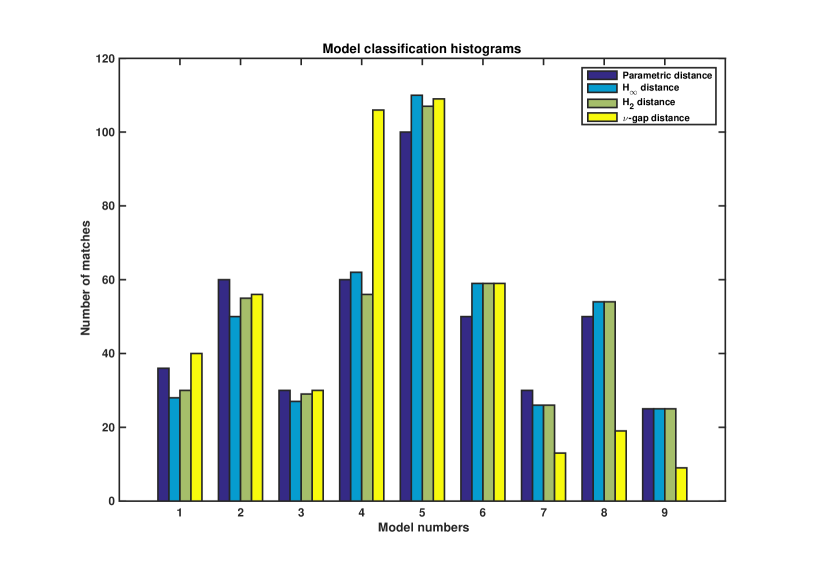
Figure 4: Classification of 441 models using different distances: parametric distance (dark blue), $\mathcal{H}_{\infty}$-norm (blue), $\mathcal{H}_{2}$-norm (green), $\nu$-gap distance (yellow)

The following MATLAB script produces the histogram in Fig. 4.

% Example - Comparison of estimations of minimum distances

% Define a lateral aircraft dynamics model with
% n  = 4 states, mu = 2 control inputs, p  = 4 measurable outputs
A = [-.4492 0.046 .0053 -.9926;
       0    0     1     0.0067;
   -50.8436 0   -5.2184  .722;
    16.4148 0     .0026 -.6627];
Bu = [0.0004 0.0011; 0 0; -1.4161 .2621; -0.0633 -0.1205];
C = eye(4); p = size(C,1); mu = size(Bu,2);

% define the loss of efficiency (LOE) faults as input scaling gains
% Gamma(i,:) = [ 1-rho1(i) 1-rho2(i) ]
Gamma = 1 - [ 0  0 0 .5 .5 .5 1  1 1;
              0 .5 1  0 .5  1 0 .5 1 ]’;
N = size(Gamma,1);  % number of LOE cases

% define a multiple physical fault model Gui = Gu*diag(Gamma(i,:))
sysu = ss(zeros(p,mu,N,1));
for i=1:N
    sysu(:,:,i,1) = ss(A,Bu*diag(Gamma(i,:)),C,0);
end
% setup the multiple model
sysu = mdmodset(sysu,struct(’controls’,1:mu));

% define fine grid and number of samples
rhogrid = 0:0.05:1; K = length(rhogrid)^2;
% perform least distance based model classification
ind = zeros(K,4);
i = 0;
for rho1 = rhogrid
    for rho2 = rhogrid
        i = i+1;
        % define actual model
        rho = [ rho1 rho2];
        sys = ss(A,Bu*diag(1-rho),C,0);
        set(sys,’InputGroup’,struct(’controls’,1:mu));
        temp = Gamma - repmat(1-rho,N,1);
        [~,ind(i,1)]   = min(sqrt(temp(:,1).^2+temp(:,2).^2));
        [~,~,ind(i,2)] = mddist2c(sysu,sys,struct(’distance’,’Inf’));
        [~,~,ind(i,3)] = mddist2c(sysu,sys,struct(’distance’,’2’));
        [~,~,ind(i,4)] = mddist2c(sysu,sys);
    end
end

% plot classification histograms
hist(ind,1:N)
title(’Model classification histograms’)
xlabel(’\bf Model numbers’)
ylabel(’\bf Number of matches’)
legend(’\bf Parametric distance’,’\bf H_\infty distance’,...
       ’\bf H_2 distance’,’\bf \nu-gap distance’)

4.6 Functions for Performance Evaluation of FDI Filters

These functions address the determination of the structure matrices defined in Section 2.5 and the computation of the performance criteria of FDI filters defined in Section 2.7. All functions are fully compatible with the results computed by the synthesis functions of FDI filters described in Section 4.8.

4.6.1 fditspec

Syntax

SMAT = fditspec(R)
SMAT = fditspec(R,TOL)
SMAT = fditspec(R,TOL,FDTOL)
SMAT = fditspec(R,TOL,FDTOL,FREQ)
SMAT = fditspec(R,TOL,FDTOL,[],BLKOPT)
SMAT = fditspec(R,TOL,FDTOL,FREQ,BLKOPT)

Description

fditspec determines the weak or strong structure matrix corresponding to the fault inputs of the internal form of a FDI filter or of a collection of internal forms of FDI filters.

Input data

R is a LTI system or a cell array of LTI systems.

If R is a LTI system representing the internal form of a FDI filter, then it is in a descriptor system state-space form

$$E_{R}\lambda x_{R}(t) =A_{R}x_{R}(t)+B_{R_{f}}f(t)+B_{R_{v}}v(t),$$ (91)

$$r(t) =C_{R}x_{R}(t)+D_{R_{f}}f(t)+D_{R_{v}}v(t),$$

where $r(t)\in\mathds{R}^{q}$ is the residual output, $f(t)\in\mathds{R}^{m_{f}}$ is the fault input and $v(t)$ contains all additional inputs. Any of the input components $f(t)$ and $v(t)$ can be void. For the fault input $f(t)$ the input group ’faults’ has to be defined. If there is no input group ’faults’ defined, then, by default, all system inputs are considered faults and the auxiliary input is assumed void. The input-output form of R corresponding to (91) is

$${\mathbf{r}}(\lambda)=R_{f}(\lambda){\mathbf{f}}(\lambda)+R_{v}(\lambda){\mathbf{v}}(\lambda),$$ (92)

where $R_{f}(\lambda)$ and $R_{v}(\lambda)$ are the transfer function matrices from the corresponding inputs, respectively. If R is specified in the input-output representation (92), then it is automatically converted to an equivalent minimal order state-space form as in (91).

If R is a $N\times 1$ cell array of LTI systems representing the internal forms of $N$ FDI filters, then the $i$-th component system R{$i$} is in the state-space form

$$E_{R}^{(i)}\lambda x_{R}^{(i)}(t) =A_{R}^{(i)}x_{R}^{(i)}(t)+B_{R_{f}}^{(i)}f(t)+B_{R_{v}}^{(i)}v(t),$$ (93)

$$r^{(i)}(t) =C_{R}^{(i)}x_{R}^{(i)}(t)+D_{R_{f}}^{(i)}f(t)+D_{R_{v}}^{(i)}v(t),$$

where $r^{(i)}(t)\in\mathds{R}^{q^{(i)}}$ is the $i$-th residual component, $f(t)\in\mathds{R}^{m_{f}}$ is the fault input and $v(t)$ contains the rest of inputs. Any of the input components $f(t)$ and $v(t)$ can be void. For the fault input $f(t)$ the input group ’faults’ has to be defined, while $v(t)$ includes any other (not relevant) system inputs. If there is no input group ’faults’ defined, then, by default, all system inputs are considered faults and the auxiliary input is assumed void. All component systems R{$i$}, $i=1,\ldots,N$, must have the same number of fault inputs and the same sampling time. The input-output form of R{$i$} corresponding to (93) is

$${\mathbf{r}}^{(i)}(\lambda)=R_{f}^{(i)}(\lambda){\mathbf{f}}(\lambda)+R_{v}^{(i)}(\lambda){\mathbf{v}}(\lambda),$$ (94)

where $R_{f}^{(i)}(\lambda)$ and $R_{v}^{(i)}(\lambda)$ are the transfer function matrices from the corresponding inputs, respectively. If R{$i$} is specified in the input-output representation (94), then it is automatically converted to an equivalent minimal order state-space form as in (93).

TOL is a relative tolerance used for controllability tests. A default value is internally computed if TOL $\leq 0$ or is not specified at input.

FDTOL is an absolute threshold for the magnitudes of the zero elements in the system matrices $B_{R_{f}}$, $C_{R}$ and $D_{R_{f}}$, in the case of model (91), or in the matrices $B_{R_{f}}^{(i)}$, $C_{R}^{(i)}$ and $D_{R_{f}}^{(i)}$, in the case of models of the form (93). Any element of these matrices whose magnitude does not exceed FDTOL is considered zero. Additionally, if FREQ is nonempty, FDTOL is also used for the singular-value-based rank tests performed on the system matrix $\Big{[}\begin{smallmatrix}A_{R}-\lambda E_{R}&B_{R_{f}}\\ C_{R}&D_{R_{f}}\end{smallmatrix}\Big{]}$, in the case of model (91), or on the system matrices $\bigg{[}\begin{smallmatrix}A_{R}^{(i)}-\lambda E_{R}^{(i)}&B_{R_{f}}^{(i)}\\ C_{R}^{(i)}&D_{R_{f}}^{(i)}\end{smallmatrix}\bigg{]}$ for $i=1,\ldots,N$, in the case of models of the form (93). If FDTOL $\leq 0$ or not specified at input, the default value FDTOL = $10^{-4}\max\big{(}1,\big{\|}B_{R_{f}}\big{\|}_{1},\big{\|}C_{R}\big{\|}_{\infty},\big{\|}D_{R_{f}}\big{\|}_{1}\big{)}$ is used in the case of model (91). In the case of models of the form (93), the default value FDTOL = $10^{-4}\max\big{(}1,\big{\|}B_{R_{f}}^{(i)}\big{\|}_{1},\big{\|}C_{R}^{(i)}\big{\|}_{\infty},\big{\|}D_{R_{f}}^{(i)}\big{\|}_{1}\big{)}$ is used for handling the $i$-th model (93). If FDTOL $\leq 0$ and if FREQ is nonempty, the default value FDTOL = $10^{-4}\max\Big{(}1,\Big{\|}\left[\begin{smallmatrix}A_{R}&B_{R_{f}}\\ C_{R}&D_{R_{f}}\end{smallmatrix}\right]\Big{\|}_{1},\big{\|}E_{R}\big{\|}_{1}\Big{)}$ is used for the rank tests on the system matrix in the case of model (91). In the case of models of the form (93), the default value FDTOL = $10^{-4}\max\Big{(}1,\Bigg{\|}\left[\begin{smallmatrix}A_{R}^{(i)}&B_{R_{f}}^{(i)}\\ C_{R}^{(i)}&D_{R_{f}}^{(i)}\end{smallmatrix}\right]\Bigg{\|}_{1},\big{\|}E_{R}^{(i)}\big{\|}_{1}\Big{)}$ is used for handling the system matrix of the $i$-th model (93).

FREQ is a real vector, which contains the frequency values $\omega_{k}$, $k=1,\ldots,n_{f}$, to be used to check for zeros of the individual (rational) elements or individual columns of the transfer function matrix $R_{f}(\lambda)$ in the case of model (91), or of the transfer function matrices $R_{f}^{(i)}(\lambda)$ in the case of models (93). By default, FREQ is empty if it is not specified. For each real frequency $\omega_{k}$ contained in FREQ, there corresponds a complex frequency $\lambda_{k}$, which is used to check the elements or columns of the respective transfer function matrices to have $\lambda_{k}$ as zero. Depending on the system type, $\lambda_{k}=\mathrm{i}\omega_{k}$, in the continuous-time case, and $\lambda_{k}=\exp(\mathrm{i}\omega_{k}T)$, in the discrete-time case, where $T$ is the sampling time of the system.

BLKOPT is a character variable to be set to ’block’ to specify the block-structure based evaluation option of the structure matrix.

Output data

SMAT is a logical array which contains the resulting structure matrix.

In the case of a LTI system R, SMAT is determined depending on the selected option BLKOPT and the frequency values specified in FREQ, as follows:

• If BLKOPT is not specified (or empty), then SMAT is the structure matrix corresponding to the zero and nonzero elements of the transfer function matrix $R_{f}(\lambda)$:

  • If FREQ is empty or not specified at input, then SMAT is a $q\times m_{f}$ logical array, which contains the weak structure matrix corresponding to the zero and nonzero elements of $R_{f}(\lambda)$ (see (14) for the definition of the weak structure matrix). Accordingly, SMAT$(i,j)$ = true, if the $(i,j)$-th element of $R_{f}(\lambda)$ is nonzero. Otherwise, SMAT$(i,j)$ = false.

  • If FREQ is nonempty, then SMAT is a $q\times m_{f}\times n_{f}$ logical array which contains in the $k$-th page $\texttt{SMAT}(:,:,k)$, the strong structure matrix corresponding to the presence or absence of zeros of the elements of $R_{f}(\lambda)$ in the complex frequency $\lambda_{k}$ corresponding to the $k$-th real frequency $\omega_{k}$ contained in FREQ (see description of FREQ) (see also (18) for the definition of the strong structure matrix at a complex frequency $\lambda_{k}$). Accordingly, $\texttt{SMAT}(i,j,k)$ = true, if the $(i,j)$-th element of $R_{f}(\lambda)$ has no zero in $\lambda_{k}$. Otherwise, $\texttt{SMAT}(i,j,k)$ = false.

• If BLKOPT = ’block’ is specified, then SMAT is the structure (row) vector corresponding to the zero and nonzero columns of the transfer function matrix $R_{f}(\lambda)$:

  • If FREQ is empty or not specified at input, then SMAT is a $1\times m_{f}$ logical (row) vector, which contains the weak structure matrix corresponding to the zero and nonzero columns of $R_{f}(\lambda)$ (see (14) for the block-structured definition of the weak structure matrix). Accordingly, SMAT$(1,j)$ = true, if the $j$-th column of $R_{f}(\lambda)$ is nonzero. Otherwise, SMAT$(1,j)$ = false.

  • If FREQ is nonempty, then SMAT is a $1\times m_{f}\times n_{f}$ logical array which contains in the $k$-th page $\texttt{SMAT}(:,:,k)$, the strong structure vector corresponding to the presence or absence of a zero in the columns of $R_{f}(\lambda)$ in the complex frequency $\lambda_{k}$ corresponding to the $k$-th real frequency $\omega_{k}$ contained in FREQ (see description of FREQ). Accordingly, $\texttt{SMAT}(1,j,k)$ = true, if the $j$-th column of $R_{f}(\lambda)$ has no zero in the complex frequency $\lambda_{k}$. Otherwise, $\texttt{SMAT}(1,j,k)$ = false.

In the case of a cell array of LTI systems R{$i$}, $i=1,\ldots,N$, SMAT is determined depending on the frequency values specified in FREQ, as follows:

• If FREQ is empty or not specified at input, then SMAT is an $N\times m_{f}$ logical matrix, whose $i$-th row contains the weak structure vector corresponding to the zero and nonzero columns of the transfer function matrix $R_{f}^{(i)}(\lambda)$ (see (14) for the block-structured definition of the weak structure matrix). Accordingly, SMAT$(i,j)$ = true, if the $j$-th column of $R_{f}^{(i)}(\lambda)$ is nonzero. Otherwise, SMAT$(i,j)$ = false. All entries of the $i$-th row of SMAT are set to false if R{$i$} is empty.

• If FREQ is nonempty, then SMAT is a $N\times m_{f}\times n_{f}$ logical array which contains in the $i$-th row of the $k$-th page $\texttt{SMAT}(:,:,k)$, the strong structure (row) vector corresponding to the presence or absence of a zero in the columns of $R_{f}^{(i)}(\lambda)$ in the complex frequency $\lambda_{k}$ corresponding to the $k$-th real frequency $\omega_{k}$ contained in FREQ (see description of FREQ) (see also (18) for the definition of the strong structure matrix at a complex frequency $\lambda_{k}$). Accordingly, $\texttt{SMAT}(i,j,k)$ = true, if the $j$-th column of $R_{f}^{(i)}(\lambda)$ has no zero in $\lambda_{k}$. Otherwise, $\texttt{SMAT}(i,j,k)$ = false. All entries of the $i$-th row of SMAT are set to false if R{$i$} is empty.

Method

We first describe the implemented analysis method for the case when R is a LTI system in a state-space form as in (91) and $R_{f}(\lambda)$ is the transfer function matrix from the fault inputs to the residual output as in the input-output model (92). For the definition of the weak and strong structure matrices, see Section 2.5. For the determination of the weak structure matrix, controllable realizations are determined for each column of $R_{f}(\lambda)$ and tests are performed to identify the nonzero elements in the respective column of $R_{f}(\lambda)$ by using [16, Corollary 7.1] in a controllability related dual formulation. The block-structure based evaluation is based on the input observability tests of [16, Corollary 7.1], performed for the controllable realizations of each column of $R_{f}(\lambda)$.

For the determination of the strong structure matrix, minimal realizations are determined for each element of $R_{f}(\lambda)$ and the absence of zeros is assessed by checking the full rank of the corresponding system matrix for all complex frequencies corresponding to the real frequencies specified in FREQ (see [16, Corollary 7.2]). For the block-structure based evaluation, controllable realizations are determined for each column of $R_{f}(\lambda)$ and the test used in [16, Corollary 7.2] is employed.

For the case when R is a cell array containing $N$ LTI systems in state-space forms as in (93) and $R_{f}^{(i)}(\lambda)$ is the transfer function matrix of $i$-th LTI system R{$i$} from the fault inputs to the $i$-th residual component as in the input-output models (94), the block-structure based evaluations, described above, are employed for each $R_{f}^{(i)}(\lambda)$ to determine the corresponding $i$-th row of the structure matrix SMAT.

4.6.2 fdisspec

Syntax

[SMAT,GAINS] = fdisspec(R)
[SMAT,GAINS] = fdisspec(R,FDGAINTOL)
[SMAT,GAINS] = fdisspec(R,FDGAINTOL,FREQ)
[SMAT,GAINS] = fdisspec(R,FDGAINTOL,FREQ,BLKOPT)

Description

fdisspec determines the strong structure matrix corresponding to the fault inputs of the internal form of a FDI filter or of a collection of internal forms of FDI filters.

Input data

R is a LTI system or a cell array of LTI systems.

If R is a LTI system representing the internal form of a FDI filter, then it is in a descriptor system state-space form

$$E_{R}\lambda x_{R}(t) =A_{R}x_{R}(t)+B_{R_{f}}f(t)+B_{R_{v}}v(t),$$ (95)

$$r(t) =C_{R}x_{R}(t)+D_{R_{f}}f(t)+D_{R_{v}}v(t),$$

where $r(t)\in\mathds{R}^{q}$ is the residual output, $f(t)\in\mathds{R}^{m_{f}}$ is the fault input and $v(t)$ contains all additional inputs. Any of the input components $f(t)$ and $v(t)$ can be void. For the fault input $f(t)$ the input group ’faults’ has to be defined. If there is no input group ’faults’ defined, then, by default, all system inputs are considered faults and the auxiliary input is assumed void. The input-output form of R corresponding to (95) is

$${\mathbf{r}}(\lambda)=R_{f}(\lambda){\mathbf{f}}(\lambda)+R_{v}(\lambda){\mathbf{v}}(\lambda),$$ (96)

where $R_{f}(\lambda)$ and $R_{v}(\lambda)$ are the transfer function matrices from the corresponding inputs. If R is specified in the input-output representation (96), then it is automatically converted to an equivalent minimal order state-space form as in (95).

If R is an $N\times 1$ cell array of LTI systems representing the internal forms of $N$ FDI filters, then the $i$-th component system R{$i$} is in the state-space form

$$E_{R}^{(i)}\lambda x_{R}^{(i)}(t) =A_{R}^{(i)}x_{R}^{(i)}(t)+B_{R_{f}}^{(i)}f(t)+B_{R_{v}}^{(i)}v(t),$$ (97)

$$r^{(i)}(t) =C_{R}^{(i)}x_{R}^{(i)}(t)+D_{R_{f}}^{(i)}f(t)+D_{R_{v}}^{(i)}v(t),$$

where $r^{(i)}(t)\in\mathds{R}^{q^{(i)}}$ is the $i$-th residual component, $f(t)\in\mathds{R}^{m_{f}}$ is the fault input and $v(t)$ contains the rest of inputs. Any of the input components $f(t)$ and $v(t)$ can be void. For the fault input $f(t)$ the input group ’faults’ has to be defined, while $v(t)$ includes any other (not-relevant) system inputs. If there is no input group ’faults’ defined, then, by default, all system inputs are considered faults and the auxiliary input is assumed void. All component systems R{$i$}, $i=1,\ldots,N$, must have the same number of fault inputs and the same sampling time. The input-output form of R{$i$} corresponding to (97) is

$${\mathbf{r}}^{(i)}(\lambda)=R_{f}^{(i)}(\lambda){\mathbf{f}}(\lambda)+R_{v}^{(i)}(\lambda){\mathbf{v}}(\lambda),$$ (98)

where $R_{f}^{(i)}(\lambda)$ and $R_{v}^{(i)}(\lambda)$ are the transfer function matrices from the corresponding inputs. If R{$i$} is specified in the input-output representation (98), then it is automatically converted to an equivalent minimal order state-space form as in (97).

FDGAINTOL is a threshold for the magnitudes of the frequency-response gains of the transfer function matrix $R_{f}(\lambda)$ in the case of model (95), or of the transfer function matrices $R_{f}^{(i)}(\lambda)$ in the case of models (97). If FDGAINTOL = 0 or not specified at input, the default value FDGAINTOL = 0.01 is used.

FREQ is a real vector, which contains the real frequency values $\omega_{k}$, $k=1,\ldots,n_{f}$, to be used to check for the existence of zeros of the (rational) elements or columns of the transfer function matrix $R_{f}(\lambda)$ in the case of model (91), or of the transfer function matrices $R_{f}^{(i)}(\lambda)$ in the case of models (93). By default, FREQ = 0, if it is empty or not specified. For each real frequency $\omega_{k}$ contained in FREQ, there corresponds a complex frequency $\lambda_{k}$ which is used to evaluate $R_{f}(\lambda_{k})$, to check that the elements or columns of the respective transfer function matrices have $\lambda_{k}$ as a zero. Depending on the system type, $\lambda_{k}=\mathrm{i}\omega_{k}$, in the continuous-time case, and $\lambda_{k}=\exp(\mathrm{i}\omega_{k}T)$, in the discrete-time case, where $T$ is the sampling time of the system. The complex frequencies corresponding to the real frequencies specified in FREQ must be disjoint from the set of poles of $R_{f}(\lambda)$.

BLKOPT is a character variable to be set to ’block’ to specify the block-structure based evaluation option of the structure matrix.

Output data

SMAT is a logical array which contains the resulting structure matrix.

In the case R is a LTI system, SMAT is determined depending on the selected option BLKOPT, as follows:

• If BLKOPT is not specified (or empty), then SMAT is a $q\times m_{f}\times n_{f}$ logical array which contains in the $k$-th page $\texttt{SMAT}(:,:,k)$, the strong structure matrix corresponding to the presence or absence of zeros of the elements of $R_{f}(\lambda)$ in the complex frequency $\lambda_{k}$ corresponding to the $k$-th real frequency $\omega_{k}$ contained in FREQ (see description of FREQ) (see also (18) for the definition of the strong structure matrix at a complex frequency $\lambda_{k}$). Accordingly, $\texttt{SMAT}(i,j,k)$ = true, if the magnitude of the $(i,j)$-th element of $R_{f}(\lambda_{k})$ is greater than or equal to FDGAINTOL. Otherwise, $\texttt{SMAT}(i,j,k)$ = false.

• If BLKOPT = ’block’ is specified, then SMAT is a $1\times m_{f}\times n_{f}$ logical array which contains in the $k$-th page $\texttt{SMAT}(:,:,k)$, the strong structure (row) vector corresponding to the presence or absence of a zero in the columns of $R_{f}(\lambda)$ in the complex frequency $\lambda_{k}$ corresponding to the $k$-th real frequency $\omega_{k}$ contained in FREQ (see description of FREQ). Accordingly, $\texttt{SMAT}(1,j,k)$ = true, if the norm of the $j$-th column of $R_{f}(\lambda_{k})$ is greater than or equal to FDGAINTOL (i.e., $\big{\|}R_{f_{j}}(\lambda_{k})\big{\|}_{2}\geq$ FDGAINTOL). Otherwise, $\texttt{SMAT}(1,j,k)$ = false.

In the case R is an $N\times 1$ cell array of LTI systems, SMAT is an $N\times m_{f}\times n_{f}$ logical array which contains in the $i$-th row of the $k$-th page $\texttt{SMAT}(:,:,k)$, the strong structure (row) vector corresponding to the presence or absence of a zero in the columns of $R_{f}^{(i)}(\lambda)$ in the complex frequency $\lambda_{k}$ corresponding to the $k$-th real frequency $\omega_{k}$ contained in FREQ (see description of FREQ) (see also (18) for the definition of the strong structure matrix at a complex frequency $\lambda_{k}$). Accordingly, $\texttt{SMAT}(i,j,k)$ = true, if the norm of the $j$-th column of $R_{f}^{(i)}(\lambda_{k})$ is greater than or equal to FDGAINTOL (i.e., $\big{\|}R_{f_{j}}^{(i)}(\lambda_{k})\big{\|}_{2}\geq$ FDGAINTOL). Otherwise, $\texttt{SMAT}(i,j,k)$ = false. If R{$i$} is empty, then all entries of the $i$-th row of SMAT are set to false.

GAINS is a real nonnegative array.

In the case R is a LTI system, GAINS is determined depending on the selected option BLKOPT, as follows:

• If BLKOPT is not specified (or empty), then GAINS is $q\times m_{f}$ matrix, whose $(i,j)$-th element contains the minimum value of the frequency-response gains of the $(i,j)$-th element of $R_{f}(\lambda)$ evaluated over all complex frequencies corresponding to FREQ (see description of FREQ). This value is a particular instance of the $\mathcal{H}_{-}$-index of the $(i,j)$-th element of $R_{f}(\lambda)$.

• If BLKOPT = ’block’ is specified, then GAINS is a $m_{f}$-dimensional row vector, whose $j$-th element contains the minimum of the norms of the frequency responses of the $j$-th column of $R_{f}(\lambda)$ evaluated over all complex frequencies corresponding to FREQ (see description of FREQ). This value is a particular instance of the $\mathcal{H}_{-}$-index of the $j$-th column of $R_{f}(\lambda)$.

In the case R is an $N\times 1$ cell array of LTI systems, GAINS is an $N\times m_{f}$ matrix, whose $(i,j)$-th element contains the minimum of the norms of the frequency responses of the $j$-th column of $R_{f}^{(i)}(\lambda)$ evaluated over all complex frequencies corresponding to FREQ (see description of FREQ). If R{$i$} is empty, then all entries of the $i$-th row of GAINS are set to zero.

Method

For the definition of the strong structure matrix at a given frequency, see Remark 3 of Section 2.5. For the case when R is a LTI system in a state-space form as in (95) and $R_{f}(\lambda)$ is the transfer function matrix from the fault inputs to the residual output as in the input-output model (96), the element-wise or column-wise (if BLKOPT = ’block’) evaluations of the $\mathcal{H}_{-}$-index on a discrete set of frequency values (see [16, Section 5.3]) are employed for each element or, respectively, each column of $R_{f}(\lambda)$, to determine the corresponding element of the structure matrix SMAT and associated GAINS. The resulting entries of GAINS correspond to an element-wise or column-wise evaluation of the $\mathcal{H}_{-}$-index on a discrete set of frequency values (see [16, Section 5.3]).

For the case when R is a cell array containing $N$ LTI systems in state-space forms as in (97) and $R_{f}^{(i)}(\lambda)$ is the transfer function matrix of $i$-th LTI system R{$i$} from the fault inputs to the $i$-th residual component as in the input-output models (98), the column-wise evaluations of the $\mathcal{H}_{-}$-index on a discrete set of frequency values (see [16, Section 5.3]) are employed for each $R_{f}^{(i)}(\lambda)$ to determine the corresponding $i$-row of the structure matrix SMAT and the associated $i$-th row of GAINS.

4.6.3 fdifscond

Syntax

FSCOND = fdifscond(R)
FSCOND = fdifscond(R,FREQ)
FSCOND = fdifscond(R,[],S)
FSCOND = fdifscond(R,FREQ,S)
[BETA,GAMMA] = fdifscond(...)

Description

fdifscond evaluates the fault sensitivity condition of the internal form of a FDI filter or the fault sensitivity conditions of the internal forms of a collection of FDI filters.

Input data

R is a LTI system or a cell array of LTI systems.

If R is a LTI system representing the internal form of a FDI filter, then it is in a descriptor system state-space form

$$E_{R}\lambda x_{R}(t) =A_{R}x_{R}(t)+B_{R_{f}}f(t)+B_{R_{v}}v(t),$$ (99)

$$r(t) =C_{R}x_{R}(t)+D_{R_{f}}f(t)+D_{R_{v}}v(t),$$

where $r(t)\in\mathds{R}^{q}$ is the residual output, $f(t)\in\mathds{R}^{m_{f}}$ is the fault input, and $v(t)$ contains all additional inputs. For the fault input $f(t)$ the input group ’faults’ has to be defined. The input-output form of R corresponding to (99) is

$${\mathbf{r}}(\lambda)=R_{f}(\lambda){\mathbf{f}}(\lambda)+R_{v}(\lambda){\mathbf{v}}(\lambda),$$ (100)

where $R_{f}(\lambda)$ and $R_{v}(\lambda)$ are the transfer function matrices from the corresponding inputs.

If R is an $N\times 1$ cell array of LTI systems representing the internal forms of $N$ FDI filters, then the $i$-th component system R{$i$} is in the state-space form

$$E_{R}^{(i)}\lambda x_{R}^{(i)}(t) =A_{R}^{(i)}x_{R}^{(i)}(t)+B_{R_{f}}^{(i)}f(t)+B_{R_{v}}^{(i)}v(t),$$ (101)

$$r^{(i)}(t) =C_{R}^{(i)}x_{R}^{(i)}(t)+D_{R_{f}}^{(i)}f(t)+D_{R_{v}}^{(i)}v(t),$$

where $r^{(i)}(t)\in\mathds{R}^{q^{(i)}}$ is the $i$-th residual component, $f(t)\in\mathds{R}^{m_{f}}$ is the fault input and $v(t)$ contains the rest of inputs. For the fault input $f(t)$ the input group ’faults’ has to be defined. The input-output form of R{$i$} corresponding to (101) is

$${\mathbf{r}}^{(i)}(\lambda)=R_{f}^{(i)}(\lambda){\mathbf{f}}(\lambda)+R_{v}^{(i)}(\lambda){\mathbf{v}}(\lambda),$$ (102)

where $R_{f}^{(i)}(\lambda)$ and $R_{v}^{(i)}(\lambda)$ are the transfer function matrices from the corresponding inputs.

FREQ is a real vector, which contains the frequency values $\omega_{k}$, $k=1,\ldots,n_{f}$, to be used to evaluate the fault condition number of the transfer function matrix $R_{f}(\lambda)$ in (100), or of the transfer function matrices $R_{f}^{(i)}(\lambda)$ in (102). By default, FREQ is empty if it is not specified. For each real frequency $\omega_{k}$ contained in FREQ, there corresponds a complex frequency $\lambda_{k}$, which is used to define the complex set $\Omega=\{\lambda_{1},\ldots,\lambda_{n_{f}}\}$. Depending on the system type, $\lambda_{k}=\mathrm{i}\omega_{k}$, in the continuous-time case, and $\lambda_{k}=\exp(\mathrm{i}\omega_{k}T)$, in the discrete-time case, where $T$ is the sampling time of the system.

S is a $q\times m_{f}$ logical structure matrix if R is the internal form of a FDI filter with $q$ residual outputs or is an $N\times m_{f}$ logical structure matrix if R is a collection of $N$ internal forms of fault detection and isolation filters, where R$\{i\}$ is the internal form of the $i$-th filter.

Output data

FSCOND is the computed fault sensitivity condition, which is either a scalar or a vector, depending on the input variables.

In the case of calling fdifscond as

   FSCOND = fdifscond(R)

then:

• If R is a LTI system, then FSCOND is the fault sensitivity condition computed as $\beta/\gamma$, where $\beta=\|R_{\!f}(\lambda)\|_{\infty-}$ and $\gamma=\displaystyle\max_{j}\|R_{\!f_{j}}(\lambda)\|_{\infty}$ ;

• If R is a collection of $N$ LTI systems, then FSCOND is an $N$-dimensional vector of fault sensitivity conditions, with FSCOND{$i$}, the $i$-th fault sensitivity condition, computed as $\beta_{i}/\gamma_{i}$, where $\beta_{i}=\|R_{\!f}^{(i)}(\lambda)\|_{\infty-}$ and $\gamma_{i}=\displaystyle\max_{j}\|R_{\!f_{j}}^{(i)}(\lambda)\|_{\infty}$. If R{$i$} is empty, then FSCOND{$i$} is set to NaN.

In the case of calling fdifscond as

   FSCOND = fdifscond(R,FREQ)

where FREQ is a nonempty vector of real frequencies, which define the set of complex frequencies $\Omega$ (see description of FREQ), then:

• If R is a LTI system, then FSCOND is the fault sensitivity condition computed as $\beta/\gamma$, where $\beta=\big{\|}R_{\!f}(\lambda)\big{\|}_{\Omega-}$ and $\gamma=\displaystyle\max_{j}\big{\{}\sup_{\lambda_{s}\in\Omega}\big{\|}R_{\!f_{j}}(\lambda_{s})\big{\|}_{2}\big{\}}$ ;

• If R is a collection of $N$ LTI systems, then FSCOND is an $N$-dimensional vector of fault sensitivity conditions, with FSCOND{$i$}, the $i$-th fault sensitivity condition, computed as $\beta_{i}/\gamma_{i}$, where $\beta_{i}=\big{\|}R_{\!f}^{(i)}(\lambda)\big{\|}_{\Omega-}$ and $\gamma_{i}=\displaystyle\max_{j}\big{\{}\sup_{\lambda_{s}\in\Omega}\big{\|}R_{\!f_{j}}^{(i)}(\lambda_{s})\big{\|}_{2}\big{\}}$. If R{$i$} is empty, then FSCOND{$i$} is set to NaN.

In the case of calling fdifscond as

   FSCOND = fdifscond(R,[],S)

then:

• If R is a LTI system with $q$ residual outputs and S is a $q\times m_{f}$ structure matrix, then FSCOND is a $q$-dimensional vector of fault sensitivity conditions. FSCOND{$i$} is the fault sensitivity condition of the $i$-th row $R_{\!f}^{(i)}(\lambda)$ of $R_{\!f}(\lambda)$, computed as $\beta_{i}/\gamma_{i}$, with $\beta_{i}=\big{\|}R_{\!f^{(i)}}^{(i)}(\lambda)\big{\|}_{\infty-}$ and $\gamma_{i}=\displaystyle\max_{j}\big{\|}R_{\!f_{j}}^{(i)}(\lambda)\big{\|}_{\infty}$, where $R_{\!f^{(i)}}^{(i)}(\lambda)$ is formed from the elements of $R_{\!f}^{(i)}(\lambda)$ which correspond to true values in the $i$-th row of S and $R_{\!f_{j}}^{(i)}(\lambda)$ is the $(i,j)$-th element of $R_{\!f}(\lambda)$;

• If R is a collection of $N$ LTI systems and S is an $N\times m_{f}$ structure matrix, then FSCOND is an $N$-dimensional vector of fault sensitivity conditions, with FSCOND{$i$}, the $i$-th fault sensitivity condition, computed as $\beta_{i}/\gamma_{i}$, with $\beta_{i}=\big{\|}R_{\!f^{(i)}}^{(i)}(\lambda)\big{\|}_{\infty-}$ and $\gamma_{i}=\displaystyle\max_{j}\big{\|}R_{\!f_{j}}^{(i)}(\lambda)\big{\|}_{\infty}$, where $R_{\!f^{(i)}}^{(i)}(\lambda)$ is formed from the columns of $R_{\!f}^{(i)}(\lambda)$ which correspond to true values in the $i$-th row of S and $R_{\!f_{j}}^{(i)}(\lambda)$ is the $j$-th column of $R_{\!f}^{(i)}(\lambda)$. If R{$i$} is empty, then FSCOND{$i$} is set to NaN.

In the case of calling fdifscond as

   FSCOND = fdifscond(R,FREQ,S)

where both FREQ and S are nonempty then:

• If R is a LTI system with $q$ residual outputs and S is a $q\times m_{f}$ structure matrix, then FSCOND is a $q$-dimensional vector of fault sensitivity conditions. FSCOND{$i$} is the fault sensitivity condition of the $i$-th row $R_{\!f}^{(i)}(\lambda)$ of $R_{\!f}(\lambda)$, computed as $\beta_{i}/\gamma_{i}$, with $\beta_{i}=\big{\|}R_{\!f^{(i)}}^{(i)}(\lambda)\big{\|}_{\Omega-}$ and $\gamma_{i}=\displaystyle\max_{j}\big{\{}\sup_{\lambda_{s}\in\Omega}\big{\|}R_{\!f_{j}}^{(i)}(\lambda_{s})\big{\|}_{2}\big{\}}$, where $R_{\!f^{(i)}}^{(i)}(\lambda)$ is formed from the elements of $R_{\!f}^{(i)}(\lambda)$ which correspond to true values in the $i$-th row of S and $R_{\!f_{j}}^{(i)}(\lambda)$ is the $(i,j)$-th element of $R_{\!f}(\lambda)$;

• If R is a collection of $N$ LTI systems and S is an $N\times m_{f}$ structure matrix, then FSCOND is an $N$-dimensional vector of fault sensitivity conditions. FSCOND{$i$} is the fault sensitivity condition of the $i$-th system R{$i$}, computed as $\beta_{i}/\gamma_{i}$, with $\beta_{i}=\big{\|}R_{\!f^{(i)}}^{(i)}(\lambda)\big{\|}_{\Omega-}$ and $\gamma_{i}=\displaystyle\max_{j}\big{\{}\sup_{\lambda_{s}\in\Omega}\big{\|}R_{\!f_{j}}^{(i)}(\lambda_{s})\big{\|}_{2}\big{\}}$, where $R_{\!f^{(i)}}^{(i)}(\lambda)$ is formed from the columns of $R_{\!f}^{(i)}(\lambda)$ which correspond to true values in the $i$-th row of S and $R_{\!f_{j}}^{(i)}(\lambda)$ is the $j$-th column of $R_{\!f}^{(i)}(\lambda)$. If R{$i$} is empty, then FSCOND{$i$} is set to NaN.

In the case of calling fdifscond as

   [BETA,GAMMA] = fdifscond(...)

then:

If BETA and GAMMA are scalar values, then they contain the values of $\beta$ and $\gamma$, respectively, whose ratio represents the fault sensitivity condition. If BETA and GAMMA are vectors, then BETA{$i$} and GAMMA{$i$} contain the values of $\beta_{i}$ and $\gamma_{i}$, respectively, whose ratio represents the $i$-th fault sensitivity condition. If R{$i$} is empty, then BETA{$i$} and GAMMA{$i$} are set to zero.

Method

The definitions of the fault sensitivity condition in terms of the $\mathcal{H}_{\infty-}$-index and its finite frequency counterpart, the $\mathcal{H}_{\Omega-}$-index, are given in Section 2.7.1.

4.6.4 fdif2ngap

Syntax

GAP = fdif2ngap(R)
GAP = fdif2ngap(R,FREQ)
GAP = fdif2ngap(R,[],S)
GAP = fdif2ngap(R,FREQ,S)
[BETA,GAMMA] = fdif2ngap(...)

Description

fdif2ngap evaluates the fault-to-noise gap of the internal form of a FDI filter or the fault-to-noise gaps of the internal forms of a collection of FDI filters.

Input data

R is a LTI system or a cell array of LTI systems.

If R is a LTI system representing the internal form of a FDI filter, then it is in a descriptor system state-space form

$$E_{R}\lambda x_{R}(t) =A_{R}x_{R}(t)+B_{R_{f}}f(t)+B_{R_{w}}w(t)+B_{R_{v}}v(t),$$ (103)

$$r(t) =C_{R}x_{R}(t)+D_{R_{f}}f(t)+D_{R_{w}}w(t)+D_{R_{v}}v(t),$$

where $r(t)\in\mathds{R}^{q}$ is the residual output, $f(t)\in\mathds{R}^{m_{f}}$ is the fault input, $w(t)\in\mathds{R}^{m_{w}}$ is the noise input and $v(t)$ is the auxiliary input. For the fault input $f(t)$ and noise input $w(t)$ the input groups ’faults’ and ’noise’, respectively, have to be defined. The input-output form of R corresponding to (103) is

$${\mathbf{y}}(\lambda)=G_{f}(\lambda){\mathbf{f}}(\lambda)+G_{w}(\lambda){\mathbf{w}}(\lambda)+G_{v}(\lambda){\mathbf{v}}(\lambda),$$ (104)

where $R_{f}(\lambda)$, $R_{w}(\lambda)$ and $R_{v}(\lambda)$ are the transfer function matrices from the corresponding inputs.

If R is an $N\times 1$ cell array of LTI systems representing the internal forms of $N$ FDI filters, then the $i$-th component system R{$i$} is in the state-space form

$$E_{R}^{(i)}\lambda x_{R}^{(i)}(t) =A_{R}^{(i)}x_{R}^{(i)}(t)+B_{R_{f}}^{(i)}f(t)+B_{R_{w}}^{(i)}w(t),$$ (105)

$$r^{(i)}(t) =C_{R}^{(i)}x_{R}^{(i)}(t)+D_{R_{f}}^{(i)}f(t)+D_{R_{w}}^{(i)}w(t),$$

where $r^{(i)}(t)\in\mathds{R}^{q^{(i)}}$ is the $i$-th residual component, $f(t)\in\mathds{R}^{m_{f}}$ is the fault input and $w(t)$ is the noise input. For the fault input $f(t)$ and noise input $w(t)$ the input groups ’faults’ and ’noise’, respectively, have to be defined. The input-output form of R{$i$} corresponding to (105) is

$${\mathbf{r}}^{(i)}(\lambda)=R_{f}^{(i)}(\lambda){\mathbf{f}}(\lambda)+R_{w}^{(i)}(\lambda){\mathbf{w}}(\lambda),$$ (106)

where $R_{f}^{(i)}(\lambda)$ and $R_{w}^{(i)}(\lambda)$ are the transfer function matrices from the corresponding inputs.

FREQ is a real vector, which contains the frequency values $\omega_{k}$, $k=1,\ldots,n_{f}$, to be used to evaluate the gap between the transfer function matrices $R_{f}(\lambda)$ and $R_{w}(\lambda)$ in (104), or between the transfer function matrices $R_{f}^{(i)}(\lambda)$ and $R_{w}^{(i)}(\lambda)$ in (106). By default, FREQ is empty if it is not specified. For each real frequency $\omega_{k}$ contained in FREQ, there corresponds a complex frequency $\lambda_{k}$, which is used to define the complex set $\Omega=\{\lambda_{1},\ldots,\lambda_{n_{f}}\}$. Depending on the system type, $\lambda_{k}=\mathrm{i}\omega_{k}$, in the continuous-time case, and $\lambda_{k}=\exp(\mathrm{i}\omega_{k}T)$, in the discrete-time case, where $T$ is the sampling time of the system.

S is a $q\times m_{f}$ logical structure matrix if R is the internal form of fault detection filter with $q$ residual outputs or is an $N\times m_{f}$ logical structure matrix if R is a collection of $N$ internal forms of fault detection and isolation filters, where R$\{i\}$ is the internal form of the $i$-th filter.

Output data

GAP is the computed fault-to-noise gap, which is either a scalar or a vector, depending on the input variables.

In the case of calling fdif2ngap as

   GAP = fdif2ngap(R)

then:

• If R is a LTI system, then GAP is the fault-to-noise gap computed as $\beta/\gamma$, where $\beta=\big{\|}R_{\!f}(\lambda)\big{\|}_{\infty-}$ and $\gamma=\big{\|}R_{w}(\lambda)\big{\|}_{\infty}$ ;

• If R is a collection of $N$ LTI systems, then GAP is an $N$-dimensional vector, with GAP{$i$}, the $i$-th fault-to-noise gap, computed as $\beta_{i}/\gamma_{i}$, where $\beta_{i}=\big{\|}R_{\!f}^{(i)}(\lambda)\big{\|}_{\infty-}$ and $\gamma_{i}=\big{\|}R_{w}^{(i)}(\lambda)\big{\|}_{\infty}$. If R{$i$} is empty, then GAP{$i$} is set to NaN.

In the case of calling fdif2ngap as

   GAP = fdif2ngap(R,FREQ)

where FREQ is a nonempty vector of real frequencies, which defines the set of complex frequencies $\Omega$ (see description of FREQ), then:

• If R is a LTI system, then GAP is the fault-to-noise gap computed as $\beta/\gamma$, where $\beta=\big{\|}R_{\!f}(\lambda)\big{\|}_{\Omega-}$ and $\gamma=\big{\|}R_{w}(\lambda)\big{\|}_{\infty}$ ;

• If R is a collection of $N$ LTI systems, then GAP is an $N$-dimensional vector, with GAP{$i$}, the $i$-th fault-to-noise gap, computed as $\beta_{i}/\gamma_{i}$, where $\beta_{i}=\big{\|}R_{\!f}^{(i)}(\lambda)\big{\|}_{\Omega-}$ and $\gamma_{i}=\big{\|}R_{w}^{(i)}(\lambda)\big{\|}_{\infty}$. If R{$i$} is empty, then GAP{$i$} is set to NaN.

In the case of calling fdif2ngap as

   GAP = fdif2ngap(R,[],S)

then:

• If R is a LTI system with $q$ residual outputs and S is a $q\times m_{f}$ structure matrix, then GAP is a $q$-dimensional vector, whose $i$-th component GAP{$i$} is the fault-to-noise gap between the $i$-th rows $R_{\!f}^{(i)}(\lambda)$ and $R_{w}^{(i)}(\lambda)$ of $R_{\!f}(\lambda)$ and $R_{w}(\lambda)$, respectively, computed as $\beta_{i}/\gamma_{i}$, with $\beta_{i}=\big{\|}R_{\!f^{(i)}}^{(i)}(\lambda)\big{\|}_{\infty-}$ and $\gamma_{i}=\big{\|}\big{[}\,R_{\!\bar{f}^{(i)}}^{(i)}(\lambda)\;R_{w}^{(i)}(\lambda)\,\big{]}\big{\|}_{\infty}$, where $R_{\!f^{(i)}}^{(i)}(\lambda)$ and $R_{\!\bar{f}^{(i)}}^{(i)}(\lambda)$ are formed from the elements of $R_{\!f}^{(i)}(\lambda)$ which correspond to the true and, respectively, false values, in the $i$-th row of S;

• If R is a collection of $N$ LTI systems and S is an $N\times m_{f}$ structure matrix, then GAP is an $N$-dimensional vector, whose $i$-th component GAP{$i$} is the $i$-th fault-to-noise gap, computed as $\beta_{i}/\gamma_{i}$, with $\beta_{i}=\big{\|}R_{\!f^{(i)}}^{(i)}(\lambda)\big{\|}_{\infty-}$ and $\gamma_{i}=\big{\|}\big{[}\,R_{\!\bar{f}^{(i)}}^{(i)}(\lambda)\;R_{w}^{(i)}(\lambda)\,\big{]}\big{\|}_{\infty}$, where $R_{\!f^{(i)}}^{(i)}(\lambda)$ and $R_{\!\bar{f}^{(i)}}^{(i)}(\lambda)$ are formed from the columns of $R_{\!f}^{(i)}(\lambda)$ which correspond to the true and, respectively, false values, in the $i$-th row of S. If R{$i$} is empty, then GAP{$i$} is set to NaN.

In the case of calling fdif2ngap as

   GAP = fdif2ngap(R,FREQ,S)

where both FREQ and S are nonempty then:

• If R is a LTI system with $q$ residual outputs and S is a $q\times m_{f}$ structure matrix, then GAP is a $q$-dimensional vector, whose $i$-th component GAP{$i$} is the fault-to-noise gap between the $i$-th rows $R_{\!f}^{(i)}(\lambda)$ and $R_{w}^{(i)}(\lambda)$ of $R_{\!f}(\lambda)$ and $R_{w}(\lambda)$, respectively, computed as $\beta_{i}/\gamma_{i}$, with $\beta_{i}=\big{\|}R_{\!f^{(i)}}^{(i)}(\lambda)\big{\|}_{\Omega-}$ and $\gamma_{i}=\big{\|}\big{[}\,R_{\!\bar{f}^{(i)}}^{(i)}(\lambda)\;R_{w}^{(i)}(\lambda)\,\big{]}\big{\|}_{\infty}$, where $R_{\!f^{(i)}}^{(i)}(\lambda)$ and $R_{\!\bar{f}^{(i)}}^{(i)}(\lambda)$ are formed from the elements of $R_{\!f}^{(i)}(\lambda)$ which correspond to the true and, respectively, false values, in the $i$-th row of S;

• If R is a collection of $N$ LTI systems and S is an $N\times m_{f}$ structure matrix, then GAP is an $N$-dimensional vector, whose $i$-th component GAP{$i$} is the $i$-th fault-to-noise gap, computed as $\beta_{i}/\gamma_{i}$, with $\beta_{i}=\big{\|}R_{\!f^{(i)}}^{(i)}(\lambda)\big{\|}_{\Omega-}$ and $\gamma_{i}=\big{\|}\big{[}\,R_{\!\bar{f}^{(i)}}^{(i)}(\lambda)\;R_{w}^{(i)}(\lambda)\,]\big{\|}_{\infty}$, where $R_{\!f^{(i)}}^{(i)}(\lambda)$ and $R_{\!\bar{f}^{(i)}}^{(i)}(\lambda)$ are formed from the columns of $R_{\!f}^{(i)}(\lambda)$ which correspond to the true and, respectively, false values, in the $i$-th row of S. If R{$i$} is empty, then GAP{$i$} is set to NaN.

In the case of calling fdif2ngap as

   [BETA,GAMMA] = fdif2ngap(...)

then:

If BETA and GAMMA are scalar values, then they contain the values of $\beta$ and $\gamma$, respectively, whose ratio represents the fault-to-noise gap. If BETA and GAMMA are vectors, then BETA{$i$} and GAMMA{$i$} contain the values of $\beta_{i}$ and $\gamma_{i}$, respectively, whose ratio represents the $i$-th fault-to-noise gap. If R{$i$} is empty, then BETA{$i$} and GAMMA{$i$} are set to zero.

Method

The definitions of the fault-to-noise gap in terms of the $\mathcal{H}_{\infty-}$-index and its finite frequency counterpart, the $\mathcal{H}_{\Omega-}$-index, are given in Section 2.7.2.

4.6.5 fdimmperf

Syntax

GAMMA = fdimmperf(R)
GAMMA = fdimmperf(R,SYSR)
GAMMA = fdimmperf(R,SYSR,NRMFLAG)
GAMMA = fdimmperf(R,[],NRMFLAG)
GAMMA = fdimmperf(R,[],NRMFLAG,S)

Description

fdimmperf evaluates the model-matching performance of the internal form of a FDI filter or the model-matching performance of the internal forms of a collection of FDI filters.

Input data

R is a stable LTI system or a cell array of stable LTI systems.

If R is a LTI system representing the internal form of a FDI filter, then it is in a descriptor system state-space form

$$E_{R}\lambda x_{R}(t) =A_{R}x_{R}(t)+B_{R_{u}}u(t)+B_{R_{d}}d(t)+B_{R_{f}}f(t)+B_{R_{w}}w(t),$$ (107)

$$r(t) =C_{R}x_{R}(t)+D_{R_{u}}u(t)+D_{R_{d}}d(t)+D_{R_{f}}f(t)+D_{R_{w}}w(t),$$

where $r(t)$ is a $q$-dimensional residual output vector and any of the inputs components $u(t)$, $d(t)$, $f(t)$ or $w(t)$ can be void. For the system R, the input groups for $u(t)$, $d(t)$, $f(t)$, and $w(t)$ must have the standard names ’controls’, ’disturbances’, ’faults’, and ’noise’, respectively. The input-output form of R corresponding to (107) is

$${\mathbf{r}}(\lambda)=R_{u}(\lambda){\mathbf{u}}(\lambda)+R_{d}(\lambda){\mathbf{d}}(\lambda)+R_{f}(\lambda){\mathbf{f}}(\lambda)+R_{w}(\lambda){\mathbf{w}}(\lambda),$$ (108)

where $R_{u}(\lambda)$, $R_{d}(\lambda)$, $R_{f}(\lambda)$, and $R_{w}(\lambda)$ are the transfer function matrices from the control, disturbance, fault, and noise inputs, respectively. In the case of void inputs, the corresponding transfer function matrices are assumed to be zero.

If R is an $N\times 1$ cell array of LTI systems representing the internal forms of $N$ FDI filters, then the $i$-th component system R{$i$} is in the state-space form

$$\begin{array}[]{rcl}E_{R}^{(i)}\lambda x_{R}^{(i)}(t)&=&A_{R}^{(i)}x_{R}^{(i)}(t)+B_{R_{u}}^{(i)}u(t)+B_{R_{d}}^{(i)}d(t)+B_{R_{f}}^{(i)}f(t)+B_{R_{w}}^{(i)}w(t)\,,\\ r^{(i)}(t)&=&C_{R}^{(i)}x_{R}^{(i)}(t)+D_{R_{u}}^{(i)}u(t)+D_{R_{d}}^{(i)}d(t)+D_{R_{f}}^{(i)}f(t)+D_{R_{w}}^{(i)}w(t)\,,\end{array}$$ (109)

where $r^{(i)}(t)$ is a $q_{i}$-dimensional output vector representing the $i$-th residual component and any of the inputs components $u(t)$, $d(t)$, $f(t)$ or $w(t)$ can be void. For each component system R{$i$}, the input groups for $u(t)$, $d(t)$, $f(t)$, and $w(t)$ must have the standard names ’controls’, ’disturbances’, ’faults’, and ’noise’, respectively. The input-output form of R{$i$} corresponding to (109) is

$${\mathbf{r}}^{(i)}(\lambda)=R_{u}^{(i)}(\lambda){\mathbf{u}}(\lambda)+R_{d}^{(i)}(\lambda){\mathbf{d}}(\lambda)+R_{f}^{(i)}(\lambda){\mathbf{f}}(\lambda)+R_{w}^{(i)}(\lambda){\mathbf{w}}(\lambda),$$ (110)

where $R_{u}^{(i)}(\lambda)$, $R_{d}^{(i)}(\lambda)$, $R_{f}^{(i)}(\lambda)$, and $R_{w}^{(i)}(\lambda)$ are the transfer function matrices from the control, disturbance, fault, and noise inputs, respectively, for the $i$-th component system.

SYSR, if nonempty, is a stable LTI system or a cell array of stable LTI systems.

If SYSR is a LTI system representing a reference model for the internal form of the FDI filter R, then it is in the state-space form

$$\lambda x_{r}(t) =A_{r}x_{r}(t)+B_{ru}u(t)+B_{rd}d(t)+B_{rf}f(t)+B_{rw}w(t),$$ (111)

$$y_{r}(t) =C_{r}x_{r}(t)+D_{ru}u(t)+D_{rd}d(t)+D_{rf}f(t)+D_{rw}w(t),$$

where the $y_{r}(t)$ is a $q$-dimensional vector and any of the inputs components $u(t)$, $d(t)$, $f(t)$, or $w(t)$ can be void. For the system SYSR, the input groups for $u(t)$, $d(t)$, $f(t)$, and $w(t)$ must have the standard names ’controls’, ’disturbances’, ’faults’, and ’noise’, respectively. The input-output form corresponding to (111) is

$${\mathbf{y}}_{r}(\lambda)=M_{ru}(\lambda){\mathbf{u}}(\lambda)+M_{rd}(\lambda){\mathbf{d}}(\lambda)+M_{rf}(\lambda){\mathbf{f}}(\lambda)+M_{rw}(\lambda){\mathbf{w}}(\lambda),$$ (112)

where $M_{ru}(\lambda)$, $M_{rd}(\lambda)$, $M_{rf}(\lambda)$, and $M_{rw}(\lambda)$ are the transfer function matrices from the control, disturbance, fault, and noise inputs, respectively. In the case of void inputs, the corresponding transfer function matrices are assumed to be zero.

If SYSR is an $N\times 1$ cell array of LTI systems representing a collection of $N$ reference models for the internal forms of $N$ FDI filters in the $N\times 1$ cell array R, then the $i$-th component system SYSR{$i$} is in the state-space form

$$\begin{array}[]{rcl}\lambda x_{r}^{(i)}(t)&=A_{r}^{(i)}x_{r}^{(i)}(t)+B_{ru}^{(i)}u(t)+B_{rd}^{(i)}d(t)+B_{rf}^{(i)}f(t)+B_{rw}^{(i)}w(t),\\ y_{r}^{(i)}(t)&=C_{r}^{(i)}x_{r}^{(i)}(t)+D_{ru}^{(i)}u(t)+D_{rd}^{(i)}d(t)+D_{rf}^{(i)}f(t)+D_{rw}^{(i)}w(t)\,,\end{array}$$ (113)

where $y_{r}^{(i)}(t)$ is a $q_{i}$-dimensional vector and any of the inputs components $u(t)$, $d(t)$, $f(t)$ or $w(t)$ can be void. For each component system SYSR{$i$}, the input groups for $u(t)$, $d(t)$, $f(t)$, and $w(t)$ must have the standard names ’controls’, ’disturbances’, ’faults’, and ’noise’, respectively. The input-output form of SYSR{$i$} corresponding to (113) is

$${\mathbf{y}}_{r}^{(i)}(\lambda)=M_{ru}^{(i)}(\lambda){\mathbf{u}}(\lambda)+M_{rd}^{(i)}(\lambda){\mathbf{d}}(\lambda)+M_{rf}^{(i)}(\lambda){\mathbf{f}}(\lambda)+M_{rw}^{(i)}(\lambda){\mathbf{w}}(\lambda),$$ (114)

where $M_{ru}^{(i)}(\lambda)$, $M_{rd}^{(i)}(\lambda)$, $M_{rf}^{(i)}(\lambda)$, and $M_{rw}^{(i)}(\lambda)$ are the transfer function matrices from the control, disturbance, fault, and noise inputs, respectively, for the $i$-th component system.

NRMFLAG specifies the used system norm and, if specified, must be either 2 for using the $\mathcal{H}_{2}$-norm or Inf for using the $\mathcal{H}_{\infty}$-norm. By default, NRMFLAG = Inf (if not specified).

S is a $q\times m_{f}$ logical structure matrix if R is a LTI system with $q$ outputs or is an $N\times m_{f}$ logical structure matrix if R is a collection of $N$ LTI systems.

Output data

GAMMA is the computed model-matching performance, depending on the input variables.

In the case of calling fdimmperf as

   GAMMA = fdimmperf(R,SYSR,NRMFLAG)

with NRMFLAG = $\alpha$ ($\alpha=2$ or $\alpha=\infty$), then:

• If R and SYSR are LTI systems having input-output descriptions of the form (108) and (112), respectively, then the model-matching performance $\texttt{GAMMA}=\gamma$ is computed as

  $$\gamma=\big{\|}\big{[}\ R_{u}(\lambda)\!-\!M_{ru}(\lambda)\;\;R_{d}(\lambda)\!-\!M_{rd}(\lambda)\;\;R_{f}(\lambda)\!-\!M_{rf}(\lambda)\;\;R_{w}(\lambda)\!-\!M_{rw}(\lambda)\,\big{]}\big{\|}_{\alpha}\,.$$

• If R and SYSR are cell arrays of $N$ LTI systems having input-output descriptions of the form (110) and (114), respectively, then GAMMA is an $N$-dimensional vector, whose $i$-th component $\texttt{GAMMA}(i)=\gamma_{i}$ is computed as

  $$\gamma_{i}=\big{\|}\big{[}\ R_{u}^{(i)}(\lambda)\!-\!M_{ru}^{(i)}(\lambda)\;\;R_{d}^{(i)}(\lambda)\!-\!M_{rd}^{(i)}(\lambda)\;\;R_{f}^{(i)}(\lambda)\!-\!M_{rf}^{(i)}(\lambda)\;\;R_{w}^{(i)}(\lambda)\!-\!M_{rw}^{(i)}(\lambda)\,\big{]}\big{\|}_{\alpha}\,.$$

The call of fdimmperf as

   GAMMA = fdimmperf(R,SYSR)

is equivalent to

   GAMMA = fdimmperf(R,SYSR,Inf) .

In the case of calling fdimmperf as

   GAMMA = fdimmperf(R,[],NRMFLAG)

then, for $\texttt{NRMFLAG}=\alpha$:

• If R is a LTI system having the input-output description of the form (108), then the model-matching performance $\texttt{GAMMA}=\gamma$ is computed as $\gamma=\big{\|}R_{w}(\lambda)\big{\|}_{\alpha}$;

• If R is a collection of $N$ LTI systems having the input-output descriptions (110), then GAMMA is an $N$-dimensional vector, whose $i$-th component $\texttt{GAMMA}(i)=\gamma_{i}$ is computed as $\gamma_{i}=\big{\|}R_{w}^{(i)}(\lambda)\big{\|}_{\alpha}$.

The call of fdimmperf as

   GAMMA = fdimmperf(R)

is equivalent to

   GAMMA = fdimmperf(R,[],Inf) .

In the case of calling fdimmperf as

   GAMMA = fdimmperf(R,[],NRMFLAG,S)

with $\texttt{NRMFLAG}=\alpha$, then:

• If R is a LTI system having the input-output description of the form (108) and S is a $q\times m_{f}$ structure matrix, then the model-matching performance $\texttt{GAMMA}=\gamma$ is computed as $\gamma=\big{\|}\big{[}\,\overline{R}_{f}(\lambda)\;R_{w}(\lambda)\,\big{]}\big{\|}_{\alpha}$, where $\overline{R}_{f}(\lambda)$ is a $q\times m_{f}$ transfer function matrix whose $(i,j)$-th element is 0 if $S_{ij}=\texttt{true}$ and is equal to the $(i,j)$-th element of $R_{f}(\lambda)$ if $S_{ij}=\texttt{false}$.

• If R is a collection of $N$ LTI systems having the input-output descriptions (110), then GAMMA is an $N$-dimensional vector, whose $i$-th component $\texttt{GAMMA}(i)=\gamma_{i}$ is computed as

  $$\gamma_{i}=\big{\|}\big{[}\,\overline{R}_{f}^{(i)}(\lambda)\;R_{w}^{(i)}(\lambda)\,\big{]}\big{\|}_{\alpha},$$

  where $\overline{R}_{f}^{(i)}(\lambda)$ is a transfer function matrix whose $j$-th column is 0 if $S_{ij}=\texttt{true}$ and is equal to the $j$-th column of $R_{f}^{(i)}(\lambda)$ if $S_{ij}=\texttt{false}$.

Method

The definitions of the model-matching performance are given in Section 2.7.3.

4.7 Functions for Performance Evaluation of Model Detection Filters

The functions for performance evaluation address the computation of the performance criteria of model detection filters defined in Section 3.6. All functions are fully compatible with the results computed by the synthesis functions of model detection filters described in Section 4.9.

4.7.1 mdperf

Syntax

[MDGAIN,FPEAK,P,RELGAIN] = mdperf(R,OPTIONS)

Description

mdperf evaluates the distance mapping performance of a collection of model detection filters.

Input data

R is an $N\times N$ cell array of filters, where the $(i,j)$-th filter R{$i,j$}, is the internal form of the $i$-th model detection filter acting on the $j$-th model. Each nonempty R{$i,j$} has a standard state-space representation

$$\lambda x_{R}^{(i,j)}(t) =A_{R}^{(i,j)}x_{R}^{(i,j)}(t)+B_{R_{u}}^{(i,j)}u(t)+B_{R_{d}}^{(i,j)}d^{(j)}(t)+B_{R_{w}}^{(i,j)}w^{(j)}(t),$$ (115)

$$r^{(i,j)}(t) =C_{R}^{(i,j)}x_{R}^{(i,j)}(t)+D_{R_{u}}^{(i,j)}u(t)+D_{R_{d}}^{(i,j)}d^{(j)}(t)+D_{R_{w}}^{(i,j)}w^{(j)}(t),$$

where $x_{R}^{(i,j)}(t)$ is the state vector of the $(i,j)$-th filter with the residual output $r^{(i,j)}(t)$, control input $u(t)\in\mathds{R}^{m_{u}}$, disturbance input $d^{(j)}(t)\in\mathds{R}^{m_{d}^{(j)}}$ and noise input $w^{(j)}(t)\in\mathds{R}^{m_{w}^{(j)}}$, and where any of the inputs components $u(t)$, $d^{(j)}(t)$, or $w^{(j)}(t)$ can be void. The input groups for $u(t)$, $d^{(j)}(t)$, and $w^{(j)}(t)$ have the standard names ’controls’, ’disturbances’, and ’noise’, respectively. If OPTIONS.cdinp = true (see below), then the same disturbance input $d$ is assumed for all filters (i.e., $d^{(j)}=d$). The state-space form (115) corresponds to the input-output form

$${{\mathbf{r}}}^{(i,j)}(\lambda)=R_{u}^{(i,j)}(\lambda){\mathbf{u}}(\lambda)+R_{d}^{(i,j)}(\lambda){\mathbf{d}}^{(j)}(\lambda)+R_{w}^{(i,j)}(\lambda){\mathbf{w}}^{(j)}(\lambda)\,,$$ (116)

where $R_{u}^{(i,j)}(\lambda)$, $R_{d}^{(i,j)}(\lambda)$ and $R_{w}^{(i,j)}(\lambda)$ are the TFMs from the corresponding inputs to the residual output.

OPTIONS is a MATLAB structure used to specify various options and has the following fields:

OPTIONS fields	Description
MDSelect	$M$-dimensional integer vector with increasing elements $\sigma_{i}$, $i=1,\ldots,M$, containing the indices of the selected model detection filters for which the gains of the corresponding internal forms have to be evaluated (Default: $[\,1,\ldots,N\,]$)
MDFreq	real vector, which contains the frequency values $\omega_{k}$, $k=1,\ldots,n_{f}$, for which the point-wise gains have to be computed. For each real frequency $\omega_{k}$, there corresponds a complex frequency $\lambda_{k}$ which is used to evaluate the point-wise gain. Depending on the system type, $\lambda_{k}=\mathrm{i}\omega_{k}$, in the continuous-time case, and $\lambda_{k}=\exp(\mathrm{i}\omega_{k}T)$, in the discrete-time case, where $T$ is the common sampling time of the component systems. (Default: [ ])
cdinp	option to use both control and disturbance input channels to evaluate the distance mapping performance, as follows:
	true	–	use both control and disturbance input channels;
	false	–	use only the control input channels (default)
MDIndex	index $\ell$ of the $\ell$-th smallest gains to be used to evaluate the relative gains to the second smallest gains (Default: $\ell=3$)

Output data

MDGAIN is an $M\times N$ nonnegative matrix, whose $(i,j)$-th element MDGAIN$(i,j)$ contains the computed peak gain for the selected input channels of the $(\sigma_{i},j)$-th filter as follows:
– if OPTIONS.MDFreq is empty and OPTIONS.cdinp = false then

$$\texttt{MDGAIN}(i,j)=\big{\|}R_{u}^{(\sigma_{i},j)}(\lambda)\big{\|}_{\infty};$$

– if OPTIONS.MDFreq is nonempty and OPTIONS.cdinp = false then

$$\texttt{MDGAIN}(i,j)=\max_{k}\big{\|}R_{u}^{(\sigma_{i},j)}(\lambda_{k})\big{\|}_{2};$$

– if OPTIONS.MDFreq is empty and OPTIONS.cdinp = true then

$$\texttt{MDGAIN}(i,j)=\big{\|}\big{[}\,R_{u}^{(\sigma_{i},j)}(\lambda)\;R_{d}^{(\sigma_{i},j)}(\lambda)\,\big{]}\big{\|}_{\infty};$$

– if OPTIONS.MDFreq is nonempty and OPTIONS.cdinp = true then

$$\texttt{MDGAIN}(i,j)=\max_{k}\big{\|}\big{[}\,R_{u}^{(\sigma_{i},j)}(\lambda_{k})\;R_{d}^{(\sigma_{i},j)}(\lambda_{k})\,\big{]}\big{\|}_{2}.$$

FPEAK is an $M\times N$ nonnegative matrix, whose $(i,j)$-th element FPEAK$(i,j)$ contains the peak frequency (in rad/TimeUnit), where MDGAIN$(i,j)$ is achieved.

P is an $M\times N$ integer matrix, whose $i$-th row contains the permutation to be applied to increasingly reorder the i-th row of MDGAIN.

RELGAIN is an $M$-dimensional vector, whose $i$-th element RELGAIN$(i)$ contains the ratio of the second and $\ell$-th smallest gains in the $i$-th row of MDGAIN, where $\ell=$ OPTIONS.MDIndex.

Method

The definition of the distance mapping performance of a set of model detection filters is given in Section 3.6.3.

4.7.2 mdmatch

Syntax

[MDGAIN,FPEAK,MIND] = mdmatch(Q,SYS,OPTIONS)

Description

mdmatch evaluates the distance matching performance of a collection of model detection filters acting on a given model and determines the index of the best matching component model.

Input data

Q is an $N\times 1$ cell array of stable model detection filters, where Q{$i$} contains the $i$-th filter in a standard state-space representation

$$\lambda x_{Q}^{(i)}(t) =A_{Q}^{(i)}x_{Q}^{(i)}(t)+B_{Q_{y}}^{(i)}y(t)+B_{Q_{u}}^{(i)}u(t),$$ (117)

$$r^{(i)}(t) =C_{Q}^{(i)}x_{Q}^{(i)}(t)+D_{Q_{y}}^{(i)}y(t)+D_{Q_{u}}^{(i)}u(t),$$

where $x_{Q}^{(i)}(t)$ is the state vector of the $i$-th filter with the residual signal $r^{(i)}(t)$ as output and the measured outputs $y(t)$ and control inputs $u(t)$ as inputs. The input groups for $y(t)$ and $u(t)$ have the standard names ’outputs’ and ’controls’, respectively. The state-space form (117) corresponds to the input-output form

$${{\mathbf{r}}}^{(i)}(\lambda)=Q^{(i)}(\lambda)\left[\begin{array}[]{c}{\mathbf{y}}(\lambda)\\ {\mathbf{u}}(\lambda)\end{array}\right]\,.$$ (118)

Q{$i$} may be empty.

SYS is a stable LTI model in the state-space form

$$\begin{array}[]{rcl}E\lambda x(t)&=&Ax(t)+B_{u}u(t)+B_{d}d(t)+B_{w}w(t)\,,\\ y(t)&=&Cx(t)+D_{u}u(t)+D_{d}d(t)+D_{w}w(t)\,,\end{array}$$ (119)

where $x(t)\in\mathds{R}^{n}$ is the state vector of the system with control input $u(t)\in\mathds{R}^{m_{u}}$, disturbance input $d(t)\in\mathds{R}^{m_{d}}$ and noise input $w(t)\in\mathds{R}^{m_{w}}$, and where any of the inputs components $u(t)$, $d(t)$, or $w(t)$ can be void. The input groups for $u(t)$, $d(t)$, and $w(t)$ have the standard names ’controls’, ’disturbances’, and ’noise’, respectively. The state-space form (119) corresponds to the input-output form

$${\mathbf{y}}(\lambda)=G_{u}(\lambda){\mathbf{u}}(\lambda)+G_{d}(\lambda){\mathbf{d}}(\lambda)+G_{w}(\lambda){\mathbf{w}}(\lambda),$$ (120)

where $G_{u}(\lambda)$, $G_{d}(\lambda)$ and $G_{w}(\lambda)$ are the TFMs from the corresponding inputs to the output.

OPTIONS is a MATLAB structure used to specify various options and has the following fields:

OPTIONS fields	Description
MDFreq	real vector, which contains the frequency values $\omega_{k}$, $k=1,\ldots,n_{f}$, for which the point-wise gains have to be computed. For each real frequency $\omega_{k}$, there corresponds a complex frequency $\lambda_{k}$ which is used to evaluate the point-wise gain. Depending on the system type, $\lambda_{k}=\mathrm{i}\omega_{k}$, in the continuous-time case, and $\lambda_{k}=\exp(\mathrm{i}\omega_{k}T)$, in the discrete-time case, where $T$ is the common sampling time of the component systems. (Default: [ ])
cdinp	option to use both control and disturbance input channels to evaluate the distance matching performance, as follows:
	true	–	use both control and disturbance input channels;
	false	–	use only the control input channels (default)

Output data

MDGAIN is an $N$-dimensional column vector, whose $i$-th element MDGAIN$(i)$ contains, for a nonempty filter Q{$i$}, the computed peak gain for the selected input channels of the $i$-th internal form as follows:
– if OPTIONS.MDFreq is empty and OPTIONS.cdinp = false then

$$\texttt{MDGAIN}(i)=\left\|Q^{(i)}(\lambda)\left[\begin{array}[]{c}G_{u}(\lambda)\\ I_{m_{u}}\end{array}\right]\right\|_{\infty};$$

– if OPTIONS.MDFreq is nonempty and OPTIONS.cdinp = false then

$$\texttt{MDGAIN}(i)=\max_{k}\left\|Q^{(i)}(\lambda_{k})\left[\begin{array}[]{c}G_{u}(\lambda_{k})\\ I_{m_{u}}\end{array}\right]\right\|_{\infty};$$

– if OPTIONS.MDFreq is empty and OPTIONS.cdinp = true then

$$\texttt{MDGAIN}(i)=\left\|Q^{(i)}(\lambda)\left[\begin{array}[]{cc}G_{u}(\lambda)&G_{d}(\lambda)\\ I_{m_{u}}&0\end{array}\right]\right\|_{\infty};$$

– if OPTIONS.MDFreq is nonempty and OPTIONS.cdinp = true then

$$\texttt{MDGAIN}(i)=\max_{k}\left\|Q^{(i)}(\lambda_{k})\left[\begin{array}[]{cc}G_{u}(\lambda_{k})&G_{d}(\lambda_{k})\\ I_{m_{u}}&0\end{array}\right]\right\|_{\infty}.$$

MDGAIN$(i)=0$ if Q{$i$} is empty.

FPEAK is an $N$-dimensional vector, whose $i$-th element FPEAK$(i)$ contains the peak frequency (in rad/TimeUnit), where MDGAIN$(i)$ is achieved.

MIND is the index $\ell$ of the component of MDGAIN for which the minimum value of the peak gains is achieved. For a properly designed filter Q, this is also the index of the best matching model to the current model SYS.

Method

The definitions related to the model matching performance of a set of model detection filters are given in Section 3.6.4.

4.7.3 mdgap

Syntax

GAP = mdgap(R,OPTIONS)
[BETA,GAMMA] = mdgap(R,OPTIONS)

Description

mdgap computes the noise gaps of model detection filters.

Input data

R is an $N\times N$ cell array of filters, where the $(i,j)$-th filter R{$i,j$}, is the internal form of the $i$-th model detection filter acting on the $j$-th model. Each nonempty R{$i,j$} has a standard state-space representation

$$\lambda x_{R}^{(i,j)}(t) =A_{R}^{(i,j)}x_{R}^{(i,j)}(t)+B_{R_{u}}^{(i,j)}u(t)+B_{R_{d}}^{(i,j)}d^{(j)}(t)+B_{R_{w}}^{(i,j)}w^{(j)}(t),$$ (121)

$$r^{(i,j)}(t) =C_{R}^{(i,j)}x_{R}^{(i,j)}(t)+D_{R_{u}}^{(i,j)}u(t)+D_{R_{d}}^{(i,j)}d^{(j)}(t)+D_{R_{w}}^{(i,j)}w^{(j)}(t)$$

where $x_{R}^{(i,j)}(t)$ is the state vector of the $(i,j)$-th filter with the residual output $r^{(i,j)}(t)$, control input $u(t)\in\mathds{R}^{m_{u}}$, disturbance input $d^{(j)}(t)\in\mathds{R}^{m_{d}^{(j)}}$ and noise input $w^{(j)}(t)\in\mathds{R}^{m_{w}^{(j)}}$, and where any of the inputs components $u(t)$, $d^{(j)}(t)$, or $w^{(j)}(t)$ can be void. The input groups for $u(t)$, $d^{(j)}(t)$, and $w^{(j)}(t)$ have the standard names ’controls’, ’disturbances’, and ’noise’, respectively. If OPTIONS.cdinp = true (see below), then the same disturbance input $d$ is assumed for all filters (i.e., $d^{(j)}=d$). The state-space form (121) corresponds to the input-output form

$${{\mathbf{r}}}^{(i,j)}(\lambda)=R_{u}^{(i,j)}(\lambda){\mathbf{u}}(\lambda)+R_{d}^{(i,j)}(\lambda){\mathbf{d}}^{(j)}(\lambda)+R_{w}^{(i,j)}(\lambda){\mathbf{w}}^{(j)}(\lambda)\,,$$ (122)

where $R_{u}^{(i,j)}(\lambda)$, $R_{d}^{(i,j)}(\lambda)$ and $R_{w}^{(i,j)}(\lambda)$ are the TFMs from the corresponding inputs to the residual output.

OPTIONS is a MATLAB structure used to specify various options and has the following fields:

OPTIONS fields	Description
MDSelect	$M$-dimensional integer vector with increasing elements $\sigma_{i}$, $i=1,\ldots,M$, containing the indices of the selected model detection filters for which the gaps of the corresponding internal forms have to be evaluated (Default: $[\,1,\ldots,N\,]$)
MDFreq	real vector, which contains the frequency values $\omega_{k}$, $k=1,\ldots,n_{f}$, for which the point-wise gains have to be computed. For each real frequency $\omega_{k}$, there corresponds a complex frequency $\lambda_{k}$ which is used to evaluate the point-wise gain. Depending on the system type, $\lambda_{k}=\mathrm{i}\omega_{k}$, in the continuous-time case, and $\lambda_{k}=\exp(\mathrm{i}\omega_{k}T)$, in the discrete-time case, where $T$ is the common sampling time of the component systems. (Default: [ ])
cdinp	option to use both control and disturbance input channels to evaluate the noise gaps, as follows:
	true	–	use both control and disturbance input channels;
	false	–	use only the control input channels (default)

Output data

In the case of calling mdgap as

   GAP = mdgap(R,OPTIONS)

then GAP is an $M$-dimensional vector, whose $i$-th element GAP$(i)$ contains the computed noise gap for the selected input channels of the $(\sigma_{i},j)$-th filter as follows:
– if OPTIONS.MDFreq is empty and OPTIONS.cdinp = false then

$$\texttt{GAP$(i)$}=\min_{j\neq\sigma_{i}}\big{\|}R_{u}^{(\sigma_{i},j)}(\lambda)\big{\|}_{\infty}/\big{\|}R_{w}^{(\sigma_{i},\sigma_{i})}(\lambda)\big{\|}_{\infty};$$

– if OPTIONS.MDFreq is nonempty and OPTIONS.cdinp = false then

$$\texttt{GAP$(i)$}=\min_{j\neq\sigma_{i}}\max_{k}\big{\|}R_{u}^{(\sigma_{i},j)}(\lambda_{k})\big{\|}_{\infty}/\big{\|}R_{w}^{(\sigma_{i},\sigma_{i})}(\lambda)\big{\|}_{\infty};$$

– if OPTIONS.MDFreq is empty and OPTIONS.cdinp = true then

$$\texttt{GAP$(i)$}=\min_{j\neq\sigma_{i}}\big{\|}\big{[}\,R_{u}^{(\sigma_{i},j)}(\lambda)\;R_{d}^{(\sigma_{i},j)}(\lambda)\,\big{]}\big{\|}_{\infty}/\big{\|}R_{w}^{(\sigma_{i},\sigma_{i})}(\lambda)\big{\|}_{\infty};$$

– if OPTIONS.MDFreq is nonempty and OPTIONS.cdinp = true then

$$\texttt{GAP$(i)$}=\min_{j\neq\sigma_{i}}\max_{k}\big{\|}\big{[}\,R_{u}^{(\sigma_{i},j)}(\lambda_{k})\;R_{d}^{(\sigma_{i},j)}(\lambda_{k})\,\big{]}\big{\|}_{\infty}/\big{\|}R_{w}^{(\sigma_{i},\sigma_{i})}(\lambda)\big{\|}_{\infty}.$$

In the case of calling mdgap as

   [BETA,GAMMA] = mdgap(R,OPTIONS)

then BETA and GAMMA are $M$-dimensional vector, whose $i$-th elements BETA$(i)$ and GAMMA$(i)$ contain the values whose ratio represents the noise gaps for the selected input channels of the $(\sigma_{i},j)$-th filter as follows:
– if OPTIONS.MDFreq is empty and OPTIONS.cdinp = false then

$$\texttt{BETA$(i)$}=\min_{j\neq\sigma_{i}}\big{\|}R_{u}^{(\sigma_{i},j)}(\lambda)\big{\|}_{\infty},\quad\texttt{GAMMA$(i)$}=\big{\|}R_{w}^{(\sigma_{i},\sigma_{i})}(\lambda)\big{\|}_{\infty};$$

– if OPTIONS.MDFreq is nonempty and OPTIONS.cdinp = false then

$$\texttt{BETA$(i)$}=\min_{j\neq\sigma_{i}}\max_{k}\big{\|}R_{u}^{(\sigma_{i},j)}(\lambda_{k})\big{\|}_{2},\quad\texttt{GAMMA$(i)$}=\big{\|}R_{w}^{(\sigma_{i},\sigma_{i})}(\lambda)\big{\|}_{\infty};$$

– if OPTIONS.MDFreq is empty and OPTIONS.cdinp = true then

$$\texttt{BETA$(i)$}=\min_{j\neq\sigma_{i}}\big{\|}\big{[}\,R_{u}^{(\sigma_{i},j)}(\lambda)\;R_{d}^{(\sigma_{i},j)}(\lambda)\,\big{]}\big{\|}_{\infty},\quad\texttt{GAMMA$(i)$}=\big{\|}R_{w}^{(\sigma_{i},\sigma_{i})}(\lambda)\big{\|}_{\infty};$$

– if OPTIONS.MDFreq is nonempty and OPTIONS.cdinp = true then

$$\texttt{BETA$(i)$}=\min_{j\neq\sigma_{i}}\max_{k}\big{\|}\big{[}\,R_{u}^{(\sigma_{i},j)}(\lambda_{k})\;R_{d}^{(\sigma_{i},j)}(\lambda_{k})\,\big{]}\big{\|}_{2},\quad\texttt{GAMMA$(i)$}=\big{\|}R_{w}^{(\sigma_{i},\sigma_{i})}(\lambda)\big{\|}_{\infty}.$$

Method

The definition of the noise gap of a set of model detection filters is given in Section 3.6.5.

4.8 Functions for the Synthesis of FDI Filters

4.8.1 efdsyn

Syntax

[Q,R,INFO] = efdsyn(SYSF,OPTIONS)

Description

efdsyn solves the exact fault detection problem (EFDP) (see Section 2.6.1), for a given LTI system SYSF with additive faults. Two stable and proper filters, Q and R, are computed, where Q contains the fault detection filter representing the solution of the EFDP, and R contains its internal form.

Input data

SYSF is a LTI system in the state-space form

$$E\lambda x(t) =Ax(t)+B_{u}u(t)+B_{d}d(t)+B_{f}f(t)+B_{w}w(t)+B_{v}v(t),$$ (123)

$$y(t) =Cx(t)+D_{u}u(t)+D_{d}d(t)+D_{f}f(t)+D_{w}w(t)+B_{v}v(t),$$

where any of the inputs components $u(t)$, $d(t)$, $f(t)$, $w(t)$ or $v(t)$ can be void. The auxiliary input signal $v(t)$ can be used for convenience. For the system SYSF, the input groups for $u(t)$, $d(t)$, $f(t)$, and $w(t)$ have the standard names ’controls’, ’disturbances’, ’faults’, and ’noise’, respectively. For the auxiliary input $v(t)$ the standard input group ’aux’ can be used.

OPTIONS is a MATLAB structure used to specify various synthesis options and has the following fields:

OPTIONS fields	Description
tol	relative tolerance for rank computations (Default: internally computed)
tolmin	absolute tolerance for observability tests (Default: internally computed)
FDTol	threshold for fault detectability checks (Default: $10^{-4}$)
FDGainTol	threshold for strong fault detectability checks (Default: $10^{-2}$)
rdim	desired number $q$ of residual outputs for Q and R
	(Default: [ ], in which case: if OPTIONS.HDesign is empty, then $q=1$, if OPTIONS.minimal = true, or $q=p-r_{d}$, if OPTIONS.minimal = false (see Method); if OPTIONS.HDesign is nonempty, then $q$ is the row dimension of the design matrix $H$ contained in OPTIONS.HDesign)
FDFreq	vector of real frequency values for strong detectability checks (Default: [ ])
smarg	stability margin for the poles of the filters Q and R
	(Default: -sqrt(eps) for a continuous-time system SYSF;
	1-sqrt(eps) for a discrete-time system SYSF).
sdeg	prescribed stability degree for the poles of the filters Q and R
	(Default: $-0.05$ for a continuous-time system SYSF;
	$0.95$ for a discrete-time system SYSF).
poles	complex vector containing a complex conjugate set of desired poles (within the stability domain) to be assigned for the filters Q and R (Default: [ ])
nullspace	option to use a specific proper nullspace basis
	true – use a minimal proper basis (default); false – use a full-order observer based basis (see Method). Note: This option can only be used if no disturbance inputs are present in (123) and $E$ is invertible.
simple	option to employ a simple proper basis for filter synthesis
	true – use a simple basis;
	false – use a non-simple basis (default)
minimal	option to perform a least order filter synthesis
	true – perform least order synthesis (default);
	false – perform full order synthesis.
tcond	maximum alowed condition number of the employed non-orthogonal transformations (Default: $10^{4}$).
HDesign	full row rank design matrix $H$ to build OPTIONS.rdim linear combinations of the left nullspace basis vectors (see Method) (Default: [ ])

Output data

Q is the resulting fault detection filter in a standard state-space form

$$\lambda x_{Q}(t) =A_{Q}x_{Q}(t)+B_{Q_{y}}y(t)+B_{Q_{u}}u(t),$$ (124)

$$r(t) =C_{Q}x_{Q}(t)+D_{Q_{y}}y(t)+D_{Q_{u}}u(t),$$

where the residual signal $r(t)$ is a $q$-dimensional vector. The resulting value of $q$ depends on the selected options OPTIONS.rdim and OPTIONS.minimal (see Method). For the system object Q, two input groups ’outputs’ and ’controls’ are defined for $y(t)$ and $u(t)$, respectively, and the output group ’residuals’ is defined for the residual signal $r(t)$.

R is the resulting internal form of the fault detection filter and has a standard state-space representation of the form

$$\lambda x_{R}(t) =A_{Q}x_{R}(t)+B_{R_{f}}f(t)+B_{R_{w}}w(t)+B_{R_{v}}v(t),$$ (125)

$$r(t) =C_{Q}x_{R}(t)+D_{R_{f}}f(t)+D_{R_{w}}w(t)+D_{R_{v}}v(t).$$

The input groups ’faults’, ’noise’ and ’aux’ are defined for $f(t)$, $w(t)$, and $v(t)$, respectively, and the output group ’residuals’ is defined for the residual signal $r(t)$. Notice that the realizations of Q and R share the matrices $A_{Q}$ and $C_{Q}$.

INFO is a MATLAB structure containing additional information as follows:

INFO fields	Description
tcond	maximum of the condition numbers of the employed non-orthogonal transformation matrices; a warning is issued if INFO.tcond $\geq$ OPTIONS.tcond.
degs	if OPTIONS.simple = true, the orders of the basis vectors of the employed simple nullspace basis; if OPTIONS.simple = false, the degrees of the basis vectors of an equivalent polynomial nullspace basis. INFO.degs = [ ] if OPTIONS.nullspace = false is used.
S	binary structure matrix corresponding to $H\overline{G}_{f}(\lambda)$ (see Method)
HDesign	design matrix $H$ employed for the synthesis of the fault detection filter (see Method)

Method

The function efdsyn implements an extension of the Procedure EFD from [16, Sect. 5.2], which relies on the nullspace-based synthesis method proposed in [5]. In what follows, we succinctly present this extended procedure, in terms of the input-output descriptions. Full details of the employed state-space based computational algorithms are given in [16][Chapter 7].

Let assume the system SYSF in (123) has the equivalent input-output form

$${\mathbf{y}}(\lambda)=G_{u}(\lambda){\mathbf{u}}(\lambda)+G_{d}(\lambda){\mathbf{d}}(\lambda)+G_{f}(\lambda){\mathbf{f}}(\lambda)+G_{w}(\lambda){\mathbf{w}}(\lambda)+G_{v}(\lambda){\mathbf{v}}(\lambda),$$ (126)

where the vectors $y$, $u$, $d$, $f$, $w$ and $v$ have dimensions $p$, $m_{u}$, $m_{d}$, $m_{f}$, $m_{w}$ and $m_{v}$, respectively. The resulting fault detection filter in (124) has the input-output form

$${\mathbf{r}}(\lambda)=Q(\lambda)\left[\begin{array}[]{c}{\mathbf{y}}(\lambda)\\ {\mathbf{u}}(\lambda)\end{array}\right],$$ (127)

where the residual vector $r(t)$ has $q$ components.

The synthesis method which underlies Procedure EFD, essentially determines the filter $Q(\lambda)$ as a stable rational left annihilator of

$$G(\lambda):=\left[\begin{array}[]{cc}G_{u}(\lambda)&G_{d}(\lambda)\\ I_{m_{u}}&0\end{array}\right],$$ (128)

such that $R_{f_{j}}(\lambda)\neq 0$, for $j=1,\ldots,m_{f}$, where

$$R(\lambda):=\left[\begin{array}[]{c|c|c}R_{f}(\lambda)&R_{w}(\lambda)&R_{v}(\lambda)\end{array}\right]:={Q(\lambda)\left[\begin{array}[]{c|c|c}G_{f}(\lambda)&G_{w}(\lambda)&G_{v}(\lambda)\\ 0&0&0\end{array}\right]}\,.$$ (129)

The resulting internal form of the fault detection filter (127) is

$${\mathbf{r}}(\lambda)=R(\lambda)\!{\left[\begin{array}[]{c}{\mathbf{f}}(\lambda)\\ {\mathbf{w}}(\lambda)\\ {\mathbf{v}}(\lambda)\end{array}\right]}\!=R_{f}(\lambda){\mathbf{f}}(\lambda)\!+\!R_{w}(\lambda){\mathbf{w}}(\lambda)\!+\!R_{v}(\lambda){\mathbf{v}}(\lambda)\,,$$ (130)

with $R(\lambda)$, defined in (129), stable.

The filter $Q(\lambda)$ is determined in the product form

$$Q(\lambda)=Q_{3}(\lambda)Q_{2}(\lambda)Q_{1}(\lambda),$$ (131)

where the factors are determined as follows:

• $Q_{1}(\lambda)=N_{l}(\lambda)$, with $N_{l}(\lambda)$ a $\big{(}p-r_{d}\big{)}\times(p+m_{u})$ proper rational left nullspace basis satisfying $N_{l}(\lambda)G(\lambda)=0$, with $r_{d}:=\text{rank}\,G_{d}(\lambda)$;

• $Q_{2}(\lambda)$ is an admissible factor (i.e., guaranteeing complete fault detectability) to perform least order synthesis;

• $Q_{3}(\lambda)$ is a stable invertible factor determined such that $Q(\lambda)$ and the associated $R(\lambda)$ in (129) have a desired dynamics.

The computations of individual factors depend on the user’s options and specific choices are discussed in what follows.

Computation of $Q_{1}(\lambda)$

If OPTIONS.nullspace = true or $m_{d}>0$ or $E$ is singular, then $N_{l}(\lambda)$ is determined as a minimal proper nullspace basis. In this case, if OPTIONS.simple = true, then $N_{l}(\lambda)$ is determined as a simple rational basis and the orders of the basis vectors are provided in INFO.degs. If OPTIONS.simple = false, then $N_{l}(\lambda)$ is determined as a proper rational basis and INFO.degs contains the degrees of the basis vectors of an equivalent polynomial nullspace basis (see [16, Section 9.1.3] for definitions). A stable basis is determined if OPTIONS.FDfreq is not empty.

If OPTIONS.nullspace = false, $m_{d}=0$ and $E$ is invertible, then $N_{l}(\lambda)=[\,I_{p}\;-G_{u}(\lambda)\,]$ is used, which corresponds to a full-order Luenberger observer. If OPTIONS.FDfreq is not empty and the system (123) is unstable, then $\widetilde{N}_{l}(\lambda)=M(\lambda)N_{l}(\lambda)$ is used instead $N_{l}(\lambda)$, where $M(\lambda)$ and $\widetilde{N}_{l}(\lambda)$ are the stable factors of a left coprime factorization $N_{l}(\lambda)=M^{-1}(\lambda)\widetilde{N}_{l}(\lambda)$.

To check the solvability of the EFDP, the transfer function matrix $\overline{G}_{f}(\lambda):=Q_{1}(\lambda)\left[\begin{smallmatrix}G_{f}(\lambda)\\ 0\end{smallmatrix}\right]$ and the structure matrix $S_{H\overline{G}_{f}}$ of $H\overline{G}_{f}(\lambda)$ are determined, where $H$ is the design matrix specified in a nonempty OPTIONS.HDesign (otherwise $H=I_{p-r_{d}}$ is used). The EFDP is solvable provided $S_{H\overline{G}_{f}}$ has all its columns nonzero. The resulted $S_{H\overline{G}_{f}}$ is provided in INFO.S.

Computation of $Q_{2}(\lambda)$

For a nonempty OPTIONS.rdim, the resulting dimension $q$ of the residual vector $r(t)$ is $q=\min(\text{{OPTIONS.rdim}},p\!-\!r_{d})$, where $r_{d}=\mathop{\mathrm{rank}}G_{d}(\lambda)$. If OPTIONS.rdim is empty, then a default value of $q$ is used (see the description of OPTIONS.rdim).

If OPTIONS.minimal = false, then $Q_{2}(\lambda)=H$, where $H$ is a suitable $q\times\big{(}p-r_{d}\big{)}$ full row rank design matrix. $H$ is set as follows. If OPTIONS.HDesign is nonempty, then $H=\texttt{OPTIONS.HDesign}$. If OPTIONS.HDesign is empty, then the matrix $H$ is chosen to build $q$ linear combinations of the $p-r_{d}$ left nullspace basis vectors, such that $HQ_{1}(\lambda)$ has full row rank. If $q=p-r_{d}$ then the choice $H=I_{p-r_{d}}$ is used, otherwise $H$ is chosen a randomly generated $q\times\big{(}p-r_{d}\big{)}$ real matrix.

If OPTIONS.minimal = true, then $Q_{2}(\lambda)$ is a $q\times\big{(}p-r_{d}\big{)}$ transfer function matrix, with $q$ chosen as above. $Q_{2}(\lambda)$ is determined in the form

$$Q_{2}(\lambda)=H+Y_{2}(\lambda)\,,$$

such that $Q_{2}(\lambda)Q_{1}(\lambda)$ $\big{(}\!=HN_{l}(\lambda)+Y_{2}(\lambda)N_{l}(\lambda)\big{)}$ and $Y_{2}(\lambda)$ are the least order solution of a left minimal cover problem [15]. If OPTIONS.HDesign is nonempty, then $H=\texttt{OPTIONS.HDesign}$, and if OPTIONS.HDesign is empty, then a suitable randomly generated $H$ is employed (see above).

The structure field INFO.HDesign contains the employed value of the design matrix $H$.

Computation of $Q_{3}(\lambda)$

$Q_{3}(\lambda)$ is a stable invertible transfer function matrix determined such that $Q(\lambda)$ in (131) and the associated $R(\lambda)$ in (129) have a desired dynamics (specified via OPTIONS.sdeg and OPTIONS.poles).

Example

Example 7.

This is Example 5.4 from the book [16] of an unstable continuous-time system with the TFMs

$$G_{u}(s)=\left[\begin{array}[]{c}\displaystyle\frac{s+1}{s-2}\\ \\[-5.69054pt] \displaystyle\frac{s+2}{s-3}\end{array}\right],\;\;G_{d}(s)=\left[\begin{array}[]{c}\displaystyle\frac{s-1}{s+2}\\ \\[-5.69054pt] 0\end{array}\right],\;\;G_{f}(s)=\left[\begin{array}[]{cc}\displaystyle\frac{s+1}{s-2}&0\\ \\[-5.69054pt] \displaystyle\frac{s+2}{s-3}&1\end{array}\right],\;\;G_{w}(s)=0,\;\;G_{v}(s)=0,$$

where the fault input $f_{1}$ corresponds to an additive actuator fault, while the fault input $f_{2}$ describes an additive sensor fault in the second output $y_{2}$. The TFM $G_{d}(s)$ is non-minimum phase, having an unstable zero at 1.

We want to design a least order fault detection filter $Q(s)$ with scalar output, and a stability degree of $-3$ for the poles, which fulfills:

• the decoupling condition: $Q(s)\left[\begin{smallmatrix}G_{u}(s)&G_{d}(s)\\ I_{m_{u}}&0\end{smallmatrix}\right]=0$;

• the fault detectability condition: $R_{f_{j}}(\lambda)\neq 0,\quad j=1,\ldots,m_{f}$.

The results computed with the following script are

$$Q(s)=\left[\begin{array}[]{ccc}0&\displaystyle\frac{s-3}{s+3}&-\displaystyle\frac{s+2}{s+3}\end{array}\right],\quad R_{f}(s)=\left[\begin{array}[]{cc}\displaystyle\frac{s+2}{s+3}&\displaystyle\frac{s-3}{s+3}\end{array}\right]\,.$$

% Example - Solution of an exact fault detection problem (EFDP)

s = tf(’s’); % define the Laplace variable s
% define Gu(s) and Gd(s)
Gu = [(s+1)/(s-2); (s+2)/(s-3)];     % enter Gu(s)
Gd = [(s-1)/(s+2); 0];               % enter Gd(s)
p = 2; mu = 1; md = 1; mf = 2;       % set dimensions

% setup the synthesis model with faults
sysf = fdimodset(ss([Gu Gd]),struct(’c’,1,’d’,2,’f’,1,’fs’,2));

% call of EFDSYN with the options for stability degree -3 and the synthesis
% of a scalar output filter
[Q,R] = efdsyn(sysf,struct(’sdeg’,-3,’rdim’,1));

% display the implementation form Q and the internal form Rf of the
% resulting fault detection filter
tf(Q), tf(R)

% check synthesis conditions: Q[Gu Gd;I 0] = 0 and Q[Gf; 0] = R
syse = [sysf;eye(mu,mu+md+mf)];  % form Ge = [Gu Gd Gf;I 0 0];
norm_Ru_Rd = norm(Q*syse(:,{’controls’,’disturbances’}),inf)
norm_rez = norm(Q*syse(:,’faults’)-R,inf)

% check weak and strong fault detectability
S_weak = fditspec(R)
[S_strong,abs_dcgains] = fdisspec(R)

% determine the fault sensitivity condition
FSCOND = fdifscond(R,0)

% evaluate step responses
set(R,’InputName’,{’f_1’,’f_2’},’OutputName’,’r’);
step(R);
title(’Step responses from the fault inputs’), ylabel(’’)

4.8.2 afdsyn

Syntax

[Q,R,INFO] = afdsyn(SYSF,OPTIONS)

Description

afdsyn solves the approximate fault detection problem (AFDP) (see Section 2.6.2), for a given LTI system SYSF with additive faults. Two stable and proper filters, Q and R, are computed, where Q contains the fault detection filter representing the solution of the AFDP, and R contains its internal form.

Input data

SYSF is a LTI system in the state-space form

$$E\lambda x(t) =Ax(t)+B_{u}u(t)+B_{d}d(t)+B_{f}f(t)+B_{w}w(t)+B_{v}v(t),$$ (132)

$$y(t) =Cx(t)+D_{u}u(t)+D_{d}d(t)+D_{f}f(t)+D_{w}w(t)+B_{v}v(t),$$

where any of the inputs components $u(t)$, $d(t)$, $f(t)$, $w(t)$ or $v(t)$ can be void. The auxiliary input signal $v(t)$ can be used for convenience. For the system SYSF, the input groups for $u(t)$, $d(t)$, $f(t)$, and $w(t)$ have the standard names ’controls’, ’disturbances’, ’faults’, and ’noise’, respectively. For the auxiliary input $v(t)$ the standard input group ’aux’ can be used.

OPTIONS is a MATLAB structure used to specify various synthesis options and has the following fields:

OPTIONS fields	Description
tol	relative tolerance for rank computations (Default: internally computed)
tolmin	absolute tolerance for observability tests (Default: internally computed)
FDTol	threshold for fault detectability checks (Default: $10^{-4}$)
FDGainTol	threshold for strong fault detectability checks (Default: $10^{-2}$)
rdim	desired number $q$ of residual outputs for Q and R
	(Default: [ ], in which case $q=q_{1}+q_{2}$, with $q_{1}$ and $q_{2}$ selected as follows: if OPTIONS.HDesign is empty, then $q_{1}=\min(1,r_{w})$ if OPTIONS.minimal = true, or $q_{1}=r_{w}$, if OPTIONS.minimal = false (see Method); if OPTIONS.HDesign is nonempty, then $q_{1}$ is the row dimension of the design matrix $H_{1}$ contained in OPTIONS.HDesign if OPTIONS.HDesign2 is empty, then $q_{2}=1-\min(1,r_{w})$ if OPTIONS.minimal = true, or $q_{2}=p-r_{d}-r_{w}$, if OPTIONS.minimal = false (see Method); if OPTIONS.HDesign2 is nonempty, then $q_{2}$ is the row dimension of the design matrix $H_{2}$ contained in OPTIONS.HDesign2)
FDFreq	vector of real frequency values for strong detectability checks (Default: [ ])
smarg	stability margin for the poles of the filters Q and R
	(Default: -sqrt(eps) for a continuous-time system SYSF;
	1-sqrt(eps) for a discrete-time system SYSF).
sdeg	prescribed stability degree for the poles of the filters Q and R
	(Default: $-0.05$ for a continuous-time system SYSF;
	$0.95$ for a discrete-time system SYSF).
poles	complex vector containing a complex conjugate set of desired poles (within the stability domain) to be assigned for the filters Q and R (Default: [ ])
nullspace	option to use a specific proper nullspace basis
	true – use a minimal proper basis (default); false – use a full-order observer based basis (see Method). Note: This option can be only used if no disturbance inputs are present in (132) and $E$ is invertible.
simple	option to employ a simple proper basis for filter synthesis
	true – use a simple basis;
	false – use a non-simple basis (default)
minimal	option to perform a least order filter synthesis
	true – perform least order synthesis (default);
	false – perform full order synthesis.
exact	option to perform exact filter synthesis
	true – perform exact synthesis (i.e., no optimization performed);
	false – perform approximate synthesis (default).
tcond	maximum alowed condition number of the employed non-orthogonal transformations (Default: $10^{4}$).
freq	complex frequency value to be employed to check the full row rank admissibility condition (see Method) (Default:[ ], i.e., a randomly generated frequency).
HDesign	design matrix $H_{1}$, with full row rank $q_{1}$, to build $q_{1}$ linear combinations of the left nullspace basis vectors of $G_{1}(\lambda):=\left[\begin{smallmatrix}G_{u}(\lambda)&G_{d}(\lambda)\\ I&0\end{smallmatrix}\right]$; $H_{1}$ is used for the synthesis of the filter components $Q^{(1)}(\lambda)$ and $R^{(1)}(\lambda)$ (see Method) (Default: [ ])
HDesign2	design matrix $H_{2}$, with full row rank $q_{2}$, to build $q_{2}$ linear combinations of the left nullspace basis vectors of $G_{2}(\lambda):=\left[\begin{smallmatrix}G_{u}(\lambda)&G_{d}(\lambda)&G_{w}(\lambda)\\ I&0&0\end{smallmatrix}\right]$; $H_{2}$ is used for the synthesis of the filter components $Q^{(2)}(\lambda)$ and $R^{(2)}(\lambda)$ (see Method) (Default: [ ])
gamma	upper bound on the resulting $\|R_{w}(\lambda)\|_{\infty}$ (see Method) (Default: 1)
epsreg	regularization parameter (Default: 0.1)
sdegzer	prescribed stability degree for zeros shifting
	(Default: $-0.05$ for a continuous-time system SYSF;
	$0.95$ for a discrete-time system SYSF).
nonstd	option to handle nonstandard optimization problems (see Method)
	1 – use the quasi-co-outer–co-inner factorization (default);
	2 – use the modified co-outer–co-inner factorization with the
	regularization parameter OPTIONS.epsreg;
	3 – use the Wiener-Hopf type co-outer–co-inner factorization.
	4 – use the Wiener-Hopf type co-outer-co-inner factorization with
	zero shifting of the non-minimum phase factor using the
	stabilization parameter OPTIONS.sdegzer
	5 – use the Wiener-Hopf type co-outer-co-inner factorization with
	the regularization of the non-minimum phase factor using the
	regularization parameter OPTIONS.epsreg

Output data

Q is the resulting fault detection filter in a standard state-space form

$$\lambda x_{Q}(t) =A_{Q}x_{Q}(t)+B_{Q_{y}}y(t)+B_{Q_{u}}u(t),$$ (133)

$$r(t) =C_{Q}x_{Q}(t)+D_{Q_{y}}y(t)+D_{Q_{u}}u(t),$$

where the residual signal $r(t)$ is a $q$-dimensional vector. The resulting value of $q$ depends on the selected options OPTIONS.rdim and OPTIONS.minimal (see Method). For the system object Q, two input groups ’outputs’ and ’controls’ are defined for $y(t)$ and $u(t)$, respectively, and the output group ’residuals’ is defined for the residual signal $r(t)$.

R is the resulting internal form of the fault detection filter and has a standard state-space representation of the form

$$\lambda x_{R}(t) =A_{Q}x_{R}(t)+B_{R_{f}}f(t)+B_{R_{w}}w(t)+B_{R_{v}}v(t),$$ (134)

$$r(t) =C_{Q}x_{R}(t)+D_{R_{f}}f(t)+D_{R_{w}}w(t)+D_{R_{v}}v(t).$$

The input groups ’faults’, ’noise’ and ’aux’ are defined for $f(t)$, $w(t)$, and $v(t)$, respectively, and the output group ’residuals’ is defined for the residual signal $r(t)$. Notice that the realizations of Q and R share the matrices $A_{Q}$ and $C_{Q}$.

INFO is a MATLAB structure containing additional information as follows:

INFO fields	Description
tcond	maximum of the condition numbers of the employed non-orthogonal transformation matrices; a warning is issued if INFO.tcond $\geq$ OPTIONS.tcond.
degs	If OPTIONS.nullspace = true, then: if OPTIONS.simple = true, the orders of the basis vectors of the employed simple left nullspace basis of $G_{1}(\lambda)$; if OPTIONS.simple = false, the degrees of the basis vectors of an equivalent polynomial nullspace basis (see Method). If OPTIONS.nullspace = false then INFO.degs = [ ].
degs2	if OPTIONS.simple = true, the orders of the basis vectors of the employed simple left nullspace basis of $\overline{G}_{w}(\lambda)$; if OPTIONS.simple = false, the degrees of the basis vectors of an equivalent polynomial nullspace basis (see Method)
S	binary structure matrix $S_{1}$ corresponding to $H_{1}\overline{G}_{f}(\lambda)$ (see Method)
S2	binary structure matrix $S_{2}$ corresponding to $H_{2}\overline{G}_{f}^{(2)}(\lambda)$ (see Method)
HDesign	design matrix $H_{1}$ employed for the synthesis of the fault detection filter (see Method)
HDesign2	design matrix $H_{2}$ employed for the synthesis of the fault detection filter (see Method)
freq	complex frequency value employed to check the full row rank admissibility condition (see Method)
gap	achieved gap $\|R_{f}(\lambda)\|_{\infty-}/\|R_{w}(\lambda)\|_{\infty}$, where the $\mathcal{H}_{-}$-index is computed over the whole frequency range, if OPTIONS.FDFreq is empty, or over the frequency values contained in OPTIONS.FDFreq. (see Method)

Method

The function afdsyn implements an extension of the Procedure AFD from [16, Sect. 5.3] as proposed in Remark 5.10 in [16], which relies on the nullspace-based synthesis method proposed in [9], with extensions discussed in [1]. In what follows, we discuss succinctly the main steps of this extended procedure, in terms of the input-output descriptions. Full details of the employed state-space based computational algorithms are given in [16][Chapter 7].

Let assume the system SYSF in (132) has the equivalent input-output form

$${\mathbf{y}}(\lambda)=G_{u}(\lambda){\mathbf{u}}(\lambda)+G_{d}(\lambda){\mathbf{d}}(\lambda)+G_{f}(\lambda){\mathbf{f}}(\lambda)+G_{w}(\lambda){\mathbf{w}}(\lambda)+G_{v}(\lambda){\mathbf{v}}(\lambda),$$ (135)

where the vectors $y$, $u$, $d$, $f$, $w$ and $v$ have dimensions $p$, $m_{u}$, $m_{d}$, $m_{f}$, $m_{w}$ and $m_{v}$, respectively. The resulting fault detection filter in (133) has the input-output form

$${\mathbf{r}}(\lambda)=Q(\lambda)\left[\begin{array}[]{c}{\mathbf{y}}(\lambda)\\ {\mathbf{u}}(\lambda)\end{array}\right],$$ (136)

where the residual vector $r(t)$ has $q$ components.

The implemented synthesis method essentially determines the filter $Q(\lambda)$ as a stable rational left annihilator of

$$G_{1}(\lambda):=\left[\begin{array}[]{cc}G_{u}(\lambda)&G_{d}(\lambda)\\ I_{m_{u}}&0\end{array}\right],$$ (137)

such that $R_{f_{j}}(\lambda)\neq 0$, for $j=1,\ldots,m_{f}$, where

$$R(\lambda):=\left[\begin{array}[]{c|c|c}R_{f}(\lambda)&R_{w}(\lambda)&R_{v}(\lambda)\end{array}\right]:={Q(\lambda)\left[\begin{array}[]{c|c|c}G_{f}(\lambda)&G_{w}(\lambda)&G_{v}(\lambda)\\ 0&0&0\end{array}\right]}\,.$$ (138)

The resulting internal form of the fault detection filter (136) is

$${\mathbf{r}}(\lambda)=R(\lambda)\!{\left[\begin{array}[]{c}{\mathbf{f}}(\lambda)\\ {\mathbf{w}}(\lambda)\\ {\mathbf{v}}(\lambda)\end{array}\right]}\!=R_{f}(\lambda){\mathbf{f}}(\lambda)\!+\!R_{w}(\lambda){\mathbf{w}}(\lambda)\!+\!R_{v}(\lambda){\mathbf{v}}(\lambda)\,,$$ (139)

with $R(\lambda)$, defined in (138), stable.

An initial synthesis step implements the nullspace based synthesis approach and determines $Q(\lambda)$ in the product form $Q(\lambda)=\overline{Q}_{1}(\lambda)Q_{1}(\lambda)$, where $Q_{1}(\lambda)$ is a proper left nullspace basis of $G_{1}(\lambda)$ in (137). This step ensures the decoupling of control and disturbance inputs in the residual (as is apparent in (139)) and allows to determine of $\overline{Q}_{1}(\lambda)$ by solving an AFDP for the reduced system

$$\overline{\mathbf{y}}(\lambda):=\overline{G}_{f}(\lambda){\mathbf{f}}(\lambda)\!+\!\overline{G}_{w}(\lambda){\mathbf{w}}(\lambda)\!+\!\overline{G}_{v}(\lambda){\mathbf{v}}(\lambda)\,,$$ (140)

where

$$\left[\begin{array}[]{c|c|c}\overline{G}_{f}(\lambda)&\overline{G}_{w}(\lambda)&\overline{G}_{v}(\lambda)\end{array}\right]=Q_{1}(\lambda)\left[\begin{array}[]{c|c|c}G_{f}(\lambda)&G_{w}(\lambda)&G_{v}(\lambda)\\ 0&0&0\end{array}\right],$$ (141)

to obtain

$${\mathbf{r}}(\lambda)=\overline{Q}_{1}(\lambda)\overline{\mathbf{y}}(\lambda).$$ (142)

If $r_{d}:=\mathop{\mathrm{rank}}G_{d}(\lambda)$, then $Q_{1}(\lambda)$ has $p-r_{d}$ rows, which are the basis vectors of the left nullspace of $G_{1}(\lambda)$. Let $r_{w}=\mathop{\mathrm{rank}}\overline{G}_{w}(\lambda)$, which satisfies $0\leq r_{w}\leq p-r_{d}$. If $r_{w}=0$, then we have to solve an EFDP for the reduced system (140) with $\overline{G}_{w}(\lambda)=0$ (e.g., by using Procedure EFD in [16]), while for $r_{w}>0$ and $q\leq r_{w}$ we have to solve an AFDP, for which Procedure AFD in [16] can be applied. In the case $0<r_{w}<q\leq p-r_{d}$, we can apply the approach suggested in Remark 5.10 in [16]), to determine $\overline{Q}_{1}(\lambda)$ in the row partitioned form

$$\overline{Q}_{1}(\lambda)=\left[\begin{array}[]{cc}\overline{Q}_{1}^{(1)}(\lambda)\\ \overline{Q}_{1}^{(2)}(\lambda)\end{array}\right],$$

where $\overline{Q}_{1}^{(1)}(\lambda)$ has $q_{1}=r_{w}$ rows and can be determined by solving an AFDP for the reduced system (140), while $\overline{Q}_{1}^{(2)}(\lambda)$ has $q_{2}=q-r_{w}$ rows and can be determined by solving an EFDP for the same reduced system (140), but with the noise inputs redefined as disturbances and a part of the fault inputs (those which become undetectable due to the decoupling of noise inputs) redefined as auxiliary inputs. More precisely, let $Q_{2}^{(2)}(\lambda)$ be a left nullspace basis of $\overline{G}_{w}(\lambda)$ and let $\overline{Q}_{1}^{(2)}(\lambda)=\overline{Q}_{2}^{(2)}(\lambda)Q_{2}^{(2)}(\lambda)$. Then, a second reduced system is obtained as

$$\overline{\mathbf{y}}^{(2)}(\lambda):=\overline{G}_{f}^{(2)}(\lambda){\mathbf{f}}(\lambda)+\overline{G}_{v}^{(2)}(\lambda){\mathbf{v}}(\lambda)\,,$$ (143)

where

$$\left[\begin{array}[]{c|c}\overline{G}_{f}^{(2)}(\lambda)&\overline{G}_{v}^{(2)}(\lambda)\end{array}\right]=Q_{2}^{(2)}(\lambda)\left[\begin{array}[]{c|c}\overline{G}_{f}(\lambda)&\overline{G}_{v}(\lambda)\end{array}\right].$$

To determine $\overline{Q}_{2}^{(2)}(\lambda)$, we first determine $S_{2}$, the structure matrix of $\overline{G}_{f}^{(2)}(\lambda)$ and separate the fault components in two parts: $f^{(1)}$, which correspond to nonzero columns in $S_{2}$ and $f^{(2)}$, which correspond to zero columns in $S_{2}$. If we denote $\overline{G}_{f^{(1)}}^{(2)}(\lambda)$ and $\overline{G}_{f^{(2)}}^{(2)}(\lambda)$ the columns of $\overline{G}_{f}^{(2)}(\lambda)$ corresponding to $f^{(1)}$ and $f^{(2)}$, respectively, we can rewrite the reduced system (143) as

$$\overline{\mathbf{y}}^{(2)}(\lambda):=\overline{G}_{f^{(1)}}^{(2)}(\lambda){\mathbf{f}}^{(1)}(\lambda)+\overline{G}_{f^{(2)}}^{(2)}(\lambda){\mathbf{f}}^{(2)}(\lambda)+\overline{G}_{v}^{(2)}(\lambda){\mathbf{v}}(\lambda)\,.$$ (144)

The filter component $\overline{Q}_{2}^{(2)}(\lambda)$ can be determined by solving an EFDP for the reduced system (144), with $f^{(1)}$ as fault inputs and $f^{(2)}$ and $v(t)$ as auxiliary inputs.

To check the solvability of the AFDP, let $S_{1}$ be the structure matrix of $\overline{G}_{f}(\lambda)$. According to Corollary 5.4 of [16], the AFDP is solvable if and only if $\overline{G}_{f_{j}}(\lambda)\not=0$ for $j=1,\ldots,m_{f}$, or equivalently all columns of $S_{1}$ are nonzero. More generally, if $H_{1}$ is the design matrix specified in a nonempty OPTIONS.HDesign (otherwise $H_{1}=I_{p-r_{d}}$ is used) and $H_{2}$ is the design matrix specified in a nonempty OPTIONS.HDesign2 (otherwise $H_{2}=I_{p-r_{d}-r_{w}}$ is used), then let $S_{1}$ be the structure matrix of $H_{1}\overline{G}_{f}(\lambda)$ and let $S_{2}$ be the structure matrix of $H_{2}\overline{G}_{f}^{(2)}(\lambda)$. It follows that the AFDP is solvable if $S=\left[\begin{smallmatrix}S_{1}\\ S_{2}\end{smallmatrix}\right]$ has all its columns nonzero.

The solution of the AFDP for the reduced system (140) to determine $\overline{Q}_{1}^{(1)}(\lambda)$ involves the solution of a $\mathcal{H}_{\infty-}/\mathcal{H}_{\infty}$ optimization problem

$$\beta=\max_{\overline{Q}_{1}^{(1)}(\lambda)}\Big{\{}\,\left\|R_{f}^{(1)}(\lambda)\right\|_{\infty-}\,\,\Big{|}\,\,\left\|R_{w}^{(1)}(\lambda)\right\|_{\infty}\leq\gamma\,\Big{\}},$$ (145)

where $\big{[}\,R_{f}^{(1)}(\lambda)\;R_{w}^{(1)}(\lambda)\,\big{]}:=\overline{Q}_{1}^{(1)}(\lambda)\big{[}\,\overline{G}_{f}(\lambda)\;\overline{G}_{w}(\lambda)\,\big{]}$ and $\gamma$ is a given upper bound on the resulting $\big{\|}R_{w}^{(1)}(\lambda)\big{\|}_{\infty}$ (specified via OPTIONS.gamma). The $\mathcal{H}_{\infty-}$-index $\|\cdot\|_{\infty-}$ characterizes the complete fault detectability property of the system (135) and is evaluated, for OPTIONS.FDFreq empty, as

$$\|R_{f}^{(1)}(\lambda)\|_{\infty-}:=\min_{1\leq j\leq m_{f}}\|R_{f_{j}}^{(1)}(\lambda)\|_{\infty},$$ (146)

while for OPTIONS.FDFreq containing a nonempty set of real frequencies, which define a complex frequency domain $\Omega$, the $\mathcal{H}_{\Omega-}$-index

$$\|R_{f}^{(1)}(\lambda)\|_{\Omega-}:=\min_{1\leq j\leq m_{f}}\big{\{}\inf_{\lambda_{s}\in\Omega}\big{\|}R_{f_{j}}^{(1)}(\lambda_{s})\big{\|}_{2}\big{\}}\,$$ (147)

is used instead. The value of the achieved fault-to-noise gap $\eta:=\beta/\gamma$ is provided in INFO.gap and represents a measure of the noise attenuation quality of the fault detection filter. For $\gamma=0$, the exact solution of an EFDP with $w\equiv 0$ is targeted and the corresponding gap $\eta=\infty$.

In general, the filter $Q(\lambda)$ and its corresponding internal form $R(\lambda)$ are determined in the partitioned forms

$$Q(\lambda)=\left[\begin{array}[]{c}Q^{(1)}(\lambda)\\ Q^{(2)}(\lambda)\end{array}\right]=\left[\begin{array}[]{cc}\overline{Q}_{1}^{(1)}(\lambda)\\ \overline{Q}_{2}^{(2)}(\lambda)Q_{2}^{(2)}(\lambda)\end{array}\right]Q_{1}(\lambda),\quad R(\lambda)=\left[\begin{array}[]{c}R^{(1)}(\lambda)\\ R^{(2)}(\lambda)\end{array}\right],$$ (148)

where the filters $Q^{(1)}(\lambda)$ and $R^{(1)}(\lambda)$ with $q_{1}$ residual outputs are a solution of an AFDP, while $Q^{(2)}(\lambda)$ and $R^{(2)}(\lambda)$ with $q_{2}$ residual outputs are a solution of an EFDP. In what follows, we first describe the determination of $Q_{1}(\lambda)$ and $Q_{2}^{(2)}(\lambda)$, and discuss the verification of the solvability conditions. Then we discuss the determination of the remaining factors $\overline{Q}_{1}^{(1)}(\lambda)$ and $\overline{Q}_{2}^{(2)}(\lambda)$.

Computation of $Q_{1}(\lambda)$

$Q_{1}(\lambda)=N_{l}(\lambda)$, with $N_{l}(\lambda)$ a $\big{(}p-r_{d}\big{)}\times(p+m_{u})$ proper rational left nullspace basis satisfying $N_{l}(\lambda)G_{1}(\lambda)=0$, where $r_{d}:=\text{rank}\,G_{d}(\lambda)$.

If OPTIONS.nullspace = true or $m_{d}>0$ or $E$ is singular, then $N_{l}(\lambda)$ is determined as a minimal proper nullspace basis. In this case, if OPTIONS.simple = true, then $N_{l}(\lambda)$ is determined as a simple rational basis and the orders of the basis vectors are provided in INFO.degs. If OPTIONS.simple = false, then $N_{l}(\lambda)$ is determined as a proper rational basis and INFO.degs contains the degrees of the basis vectors of an equivalent polynomial nullspace basis. A stable basis is determined if OPTIONS.FDfreq is not empty.

If OPTIONS.nullspace = false, $m_{d}=0$ and $E$ is invertible, then $N_{l}(\lambda)=[\,I_{p}\;-G_{u}(\lambda)\,]$ is used, which corresponds to a full-order Luenberger observer. If OPTIONS.FDfreq is not empty and the system (132) is unstable, then $\widetilde{N}_{l}(\lambda)=M(\lambda)N_{l}(\lambda)$ is used instead $N_{l}(\lambda)$, where $M(\lambda)$ and $\widetilde{N}_{l}(\lambda)$ are the stable factors of a left coprime factorization $N_{l}(\lambda)=M^{-1}(\lambda)\widetilde{N}_{l}(\lambda)$. In this case INFO.degs = [ ].

Computation of $Q_{2}^{(2)}(\lambda)$

In the case when $r_{w}<p-r_{d}$, $Q_{2}^{(2)}(\lambda)=\overline{N}_{l,w}(\lambda)$, with $\overline{N}_{l,w}(\lambda)$ a $\big{(}p-r_{d}-r_{w})\times(p-r_{d})$ proper left nullspace basis satisfying $\overline{N}_{l,w}(\lambda)\overline{G}_{w}(\lambda)=0$, where $r_{w}:=\mathop{\mathrm{rank}}\overline{G}_{w}(\lambda)$. It follows, that $\overline{N}_{l,w}(\lambda)N_{l}(\lambda)$ is a proper left nullspace basis of

$$G_{2}(\lambda):=\left[\begin{array}[]{ccc}G_{u}(\lambda)&G_{d}(\lambda)&G_{w}(\lambda)\\ I_{m_{u}}&0&0\end{array}\right].$$ (149)

If OPTIONS.simple = true, then $\overline{N}_{l,w}(\lambda)N_{l}(\lambda)$ is determined as a simple rational basis and the orders of the basis vectors are provided in INFO.degs2. If OPTIONS.simple = false, then $\overline{N}_{l,w}(\lambda)N_{l}(\lambda)$ is determined as a proper rational basis and INFO.degs2 contains the degrees of the basis vectors of an equivalent polynomial nullspace basis. A stable basis is determined if OPTIONS.FDfreq is not empty.

Checking the solvability conditions of the AFDP

Let $\overline{G}_{f}(\lambda):=Q_{1}(\lambda)\left[\begin{smallmatrix}G_{f}(\lambda)\\ 0\end{smallmatrix}\right]$ and $\overline{G}_{w}(\lambda):=Q_{1}(\lambda)\left[\begin{smallmatrix}G_{w}(\lambda)\\ 0\end{smallmatrix}\right]$ be the TFMs of the reduced model (140) and let $\overline{G}_{f}^{(2)}(\lambda)=Q_{2}^{(2)}(\lambda)\overline{G}_{f}(\lambda)$ be the TFM from the fault inputs in the reduced model (143). To check the solvability of the AFDP, the structure matrices $S_{1}$ of $H_{1}\overline{G}_{f}(\lambda)$ and $S_{2}$ of $H_{2}\overline{G}_{f}^{(2)}(\lambda)$ are determined, where $H_{1}$ is a full row rank design matrix with $q_{1}\leq p-r_{d}$ rows specified in a nonempty OPTIONS.HDesign (otherwise $H_{1}=I_{p-r_{d}}$ is used) and $H_{2}$ is a full row rank design matrix specified with $q_{2}\leq p-r_{d}-r_{w}$ rows in a nonempty OPTIONS.HDesign2 (otherwise $H_{2}=I_{p-r_{d}-r_{w}}$ is used). The AFDP is solvable if $S=\left[\begin{smallmatrix}S_{1}\\ S_{2}\end{smallmatrix}\right]$ has all its columns nonzero. The resulted $S_{1}$ and $S_{2}$ are provided in INFO.S and INFO.S2, respectively.

Computation of $\overline{Q}_{1}^{(1)}(\lambda)$

If $r_{w}>0$, the filter $\overline{Q}_{1}^{(1)}(\lambda)$ is determined in the product form

$$\overline{Q}_{1}^{(1)}(\lambda)=Q_{4}^{(1)}(\lambda)Q_{3}^{(1)}(\lambda)Q_{2}^{(1)}(\lambda),$$ (150)

where the factors are determined as follows:

• $Q_{2}^{(1)}(\lambda)$ is an admissible regularization factor;

• $Q_{3}^{(1)}(\lambda)$ represents an optimal choice which maximizes the gap $\eta$;

• $Q_{4}^{(1)}(\lambda)$ is a stable invertible factor determined such that $Q^{(1)}(\lambda)$ and $R^{(1)}(\lambda)$ have a desired dynamics.

The computations of individual factors depend on the user’s options and specific choices are discussed in what follows.

Computation of $Q_{2}^{(1)}(\lambda)$

Let $q=\texttt{OPTIONS.rdim}$ if OPTIONS.rdim is nonempty. If OPTIONS.rdim is empty, $q_{1}$ is set to a default value as follows: if OPTIONS.HDesign is empty, then $q_{1}=1$ if OPTIONS.minimal = true, or $q_{1}=r_{w}$, if OPTIONS.minimal = false. If OPTIONS.HDesign is nonempty, then $q_{1}$ is the row dimension of the full row rank design matrix $H_{1}$ contained in OPTIONS.HDesign. To be admissible, $H_{1}$ must also fulfill $\mathop{\mathrm{rank}}H_{1}\overline{G}_{w}(\lambda)=q_{1}$.

If OPTIONS.minimal = false, then $Q_{2}^{(1)}(\lambda)=H_{1}$, where $H_{1}$ is a suitable $q_{1}\times\big{(}p-r_{d}\big{)}$ full row rank design matrix. If both OPTIONS.HDesign and OPTIONS.HDesign2 are empty, then $H_{1}$ is chosen to build $q_{1}=\min(q,r_{w})$ linear combinations of the $p-r_{d}$ left nullspace basis vectors, such that $\mathop{\mathrm{rank}}H_{1}\overline{G}_{w}(\lambda)=q_{1}$, and, additionally, $H_{1}\overline{G}_{f}(\lambda)$ has the same nonzero columns as $S_{1}$. If OPTIONS.HDesign is empty but OPTIONS.HDesign2 is nonempty, then $q_{1}=q-q_{2}$. If $q_{1}=p-r_{d}$ then the choice $H_{1}=I_{p-r_{d}}$ is used, otherwise $H_{1}$ is chosen a randomly generated $q_{1}\times\big{(}p-r_{d}\big{)}$ real matrix.

If OPTIONS.minimal = true, then $Q_{2}^{(1)}(\lambda)$ is a $q_{1}\times\big{(}p-r_{d}\big{)}$ transfer function matrix, with $q_{1}$ chosen as above. $Q_{2}^{(1)}(\lambda)$ is determined as

$$Q_{2}^{(1)}(\lambda)=\widetilde{Q}_{2}(\lambda)\,,$$

where $\widetilde{Q}_{2}(\lambda):=H_{1}+Y_{2}(\lambda)$, $\widetilde{Q}_{2}(\lambda)Q_{1}(\lambda)$ $\big{(}\!=H_{1}N_{l}(\lambda)+Y_{2}(\lambda)N_{l}(\lambda)\big{)}$ and $Y_{2}(\lambda)$ are the least order solution of a left minimal cover problem [15]. If OPTIONS.HDesign is nonempty, then $H_{1}=\texttt{OPTIONS.HDesign}$, and if OPTIONS.HDesign is empty, then $q_{1}$ is chosen as above and a suitable randomly generated $H_{1}$ is employed (see above). To be admissible, $\widetilde{Q}_{2}(\lambda)$ must fulfill $\mathop{\mathrm{rank}}\widetilde{Q}_{2}(\lambda)\overline{G}_{w}(\lambda)=q_{1}$ and, additionally, $\widetilde{Q}_{2}(\lambda)\overline{G}_{f}(\lambda)$ has the same nonzero columns as $S_{1}$. The above rank condition is checked as

$$\mathop{\mathrm{rank}}\widetilde{G}_{w}(\lambda_{s})=q_{1},$$

where $\widetilde{G}_{w}(\lambda):=\widetilde{Q}_{2}(\lambda)\overline{G}_{w}(\lambda)$ and $\lambda_{s}$ is a suitable frequency value, which can be specified via the OPTIONS.freq. In the case when OPTIONS.freq is empty, the employed frequency value $\lambda_{s}$ is provided in INFO.freq.

Computation of $Q_{3}^{(1)}(\lambda)$

Let redefine $\widetilde{G}_{w}(\lambda):=Q_{2}^{(1)}(\lambda)\overline{G}_{w}(\lambda)$ and compute the quasi-co-outer–co-inner factorization of $\widetilde{G}_{w}(\lambda)$ as

$$\widetilde{G}_{w}(\lambda)=R_{wo}(\lambda)R_{wi}(\lambda),$$

where $R_{wo}(\lambda)$ is an invertible quasi-co-outer factor and $R_{wi}(\lambda)$ is a (full row rank) co-inner factor. In the standard case $R_{wo}(\lambda)$ is outer (i.e., has no zeros on the boundary of the stability domain $\partial\mathds{C}_{s}$) and we choose $Q_{3}^{(1)}(\lambda)=R_{wo}^{-1}(\lambda)$. This is an optimal choice which ensures that the optimal gap $\eta$ is achieved.

In the non-standard case $R_{wo}(\lambda)$ is only quasi-outer and thus, has zeros on the boundary of the stability domain $\partial\mathds{C}_{s}$. Depending on the selected option to handle nonstandard optimization problems OPTIONS.nonstd, several choices are possible for $Q_{3}^{(1)}(\lambda)$ in this case:

• If OPTIONS.nonstd = 1, then $Q_{3}^{(1)}(\lambda)=R_{wo}^{-1}(\lambda)$ is used.

• If OPTIONS.nonstd = 2, then a modified co-outer–co-inner factorization of $[\,R_{wo}(\lambda)\;\epsilon I\,]$ is computed, whose co-outer factor $R_{wo,\epsilon}(\lambda)$ satisfies

  $$R_{wo,\epsilon}(\lambda)\big{(}R_{wo,\epsilon}(\lambda)\big{)}^{\sim}=\epsilon^{2}I+R_{wo}(\lambda)\big{(}R_{wo}(\lambda)\big{)}^{\sim}.$$

  Then $Q_{3}^{(1)}(\lambda)=R^{-1}_{wo,\epsilon}(\lambda)$ is used. The value of the regularization parameter $\epsilon$ is specified via OPTIONS.epsreg.

• If OPTIONS.nonstd = 3, then a Wiener-Hopf type co-outer–co-inner factorization is computed in the form

  $$\widetilde{G}_{w}(\lambda)=R_{wo}(\lambda)R_{wb}(\lambda)R_{wi}(\lambda),$$ (151)

  where $R_{wo}(\lambda)$ is co-outer, $R_{wi}(\lambda)$ is co-inner, and $R_{wb}(\lambda)$ is a square stable factor whose zeros are precisely the zeros of $\widetilde{G}_{w}(\lambda)$ in $\partial\mathds{C}_{s}$. $Q_{3}^{(1)}(\lambda)$ is determined as before $Q_{3}^{(1)}(\lambda)=R_{wo}^{-1}(\lambda)$.

• If OPTIONS.nonstd = 4, then the Wiener-Hopf type co-outer–co-inner factorization (151) is computed and $Q_{3}^{(1)}(\lambda)$ is determined as $Q_{3}^{(1)}(\lambda)=R_{wb}^{-1}(\tilde{\lambda})R_{wo}^{-1}(\lambda)$, where $\tilde{\lambda}$ is a small perturbation of $\lambda$ to move all zeros of $R_{wb}(\lambda)$ into the stable domain. In the continuous-time case $\tilde{s}=\frac{s-\beta_{z}}{1-\beta_{z}s}$, while in the discrete-time case $\tilde{z}=z/\beta_{z}$, where the zero shifting parameter $\beta_{z}$ is the prescribed stability degree for the zeros specified in OPTIONS.sdegzer. For the evaluation of $R_{wb}(\tilde{\lambda})$, a suitable bilinear transformation is performed.

• If OPTIONS.nonstd = 5, then the Wiener-Hopf type co-outer–co-inner factorization (151) is computed and $Q_{3}^{(1)}(\lambda)$ is determined as $Q_{3}^{(1)}(\lambda)=R_{wb,\epsilon}^{-1}(\lambda)R_{wo}^{-1}(\lambda)$, where $R_{wb,\epsilon}(\lambda)$ is the co-outer factor of the co-outer–co-inner factorization of $\big{[}\,R_{wb}(\lambda)\;\epsilon I\,\big{]}$ and satisfies

  $$R_{wb,\epsilon}(\lambda)\big{(}R_{wb,\epsilon}(\lambda)\big{)}^{\sim}=\epsilon^{2}I+R_{wb}(\lambda)\big{(}R_{wb}(\lambda)\big{)}^{\sim}.$$

  The value of the regularization parameter $\epsilon$ is specified via OPTIONS.epsreg.

A typical feature of the non-standard case is that, with the exception of using the option OPTIONS.nonstd = 3, all other choices of OPTIONS.nonstd lead to a poor dynamical performance of the resulting filter, albeit an arbitrary large gap $\eta$ can be occasionally achieved.

Computation of $Q_{4}^{(1)}(\lambda)$

In the standard case, $Q_{4}^{(1)}(\lambda)=I$. In the non-standard case, $Q_{4}^{(1)}(\lambda)$ is a stable invertible transfer function matrix determined such that $Q^{(1)}(\lambda)$ and $R^{(1)}(\lambda)$ in (148) have a desired dynamics (specified via OPTIONS.sdeg and OPTIONS.poles).

Computation of $\overline{Q}^{(2)}(\lambda)$

If $0\leq r_{w}<p-r_{d}$ or OPTIONS.exact = true, then the filter $Q^{(2)}(\lambda)$ in (148) is determined with $\overline{Q}^{(2)}(\lambda)$ in the product form

$$\overline{Q}^{(2)}(\lambda)=Q_{4}^{(2)}(\lambda)Q_{3}^{(2)}(\lambda),$$ (152)

where the factors are determined as follows:

• $Q_{3}^{(2)}(\lambda)$ is an admissible regularization factor;

• $Q_{4}^{(2)}(\lambda)$ is a stable invertible factor determined such that $Q^{(2)}(\lambda)$ and $R^{(2)}(\lambda)$ in (148) have a desired dynamics.

The computations of individual factors depend on the user’s options and specific choices are discussed in what follows.

Computation of $Q_{3}^{(2)}(\lambda)$

Let $q=\texttt{OPTIONS.rdim}$ if OPTIONS.rdim is nonempty. If OPTIONS.rdim is empty, $q_{2}$ is set to a default value as follows: if OPTIONS.HDesign2 is empty, then $q_{2}=1-\min(1,r_{w})$ if OPTIONS.minimal = true, or $q_{2}=p-r_{d}-r_{w}$, if OPTIONS.minimal = false. In the case when OPTIONS.HDesign2 is nonempty, then $q_{2}$ is the row dimension of the full row rank design matrix $H_{2}$ contained in OPTIONS.HDesign2.

If OPTIONS.minimal = false, then $Q_{3}^{(2)}(\lambda)=H_{2}$, where $H_{2}$ is a suitable $q_{2}\times\big{(}p-r_{d}-r_{w}\big{)}$ full row rank design matrix. If both OPTIONS.HDesign and OPTIONS.HDesign2 are empty, then $H_{2}$ is chosen to build $q_{2}=\min(q,r_{w})$ linear combinations of the $p-r_{d}-r_{w}$ left nullspace basis vectors, such that $H_{2}\overline{G}_{f}^{(2)}(\lambda)$ has the same nonzero columns as $S_{2}$. If OPTIONS.HDesign2 is empty but OPTIONS.HDesign is nonempty, then $q_{2}=q-q_{1}$. If $q_{2}=p-r_{d}-r_{w}$ then the choice $H_{2}=I_{p-r_{d}-r_{w}}$ is used, otherwise $H_{2}$ is chosen a randomly generated $q_{2}\times\big{(}p-r_{d}-r_{w}\big{)}$ real matrix.

If OPTIONS.minimal = true, then $Q_{3}^{(2)}(\lambda)$ is a $q_{2}\times\big{(}p-r_{d}-r_{w}\big{)}$ transfer function matrix, with $q_{2}$ chosen as above. $Q_{3}^{(2)}(\lambda)$ is determined as

$$Q_{3}^{(2)}(\lambda)=\widetilde{Q}_{3}(\lambda)\,,$$

where $\widetilde{Q}_{3}(\lambda):=H_{2}+Y_{3}(\lambda)$, $\widetilde{Q}_{3}(\lambda)Q_{2}^{(2)}(\lambda)$ $\big{(}\!=H_{2}\overline{N}_{l,w}(\lambda)+Y_{3}(\lambda)\overline{N}_{l,w}(\lambda)\big{)}$ and $Y_{3}(\lambda)$ are the least order solution of a left minimal cover problem [15]. If OPTIONS.HDesign2 is nonempty, then $H_{2}=\texttt{OPTIONS.HDesign}$, and if OPTIONS.HDesign2 is empty, then $q_{2}$ is chosen as above and a suitable randomly generated $H_{2}$ is employed (see above). To be admissible, $\widetilde{Q}_{2}(\lambda)$ must ensure that $\widetilde{Q}_{3}(\lambda)\overline{G}_{f}^{(2)}(\lambda)$ has the same nonzero columns as $S_{2}$.

Computation of $Q_{4}^{(2)}(\lambda)$

$Q_{4}^{(2)}(\lambda)$ is a stable invertible transfer function matrix determined such that $Q^{(2)}(\lambda)$ and $R^{(2)}(\lambda)$ in (148) have a desired dynamics (specified via OPTIONS.sdeg and OPTIONS.poles).

Example

Example 8.

This is Example 5.3 from the book [16], with the disturbance redefined as a noise input and by adding a sensor fault for the first output measurement. The TFMs of the system are:

$$G_{u}(s)={\left[\begin{array}[]{c}\displaystyle\frac{s+1}{s+2}\\ \\[-5.69054pt] \displaystyle\frac{s+2}{s+3}\end{array}\right],\quad G_{d}(s)=0,\quad G_{f}(s)=[\,G_{u}(s)\;I\,],\quad G_{w}(s)=\left[\begin{array}[]{c}\displaystyle\frac{s-1}{s+2}\\ \\[-5.69054pt] 0\end{array}\right]},$$

where the fault input $f_{1}$ corresponds to an additive actuator fault, while the fault inputs $f_{2}$ and $f_{3}$ describe additive sensor faults in the outputs $y_{1}$ and $y_{2}$, respectively. The transfer function matrix $G_{w}(s)$ is non-minimum phase, having an unstable zero at 1. Interestingly, the EFDP formulated with $G_{d}(s)=G_{w}(s)$ is not solvable.

We want to design a least order fault detection filter $Q(s)$, which fulfills:

• the decoupling condition: $Q(s)\left[\begin{smallmatrix}G_{u}(s)&G_{d}(s)\\ I_{m_{u}}&0\end{smallmatrix}\right]=0$;

• the fault detectability condition: $\|R_{f}(s)\|_{\infty-}>0$;

• the maximization of the noise attenuation gap: $\eta:=\|R_{f}(s)\|_{\infty-}/\|R_{w}(s)\|_{\infty}=\max$.

The results computed with the following script are

$$Q(s)={\left[\begin{array}[]{ccc}\displaystyle\frac{s+2}{s+1}&\displaystyle\frac{s+3}{s+1}&-\displaystyle\frac{2s+3}{s+1}\end{array}\right],\quad\;R_{f}(s)=\left[\begin{array}[]{ccc}\displaystyle\frac{2s+3}{s+1}&\displaystyle\frac{s+2}{s+1}&\displaystyle\frac{s+3}{s+1}\end{array}\right]},\quad R_{w}(s)=\displaystyle\frac{s-1}{s+1}.$$

% Example - Solution of an approximate fault detection problem (AFDP)

% Example 5.3 of (V,2017) (modified)
s = tf(’s’); % define the Laplace variable s
Gu = [(s+1)/(s+2); (s+2)/(s+3)];  % enter Gu(s)
Gw = [(s-1)/(s+2); 0];            % enter Gw(s)

% build model with additive faults with Gf = [Gu eye(p)];
sysf = fdimodset(ss([Gu Gw]),struct(’c’,1,’n’,2,’f’,1,’fs’,1:2));
mu = 1; mw = 1; p = 2; mf = mu+p; % set dimensions


% perform synthesis with  AFDSYN, using default options
[Q,R,info] = afdsyn(sysf);  % R(s) = [Rf(s) Rw(s)]

% display the implementation form Q(s) and the internal forms Rf(s) and Rw(s)
% of resulting fault detection filter
tf(Q), tf(R(:,’faults’)),   tf(R(:,’noise’))

% display the resulting gap and fault condition number
info.gap
FSCOND = fdifscond(R)

% check results: R(s) := Q(s)*Ge(s) = [0 Rf(s) Rw(s)],
% with Ge(s) = [Gu(s) Gf(s) Gw(s); I 0 0]
syse = [sysf;eye(mu,mu+mf+mw)]; % form Ge(s)
norm_Ru = norm(Q*syse(:,’controls’),inf)
norm_rez = norm(Q*syse(:,{’faults’,’noise’})-R,inf)
gap = fdif2ngap(R,0)            % check gap

% check strong fault detectability
S_strong = fdisspec(R(:,’faults’))

% simulate step responses from fault and noise inputs
inpnames = {’f_1’,’f_2’,’f_3’,’w’};
set(R,’InputName’,inpnames,’OutputName’,’r’);
step(R); ylabel(’’)
title(’Step responses from fault and noise inputs’)

4.8.3 efdisyn

Syntax

[Q,R,INFO] = efdisyn(SYSF,OPTIONS)

Description

efdisyn solves the exact fault detection and isolation problem (EFDIP) (see Section 2.6.3), for a given LTI system SYSF with additive faults and a given structure matrix $S_{FDI}$ (specified via the OPTIONS structure). Two banks of stable and proper filters are computed in the $n_{b}$-dimensional cell arrays Q and R, where $n_{b}$ is the number of specifications contained in $S_{FDI}$ (i.e., the number of rows of the structure matrix $S_{FDI}$). Q{i} contains the $i$-th fault detection filter (12) in the overall solution (11) of the EFDIP and R{i} contains its internal form.

Input data

SYSF is a LTI system in the state-space form

$$E\lambda x(t) =Ax(t)+B_{u}u(t)+B_{d}d(t)+B_{f}f(t)+B_{w}w(t),$$ (153)

$$y(t) =Cx(t)+D_{u}u(t)+D_{d}d(t)+D_{f}f(t)+D_{w}w(t),$$

where any of the inputs components $u(t)$, $d(t)$, $f(t)$, or $w(t)$ can be void. For the system SYSF, the input groups for $u(t)$, $d(t)$, $f(t)$, and $w(t)$ have the standard names ’controls’, ’disturbances’, ’faults’, and ’noise’, respectively.

OPTIONS is a MATLAB structure used to specify various synthesis options and has the following fields:

OPTIONS fields	Description
SFDI	the desired structure matrix $S_{FDI}$ to solve the EFDIP (Default: [1 ... 1], i.e., solve an exact fault detection problem)
tol	relative tolerance for rank computations (Default: internally computed)
tolmin	absolute tolerance for observability tests (Default: internally computed)
FDTol	threshold for fault detectability checks (Default: 0.0001)
FDGainTol	threshold for strong fault detectability checks (Default: 0.01)
rdim	vector, whose $i$-th component $q_{i}$, specifies the desired number of residual outputs for the $i$-th component filters Q{$i$} and R{$i$}; if OPTIONS.rdim is a scalar $q$, then a vector with all components $q_{i}=q$ is assumed.
	(Default: [ ], in which case: – if OPTIONS.HDesign{$i$} is empty, then $q_{i}=1$, if OPTIONS.minimal = true, or $q_{i}$ is the dimension of the left nullspace which underlies the synthesis of Q{$i$} and R{$i$}, if OPTIONS.minimal = false; – if OPTIONS.HDesign{$i$} is nonempty, then $q_{i}$ is the row dimension of the design matrix contained in OPTIONS.HDesign{$i$}.)
FDFreq	vector of real frequency values for strong detectability checks (Default: [ ])
smarg	stability margin for the poles of the component filters Q{$i$} and R{$i$}
	(Default: -sqrt(eps) for a continuous-time system SYSF;
	1-sqrt(eps) for a discrete-time system SYSF).
sdeg	prescribed stability degree for the poles of the component filters Q{$i$} and R{$i$}
	(Default: $-0.05$ for a continuous-time system SYSF;
	$0.95$ for a discrete-time system SYSF).
poles	complex vector containing a complex conjugate set of desired poles (within the stability domain) to be assigned for the component filters Q{$i$} and R{$i$} (Default: [ ])
nullspace	option to use a specific proper nullspace basis to be employed at the initial reduction step
	true – use a minimal proper basis (default); false – use a full-order observer based basis (see Method). Note: This option can only be used if no disturbance inputs are present in (153) and $E$ is invertible.
simple	option to employ simple proper bases for the synthesis of the component filters Q{$i$} and R{$i$}
	true – use simple bases;
	false – use non-simple bases (default)
minimal	option to perform least order synthesis of the component filters Q{$i$} and R{$i$}
	true – perform least order synthesis (default);
	false – perform full order synthesis
tcond	maximum alowed condition number of the employed non-orthogonal transformations (Default: $10^{4}$).
FDSelect	integer vector with increasing elements containing the indices of the desired filters to be designed (Default: $[\,1,\ldots,n_{b}\,]$)
HDesign	$n_{b}$-dimensional cell array; OPTIONS.HDesign{$i$}, if not empty, is a full row rank design matrix employed for the synthesis of the $i$-th fault detection filter (Default: [ ])

Output data

Q an $n_{b}$-dimensional cell array, with Q{$i$} containing the resulting $i$-th filter in a standard state-space representation

$$\lambda x_{Q}^{(i)}(t) =A_{Q}^{(i)}x_{Q}^{(i)}(t)+B_{Q_{y}}^{(i)}y(t)+B_{Q_{u}}^{(i)}u(t),$$

$$r^{(i)}(t) =C_{Q}^{(i)}x_{Q}^{(i)}(t)+D_{Q_{y}}^{(i)}y(t)+D_{Q_{u}}^{(i)}u(t),$$

where the residual signal $r^{(i)}(t)$ is a $q_{i}$-dimensional vector. For each system object Q{$i$}, two input groups ’outputs’ and ’controls’ are defined for $y(t)$ and $u(t)$, respectively, and the output group ’residuals’ is defined for the residual signal $r^{(i)}(t)$. Q{$i$} is empty if the index $i$ is not selected in OPTIONS.FDSelect.

R an $n_{b}$-dimensional cell array, with R{$i$} containing the resulting internal form of the $i$-th filter in a standard state-space representation

$$\lambda x_{R}^{(i)}(t) =A_{Q}^{(i)}x_{R}^{(i)}(t)+B_{R_{f}}^{(i)}f(t)+B_{R_{w}}^{(i)}w(t),$$

$$r^{(i)}(t) =C_{Q}^{(i)}x_{R}^{(i)}(t)+D_{R_{f}}^{(i)}f(t)+D_{R_{w}}^{(i)}w(t).$$

The input groups ’faults’ and ’noise’ are defined for $f(t)$, and $w(t)$, respectively, and the output group ’residuals’ is defined for the residual signal $r^{(i)}(t)$. Note that the realizations of Q{$i$} and R{$i$} share the matrices $A_{Q}^{(i)}$ and $C_{Q}^{(i)}$. R{$i$} is empty if the index $i$ is not selected in OPTIONS.FDSelect.

INFO is a MATLAB structure containing additional information as follows:

INFO fields	Description
tcond	$n_{b}$-dimensional vector; INFO.tcond$(i)$ contains the maximum of the condition numbers of the employed non-orthogonal transformation matrices to determine the $i$-th filter component Q{$i$}; a warning is issued if any INFO.tcond$(i)$ $\geq$ OPTIONS.tcond.
degs	$n_{b}$-dimensional cell array; if OPTIONS.simple = true, INFO.degs{$i$} contains the orders of the basis vectors of the employed simple nullspace basis for the synthesis of the $i$-th filter component Q{$i$}; if OPTIONS.simple = false, INFO.degs{$i$} contains the degrees of the basis vectors of an equivalent polynomial nullspace basis
HDesign	$n_{b}$-dimensional cell array; INFO.HDesign{$i$} is the $i$-th design matrix actually employed for the synthesis of the $i$-th fault detection filter Q{$i$}. INFO.HDesin{$i$} is empty if the index $i$ is not selected in OPTIONS.FDSelect.

Method

The Procedure EFDI from [16, Sect. 5.4] is implemented, which relies on the nullspace-based synthesis method proposed in [7]. This method essentially determines each filter $Q^{(i)}(\lambda)$ and its internal form $R^{(i)}(\lambda)$, by solving a suitably formulated EFDP for a reduced system without control inputs, and with redefined disturbance and fault inputs. For this purpose, the function efdisyn calls internally the function efdsyn to solve a suitably formulated EFDP for each specification (i.e., row) contained in the structure matrix $S_{FDI}$.

If the faulty system SYSF has the input-output form

$${\mathbf{y}}(\lambda)=G_{u}(\lambda){\mathbf{u}}(\lambda)+G_{d}(\lambda){\mathbf{d}}(\lambda)+G_{f}(\lambda){\mathbf{f}}(\lambda)+G_{w}(\lambda){\mathbf{w}}(\lambda)$$ (154)

and the $i$-th fault detection filter $Q^{(i)}(\lambda)$ contained in Q{$i$} has the input-output form

$${\mathbf{r}}^{(i)}(\lambda)=Q^{(i)}(\lambda)\left[\begin{array}[]{c}{\mathbf{y}}(\lambda)\\ {\mathbf{u}}(\lambda)\end{array}\right]\,,$$ (155)

then, taking into account the decoupling conditions (19), the resulting internal form of the $i$-th fault detection filter $R^{(i)}(\lambda)$, contained in R{$i$}, is

$${\mathbf{r}}^{(i)}(\lambda)=R^{(i)}(\lambda){\left[\begin{array}[]{c}{\mathbf{f}}(\lambda)\\ {\mathbf{w}}(\lambda)\end{array}\right]}=R_{f}^{(i)}(\lambda){\mathbf{f}}(\lambda)+R_{w}^{(i)}(\lambda){\mathbf{w}}(\lambda)\,,$$ (156)

with $R^{(i)}(\lambda)=[\,R_{f}^{(i)}(\lambda)\;R_{w}^{(i)}(\lambda)\,]$ defined as

$$\left[\begin{array}[]{c|c}R_{f}^{(i)}(\lambda)&R_{w}^{(i)}(\lambda)\end{array}\right]:={Q^{(i)}(\lambda)\left[\begin{array}[]{c|c}G_{f}(\lambda)&G_{w}(\lambda)\\ 0&0\end{array}\right]}\,.$$ (157)

In accordance with (23), the structure (row) vector corresponding to the zero and nonzero columns of the transfer function matrix $R_{f}^{(i)}(\lambda)$ is equal to the $i$-th row of the specified $S_{FDI}$.

Each filter $Q^{(i)}(\lambda)$ is determined in the product form

$$Q^{(i)}(\lambda)=\overline{Q}_{1}^{(i)}(\lambda)Q_{1}(\lambda),$$ (158)

where the factors are determined as follows:

• $Q_{1}(\lambda)=N_{l}(\lambda)$, with $N_{l}(\lambda)$ a $\big{(}p-r_{d}\big{)}\times(p+m_{u})$ proper rational left nullspace basis satisfying $N_{l}(\lambda)\left[\begin{smallmatrix}G_{u}(\lambda)&G_{d}(\lambda)\\ I_{m_{u}}&0\end{smallmatrix}\right]=0$, with $r_{d}:=\text{rank}\,G_{d}(\lambda)$;

• $\overline{Q}_{1}^{(i)}(\lambda)$ is the solution of a suitably formulated EFDP to achieve the specification contained in the $i$-th row of $S_{FDI}$. The function efdsyn is called for this purpose and internally uses a design matrix $H^{(i)}$, which can be specified in OPTIONS.HDesign{$i$} (see Method for efdsyn). The actually employed design matrix is returned in INFO.HDesign{$i$}.

The computations to determine the individual factors $\overline{Q}^{(i)}(\lambda)$ depend on the user’s options (see Method for the function efdsyn). In what follows, we only discuss shortly the computation of $Q_{1}(\lambda)$, performed only once as an initial reduction step.

If OPTIONS.nullspace = true or $m_{d}>0$ or $E$ is singular, then $N_{l}(\lambda)$ is determined as a minimal proper nullspace basis. In this case, only orthogonal transformations are performed at this computational step.

If OPTIONS.nullspace = false, $m_{d}=0$ and $E$ is invertible, then $N_{l}(\lambda)=[\,I_{p}\;-G_{u}(\lambda)\,]$ is used, which corresponds to a full-order Luenberger observer. This option involves no numerical computations.

Examples

Example 9.

This is Example 5.10 from the book [16], which considers a continuous-time system with triplex sensor redundancy on its measured scalar output, which we denote, respectively, by $y_{1}$, $y_{2}$ and $y_{3}$. Each output is related to the control and disturbance inputs by the input-output relation

$${\mathbf{y}}_{i}(s)=G_{u}(s){\mathbf{u}}(s)+G_{d}(s){\mathbf{d}}(s),\quad i=1,2,3,$$

where $G_{u}(s)$ and $G_{d}(s)$ are $1\times m_{u}$ and $1\times m_{d}$ TFMs, respectively. We assume all three outputs are susceptible to additive sensor faults. Thus, the input-output model of the system with additive faults has the form

$${\mathbf{y}}(s):=\left[\begin{array}[]{c}{\mathbf{y}}_{1}(s)\\ {\mathbf{y}}_{2}(s)\\ {\mathbf{y}}_{3}(s)\end{array}\right]=\left[\begin{array}[]{c}G_{u}(s)\\ G_{u}(s)\\ G_{u}(s)\end{array}\right]{\mathbf{u}}(s)+\left[\begin{array}[]{c}G_{d}(s)\\ G_{d}(s)\\ G_{d}(s)\end{array}\right]{\mathbf{d}}(s)+\left[\begin{array}[]{c}{\mathbf{f}}_{1}(s)\\ {\mathbf{f}}_{2}(s)\\ {\mathbf{f}}_{3}(s)\end{array}\right]\,.$$

The maximal achievable structure matrix is

$$S_{max}=\left[\begin{array}[]{ccc}1&1&1\\ 0&1&1\\ 1&0&1\\ 1&1&0\end{array}\right]\,.$$

If we assume that no simultaneous sensor faults occur, then we can target to solve an EFDIP for the structure matrix

$$S_{FDI}=\left[\begin{array}[]{ccc}0&1&1\\ 1&0&1\\ 1&1&0\end{array}\right]\,,$$

where the columns of $S_{FDI}$ codify the desired fault signatures.

The resulting least order overall FDI filter has the generic form (i.e, independent of the numbers of control and disturbance inputs)

$$Q(s)=\left[\begin{array}[]{c}Q^{(1)}(s)\\ Q^{(2)}(s)\\ Q^{(3)}(s)\end{array}\right]=\left[\begin{array}[]{rrrccc}0&1&-1&0&\cdots&0\\ -1&0&1&0&\cdots&0\\ 1&-1&0&0&\cdots&0\end{array}\right]$$ (159)

and the corresponding overall internal form is

$$R_{f}(s)=\left[\begin{array}[]{c}R_{f}^{(1)}(s)\\ R_{f}^{(2)}(s)\\ R_{f}^{(3)}(s)\end{array}\right]=\left[\begin{array}[]{rrr}0&1&-1\\ -1&0&1\\ 1&-1&0\end{array}\right]$$ (160)

% Example - Solution of an EFDIP

p = 3; mf = 3;   % enter output and fault vector dimensions
% generate random dimensions for system order and input vectors
rng(’default’)
nu = floor(1+4*rand); mu = floor(1+4*rand);
nd = floor(1+4*rand); md = floor(1+4*rand);
% define random Gu(s) and Gd(s) with triplex sensor redundancy
% and Gf(s) = I for triplex sensor faults
Gu = ones(3,1)*rss(nu,1,mu); % enter Gu(s) in state-space form
Gd = ones(3,1)*rss(nd,1,md); % enter Gd(s) in state-space form

% build synthesis model with sensor faults
sysf = fdimodset([Gu Gd],struct(’c’,1:mu,’d’,mu+(1:md),’fs’,1:3));

SFDI = [ 0 1 1; 1 0 1; 1 1 0] > 0;  % enter structure matrix

% set options for least order synthesis with EFDISYN
options = struct(’tol’,1.e-7,’sdeg’,-1,’rdim’,1,’SFDI’,SFDI);
[Qt,Rft] = efdisyn(sysf,options);

% normalize Q and Rf to match example
scale = sign([ Rft{1}.d(1,2) Rft{2}.d(1,3) Rft{3}.d(1,1)]);
for i = 1:3, Qt{i} = scale(i)*Qt{i}; Rft{i} = scale(i)*Rft{i}; end
Q = vertcat(Qt{:});  Rf = vertcat(Rft{:});
Q = set(Q,’InputName’,[’y1’;’y2’;’y3’;strseq(’u’,1:mu)],...
          ’OutputName’,[’r1’;’r2’;’r3’])
Rf = set(Rf,’InputName’,[’f1’;’f2’;’f3’],’OutputName’,[’r1’;’r2’;’r3’])

% check synthesis conditions: Q*[Gu Gd;I 0] = 0 and Q*[Gf; 0] = Rf
syse = [sysf;eye(mu,mu+md+mf)];  % form Ge = [Gu Gd Gf;I 0 0];
norm_Ru_Rd = norm(Q*syse(:,{’controls’,’disturbances’}),inf)
norm_rez = norm(Q*syse(:,’faults’)-Rf,inf)

% check strong fault detectability
[S_strong,abs_dcgains] = fdisspec(Rft)

% determine achieved fault sensitivity conditions
FSCOND = fdifscond(Rft,0,SFDI)

% evaluate step responses
set(Rf,’InputName’,strseq(’f_’,1:mf),’OutputName’,strseq(’r_’,1:size(SFDI,1)));
step(Rf);
title(’Step responses from the fault inputs’)
ylabel(’Residuals’)

Example 10.

This is the example of [20], already considered in Example 4. Using efdisyn, we can easily determine a bank of least order fault detection filters, which achieve the computed maximal weak structure matrix $S_{weak}$. With the default least order synthesis option, we obtain a bank of 18 filters, each one of order one or two. The overall filters $Q(s)$ and $R_{f}(s)$ obtained by stacking the 18 component filters have state-space realizations of order 32, which are usually non-minimal. Typically, minimal realizations of orders about 20 can be computed for each of these filters. The bank of 12 component filters ensuring strong fault detection can easily be picked-out from the computed filters.

In this example, we show that using the pole assignment feature, the overall filters $Q(s)$ and $R_{f}(s)$ can be determined with minimal realizations of order 6, which is probably the least achievable global order. To arrive to this order, we enforce the same dynamics for all component filters by assigning, for example, all poles of the component filters to lie in the set $\{-1,-2\}$. The resulting least order of the overall filter $Q(s)$ can be easily read-out from the plot of its Hankel-singular values shown in Fig. 5. The synthesis procedure also ensures that $R_{f}(s)$, and even of the joint overall filter $[\,Q(s)\;R_{f}(s)\,]$ have minimal realizations of order 6!. It is also straightforward to check that the resulting weak structure matrix of $R_{f}(s)$ and $S_{weak}$ coincide.

% Example of Yuan et al. IJC (1997)
rng(’default’);  % make results reproducible
p = 3; mu = 1; mf = 8;
A = [ -1 1 0 0; 1 -2 1 0; 0 1 -2 1; 0 0 1 -2  ];
Bu = [1 0 0 0]’;
Bf = [ 1 0 0 0 1 0 0 0; 0 1 0 0 -1 1 0 0; 0 0 1 0 0 -1 1 0; 0 0 0 1 0 0 -1 1];
C = [ 1 0 0 0; 0 0 1 0; 0 0 0 1];
Du = zeros(p,mu); Df = zeros(p,mf);
% setup the model with additive faults
sysf = fdimodset(ss(A,[Bu Bf],C,[Du Df]),struct(’c’,1:mu,’f’,mu+(1:mf)));

% compute the achievable weak specifications
opt = struct(’tol’,1.e-7,’FDTol’,1.e-5);
S_weak = fdigenspec(sysf,opt);

% set options for least order synthesis with pole assignment
options = struct(’tol’,1.e-7,’sdeg’,-5,’smarg’,-5,’poles’,[-1 -2],...
                    ’FDTol’,0.0001,’rdim’,1,’simple’,false,’SFDI’,S_weak);
[Q,Rf] = efdisyn(sysf,options);

% minimal order of the overall filter is 6!
hsvd(vertcat(Q{:})) % only the first 6 Hankel singular values are nonzero

% check that the achieved structure matrix is the desired one
isequal(S_weak,fditspec(Rf))

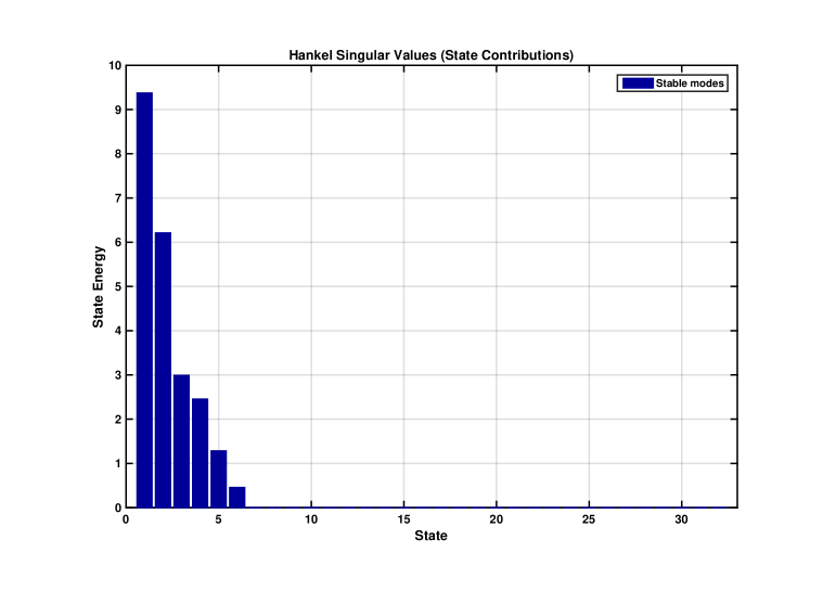
Figure 5: Hankel-singular values of the overall filter $Q(s)$.

4.8.4 afdisyn

Syntax

[Q,R,INFO] = afdisyn(SYSF,OPTIONS)

Description

afdisyn solves the approximate fault detection and isolation problem (AFDIP) (see Section 2.6.4), for a given LTI system SYSF with additive faults and a given structure matrix $S_{FDI}$ (specified via the OPTIONS structure). Two banks of stable and proper filters are computed in the $n_{b}$-dimensional cell arrays Q and R, where $n_{b}$ is the number of specifications contained in $S_{FDI}$ (i.e., the number of rows of the structure matrix $S_{FDI}$). Q{i} contains the $i$-th fault detection filter (12) in the overall solution (11) of the AFDIP and R{i} contains its internal form.

Input data

SYSF is a LTI system in the state-space form

$$E\lambda x(t) =Ax(t)+B_{u}u(t)+B_{d}d(t)+B_{f}f(t)+B_{w}w(t),$$ (161)

$$y(t) =Cx(t)+D_{u}u(t)+D_{d}d(t)+D_{f}f(t)+D_{w}w(t),$$

where any of the inputs components $u(t)$, $d(t)$, $f(t)$, or $w(t)$ can be void. For the system SYSF, the input groups for $u(t)$, $d(t)$, $f(t)$, and $w(t)$ have the standard names ’controls’, ’disturbances’, ’faults’, and ’noise’, respectively.

OPTIONS is a MATLAB structure used to specify various synthesis options and has the following fields:

OPTIONS fields	Description
SFDI	the desired structure matrix $S_{FDI}$ with $n_{b}$ rows to solve the AFDIP (Default: [1...1], i.e., solve an approximate fault detection problem)
tol	relative tolerance for rank computations (Default: internally computed)
tolmin	absolute tolerance for observability tests (Default: internally computed)
FDTol	threshold for fault detectability checks (Default: 0.0001)
FDGainTol	threshold for strong fault detectability checks (Default: 0.01)
rdim	vector, whose $i$-th component $q_{i}$, specifies the desired number of residual outputs for the $i$-th component filters Q{$i$} and R{$i$}; if OPTIONS.rdim is a scalar $q$, then a vector with all components $q_{i}=q$ is assumed.
	(Default: [ ], in which case $q_{i}=q_{i,1}+q_{i,2}$, with $q_{i,1}$ and $q_{i,2}$ selected taking into account $r_{w}^{(i)}$, the rank of the transfer function matrix from the noise input to the reduced system output employed to determine Q{$i$}, as follows: if OPTIONS.HDesign{$i$} is empty, then     $q_{i,1}=\min\big{(}1,r_{w}^{(i)}\big{)}$, if OPTIONS.minimal = true, or     $q_{i,1}=r_{w}^{(i)}$ if OPTIONS.minimal = false; if OPTIONS.HDesign{$i$} is nonempty, then $q_{i,1}$ is the row dimension of the design matrix contained in OPTIONS.HDesign{$i$}; if OPTIONS.HDesign2{$i$} is empty, then     $q_{i,2}=1-\min\big{(}1,r_{w}^{(i)}\big{)}$, if OPTIONS.minimal = true, or     $q_{i,2}$ is set to its maximum achievable value,           if OPTIONS.minimal = false; if OPTIONS.HDesign2{$i$} is nonempty, then $q_{i,2}$ is the row dimension of the design matrix contained in OPTIONS.HDesign2{$i$}.)
FDFreq	vector of real frequency values for strong detectability checks (Default: [ ])
smarg	stability margin for the poles of the component filters Q{$i$} and R{$i$}
	(Default: -sqrt(eps) for a continuous-time system SYSF;
	1-sqrt(eps) for a discrete-time system SYSF).
sdeg	prescribed stability degree for the poles of the component filters Q{$i$} and R{$i$}
	(Default: $-0.05$ for a continuous-time system SYSF;
	$0.95$ for a discrete-time system SYSF).
poles	complex vector containing a complex conjugate set of desired poles (within the stability domain) to be assigned for the component filters Q{$i$} and R{$i$} (Default: [ ])
nullspace	option to use a specific proper nullspace basis to be employed at the initial reduction step
	true – use a minimal proper basis (default); false – use a full-order observer based basis (see Method). Note: This option can only be used if no disturbance inputs are present in (161) and $E$ is invertible.
simple	option to employ simple proper bases for the synthesis of the component filters Q{$i$} and R{$i$}
	true – use simple bases;
	false – use non-simple bases (default)
minimal	option to perform least order synthesis of the component filters
	true – perform least order synthesis (default);
	false – perform full order synthesis
exact	option to perform exact filter synthesis
	true – perform exact synthesis (i.e., no optimization performed);
	false – perform approximate synthesis (default).
freq	complex frequency value to be employed to check the full row rank admissibility conditions within the function afdsyn (see Method for afdsyn) (Default:[ ], i.e., a randomly generated frequency).
tcond	maximum alowed condition number of the employed non-orthogonal transformations (Default: $10^{4}$).
FDSelect	integer vector with increasing elements containing the indices of the desired filters to be designed (Default: $[\,1,\ldots,n_{b}\,]$)
HDesign	$n_{b}$-dimensional cell array; OPTIONS.HDesign{$i$}, if not empty, is a full row rank design matrix $H_{1}^{(i)}$ employed for the synthesis of the $i$-th filter components $Q^{(1,i)}(\lambda)$ and $R^{(1,i)}(\lambda)$ (see Method) (Default: [ ])
HDesign2	$n_{b}$-dimensional cell array; OPTIONS.HDesign2{$i$}, if not empty, is a full row rank design matrix $H_{2}^{(i)}$ employed for the synthesis of the $i$-th filter components $Q^{(2,i)}(\lambda)$ and $R^{(2,i)}(\lambda)$ (see Method) (Default: [ ])
gamma	upper bound on the resulting $\|R_{w}^{(i)}(\lambda)\|_{\infty}$ (see Method) (Default: 1)
epsreg	regularization parameter used in afdsyn (Default: 0.1)
sdegzer	prescribed stability degree for zeros shifting
	(Default: $-0.05$ for a continuous-time system SYSF;
	$0.95$ for a discrete-time system SYSF).
nonstd	option to handle nonstandard optimization problems used in afdsyn:
	1 – use the quasi-co-outer–co-inner factorization (default);
	2 – use the modified co-outer–co-inner factorization with the
	regularization parameter OPTIONS.epsreg;
	3 – use the Wiener-Hopf type co-outer–co-inner factorization.
	4 – use the Wiener-Hopf type co-outer-co-inner factorization with
	zero shifting of the non-minimum phase factor using the
	stabilization parameter OPTIONS.sdegzer
	5 – use the Wiener-Hopf type co-outer-co-inner factorization with
	the regularization of the non-minimum phase factor using the
	regularization parameter OPTIONS.epsreg

Output data

Q is an $n_{b}$-dimensional cell array, with Q{$i$} containing the resulting $i$-th filter in a standard state-space representation

$$\lambda x_{Q}^{(i)}(t) =A_{Q}^{(i)}x_{Q}^{(i)}(t)+B_{Q_{y}}^{(i)}y(t)+B_{Q_{u}}^{(i)}u(t),$$

$$r^{(i)}(t) =C_{Q}^{(i)}x_{Q}^{(i)}(t)+D_{Q_{y}}^{(i)}y(t)+D_{Q_{u}}^{(i)}u(t),$$

where the residual signal $r^{(i)}(t)$ is a $q_{i}$-dimensional vector. For each system object Q{$i$}, two input groups ’outputs’ and ’controls’ are defined for $y(t)$ and $u(t)$, respectively, and the output group ’residuals’ is defined for the residual signal $r^{(i)}(t)$. Q{$i$} is empty if the index $i$ is not selected in OPTIONS.FDSelect.

R is an $n_{b}$-dimensional cell array, with R{$i$} containing the resulting internal form of the $i$-th filter in a standard state-space representation

$$\lambda x_{R}^{(i)}(t) =A_{Q}^{(i)}x_{R}^{(i)}(t)+B_{R_{f}}^{(i)}f(t)+B_{R_{w}}^{(i)}w(t),$$

$$r^{(i)}(t) =C_{Q}^{(i)}x_{R}^{(i)}(t)+D_{R_{f}}^{(i)}f(t)+D_{R_{w}}^{(i)}w(t).$$

The input groups ’faults’ and ’noise’ are defined for $f(t)$, and $w(t)$, respectively, and the output group ’residuals’ is defined for the residual signal $r^{(i)}(t)$. Note that the realizations of Q{$i$} and R{$i$} share the matrices $A_{Q}^{(i)}$ and $C_{Q}^{(i)}$. R{$i$} is empty if the index $i$ is not selected in OPTIONS.FDSelect.

INFO is a MATLAB structure containing additional information as follows:

INFO fields	Description
tcond	$n_{b}$-dimensional vector; INFO.tcond$(i)$ contains the maximum of the condition numbers of the employed non-orthogonal transformation matrices to determine the $i$-th filter component Q{$i$}; a warning is issued if any INFO.tcond$(i)$ $\geq$ OPTIONS.tcond.
HDesign	$n_{b}$-dimensional cell array; INFO.HDesign{$i$} is the $i$-th design matrix actually employed for the synthesis of the filter component $Q_{1}^{(i)}$ of the $i$-th fault detection filter Q{$i$} (see Method). INFO.HDesign{$i$} is empty if the index $i$ is not selected in OPTIONS.FDSelect.
HDesign2	$n_{b}$-dimensional cell array; INFO.HDesign2{$i$} is the $i$-th design matrix actually employed for the synthesis of the filter component $Q_{2}^{(i)}$ of the $i$-th fault detection filter Q{$i$} (see Method). INFO.HDesign2{$i$} is empty if the index $i$ is not selected in OPTIONS.FDSelect.
freq	complex frequency value employed to check the full row rank admissibility conditions within the function afdsyn
gap	$n_{b}$-dimensional cell array; INFO.gap$(i)$ contains the $i$-th gap $\eta_{i}$ resulted by calling afdsyn to determine Q{$i$} (see Method).

Method

The Procedure AFDI from [16, Sect. 5.4] is implemented, which relies on the optimization-based synthesis method proposed in [9]. Each filter $Q^{(i)}(\lambda)$ and its internal form $R^{(i)}(\lambda)$, are determined by solving a suitably formulated AFDP for a reduced system without control inputs, and with redefined disturbance and fault inputs. For this purpose, the function afdisyn calls internally the function afdsyn to solve a suitably formulated AFDP for each specification (i.e., row) contained in the structure matrix $S_{FDI}$.

If the faulty system SYSF has the input-output form

$${\mathbf{y}}(\lambda)=G_{u}(\lambda){\mathbf{u}}(\lambda)+G_{d}(\lambda){\mathbf{d}}(\lambda)+G_{f}(\lambda){\mathbf{f}}(\lambda)+G_{w}(\lambda){\mathbf{w}}(\lambda)$$ (162)

and the $i$-th fault detection filter $Q^{(i)}(\lambda)$ contained in Q{$i$} has the input-output form

$${\mathbf{r}}^{(i)}(\lambda)=Q^{(i)}(\lambda)\left[\begin{array}[]{c}{\mathbf{y}}(\lambda)\\ {\mathbf{u}}(\lambda)\end{array}\right]\,,$$ (163)

then, taking into account the decoupling conditions (19), the resulting internal form of the $i$-th fault detection filter $R^{(i)}(\lambda)$, contained in R{$i$}, is

$${\mathbf{r}}^{(i)}(\lambda)=R^{(i)}(\lambda){\left[\begin{array}[]{c}{\mathbf{f}}(\lambda)\\ {\mathbf{w}}(\lambda)\end{array}\right]}=R_{f}^{(i)}(\lambda){\mathbf{f}}(\lambda)+R_{w}^{(i)}(\lambda){\mathbf{w}}(\lambda)\,,$$ (164)

with $R^{(i)}(\lambda)=[\,R_{f}^{(i)}(\lambda)\;R_{w}^{(i)}(\lambda)\,]$ defined as

$$\left[\begin{array}[]{c|c}R_{f}^{(i)}(\lambda)&R_{w}^{(i)}(\lambda)\end{array}\right]:={Q^{(i)}(\lambda)\left[\begin{array}[]{c|c}G_{f}(\lambda)&G_{w}(\lambda)\\ 0&0\end{array}\right]}\,.$$ (165)

When determining $Q^{(i)}(\lambda)$ it is first attempted to solve the strict AFDIP (26), such that the structure vector corresponding to the zero and nonzero columns of $R_{f}^{(i)}(\lambda)$ is equal to the $i$-th row of the specified $S_{FDI}$. If this is not achievable, then the soft AFDIP (25) is attempted to be solved.

The achieved gap $\eta_{i}$ is computed as $\eta_{i}=\big{\|}\overline{R}_{f}^{(i)}(\lambda)\big{\|}_{\infty-}/\big{\|}\big{[}\widetilde{R}_{f}^{(i)}(\lambda)\;R_{w}^{(i)}(\lambda)\big{]}\big{\|}_{\infty}$, where $\overline{R}_{f}^{(i)}(\lambda)$ is formed from the columns of $R_{f}^{(i)}(\lambda)$ corresponding to nonzero entries in the $i$-th row of $S_{FDI}$ and $\widetilde{R}_{f}^{(i)}(\lambda)$ is formed from the columns of $R_{f}^{(i)}(\lambda)$ corresponding to zero entries in the $i$-th row of $S_{FDI}$. If OPTIONS.FDFreq is nonempty, then $\big{\|}\overline{R}_{f}^{(i)}(\lambda)\big{\|}_{\infty-}$ is only evaluated over the frequency values contained in OPTIONS.FDFreq. The achieved gaps are returned in INFO.gap.

Each filter $Q^{(i)}(\lambda)$ is determined in the product form

$$Q^{(i)}(\lambda)=\overline{Q}_{1}^{(i)}(\lambda)Q_{1}(\lambda),$$ (166)

where the factors are determined as follows:

• $Q_{1}(\lambda)=N_{l}(\lambda)$, with $N_{l}(\lambda)$ a $\big{(}p-r_{d}\big{)}\times(p+m_{u})$ proper rational left nullspace basis satisfying $N_{l}(\lambda)\left[\begin{smallmatrix}G_{u}(\lambda)&G_{d}(\lambda)\\ I_{m_{u}}&0\end{smallmatrix}\right]=0$, with $r_{d}:=\text{rank}\,G_{d}(\lambda)$;

• $\overline{Q}_{1}^{(i)}(\lambda)$ is the solution of a suitably formulated AFDP to achieve the specification contained in the $i$-th row of $S_{FDI}$. The function afdsyn is called for this purpose and internally uses the design matrices $H_{1}^{(i)}$, which can be specified in OPTIONS.HDesign{$i$}, and $H_{2}^{(i)}$, which can be specified in OPTIONS.HDesign2{$i$} (see Method for afdsyn). The actually employed design matrices are returned in INFO.HDesign{$i$} and INFO.HDesign2{$i$}, respectively.

Each factor $\overline{Q}_{1}^{(i)}(\lambda)$ is determined in the partitioned form

$$\overline{Q}_{1}^{(i)}(\lambda)=\left[\begin{array}[]{cc}\overline{Q}_{1}^{(i,1)}(\lambda)\\ \overline{Q}_{1}^{(i,2)}(\lambda)\end{array}\right],$$

where the computation of individual factors $\overline{Q}_{1}^{(i,1)}(\lambda)$ and $\overline{Q}_{1}^{(i,2)}(\lambda)$ depends on the user’s options (see Method for the function afdsyn). In what follows, we only discuss shortly the computation of $Q_{1}(\lambda)$, performed only once as an initial reduction step.

If OPTIONS.nullspace = true or $m_{d}>0$ or $E$ is singular, then $N_{l}(\lambda)$ is determined as a minimal proper nullspace basis. In this case, only orthogonal transformations are performed at this computational step.

If OPTIONS.nullspace = false, $m_{d}=0$ and $E$ is invertible, then $N_{l}(\lambda)=[\,I_{p}\;-G_{u}(\lambda)\,]$ is used, which corresponds to a full-order Luenberger observer. This option involves no numerical computations.

Example

Example 11.

This is Example 5.3 from the book [16], with the disturbances redefined as noise inputs and by adding a sensor fault for the first output measurement. The TFMs of the system are:

$$G_{u}(s)={\left[\begin{array}[]{c}\displaystyle\frac{s+1}{s+2}\\ \\[-5.69054pt] \displaystyle\frac{s+2}{s+3}\end{array}\right],\quad G_{d}(s)=0,\quad G_{f}(s)=[\,G_{u}(s)\;I\,],\quad G_{w}(s)=\left[\begin{array}[]{c}\displaystyle\frac{s-1}{s+2}\\ \\[-5.69054pt] 0\end{array}\right]},$$

where the fault input $f_{1}$ corresponds to an additive actuator fault, while the fault inputs $f_{2}$ and $f_{3}$ describe additive sensor faults in the outputs $y_{1}$ and $y_{2}$, respectively. The transfer function matrix $G_{w}(s)$ is non-minimum phase, having an unstable zero at 1. Interestingly, the EFDIP formulated with $G_{d}(s)=G_{w}(s)$ is not solvable.

The maximal achievable structure matrix (for the EFDIP) is

$$S_{max}=\left[\begin{array}[]{ccc}1&1&1\\ 0&1&1\\ 1&0&1\\ 1&1&0\end{array}\right]\,.$$

We assume that no simultaneous faults occur, and thus we can target to solve an AFDIP for the structure matrix

$$S_{FDI}=\left[\begin{array}[]{ccc}0&1&1\\ 1&0&1\\ 1&1&0\end{array}\right]\,,$$

where the columns of $S_{FDI}$ codify the desired fault signatures.

We want to design a bank of three detection filters $Q^{(i)}(s)$, $i=1,2,3$ which fulfill for each $i$:

• the decoupling condition: $Q^{(i)}(s)\left[\begin{smallmatrix}G_{u}(s)&G_{d}(s)\\ I_{m_{u}}&0\end{smallmatrix}\right]=0$;

• the fault isolability condition: $S_{R_{f}^{(i)}}$ is equal to the $i$-th row of $S_{FDI}$;

• the maximization of the noise attenuation gap: $\eta_{i}:=\|\overline{R}_{f}^{(i)}(s)\|_{\infty-}/\|R_{w}^{(i)}(s)\|_{\infty}=\max$, where $\overline{R}_{f}^{(i)}(s)$ is formed from the columns of $R_{f}^{(i)}(s)$ corresponding to nonzero entries in the $i$-th row of $S_{FDI}$.

The results computed with the following script are:
– $\eta_{1}=1.5$ with

$$Q^{(1)}(s)={\left[\begin{array}[]{ccc}\displaystyle\frac{s+2}{s+1}&-\displaystyle\frac{s+3}{s+2}&0\end{array}\right],\quad R_{f}^{(1)}(s)=\left[\begin{array}[]{ccc}0&\displaystyle\frac{s+2}{s+1}&-\displaystyle\frac{s+3}{s+2}\end{array}\right]},\quad R_{w}^{(1)}(s)=\displaystyle\frac{s-1}{s+1}\;;$$

– $\eta_{2}=\infty$ with

$$Q^{(2)}(s)={\left[\begin{array}[]{ccc}0&1&-\displaystyle\frac{s+2}{s+3}\end{array}\right],\quad R_{f}^{(2)}(s)=\left[\begin{array}[]{ccc}\displaystyle\frac{s+2}{s+3}&0&1\end{array}\right]},\quad R_{w}^{(2)}(s)=0\;;$$

– $\eta_{3}=1$ with

$$Q^{(3)}(s)={\left[\begin{array}[]{ccc}\displaystyle\frac{s+2}{s+1}&0&-1\end{array}\right],\quad R_{f}^{(3)}(s)=\left[\begin{array}[]{ccc}1&\displaystyle\frac{s+2}{s+1}&0\end{array}\right]},\quad R_{w}^{(3)}(s)=\displaystyle\frac{s-1}{s+1}\;.$$

% Example - Solution of an approximate fault detection problem (AFDIP)

% Example 5.3 of (V,2017) (modified)
s = tf(’s’); % define the Laplace variable s
mu = 1; mw = 1; p = 2; mf = mu+p; % set dimensions
Gu = [(s+1)/(s+2); (s+2)/(s+3)];  % enter Gu(s)
Gw = [(s-1)/(s+2); 0];            % enter Gw(s)

% build the model with additive faults having Gf(s) = [Gu(s) eye(p)];
sysf = fdimodset(ss([Gu Gw]),struct(’c’,1,’f’,1,’fs’,1:2,’n’,2));

% select SFDI
S = fdigenspec(sysf); SFDI = S(sum(S,2)==2,:)
nb = size(SFDI,1);

% perform synthesis with AFDISYN
options = struct(’tol’,1.e-7,’smarg’,-3,...
                 ’sdeg’,-3,’SFDI’,SFDI);
[Q,R,info] = afdisyn(sysf,options);

% display the implementation form Q{i}(s) and the internal forms
% Rf{i}(s) and Rw{i}(s) of the resulting fault detection filters
minreal(tf(Q{1})), minreal(tf(R{1}(:,’faults’))), minreal(tf(R{1}(:,’noise’)))
minreal(tf(Q{2})), minreal(tf(R{2}(:,’faults’))), tf(R{2}(:,’noise’))
minreal(tf(Q{3})), minreal(tf(R{3}(:,’faults’))), tf(R{3}(:,’noise’))

% check the resulting gaps
format short e
info.gap
gap = fdif2ngap(R,[],SFDI)

% simulate step responses from fault and noise inputs
inpnames = {’f_1’,’f_2’,’f_3’,’w’};
outnames = {’r_1’,’r_2’,’r_3’};
Rtot = vertcat(R{:});
set(Rtot,’InputName’,inpnames,’OutputName’,outnames);
step(Rtot); ylabel(’Residuals’)
title(’Step responses from fault and noise inputs’)

4.8.5 emmsyn

Syntax

[Q,R,INFO] = emmsyn(SYSF,SYSR,OPTIONS)

Description

emmsyn solves the exact model matching problem (EMMP) (as formulated in the more general form (29) in Remark 7; see Section 2.6.5), for a given LTI system SYSF with additive faults and a given stable reference filter SYSR. Two stable and proper filters, Q and R, are computed, where Q contains the fault detection and isolation filter representing the solution of the EMMP, and R contains its internal form.

Input data

SYSF is a LTI system in the state-space form

$$E\lambda x(t) =Ax(t)+B_{u}u(t)+B_{d}d(t)+B_{f}f(t)+B_{w}w(t),$$ (167)

$$y(t) =Cx(t)+D_{u}u(t)+D_{d}d(t)+D_{f}f(t)+D_{w}w(t),$$

where any of the inputs components $u(t)$, $d(t)$, $f(t)$, or $w(t)$ can be void. For the system SYSF, the input groups for $u(t)$, $d(t)$, $f(t)$, and $w(t)$ have the standard names ’controls’, ’disturbances’, ’faults’, and ’noise’, respectively.

SYSR is a proper and stable LTI system in the state-space form

$$\lambda x_{r}(t) =A_{r}x_{r}(t)+B_{ru}u(t)+B_{rd}d(t)+B_{rf}f(t)+B_{rw}w(t),$$ (168)

$$y_{r}(t) =C_{r}x_{r}(t)+D_{ru}u(t)+D_{rd}d(t)+D_{rf}f(t)+D_{rw}w(t),$$

where the reference model output $ry_{(}t)$ is a $q$-dimensional vector and any of the inputs components $u(t)$, $d(t)$, $f(t)$, or $w(t)$ can be void. For the system SYSR, the input groups for $u(t)$, $d(t)$, $f(t)$, and $w(t)$ have the standard names ’controls’, ’disturbances’, ’faults’, and ’noise’, respectively.

OPTIONS is a MATLAB structure used to specify various synthesis options and has the following fields:

OPTIONS fields	Description
tol	relative tolerance for rank computations (Default: internally computed)
tolmin	absolute tolerance for observability tests (Default: internally computed)
smarg	stability margin for the poles of the filters Q and R
	(Default: -sqrt(eps) for a continuous-time system SYSF;
	1-sqrt(eps) for a discrete-time system SYSF).
sdeg	prescribed stability degree for the poles of the filters Q and R
	(Default: $-0.05$ for a continuous-time system SYSF;
	$0.95$ for a discrete-time system SYSF).
poles	complex vector containing a complex conjugate set of desired poles (within the stability domain) to be assigned for the filters Q and R (Default: [ ])
simple	option to employ a simple proper basis for synthesis
	true – use a simple basis;
	false – use a non-simple basis (default)
minimal	option to perform least order synthesis of the filter Q
	true – perform least order synthesis (default);
	false – perform full order synthesis
regmin	option to perform regularization selecting a least order left annihilator
	true – perform least order selection (default);
	false – no least order selection performed
tcond	maximum allowed condition number of the employed non-orthogonal transformations (Default: $10^{4}$).
normalize	option for the normalization of the diagonal elements of the updating matrix $M(\lambda)$:
	’gain’ – scale with the gains of the zero-pole-gain representation (default) ’dcgain’ – scale with the DC-gains ’infnorm’ – scale with the values of infinity-norms
freq	complex frequency value to be employed to check the left-invertibility-based solvability condition (see Method) (Default:[ ], i.e., a randomly generated frequency).
HDesign	full row rank design matrix $H$ employed for the synthesis of the filter Q (see Method) (Default: [ ])
	Note. This option can be only used in conjunction with the “no least order synthesis” option: OPTIONS.minimal = false.

Output data

Q is the resulting fault detection filter in a standard state-space representation

$$\lambda x_{Q}(t) =A_{Q}x_{Q}(t)+B_{Q_{y}}y(t)+B_{Q_{u}}u(t),$$ (169)

$$r(t) =C_{Q}x_{Q}(t)+D_{Q_{y}}y(t)+D_{Q_{u}}u(t),$$

where the residual signal $r(t)$ is a $q$-dimensional vector. For the system object Q, two input groups ’outputs’ and ’controls’ are defined for $y(t)$ and $u(t)$, respectively, and the output group ’residuals’ is defined for the residual signal $r(t)$.

R is the resulting internal form of the fault detection filter in a standard state-space representation

$$\lambda x_{R}(t) =A_{R}x_{R}(t)+B_{R_{u}}u(t)+B_{R_{d}}d(t)+B_{R_{f}}f(t)+B_{R_{w}}w(t),$$ (170)

$$r(t) =C_{R}x_{R}(t)+D_{R_{u}}u(t)+D_{R_{d}}d(t)+D_{R_{f}}f(t)+D_{R_{w}}w(t)$$

with the same input groups defined as for SYSR and the output group ’residuals’ defined for the residual signal $r(t)$.

INFO is a MATLAB structure containing additional information as follows:

INFO fields	Description
tcond	the maximum of the condition numbers of the employed non-orthogonal transformation matrices; a warning is issued if INFO.tcond $\geq$ OPTIONS.tcond.
degs	the left Kronecker indices of $G(\lambda):=\left[\begin{smallmatrix}G_{u}(\lambda)&G_{u}(\lambda)\\ I&0\end{smallmatrix}\right]$ (see Method); also the increasingly ordered degrees of a left minimal polynomial nullspace basis of $G(\lambda)$; (INFO.degs = [ ] if no explicit left nullspace basis is computed)
M	state-space realization of the employed updating matrix $M(\lambda)$ (see Method)
freq	complex frequency value employed to check the left invertibility condition; INFO.freq = [ ] if no frequency-based left invertibility check was performed.
HDesign	design matrix $H$ employed for the synthesis of the fault detection filter; INFO.HDesign = [ ] if no design matrix was explicitly involved in the filter synthesis.

Method

Extensions of the Procedure EMM and Procedure EMMS from [16, Sect. 5.6] are implemented in the function emmsyn. The Procedure EMM relies on the model-matching synthesis method proposed in [6], while Procedure EMMS uses the inversion-based method proposed in [14] in conjunction with the nullspace method. The Procedure EMM is employed to solve the general EMMP (see below), while Procedure EMMS is employed to solve the more particular (but more practice relevant) strong exact fault detection and isolation problem (strong EFDIP).

Assume that the system SYSF has the input-output form

$${\mathbf{y}}(\lambda)=G_{u}(\lambda){\mathbf{u}}(\lambda)+G_{d}(\lambda){\mathbf{d}}(\lambda)+G_{f}(\lambda){\mathbf{f}}(\lambda)+G_{w}(\lambda){\mathbf{w}}(\lambda)$$ (171)

and the reference model SYSR has the input-output form

$${\mathbf{y}}_{r}(\lambda)=M_{ru}(\lambda){\mathbf{u}}(\lambda)+M_{rd}(\lambda){\mathbf{d}}(\lambda)+M_{rf}(\lambda){\mathbf{f}}(\lambda)+M_{rw}(\lambda){\mathbf{w}}(\lambda),$$ (172)

where the vectors $y$, $u$, $d$, $f$, $w$ and $y_{r}$ have dimensions $p$, $m_{u}$, $m_{d}$, $m_{f}$, $m_{w}$ and $q$, respectively. The resulting fault detection filter in (169) has the input-output form

$${\mathbf{r}}(\lambda)=Q(\lambda)\left[\begin{array}[]{c}{\mathbf{y}}(\lambda)\\ {\mathbf{u}}(\lambda)\end{array}\right],$$ (173)

where the resulting dimension of the residual vector $r$ is $q$.

The function emmsyn determines $Q(\lambda)$ by solving the general exact model-matching problem

$${Q(\lambda)\left[\begin{array}[]{c|c|c|c}G_{u}(\lambda)&G_{d}(\lambda)&G_{f}(\lambda)&G_{w}(\lambda)\\ I_{m_{u}}&0&0&0\end{array}\right]}=M(\lambda)\big{[}\,M_{ru}(\lambda)\mid M_{rd}(\lambda)\mid M_{rf}(\lambda)\mid M_{rw}(\lambda)\,\big{]}\,,$$ (174)

where $M(\lambda)$ is a stable, diagonal and invertible transfer function matrix chosen such that the resulting solution $Q(\lambda)$ of the linear rational matrix equation (174) is stable and proper. The resulting internal form $R(\lambda)$, contained in R, is computed as

$$R(\lambda):=\big{[}\,R_{u}(\lambda)\!\mid\!R_{d}(\lambda)\!\mid\!R_{f}(\lambda)\!\mid\!R_{w}(\lambda)\,\big{]}:=M(\lambda)\big{[}\,M_{ru}(\lambda)\!\mid\!M_{rd}(\lambda)\!\mid\!M_{rf}(\lambda)\!\mid\!M_{rw}(\lambda)\,\big{]}.$$ (175)

Two cases are separately addressed, depending on the presence or absence of $M_{rw}(\lambda)$ in the reference model (172).

In the first case, when $M_{rw}(\lambda)$ is present, the general EMMP (174) is solved, with $M_{ru}(\lambda)$, or $M_{rd}(\lambda)$, or both of them, explicitly set to zero if not present in the reference model. In the second case, when $M_{rw}(\lambda)$ is not present, then $Q(\lambda)$ is determined by solving the EMMP

$${Q(\lambda)\left[\begin{array}[]{c|c|c}G_{u}(\lambda)&G_{d}(\lambda)&G_{f}(\lambda)\\ I_{m_{u}}&0&0\end{array}\right]}=M(\lambda)\big{[}\,M_{ru}(\lambda)\mid M_{rd}(\lambda)\mid M_{rf}(\lambda)\,\big{]}$$ (176)

with $M_{ru}(\lambda)$, or $M_{rd}(\lambda)$, or both of them, explicitly set to zero if not present in the reference model. In this case, if $G_{w}(\lambda)$ is present in the plant model (171), then $R_{w}(\lambda)$ is explicitly computed as

$$R_{w}(\lambda)=Q(\lambda)\left[\begin{array}[]{c}G_{w}(\lambda)\\ 0\end{array}\right].$$

The particular EMMP formulated in Section 2.6.5 corresponds to solve the EMMP (176) with $M_{ru}(\lambda)=0$, $M_{rd}(\lambda)=0$.

If OPTIONS.minimal = true, then a least order solution $Q(\lambda)$ is determined in the form $Q(\lambda)=Q_{2}(\lambda)Q_{1}(\lambda)$, where $Q_{1}(\lambda)$ is a least McMillan degree solution of the linear rational matrix equation

$${Q_{1}(\lambda)\left[\begin{array}[]{c|c|c|c}G_{u}(\lambda)&G_{d}(\lambda)&G_{f}(\lambda)&G_{w}(\lambda)\\ I_{m_{u}}&0&0&0\end{array}\right]}=\big{[}\,M_{ru}(\lambda)\mid M_{rd}(\lambda)\mid M_{rf}(\lambda)\mid M_{rw}(\lambda)\,\big{]}$$ (177)

and the diagonal updating factor $Q_{2}(\lambda):=M(\lambda)$ is determined to ensure that $Q(\lambda)$ is proper and stable.

If OPTIONS.minimal = false and either $M_{ru}(\lambda)$ or $M_{rd}(\lambda)$, or both, are present in the reference model (172), then $Q(\lambda)$ is determined in the form $Q(\lambda)=Q_{2}(\lambda)Q_{1}(\lambda)$, where $Q_{1}(\lambda)$ is a particular solution of the linear rational equation (177) and the diagonal updating factor $Q_{2}(\lambda):=M(\lambda)$ is determined to ensure that $Q(\lambda)$ is proper and stable.

If OPTIONS.minimal = false and if both $M_{ru}(\lambda)$ and $M_{rd}(\lambda)$ are absent in the reference model (172), then the nullspace method is employed as the first computational step of solving the EMMP (see Procedure EMM in [16]). The strong EFDIP arises if additionally $M_{rf}(\lambda)$ is diagonal and invertible, in which case, an extension of the Procedure EMMS in [16] is employed. In fact, this procedure works for arbitrary invertible $M_{rf}(\lambda)$ and this case was considered for the implementation of emmsyn. The solution of a fault estimation problem can be targeted by choosing $M_{rf}(\lambda)=I_{m_{f}}$ and checking that the resulting $M(\lambda)=I_{m_{f}}$. Recall that $M(\lambda)$ is provided in INFO.M. In what follows, we give some details of the implemented synthesis approach employed if $M_{ru}(\lambda)$, $M_{rd}(\lambda)$ and $M_{rw}(\lambda)$ are not present in reference model.

If OPTIONS.regmin = false, then $Q(\lambda)$ is determined in the form

$$Q(\lambda)=M(\lambda)Q_{2}(\lambda)HN_{l}(\lambda),$$

where: $N_{l}(\lambda)$ is a $\big{(}p-r_{d}\big{)}\times(p+m_{u})$ rational left nullspace basis satisfying

$$N_{l}(\lambda)\left[\begin{array}[]{cc}G_{u}(\lambda)&G_{d}(\lambda)\\ I_{m_{u}}&0\end{array}\right]=0,$$

with $r_{d}:=\text{rank}\,G_{d}(\lambda)$; $H$ is a suitable full row rank design matrix used to build $q$ linear combinations of the $p-r_{d}$ left nullspace basis vectors ($q$ is the number of outputs of SYSR); $Q_{2}(\lambda)$ is the solution of $Q_{2}(\lambda)H\overline{G}_{f}(\lambda)=M_{rf}(\lambda)$, where

$$\overline{G}_{f}(\lambda)=N_{l}(\lambda)\left[\begin{array}[]{c}G_{f}(\lambda)\\ 0\end{array}\right];$$

and $M(\lambda)$ is a stable invertible transfer function matrix determined such that $Q(\lambda)$ and the corresponding $\widetilde{R}(\lambda)$ in (175) have desired dynamics (specified via OPTIONS.sdeg and OPTIONS.poles). The internal form of the filter $Q(\lambda)$ is obtained as

$$R(\lambda)=M(\lambda)Q_{2}(\lambda)H\overline{G}(\lambda),$$

where

$$\overline{G}(\lambda):=\big{[}\,\overline{G}_{f}(\lambda)\mid\overline{G}_{w}(\lambda)\,\big{]}=N_{l}(\lambda)\left[\begin{array}[]{c|c}G_{f}(\lambda)&G_{w}(\lambda)\\ 0&0\end{array}\right]\,.$$

The solvability condition of the strong EFDIP is verified by checking the left invertibility condition

$$\mathop{\mathrm{rank}}H\overline{G}_{f}(\lambda_{s})=m_{f},$$ (178)

where $\lambda_{s}$ is a suitable frequency value, which can be specified via the OPTIONS.freq. The design parameter matrix $H$ is set as follows: if OPTIONS.HDesign is nonempty, then $H=\texttt{OPTIONS.HDesign}$; if OPTIONS.HDesign = [ ], then $H=I_{p-r_{d}}$, if $q=p-r_{d}$, or $H$ is a randomly generated $q\times\big{(}p-r_{d}\big{)}$ real matrix, if $q<p-r_{d}$. If OPTIONS.simple = true, then $N_{l}(\lambda)$ is determined as a simple rational basis. The orders of the basis vectors are provided in INFO.degs. These are also the degrees of the basis vectors of an equivalent polynomial nullspace basis.

If OPTIONS.regmin = true, then $[\,Q(\lambda)\;R_{f}(\lambda)\,]$ has the least McMillan degree, with $Q(\lambda)$ having $q$ outputs. $Q(\lambda)$ and $R_{f}(\lambda)$ are determined in the form

$$[\,Q(\lambda)\mid R_{f}(\lambda)\,]=M(\lambda)Q_{2}(\lambda)\big{[}\,\overline{Q}(\lambda)\mid\overline{R}_{f}(\lambda)\,\big{]}\,,$$

where

$$\big{[}\,\overline{Q}(\lambda)\mid\overline{R}_{f}(\lambda)\,\big{]}=H\big{[}\,N_{l}(\lambda)\mid\overline{G}_{f}(\lambda)\,\big{]}+Y(\lambda)\big{[}\,N_{l}(\lambda)\mid\overline{G}_{f}(\lambda)\,\big{]}$$

with $[\,\overline{Q}(\lambda)\;\overline{R}_{f}(\lambda)\,]$ and $Y(\lambda)$ the least order solution of a left minimal cover problem [15]; $Q_{2}(\lambda)$ is the solution of $Q_{2}(\lambda)\overline{R}_{f}(\lambda)=M_{rf}(\lambda)$; and $M(\lambda)$ is a stable invertible transfer function matrix determined such that $[\,Q(\lambda)\;R(\lambda)\,]$ has a desired dynamics. If OPTIONS.HDesign is nonempty, then $H=\texttt{OPTIONS.HDesign}$, and if OPTIONS.HDesign = [ ], then a suitable randomly generated $H$ is employed, which fulfills the left invertibility condition (178).

The actually employed design matrix $H$ is provided in INFO.HDesign, and INFO.HDesign = [ ] if the solution of the EMMP is obtained by directly solving (174).

Examples

Example 12.

This is Example 5.12 from the book [16] and was used in Example 9, to solve an EFDIP for a system with triplex sensor redundancy. To solve the same problem by solving an EMMP, we use the resulting $R_{f}(s)$ to define the reference model

$$M_{rf}(s):=R_{f}(s)=\left[\begin{array}[]{rrr}0&1&-1\\ -1&0&1\\ 1&-1&0\end{array}\right]\,.$$

The resulting least order filter $Q(s)$, determined by employing emmsyn with Procedure EMM, has the generic form

$$Q(s)=\left[\begin{array}[]{rrrccc}0&1&-1&0&\cdots&0\\ -1&0&1&0&\cdots&0\\ 1&-1&0&0&\cdots&0\end{array}\right]\,.$$

% Example - Solution of an EMMP

p = 3; mf = 3;   % enter output and fault vector dimensions
% generate random dimensions for system order and input vectors
rng(’default’)
nu = floor(1+4*rand); mu = floor(1+4*rand);
nd = floor(1+4*rand); md = floor(1+4*rand);
% define random Gu(s) and Gd(s) with triplex sensor redundancy
% and Gf(s) = I for triplex sensor faults
Gu = ones(3,1)*rss(nu,1,mu); % enter Gu(s) in state-space form
Gd = ones(3,1)*rss(nd,1,md); % enter Gd(s) in state-space form

% build synthesis model with sensor faults
sysf = fdimodset([Gu Gd],struct(’c’,1:mu,’d’,mu+(1:md),’fs’,1:3));

% enter reference model for the TFM from faults to residual
Mr = fdimodset(ss([ 0 1 -1; -1 0 1; 1 -1 0]),struct(’f’,1:mf));

% solve an exact model-matching problem using EMMSYN
[Q,R,info] = emmsyn(sysf,Mr);

% determine achieved fault sensitivity conditions
FSCOND = fdifscond(R,0,fdisspec(Mr))

% check the synthesis: Q*Ge = M*Me and R = M*Mr, where
% Ge = [Gu Gd Gf; I 0 0] and Me = [0 0 Mr ].
Ge = [sysf; eye(mu,mu+md+mf)]; Me = [zeros(p,mu+md) Mr];
norm(gminreal(Q*Ge)-info.M*Me,inf)
norm(R-info.M*Mr,inf)

Example 13.

This is Example 5.13 from the book [16], with a continuous-time system with additive actuator faults, having the transfer-function matrices

$$G_{u}(s)=\left[\begin{array}[]{cc}\displaystyle\frac{s}{s^{2}+3\,s+2}&\displaystyle\frac{1}{s+2}\\ \\[-5.69054pt] \displaystyle\frac{s}{s+1}&0\\ \\[-5.69054pt] 0&\displaystyle\frac{1}{s+2}\end{array}\right],\quad G_{d}(s)=0,\quad G_{f}(s)=G_{u}(s),\quad G_{w}(s)=0\,.$$

We want to solve an EMMP with the reference model

$$M_{rf}(s)={\left[\begin{array}[]{cc}1&0\\ 0&1\end{array}\right]}\,,$$

which is equivalent to solve a strong EFDIP with the structure matrix

$$S_{FDI}={\left[\begin{array}[]{cc}1&0\\ 0&1\end{array}\right]}.$$

A least order stable filter $Q(s)$, with poles assigned to $-1$, has been determined by employing emmsyn with Procedure EMMS of [16] (which is employed if OPTIONS.minimal = false). The resulting $Q(s)$ is

$$Q(s)={\left[\begin{array}[]{ccccc}0&1&0&-\displaystyle\frac{s}{s+1}&0\\ 0&0&\displaystyle\frac{s+2}{s+1}&0&-\displaystyle\frac{1}{s+1}\end{array}\right]}$$

and has the McMillan degree equal to 2. The resulting updating factor is

$$M(s)=\left[\begin{array}[]{cc}\displaystyle\frac{s}{s+1}&0\\ 0&\displaystyle\frac{1}{s+1}\end{array}\right]$$

and has McMillan degree 2. The presence of the zero at $s=0$ in $R(s):=M(s)M_{r}(s)$ is unavoidable for the existence of a stable solution. It follows, that while a constant actuator fault $f_{2}$ is strongly detectable, a constant actuator fault $f_{1}$ is only detectable during transients.

% Example - Solution of a strong EFDIP as an EMMP

% define s as an improper transfer function
s = tf(’s’);
% enter Gu(s)
Gu = [s/(s^2+3*s+2) 1/(s+2);
     s/(s+1) 0;
      0 1/(s+2)];
[p,mu] = size(Gu); mf = mu;

% build model with faults
sysf = fdimodset(ss(Gu),struct(’c’,1:mu,’f’,1:mu));

% define Mr(s)
Mr = fdimodset(ss(eye(2)),struct(’f’,1:mf));

% solve a strong EFDIP using EMMSYN (for an invertible reference model)
opts_emmsyn = struct(’tol’,1.e-7,’sdeg’,-1,’minimal’,false);
[Q,R,info] = emmsyn(sysf,Mr,opts_emmsyn);

% check solution
G = [sysf;eye(mu,mu+mf)];
norm(Q*G-info.M*[zeros(mf,mu) Mr],inf)

% display results
minreal(tf(Q)), tf(info.M)

4.8.6 ammsyn

Syntax

[Q,R,INFO] = ammsyn(SYSF,SYSR,OPTIONS)

Description

ammsyn solves the approximate model matching problem (AMMP); (see Section 2.6.6), for a given LTI system SYSF with additive faults and a given stable reference filter SYSR. Two stable and proper filters, Q and R, are computed, where Q contains the fault detection and isolation filter representing the solution of the AMMP, and R contains its internal form.

Input data

SYSF is a LTI system in the state-space form

$$E\lambda x(t) =Ax(t)+B_{u}u(t)+B_{d}d(t)+B_{f}f(t)+B_{w}w(t),$$ (179)

$$y(t) =Cx(t)+D_{u}u(t)+D_{d}d(t)+D_{f}f(t)+D_{w}w(t),$$

where any of the inputs components $u(t)$, $d(t)$, $f(t)$ or $w(t)$ can be void. For the system SYSF, the input groups for $u(t)$, $d(t)$, $f(t)$, and $w(t)$ must have the standard names ’controls’, ’disturbances’, ’faults’, and ’noise’, respectively.

SYSR is a proper and stable LTI system in the state-space form

$$\lambda x_{r}(t) =A_{r}x_{r}(t)+B_{ru}u(t)+B_{rd}d(t)+B_{rf}f(t)+B_{rw}w(t),$$ (180)

$$y_{r}(t) =C_{r}x_{r}(t)+D_{ru}u(t)+D_{rd}d(t)+D_{rf}f(t)+D_{rw}w(t),$$

where the reference model output $y_{r}(t)$ is a $q$-dimensional vector and any of the inputs components $u(t)$, $d(t)$, $f(t)$, or $w(t)$ can be void. For the system SYSR, the input groups for $u(t)$, $d(t)$, $f(t)$, and $w(t)$ must have the standard names ’controls’, ’disturbances’, ’faults’, and ’noise’, respectively.

OPTIONS is a MATLAB structure used to specify various synthesis options and has the following fields:

OPTIONS fields	Description
tol	relative tolerance for rank computations (Default: internally computed)
tolmin	absolute tolerance for observability tests (Default: internally computed)
smarg	stability margin for the poles of the updating factor $M(\lambda)$ (see Method)
	(Default: -sqrt(eps) for a continuous-time system SYSF;
	1-sqrt(eps) for a discrete-time system SYSF).
sdeg	prescribed stability degree for the poles of the updating factor $M(\lambda)$ (see Method)
	(Default: $-0.05$ for a continuous-time system SYSF;
	$0.95$ for a discrete-time system SYSF).
poles	complex vector containing a complex conjugate set of desired poles (within the stability domain) to be assigned for the updating factor $M(\lambda)$ (see Method) (Default: [ ])
nullspace	option to use a specific proper nullspace basis to be employed in the nullspace-based synthesis step
	true – use a minimal proper basis (default); false – use a full-order observer based basis (see Method). Note: This option can only be used if no disturbance inputs are present in (179) and $E$ is invertible.
simple	option to employ a simple proper basis for the nullspace-based synthesis
	true – use a simple basis;
	false – use a non-simple basis (default)
mindeg	option to compute a minimum degree solution
	true – determine, if possible, a minimum order stable solution false – determine a particular stable solution which has possibly non-minimal (default).
regmin	regularization option with least order left annihilator selection
	true – perform least order selection (default);
	false – no least order selection to be performed
tcond	maximum allowed condition number of the employed non-orthogonal transformations (Default: $10^{4}$).
normalize	option for the normalization of the diagonal elements of the updating matrix $M(\lambda)$ (see Method):
	’gain’ – scale with the gains of the zero-pole-gain representation (default) ’dcgain’ – scale with the DC-gains ’infnorm’ – scale with the values of infinity-norms
freq	complex frequency value to be employed to check frequency response based (admissibility) rank conditions (see Method) (Default:[ ], i.e., a randomly generated frequency).
HDesign	full row rank design matrix $H$ employed for the synthesis of the filter Q (see Method) (Default: [ ])
H2syn	option to perform a $\mathcal{H}_{2}$-norm based synthesis
	true – perform a $\mathcal{H}_{2}$-norm based synthesis;
	false – perform a $\mathcal{H}_{\infty}$-norm based synthesis (default).

Output data

Q is the resulting fault detection filter in a standard state-space representation

$$\lambda x_{Q}(t) =A_{Q}x_{Q}(t)+B_{Q_{y}}y(t)+B_{Q_{u}}u(t),$$ (181)

$$r(t) =C_{Q}x_{Q}(t)+D_{Q_{y}}y(t)+D_{Q_{u}}u(t),$$

where the residual signal $r(t)$ is a $q$-dimensional vector. For the system object Q, two input groups ’outputs’ and ’controls’ are defined for $y(t)$ and $u(t)$, respectively, and the output group ’residuals’ is defined for the residual signal $r(t)$.

R is the resulting internal form of the fault detection filter in a standard state-space representation

$$\lambda x_{R}(t) =A_{R}x_{R}(t)+B_{R_{u}}u(t)+B_{R_{d}}d(t)+B_{R_{f}}f(t)+B_{R_{w}}w(t),$$ (182)

$$r(t) =C_{R}x_{R}(t)+D_{R_{u}}u(t)+D_{R_{d}}d(t)+D_{R_{f}}f(t)+D_{R_{w}}w(t)$$

with the same input groups defined as for SYSR and the output group ’residuals’ defined for the residual signal $r(t)$.

INFO is a MATLAB structure containing additional information as follows:

INFO fields	Description
tcond	the maximum of the condition numbers of the employed non-orthogonal transformation matrices; a warning is issued if INFO.tcond $\geq$ OPTIONS.tcond.
degs	the left Kronecker indices of $G(\lambda):=\left[\begin{smallmatrix}G_{u}(\lambda)&G_{u}(\lambda)\\ I&0\end{smallmatrix}\right]$ (see Method); also, if OPTIONS.simple = true, the orders of the basis vectors of the employed simple nullspace basis, or if OPTIONS.simple = false, the degrees of the basis vectors of an equivalent polynomial nullspace basis. INFO.degs = [ ] if no strong FDI or fault detection oriented synthesis is performed.
M	state-space realization of the employed updating matrix $M(\lambda)$ (see Method)
freq	complex frequency value employed to check frequency response based (admissibility) rank conditions
HDesign	design matrix $H$ employed for the synthesis of the fault detection filter; INFO.HDesign = [ ] if no design matrix was explicitly involved in the filter synthesis.
nonstandard	logical value, which is set to true for a non-standard problem (when $G_{e}(\lambda)$ in (187) has zeros in $\partial\mathds{C}_{s}$), and to false for a standard problem (when $G_{e}(\lambda)$ in (187) has no zeros in $\partial\mathds{C}_{s}$) (see Method).
gammaopt0	resulting optimal model-matching performance value $\gamma_{opt,0}$ in (189) (see Method).
gammaopt	resulting optimal model-matching performance value $\gamma_{opt,0}$ in (189), in the standard case, and $\gamma_{opt}$ in (190) in the non-standard case (see Method).
gammasub	resulting suboptimal model-matching performance value $\gamma_{sub}$ in (191) (see Method).

Method

The function ammsyn implements the Procedure AMMS from [16, Sect. 5.7], which relies on the approximate model-matching synthesis methods proposed in [12] (see also [13] for more computational details). This procedure is primarily intended to approximately solve the particular (but more practice relevant) strong fault detection and isolation problem, which is addressed in the standard formulation of the AMMP in Section 2.6.6. However, the function ammsyn is also able to address the more general case of AMMP with an arbitrary stable reference model (see Remark 9 in Section 2.6.6). Therefore, in what follows, we consider the solution of the AMMP in this more general problem setting.

Assume that the system SYSF has the input-output form

$${\mathbf{y}}(\lambda)=G_{u}(\lambda){\mathbf{u}}(\lambda)+G_{d}(\lambda){\mathbf{d}}(\lambda)+G_{f}(\lambda){\mathbf{f}}(\lambda)+G_{w}(\lambda){\mathbf{w}}(\lambda)$$ (183)

and the reference model SYSR has the input-output form

$${\mathbf{y}}_{r}(\lambda)=M_{ru}(\lambda){\mathbf{u}}(\lambda)+M_{rd}(\lambda){\mathbf{d}}(\lambda)+M_{rf}(\lambda){\mathbf{f}}(\lambda)+M_{rw}(\lambda){\mathbf{w}}(\lambda),$$ (184)

where the vectors $y$, $u$, $d$, $f$, $w$ and $y_{r}$ have dimensions $p$, $m_{u}$, $m_{d}$, $m_{f}$, $m_{w}$ and $q$, respectively. Furthermore, we assume that $M_{r}(\lambda):=\big{[}\,M_{ru}(\lambda)\;M_{rd}(\lambda)\;M_{rf}(\lambda)\;M_{rw}(\lambda)\,\big{]}$ is stable.

The resulting fault detection filter in (181) has the input-output form

$${\mathbf{r}}(\lambda)=Q(\lambda)\left[\begin{array}[]{c}{\mathbf{y}}(\lambda)\\ {\mathbf{u}}(\lambda)\end{array}\right],$$ (185)

where the resulting dimension of the residual vector $r$ is $q$.

The function ammsyn determines $Q(\lambda)$ by solving the approximate model-matching problem

$$Q(\lambda)G_{e}(\lambda)\approx M(\lambda)M_{r}(\lambda\,,$$ (186)

where

$$G_{e}(\lambda):=\left[\begin{array}[]{c|c|c|c}G_{u}(\lambda)&G_{d}(\lambda)&G_{f}(\lambda)&G_{w}(\lambda)\\ I_{m_{u}}&0&0&0\end{array}\right],$$ (187)

$M(\lambda)$ is a stable, diagonal and invertible transfer function matrix chosen such that the resulting approximate solution $Q(\lambda)$ of (186) is stable and proper. The resulting internal form $R(\lambda)$, contained in R, is computed as

$$R(\lambda):=\big{[}\,R_{u}(\lambda)\!\mid\!R_{d}(\lambda)\!\mid\!R_{f}(\lambda)\!\mid\!R_{w}(\lambda)\,\big{]}:=Q(\lambda)G_{e}(\lambda).$$ (188)

In the standard case, $G_{e}(\lambda)$ has no zeros on the boundary of the stability domain $\partial\mathds{C}_{s}$, and the resulting stable filter $Q(\lambda)=Q_{opt}(\lambda)$, is the optimal solution of the $\mathcal{H}_{\infty}$- or $\mathcal{H}_{2}$-norm error minimization problem

$$\gamma_{opt,0}:=\|Q_{opt}(\lambda)G_{e}(\lambda)-M_{0}(\lambda)M_{r}(\lambda)\|_{\infty/2}=\min,$$ (189)

where $M_{0}(\lambda)=I$ in the case of $\mathcal{H}_{\infty}$-norm or of a discrete-time system. In the case of $\mathcal{H}_{2}$-norm and a continuous-time system, $M_{0}(s)$ is determined as a stable, diagonal, and invertible transfer function matrix, which ensures the existence of a finite $\mathcal{H}_{2}$-norm.

In the non-standard case, $G_{e}(\lambda)$ has zeros on the boundary of the stability domain $\partial\mathds{C}_{s}$, and the optimal solution $Q_{opt}(\lambda)$ of (189) is possibly unstable or improper. In this case, $Q(\lambda)$ is chosen as $Q(\lambda)=M_{1}(\lambda)Q_{opt}(\lambda)$, with $M_{1}(\lambda)$ a stable, diagonal, and invertible transfer function matrix determined to ensure the stability of $Q(\lambda)$. In this case, $Q(\lambda)$ can be interpreted as a suboptimal solution of the updated $\mathcal{H}_{\infty}$- or $\mathcal{H}_{2}$-norm error minimization problem

$$\gamma_{opt}:=\|\widetilde{Q}_{opt}(\lambda)G_{e}(\lambda)-M_{1}(\lambda)M_{0}(\lambda)M_{r}(\lambda)\|_{\infty/2}=\min,$$ (190)

whose optimal solution $\widetilde{Q}_{opt}(\lambda)$ is possibly unstable or improper, but for which $Q(\lambda)$ represents a stable and proper solution with the corresponding suboptimal model-matching error norm

$$\gamma_{sub}:=\|Q(\lambda)G_{e}(\lambda)-M_{1}(\lambda)M_{0}(\lambda)M_{r}(\lambda)\|_{\infty/2}.$$ (191)

The value of $\gamma_{opt,0}$ in (189) is returned in INFO.gammaopt0, and also in INFO.gammaopt and INFO.gammasub in the standard case. In the non-standard case, the value $\gamma_{opt}$ in (190) is returned in INFO.gammaopt and the value of $\gamma_{sub}$ in (191) is returned in INFO.gammasub. The updating matrix $M(\lambda):=M_{0}(\lambda)$, in the standard case, or $M(\lambda):=M_{1}(\lambda)M_{0}(\lambda)$, in the non-standard case, is returned in INFO.M.

Two cases are separately addressed in what follows, depending on the presence or absence of the terms $M_{ru}(\lambda)$, $M_{rd}(\lambda)$ and $M_{rw}(\lambda)$ in the reference model (172). In the first case, we consider the standard formulation of the AMMP of Section 2.6.6, with $M_{ru}(\lambda)=0$, $M_{rd}(\lambda)=0$ and $M_{rw}(\lambda)=0$, and with $M_{rf}(\lambda)$ having all its columns nonzero (to enforce complete fault detectability). If $M_{rf}(\lambda)$ is invertible, we target the solution of a strong fault detection and isolation (strong FDI) problem. Additionally, we assume that $q\leq p-r_{d}$, where $r_{d}:=\text{rank}\,G_{d}(\lambda)$. The second case, covers the rest of situations and is discussed separately.

To compute the solution $Q(\lambda)$ for the standard formulation of the AMMP, we employ a slight extension of the synthesis method which underlies Procedure AMMD in [16]. This procedure essentially determines the filter $Q(\lambda)$ as a stable rational left annihilator of

$$G(\lambda):=\left[\begin{array}[]{cc}G_{u}(\lambda)&G_{d}(\lambda)\\ I_{m_{u}}&0\end{array}\right],$$ (192)

such that $Q(\lambda)$ also simultaneously solves the approximate model-matching problem

$${Q(\lambda)\left[\begin{array}[]{c|c}G_{f}(\lambda)&G_{w}(\lambda)\\ 0&0\end{array}\right]}\approx M(\lambda)\big{[}\,M_{rf}(\lambda)\mid 0\,\big{]}\,,$$ (193)

where $M(\lambda)$ is a stable, diagonal and invertible transfer function matrix chosen such that the resulting solution $Q(\lambda)$ is stable and proper. The resulting internal form $R(\lambda)$, contained in R, is computed as

$$R(\lambda)=[\,R_{f}(\lambda)\mid R_{w}(\lambda)\,]:=Q(\lambda)\left[\begin{array}[]{c|c}G_{f}(\lambda)&G_{w}(\lambda)\\ 0&0\end{array}\right].$$ (194)

If OPTIONS.H2syn = false, then a $\mathcal{H}_{\infty}$-norm based synthesis is performed by determining $Q(\lambda)$ and $M(\lambda)$ such that $\|\mathcal{E}(\lambda)\|_{\infty}$ is minimized, where

$$\mathcal{E}(\lambda)=[\,R_{f}(\lambda)\mid R_{w}(\lambda)\,]-M(\lambda)\big{[}\,M_{rf}(\lambda)\mid 0\,\big{]}.$$ (195)

If OPTIONS.H2syn = true, then a $\mathcal{H}_{2}$-norm based synthesis is performed by determining $Q(\lambda)$ and $M(\lambda)$ such that $\|\mathcal{E}(\lambda)\|_{2}$ is minimized.

The filter $Q(\lambda)$ is determined in the product form

$$Q(\lambda)=Q_{5}(\lambda)Q_{4}(\lambda)Q_{3}(\lambda)Q_{2}(\lambda)Q_{1}(\lambda),$$ (196)

where the factors are determined as follows:

• $Q_{1}(\lambda)=N_{l}(\lambda)$, with $N_{l}(\lambda)$ a $\big{(}p-r_{d}\big{)}\times(p+m_{u})$ proper rational left nullspace basis satisfying $N_{l}(\lambda)G(\lambda)=0$ (recall that $r_{d}:=\text{rank}\,G_{d}(\lambda)$);

• $Q_{2}(\lambda)$ is a $q\times(p-r_{d})$ admissible regularization factor guaranteeing complete fault detectability or strong fault isolability;

• $Q_{3}(\lambda)$ is the inverse or left inverse of a quasi-co-outer factor;

• $Q_{4}(\lambda)$ is the solution of a least distance problem (LDP);

• $Q_{5}(\lambda)$ is a stable invertible factor determined such that $Q(\lambda)$ has a desired dynamics.

The computations of individual factors depend on the user’s options and specific choices are discussed in what follows.

Computation of $Q_{1}(\lambda)$

If OPTIONS.nullspace = true or $m_{d}>0$ or $E$ is singular, then $N_{l}(\lambda)$ is determined as a minimal proper nullspace basis. In this case, if OPTIONS.simple = true, then $N_{l}(\lambda)$ is determined as a simple rational basis and the orders of the basis vectors are provided in INFO.degs. If OPTIONS.simple = false, then $N_{l}(\lambda)$ is determined as a proper rational basis and INFO.degs contains the degrees of the basis vectors of an equivalent polynomial nullspace basis (see [16, Section 9.1.3] for definitions).

If OPTIONS.nullspace = false, $m_{d}=0$ and $E$ is invertible, then $N_{l}(\lambda)=[\,I_{p}\;-G_{u}(\lambda)\,]$ is used, which corresponds to a full-order Luenberger observer.

To check the solvability of the AMMP, the transfer function matrix $\overline{G}_{f}(\lambda):=Q_{1}(\lambda)\left[\begin{smallmatrix}G_{f}(\lambda)\\ 0\end{smallmatrix}\right]$ is determined and let $H$ be a full row rank design matrix, which is either specified in a nonempty OPTIONS.HDesign, or otherwise $H=I_{p-r_{d}}$ is assumed. The AMMP with complete detectability requirement is solvable provided $H\overline{G}_{f}(\lambda_{s})$ has all its columns nonzero, where $\lambda_{s}$ is a suitable frequency value, which can be specified via the OPTIONS.freq. To check the solvability of the AMMP with a strong isolability condition, we check that $H\overline{G}_{f}(\lambda)$ has full column rank $m_{f}$. This rank condition is verified by checking the left invertibility condition

$$\mathop{\mathrm{rank}}H\overline{G}_{f}(\lambda_{s})=m_{f}.$$ (197)

In the case when OPTIONS.freq is empty, the employed frequency value $\lambda_{s}$ is provided in INFO.freq.

Computation of $Q_{2}(\lambda)$

If OPTIONS.regmin = false, then $Q_{2}(\lambda)=H$, where $H$ is a suitable $q\times\big{(}p-r_{d}\big{)}$ full row rank design matrix. $H$ is set as follows. If OPTIONS.HDesign is nonempty, then $H=\texttt{OPTIONS.HDesign}$. If OPTIONS.HDesign is empty, then the matrix $H$ is chosen such that, either: (1) $H\overline{G}_{f}(\lambda)$ is invertible, if the solution of a strong FDI problem is targeted; or (2) $H\overline{G}_{f}(\lambda)$ has all its columns nonzero, if the focus is on guaranteeing complete fault detectability. In both cases, $H$ is built from an admissible set of $q$ rows of the identity matrix $I_{p-r_{d}}$.

If OPTIONS.regmin = true, then $Q_{2}(\lambda)$ is a $q\times\big{(}p-r_{d}\big{)}$ transfer function matrix determined in the form

$$Q_{2}(\lambda)=H+Y_{2}(\lambda)\,,$$

where $Q_{2}(\lambda)Q_{1}(\lambda)$ $\big{(}\!=HN_{l}(\lambda)+Y_{2}(\lambda)N_{l}(\lambda)\big{)}$ and $Y_{2}(\lambda)$ are the least order solution of a left minimal cover problem [15]. If OPTIONS.HDesign is nonempty, then $H=\texttt{OPTIONS.HDesign}$, and if OPTIONS.HDesign is empty, then $H$ is chosen as above. This choice ensures that either: (1) $Q_{2}(\lambda)\overline{G}_{f}(\lambda)$ is invertible, if a strong FDI problem is solved; or (2) $H\overline{G}_{f}(\lambda)$ has all its columns nonzero, if the focus is on guaranteeing complete fault detectability.

The structure field INFO.HDesign contains the employed value of the design matrix $H$.

Computation of $Q_{3}(\lambda)$

Let $\tilde{r}$ be the rank of $[\,\widetilde{G}_{f}(\lambda)\mid\widetilde{G}_{w}(\lambda)\,]:=Q_{2}(\lambda)[\,\overline{G}_{f}(\lambda)\mid\overline{G}_{w}(\lambda)\,]$. If a strong FDI problem is solved, then $\tilde{r}=m_{f}=q$. The extended quasi-co-outer–co-inner factorization of $[\,\widetilde{G}_{f}(\lambda)\;\widetilde{G}_{w}(\lambda)\,]$ is computed as

$$[\,\widetilde{G}_{f}(\lambda)\;\widetilde{G}_{w}(\lambda)\,]=[\,G_{o}(\lambda)\;0\,]\left[\begin{array}[]{c}G_{i,1}(\lambda)\\ G_{i,2}(\lambda)\end{array}\right],$$

where $G_{o}(\lambda)$ is a $q\times\tilde{r}$ full column rank quasi-co-outer factor and $G_{i}(\lambda)=\left[\begin{smallmatrix}G_{i,1}(\lambda)\\ G_{i,2}(\lambda)\end{smallmatrix}\right]$ is a square inner factor. Note that the potential lack of stability of $G_{o}(\lambda)$ is not relevant at this stage for the employed solution method. If $\tilde{r}=q$ then, $Q_{3}(\lambda)=G_{o}^{-1}(\lambda)$, otherwise $Q_{3}(\lambda)=G_{o}^{-L}(\lambda)$, with $G_{o}^{-L}(\lambda)$ a left inverse of $G_{o}(\lambda)$, determined such that all its free poles are assigned into the stable domain $\mathds{C}_{s}$. It follows, that in the standard case, when $G_{o}(\lambda)$ has no zeros in $\partial\mathds{C}_{s}$, $Q_{3}(\lambda)$ results stable, while in the non-standard case, when $G_{o}(\lambda)$ has zeros in $\partial\mathds{C}_{s}$, $Q_{3}(\lambda)$ results with poles which are either stable or lie in $\partial\mathds{C}_{s}$. These latter poles are precisely the unstable zeros of $G_{o}(\lambda)$ in $\partial\mathds{C}_{s}$. The information on the type of the problem to be solved is returned in INFO.nonstandard, which is set equal to false for a standard problem, and true for a non-standard problem.

Computation of $Q_{4}(\lambda)$

With $\widetilde{F}_{1}(\lambda)=[\,M_{r}(\lambda)\;0\,]G_{i,1}^{\sim}(\lambda)$ and $\widetilde{F}_{2}(\lambda)=[\,M_{r}(\lambda)\;0\,]G_{i,2}^{\sim}(\lambda)$, the $q\times\tilde{r}$ TFM $Q_{4}(\lambda)$ is determined as the optimal solution of the $\mathcal{H}_{\infty/2}$ least distance problem ($\mathcal{H}_{\infty/2}$-LDP)

$$\gamma_{opt}=\min_{Q_{4}(\lambda)\in\mathcal{H}_{\infty}}\left\|{\left[\begin{array}[]{cc}\widetilde{F}_{1}(\lambda)-Q_{4}(\lambda)&\widetilde{F}_{2}(\lambda)\end{array}\right]}\right\|_{\infty/2}.$$ (198)

To ensure the existence of the solution of a $\mathcal{H}_{2}$-LDP in the continuous-time case with $\widetilde{F}_{2}(s)$ a non-strictly-proper transfer function matrix, a strictly proper and stable updating factor $\widetilde{M}(s)=\frac{k}{s+k}I$ is used, to form an updated reference model $\widetilde{M}(s)M_{r}(s)$ and the updated $\widetilde{F}_{1}(\lambda)=\widetilde{M}(\lambda)[\,M_{r}(\lambda)\;0\,]G_{i,1}^{\sim}(\lambda)$ and $\widetilde{F}_{2}(\lambda)=\widetilde{M}(\lambda[\,M_{r}(\lambda)\;0\,]G_{i,2}^{\sim}(\lambda)$ are used. $\widetilde{M}(\lambda)=I$ in all other cases.

The value of $\gamma_{opt}$ in (198) is returned in INFO.gammaopt. For a standard $\mathcal{H}_{\infty}$-norm based synthesis, $\gamma_{opt}$ is the optimal approximation error $\|\mathcal{E}(\lambda)\|_{\infty}$, while for a non-standard problem this value is the optimal $\mathcal{H}_{\infty}$ least distance which corresponds to an improper or unstable filter. For a standard $\mathcal{H}_{2}$-norm based synthesis, $\gamma_{opt}$ is the optimal approximation error $\|\mathcal{E}(\lambda)\|_{2}$, while for a non-standard problem this value is the optimal $\mathcal{H}_{2}$ least distance which corresponds to an improper or unstable filter.

Computation of $Q_{5}(\lambda)$

In the standard case, $Q_{5}(\lambda)=I$. In the non-standard case, $Q_{5}(\lambda)$ is a stable, diagonal and invertible transfer function matrix determined such that $Q(\lambda)$ in (196) has a desired dynamics (specified via OPTIONS.sdeg and OPTIONS.poles). The overall updating factor used in (195) is $M(\lambda)=Q_{5}(\lambda)\widetilde{M}(\lambda)$ and is provided in INFO.M.

In the second case, we solve model-matching problems which differ from the standard formulation of Section 2.6.6, as for example, having $M_{ru}(\lambda)\not=0$, $M_{rd}(\lambda)\not=0$ or $M_{rw}(\lambda)\not=0$, or with a non-square $M_{rf}(\lambda)$, as well as other cases. To address the solution of these problems, we formulate general model-matching problems of the form (186) and solve these problems using general solvers as glasol, available in the Descriptor System Tools (DSTOOLS) [4].

The filter $Q(\lambda)$ is determined in the product form

$$Q(\lambda)=Q_{3}(\lambda)Q_{2}(\lambda)Q_{1}(\lambda),$$ (199)

where the factors are determined as follows:

• $Q_{1}(\lambda)$ is a proper rational left nullspace basis satisfying $Q_{1}(\lambda)\widetilde{G}(\lambda)=0$ for a suitably defined $\widetilde{G}(\lambda)$ (see below);

• $Q_{2}(\lambda)$ is the solution of a reduced or unreduced approximate model-matching problem;

• $Q_{3}(\lambda)$ is a stable invertible factor determined such that $Q(\lambda)$ has a desired dynamics.

The computations of individual factors depend on the user’s options and specific choices are discussed in what follows.

Computation of $Q_{1}(\lambda)$

Three cases are considered.

• If both $M_{ru}(\lambda)\not=0$ and $M_{rd}(\lambda)\not=0$, then $Q_{1}(\lambda)=I_{p+m_{u}}$ and the corresponding reduced system and reference model are $\overline{R}(\lambda):=G_{e}(\lambda)$ and $\overline{M}_{r}(\lambda):=M_{r}(\lambda)$. Note that $\widetilde{G}(\lambda)$ is an $(p+m_{u})\times 0$ (empty) matrix.

• If $M_{ru}(\lambda)=0$, but $M_{rd}(\lambda)\not=0$, then $Q_{1}(\lambda)$ is a left proper rational nullspace basis of $\widetilde{G}(\lambda):=\left[\begin{smallmatrix}G_{u}(\lambda)\\ I_{m_{u}}\end{smallmatrix}\right]$.

  If OPTIONS.nullspace = true or $E$ is singular, then $Q_{1}(\lambda)$ is determined as a minimal proper nullspace basis. In this case, if OPTIONS.simple = true, then $Q_{1}(\lambda)$ is determined as a simple rational basis, while if OPTIONS.simple = false, then $Q_{1}(\lambda)$ is determined as a proper rational basis. The corresponding reduced system and reference model are

  $$\overline{R}(\lambda):=Q_{1}(\lambda)\left[\begin{array}[]{c|c|c}G_{d}(\lambda)&G_{f}(\lambda)&G_{w}(\lambda)\\ 0&0&0\end{array}\right],\qquad\overline{M}_{r}(\lambda)=\big{[}\,M_{rd}(\lambda)\mid M_{rf}(\lambda)\mid M_{rw}(\lambda)\,\big{]}.$$

  If OPTIONS.nullspace = false and $E$ is invertible, then $Q_{1}(\lambda)=[\,I_{p}\;-G_{u}(\lambda)\,]$ is used, which corresponds to a full-order Luenberger observer. The corresponding reduced system and reference model are

  $$\overline{R}(\lambda):=\big{[}\,G_{d}(\lambda)\mid G_{f}(\lambda)\mid G_{w}(\lambda)\,\big{]},\qquad\overline{M}_{r}(\lambda)=\big{[}\,M_{rd}(\lambda)\mid M_{rf}(\lambda)\mid M_{rw}(\lambda)\,\big{]}.$$

• If both $M_{ru}(\lambda)=0$ and $M_{rd}(\lambda)=0$, then $Q_{1}(\lambda)$ is a left proper rational nullspace basis of $\widetilde{G}(\lambda):=\left[\begin{smallmatrix}G_{u}(\lambda)&G_{d}(\lambda)\\ I_{m_{u}}&0\end{smallmatrix}\right]$. If the resulting nullspace is empty, then the case $(ii)$ can be applied.

  If OPTIONS.nullspace = true or $m_{d}>0$ or $E$ is singular, then $Q_{1}(\lambda)$ is determined as a minimal proper nullspace basis. In this case, if OPTIONS.simple = true, then $Q_{1}(\lambda)$ is determined as a simple rational basis and if OPTIONS.simple = false, then $Q_{1}(\lambda)$ is determined as a proper rational basis. The corresponding reduced system and reference model are

  $$\overline{R}(\lambda):=Q_{1}(\lambda)\left[\begin{array}[]{c|c}G_{f}(\lambda)&G_{w}(\lambda)\\ 0&0\end{array}\right],\qquad\overline{M}_{r}(\lambda)=\big{[}\,M_{rf}(\lambda)\mid M_{rw}(\lambda)\,\big{]}.$$

  If OPTIONS.nullspace = false, $m_{d}=0$ and $E$ is invertible, then $Q_{1}(\lambda)=[\,I_{p}\;-G_{u}(\lambda)\,]$ is used, which corresponds to a full-order Luenberger observer. The corresponding reduced system and reference model are

  $$\overline{R}(\lambda):=\big{[}\,G_{f}(\lambda)\mid G_{w}(\lambda)\,\big{]},\qquad\overline{M}_{r}(\lambda)=\big{[}\,M_{rf}(\lambda)\mid M_{rw}(\lambda)\,\big{]}.$$

Computation of $Q_{2}(\lambda)$

$Q_{2}(\lambda)$ is computed as the optimal solution which minimizes the model-matching error norm such that

$$\|Q_{2}(\lambda)\overline{R}_{1}(\lambda)-\overline{M}_{r}(\lambda)\|_{\infty/2}=\min.$$ (200)

The standard-case corresponds to $\overline{R}_{1}(\lambda)$ without zeros in $\partial\mathds{C}_{s}$, while the non-standard case corresponds to $\overline{R}_{1}(\lambda)$ having zeros in $\partial\mathds{C}_{s}$.

Computation of $Q_{3}(\lambda)$

In the standard case, $Q_{3}(\lambda)=I$. In the non-standard case, $Q_{3}(\lambda)$ is a stable, diagonal and invertible transfer function matrix determined such that $Q(\lambda)$ in (199) has a desired dynamics (specified via OPTIONS.sdeg and OPTIONS.poles). The overall updating factor used in (174) is $M(\lambda)=Q_{3}(\lambda)$ and is provided in INFO.M.

In the second case, INFO.degs = [ ] and INFO.HDesign = [ ] are returned in the INFO structure.

Example 14.

This is Example 5.11 from the book [16], with a continuous-time system with additive faults, having the transfer function matrices

$$G_{u}(s)=\left[\begin{array}[]{c}\displaystyle\frac{s+1}{s+2}\\ \\[-5.69054pt] \displaystyle\frac{s+2}{s+3}\end{array}\right],\quad G_{d}(s)=0,\quad G_{f}(s)=\left[\begin{array}[]{cc}\ \displaystyle\frac{s+1}{s+2}&0\\ \\[-5.69054pt] 0&1\end{array}\right],\quad G_{w}(s)=\left[\begin{array}[]{c}\displaystyle\frac{1}{s+2}\\ \\[-5.69054pt] 0\end{array}\right]\,.$$

The maximally achievable structure matrix is

$$S_{max}=\left[\begin{array}[]{cc}0&1\\ 1&0\\ 1&1\end{array}\right]$$

and therefore we can target to solve an AMMP with strong fault isolability using the following reference model

$$M_{r}(s)={\left[\begin{array}[]{cc}1&0\\ 0&1\end{array}\right]}\,.$$

This involves to determine a stable $Q(s)$, and possibly also an updating factor $M(s)$, which fulfill

$$\gamma_{opt}:=\left\|Q(s)\left[\begin{array}[]{cccc}G_{u}(s)&G_{d}(s)&G_{f}(s)&G_{w}(s)\\ I_{m_{u}}&0&0&0\end{array}\right]-M(s)[\,0\;0\;M_{r}(s)\;0\,]\right\|_{\infty}=\min.$$

A least order stable optimal filter $Q(s)$ has been determined by employing ammsyn with $M(s)=I_{2}$. The resulting optimal performance is $\gamma_{opt}=\frac{\sqrt{2}}{2}=0.7071$. The resulting $Q(s)$ is

$$Q(s)=\left[\begin{array}[]{ccc}0.7072\displaystyle\frac{s+2}{s+\sqrt{2}}&0&-0.7072\displaystyle\frac{s+1}{s+\sqrt{2}}\\ 0&0.7072&-0.7072\displaystyle\frac{s+2}{s+3}\end{array}\right]$$

and the resulting $R_{f}(s)$ and $R_{w}(s)$ are

$$R_{f}(s)=\left[\begin{array}[]{cc}0.7072\displaystyle\frac{s+1}{s+\sqrt{2}}&0\\ 0&0.7072\end{array}\right],\quad R_{w}(s)=\left[\begin{array}[]{c}0.7072\displaystyle\frac{1}{s+\sqrt{2}}\\ 0\end{array}\right].$$

The fault-to-noise gaps can be computed using the function fdif2ngap, by assuming as structure matrix $S_{FDI}$, the structure matrix of the reference model $M_{r}(s)$ (i.e., $S_{FDI}=I_{2}$). The resulting filter $Q(s)$ can be considered formed by column concatenating two separate filters $Q^{(1)}(s)$ and $Q^{(2)}(s)$, which aims to match the first and second rows of $M_{r}(s)$, respectively. The resulting fault-to-noise gaps are respectively, $\sqrt{2}$ and $\infty$, which indicate that the second filter solves, in fact, an EMMP.

The above results have been computed with the following script.

% Example - Solution of an AMMP

% define s as an improper transfer function
s = tf(’s’);
Gu = [(s+1)/(s+2); (s+2)/(s+3)];  % enter Gu(s)
Gf = [(s+1)/(s+2) 0; 0 1];        % enter Gf(s)
Gw = [1/(s+2); 0];                % enter Gw(s)
mu = 1; mf = 2; mw = 1; p = 2; % set dimensions

% build the synthesis model with additive faults
inputs = struct(’c’,1:mu,’f’,mu+(1:mf),’n’,mu+mf+(1:mw));
sysf = fdimodset(ss([Gu Gf Gw]),inputs);

% determine the maximally achievable structure matrix
Smax = fdigenspec(sysf,struct(’tol’,1.e-7))

% choose the targeted reference model
Mr = fdimodset(ss(eye(mf)),struct(’faults’,1:mf));

% solve the AMMP using AMMSYN
opts_ammsyn = struct(’tol’,1.e-7,’reltol’,5.e-8);
[Q,R,info] = ammsyn(sysf,Mr,opts_ammsyn);

% display results
minreal(zpk(Q)),  tf(info.M)
Rf = minreal(zpk(R(:,’faults’))), Rw = minreal(zpk(R(:,’noise’)))

% optimal and suboptimal performance, and achieved gaps
info
format short e
gap = fdif2ngap(R,[],fditspec(Mr))

% check synthesis performance
gammaopt = fdimmperf(R,Mr)

% check decoupling condition
Ge = [sysf;eye(mu,mu+mf+mw)];
norm_Ru = norm(Q*Ge(:,’controls’),inf)

% check synthesis results
norm_dif = norm(R-Q*Ge(:,{’faults’,’noise’}),inf)

4.9 Functions for the Synthesis of Model Detection Filters

4.9.1 emdsyn

Syntax

[Q,R,INFO] = emdsyn(SYSM,OPTIONS)

Description

emdsyn solves the exact model detection problem (EMDP) (see Section 3.5.1), for a given stable LTI multiple model SYSM containing $N$ models. A bank of $N$ stable and proper residual generation filters $Q^{(i)}(\lambda)$, for $i=1,\ldots,N$, is determined, in the form (37). For each filter $Q^{(i)}(\lambda)$, its associated internal forms $R^{(i,j)}(\lambda)$, for $j=1,\ldots,N$, are determined in accordance with (39).

Input data

SYSM is a multiple model which contains $N$ stable LTI systems in the state-space form

$$\begin{array}[]{rcl}E^{(j)}\lambda x^{(j)}(t)&=&A^{(j)}x^{(j)}(t)+B^{(j)}_{u}u^{(j)}(t)+B^{(j)}_{d}d^{(j)}(t)+B^{(j)}_{w}w^{(j)}(t)\,,\\ y^{(j)}(t)&=&C^{(j)}x^{(j)}(t)+D^{(j)}_{u}u^{(j)}(t)+D^{(j)}_{d}d^{(j)}(t)+D^{(j)}_{w}w^{(j)}(t)\,,\end{array}$$ (201)

where $x^{(j)}(t)\in\mathds{R}^{n^{(j)}}$ is the state vector of the $j$-th system with control input $u^{(j)}(t)\in\mathds{R}^{m_{u}}$, disturbance input $d^{(j)}(t)\in\mathds{R}^{m_{d}^{(j)}}$ and noise input $w^{(j)}(t)\in\mathds{R}^{m_{w}^{(j)}}$, and where any of the inputs components $u^{(j)}(t)$, $d^{(j)}(t)$, or $w^{(j)}(t)$ can be void. The multiple model SYSM is either an array of $N$ LTI systems of the form (201), in which case $m_{d}^{(j)}=m_{d}$ and $m_{w}^{(j)}=m_{w}$ for $j=1,\ldots,N$, or is a $1\times N$ cell array, with SYSM{$j$} containing the $j$-th component system in the form (201). The input groups for $u^{(j)}(t)$, $d^{(j)}(t)$, and $w^{(j)}(t)$ have the standard names ’controls’, ’disturbances’, and ’noise’, respectively.

OPTIONS is a MATLAB structure used to specify various synthesis options and has the following fields:

OPTIONS fields	Description
tol	relative tolerance for rank computations (Default: internally computed)
tolmin	absolute tolerance for observability tests (Default: internally computed)
MDTol	threshold for model detectability checks (Default: $10^{-4}$)
MDGainTol	threshold for strong model detectability checks (Default: $10^{-2}$)
rdim	$N$-dimensional vector or a scalar; for a vector $q$, the $i$-th component $q_{i}$ specifies the desired number of residual outputs for the $i$-th filter Q{$i$}; for a scalar value $\bar{q}$, a vector $q$ with all $N$ components $q_{i}=\bar{q}$ is assumed. (Default:      [ ], in which case: – if OPTIONS.HDesign{$i$} is empty, then $q_{i}=1$, if OPTIONS.minimal = true, or $q_{i}=n_{v}^{(i)}$, the dimension of the left nullspace which underlies the synthesis of Q{$i$}, if OPTIONS.minimal = false (see Method); – if OPTIONS.HDesign{$i$} is nonempty, then $q_{i}$ is the row dimension of the design matrix contained in OPTIONS.HDesign{$i$}.)
MDFreq	real vector, which contains the frequency values $\omega_{k}$, $k=1,\ldots,n_{f}$, to be used for strong model detectability checks. For each real frequency $\omega_{k}$, there corresponds a complex frequency $\lambda_{k}$ which is used to evaluate the frequency-response gains. Depending on the system type, $\lambda_{k}=\mathrm{i}\omega_{k}$, in the continuous-time case, and $\lambda_{k}=\exp(\mathrm{i}\omega_{k}T)$, in the discrete-time case, where $T$ is the common sampling time of the component systems. (Default: [ ])
emdtest	option to perform extended model detectability tests using both control and disturbance input channels:
	true	–	use both control and disturbance input channels;
	false	–	use only the control channel (default).
smarg	prescribed stability margin for the resulting filters Q{$i$} (Default: -sqrt(eps) for continuous-time component systems;                1-sqrt(eps) for discrete-time component systems.
sdeg	prescribed stability degree for the resulting filters Q{$i$} (Default: $-0.05$ for continuous-time component systems;                 $0.95$ for discrete-time component systems.
poles	complex vector containing a complex conjugate set of desired poles (within the stability margin) to be assigned for the resulting filters Q{$i$} (Default: [ ])
nullspace	option to use a specific type of proper nullspace bases:
	true	–	use minimal proper bases;
	false	–	use full-order observer based bases (default) Note: This option can only be used if no disturbance inputs are present in (201) and $\forall j$, $E^{(j)}$ is invertible.
simple	option to compute simple proper bases:
	true	–	compute simple bases; the orders of the basis vectors are provided in INFO.degs;
	false	–	no simple basis computed (default)
minimal	option to perform least order filter syntheses:
	true	–	perform least order syntheses (default);
	false	–	perform full order syntheses.
tcond	maximum allowed value for the condition numbers of the employed
	non-orthogonal transformation matrices (Default: $10^{4}$)
	(only used if OPTIONS.simple = true)
MDSelect	integer vector with increasing elements containing the indices of the desired filters to be designed (Default: $[\,1,\ldots,N\,]$)
HDesign	$N$-dimensional cell array; OPTIONS.HDesign{$i$}, if not empty, is a full row rank design matrix employed for the synthesis of the $i$-th filter. If OPTIONS.HDesign is specified as a full row rank design matrix $H$, then an $N$-dimensional cell array is assumed with OPTIONS.HDesign{$i$} = $H$, for $i=1,\ldots,N$. (Default: [ ]).
normalize	option to normalize the the filters Q{i} and R{i,j} such that the minimum gains of the off-diagonal elements of R{i,j} are equal to one; otherwise the standard normalization is performed to ensure equal gains for R{1,j} and R{j,1} :
	true	–	perform normalization to unit minimum gains;
	false	–	perform standard normalization (default).

Output data

Q is an $N\times 1$ cell array of filters, where Q{$i$} contains the resulting $i$-th filter in a standard state-space representation

$$\lambda x_{Q}^{(i)}(t) =A_{Q}^{(i)}x_{Q}^{(i)}(t)+B_{Q_{y}}^{(i)}y(t)+B_{Q_{u}}^{(i)}u(t),$$

$$r^{(i)}(t) =C_{Q}^{(i)}x_{Q}^{(i)}(t)+D_{Q_{y}}^{(i)}y(t)+D_{Q_{u}}^{(i)}u(t),$$

where the residual signal $r^{(i)}(t)$ is a $q_{i}$-dimensional vector, with $q_{i}$ specified in OPTIONS.rdim. For each system object Q{$i$}, two input groups ’outputs’ and ’controls’ are defined for $y(t)$ and $u(t)$, respectively, and the output group ’residuals’ is defined for the residual signal $r^{(i)}(t)$. Q{$i$} is empty for all $i$ which do not belong to the index set specified by OPTIONS.MDSelect.

R is an $N\times N$ cell array of filters, where the $(i,j)$-th filter R{$i,j$}, is the internal form of Q{$i$} acting on the $j$-th model. The resulting R{$i,j$} has a standard state-space representation

$$\lambda x_{R}^{(i,j)}(t) =A_{R}^{(i,j)}x_{R}^{(i,j)}(t)+B_{R_{u}}^{(i,j)}u^{(j)}(t)+B_{R_{d}}^{(i,j)}d^{(j)}(t)+B_{R_{w}}^{(i,j)}w^{(j)}(t),$$

$$r^{(i,j)}(t) =C_{R}^{(i,j)}x_{R}^{(i,j)}(t)+D_{R_{u}}^{(i,j)}u^{(j)}(t)+D_{R_{d}}^{(i,j)}d^{(j)}(t)+D_{R_{w}}^{(i,j)}w^{(j)}(t)$$

and the input groups ’controls’, ’disturbances’ and ’noise’ are defined for $u^{(j)}(t)$, $d^{(j)}(t)$, and $w^{(j)}(t)$, respectively, and the output group ’residuals’ is defined for the residual signal $r^{(i,j)}(t)$. R{$i,j$}, $j=1,\ldots,N$ are empty for all $i$ which do not belong to the index set specified by OPTIONS.MDSelect.

INFO is a MATLAB structure containing additional information, as follows:

INFO fields	Description
tcond	$N$-dimensional vector; INFO.tcond$(i)$ contains the maximum of the condition numbers of the non-orthogonal transformation matrices used to determine the $i$-th filter Q{$i$}; a warning is issued if any INFO.tcond$(i)$ $\geq$ OPTIONS.tcond.
degs	$N$-dimensional cell array; if OPTIONS.simple = true, then a nonempty INFO.degs{$i$} contains the orders of the basis vectors of the employed simple nullspace basis for the synthesis of the $i$-th filter component Q{$i$}; if OPTIONS.simple = false, then a nonempty INFO.degs{$i$} contains the degrees of the basis vectors of an equivalent polynomial nullspace basis; INFO.degs{$i$} = [ ] for all $i$ which do not belong to the index set specified by OPTIONS.MDSelect.
MDperf	$N\times N$-dimensional array containing the achieved distance mapping performance, given as the peak gains associated with the internal representations (see Method). $\texttt{INFO.MDperf($i,j$)}=-1$, for $j=1,\ldots,N$ and for all $i$ which do not belong to the index set specified by OPTIONS.MDSelect.
HDesign	$N$-dimensional cell array, where INFO.HDesign{$i$} contains the $i$-th design matrix $H^{(i)}$ employed for the synthesis of the $i$-th filter (see Method)

Method

An extension of the Procedure EMD from [16, Sect. 6.2] is implemented, which relies on the nullspace-based synthesis method proposed in [10]. Assume that the $j$-th model has the input-output form

$${\mathbf{y}}^{(j)}(\lambda)=G_{u}^{(j)}(\lambda){\mathbf{u}}^{(j)}(\lambda)+G_{d}^{(j)}(\lambda){\mathbf{d}}^{(j)}(\lambda)+G_{w}^{(j)}(\lambda){\mathbf{w}}^{(j)}(\lambda)$$ (202)

and the resulting $i$-th filter $Q^{(i)}(\lambda)$ has the input-output form

$${\mathbf{r}}^{(i)}(\lambda)=Q^{(i)}(\lambda)\left[\begin{array}[]{c}{\mathbf{y}}(\lambda)\\ {\mathbf{u}}(\lambda)\end{array}\right]\,.$$ (203)

The synthesis method, which underlies Procedure EMD, essentially determines each filter $Q^{(i)}(\lambda)$ as a stable rational left annihilator of

$$G^{(i)}(\lambda):=\left[\begin{array}[]{cc}G_{u}^{(i)}(\lambda)&G_{d}^{(i)}(\lambda)\\ I_{m_{u}}&0\end{array}\right],$$

such that for $i\neq j$ we have $[\,R_{u}^{(i,j)}(\lambda)\;R_{d}^{(i,j)}(\lambda)\,]\neq 0$, where

$$R^{(i,j)}(\lambda):=[\,R_{u}^{(i,j)}(\lambda)\;R_{d}^{(i,j)}(\lambda)\;R_{w}^{(i,j)}(\lambda)\,]=Q^{(i)}(\lambda)\left[\begin{array}[]{ccc}G_{u}^{(j)}(\lambda)&G_{d}^{(j)}(\lambda)&G_{w}^{(j)}(\lambda)\\ I_{m_{u}}&0&0\end{array}\right]$$

is the internal form of $Q^{(i)}(\lambda)$ acting on the $j$-th model.

Each filter $Q^{(i)}(\lambda)$ is determined in the product form

$$Q^{(i)}(\lambda)=Q_{3}^{(i)}(\lambda)Q_{2}^{(i)}(\lambda)Q_{1}^{(i)}(\lambda),$$ (204)

where the factors are determined as follows:

• $Q_{1}^{(i)}(\lambda)=N_{l}^{(i)}(\lambda)$, with $N_{l}^{(i)}(\lambda)$ a $\big{(}p-r_{d}^{(i)}\big{)}\times(p+m_{u})$ proper rational left nullspace basis satisfying $N_{l}^{(i)}(\lambda)G^{(i)}(\lambda)=0$, with $r_{d}^{(i)}:=\text{rank}\,G_{d}^{(i)}(\lambda)$; ($n_{v}^{(i)}:=p-r_{d}^{(i)}$ is the number of basis vectors)

• $Q_{2}^{(i)}(\lambda)$ is an admissible factor (i.e., guaranteeing model detectability) to perform least order synthesis;

• $Q_{3}^{(i)}(\lambda)$ is a stable invertible factor determined such that $Q^{(i)}(\lambda)$ has a desired dynamics.

The computations of individual factors depend on the user’s options. Specific choices are discussed in what follows.

Computation of $Q_{1}^{(i)}(\lambda)$

If OPTIONS.nullspace = true, then the left nullspace basis $N_{l}^{(i)}(\lambda)$ is determined as a minimal proper rational basis, or, if OPTIONS.nullspace = false (the default option) and $m_{d}^{(i)}=0$, then the simple observer based basis $N_{l}^{(i)}(\lambda)=[\,I\;-G_{u}^{(i)}(\lambda)\,]$ is employed. If $N_{l}^{(i)}(\lambda)$ is a minimal rational basis and if OPTIONS.simple = true, then $N_{l}^{(i)}(\lambda)$ is determined as a simple rational basis and the orders of the basis vectors are provided in INFO.degs. These are also the degrees of the basis vectors of an equivalent polynomial nullspace basis. If OPTIONS.minimal = false, a stable basis is determined whose dynamics is specified via OPTIONS.sdeg and OPTIONS.poles.

Computation of $Q_{2}^{(i)}(\lambda)$

If OPTIONS.minimal = false, then $Q_{2}^{(i)}(\lambda)=H^{(i)}$, where $H^{(i)}$ is a suitable $q_{i}\times\big{(}p-r_{d}^{(i)}\big{)}$ full row rank design matrix. $H^{(i)}$ is set as follows. If OPTIONS.HDesign$\{i\}$ is nonempty, then $H^{(i)}=\texttt{OPTIONS.HDesign}\{i\}$. If OPTIONS.HDesign$\{i\}$ is empty, then $q_{i}=\texttt{OPTIONS.rdim}$ if OPTIONS.rdim is nonempty and $q_{i}=p-r_{d}^{(i)}$ if OPTIONS.rdim is empty, and the matrix $H^{(i)}$ is chosen to build $q_{i}$ linear combinations of the $p-r_{d}^{(i)}$ left nullspace basis vectors, such that $H^{(i)}Q_{1}^{(i)}(\lambda)$ has full row rank. If $q_{i}=p-r_{d}^{(i)}$ then the choice $H^{(i)}=I_{p-r_{d}^{(i)}}$ is used, otherwise $H^{(i)}$ is chosen a randomly generated $q_{i}\times\big{(}p-r_{d}^{(i)}\big{)}$ real matrix.

If OPTIONS.minimal = true, then $Q_{2}^{(i)}(\lambda)$ is a $q_{i}\times\big{(}p-r_{d}^{(i)}\big{)}$ transfer function matrix, with $q_{i}$ chosen as above. $Q_{2}^{(i)}(\lambda)$ is determined in the form

$$Q_{2}^{(i)}(\lambda)=H^{(i)}+Y_{2}^{(i)}(\lambda)\,,$$

such that $Q_{2}^{(i)}(\lambda)Q_{1}^{(i)}(\lambda)$ $\big{(}\!=H^{(i)}N_{l}^{(i)}(\lambda)+Y_{2}^{(i)}(\lambda)N_{l}^{(i)}(\lambda)\big{)}$ and $Y_{2}^{(i)}(\lambda)$ are the least order solution of a left minimal cover problem [15]. If OPTIONS.HDesign$\{i\}$ is nonempty, then $H^{(i)}=\texttt{OPTIONS.HDesign}\{i\}$, and if OPTIONS.HDesign$\{i\}$ is empty, then a suitable randomly generated $H^{(i)}$ is employed (see above).

The structure field INFO.HDesign$\{i\}$ contains the employed value of the design matrix $H^{(i)}$.

Computation of $Q_{3}^{(i)}(\lambda)$

$Q_{3}^{(i)}(\lambda)$ is a stable invertible transfer function matrix determined such that $Q^{(i)}(\lambda)$ in (204) has a desired dynamics (specified via OPTIONS.sdeg and OPTIONS.poles).

The resulting $N\times N$ matrix INFO.MDperf can be used for the assessment of the achieved distance mapping performance of the resulting model detection filters (see Section 3.6.3 for definitions). If OPTIONS.MDFreq is empty, then INFO.MDperf$(i,j)=\big{\|}\big{[}\,R_{u}^{(i,j)}(\lambda)\;R_{d}^{(i,j)}(\lambda)\,\big{]}\big{\|}_{\infty}$ if OPTIONS.emdtest = true and INFO.MDperf$(i,j)=\big{\|}R_{u}^{(i,j)}(\lambda)\big{\|}_{\infty}$ if OPTIONS.emdtest = false, and, ideally, represents a measure of the distance between the $i$-th and $j$-th component systems. If OPTIONS.MDFreq contains a set of $n_{f}$ real frequency values $\omega_{k}$, $k=1,\ldots,n_{f}$ and $\lambda_{k}$, $k=1,\ldots,n_{f}$ are the corresponding complex frequencies (see the description of OPTIONS.MDFreq), then INFO.MDperf$(i,j)$ $=\max_{k}\big{\|}\big{[}\,R_{u}^{(i,j)}(\lambda_{k})\;R_{d}^{(i,j)}(\lambda_{k})\,\big{]}\big{\|}_{\infty}$ if OPTIONS.emdtest = true and INFO.MDperf$(i,j)=$ $\max_{k}\big{\|}R_{u}^{(i,j)}(\lambda_{k})\big{\|}_{\infty}$ if OPTIONS.emdtest = false. In this case, the entry INFO.MDperf$(i,j)$ ideally represents a measure of the maximum distance between the frequency responses of the $i$-th and $j$-th component systems, evaluated in the selected set of frequency values. If OPTIONS.normalize = true, then for each row $i$, the filters Q{i} and R{i,j} are scaled such that the least value of INFO.MDperf$(i,j)$ for $i\neq j$ is normalized to one. The standard normalization is performed if OPTIONS.normalize = false, in which case INFO.MDperf$(1,j)$ = INFO.MDperf$(j,1)$ for $j>1$.

Example

Example 15.

This is Example 6.1 from the book [16], which deals with a continuous-time state-space model, describing, in the fault-free case, the lateral dynamics of an F-16 aircraft with the matrices

$$A^{(1)}=\left[\begin{array}[]{rrrr}-0.4492&0.046&0.0053&-0.9926\\ 0&0&1.0000&0.0067\\ -50.8436&0&-5.2184&0.7220\\ ~{}16.4148&0&0.0026&-0.6627\end{array}\right],\quad B_{u}^{(1)}=\left[\begin{array}[]{rr}0.0004&0.0011\\ 0&0\\ -1.4161&0.2621\\ -0.0633&-0.1205\end{array}\right],$$

$$\;\,C^{(1)}=I_{4},\;\qquad D_{u}^{(1)}=0_{4\times 2}\,.$$

The four state variables are the sideslip angle, roll angle, roll rate and yaw rate, and the two input variables are the aileron deflection and rudder deflection. The model detection problem addresses the synthesis of model detection filters for the detection and identification of loss of efficiency of the two flight actuators, which control the deflections of the aileron and rudder. The individual fault models correspond to different degrees of surface efficiency degradation. A multiple model with $N=9$ component models is used, which correspond to a two-dimensional parameter grid for $N$ values of the parameter vector $\rho:=[\rho_{1},\rho_{2}]^{T}$. For each component of $\rho$, we employ the three grid points $\{0,0.5,1\}$. The component system matrices in (201) are defined for $i=1,2,\ldots,N$ as: $E^{(i)}=I_{4}$, $A^{(i)}=A^{(1)}$, $C^{(i)}=C^{(1)}$, and $B_{u}^{(i)}=B^{(1)}_{u}\Gamma^{(i)}$, where $\Gamma^{(i)}=\mathop{\mathrm{diag}}\big{(}1-\rho_{1}^{(i)},1-\rho_{2}^{(i)}\big{)}$ and $\big{(}\rho_{1}^{(i)},\rho_{2}^{(i)}\big{)}$ are the values of parameters $(\rho_{1},\rho_{2})$ on the chosen grid:

$\rho_{1}:$	0	0	0	0.5	0.5	0.5	1	1	1
$\rho_{2}:$	0	0.5	1	0	0.5	1	0	0.5	1

.

For example, $\big{(}\rho_{1}^{(1)},\rho_{2}^{(1)}\big{)}=(0,0)$ corresponds to the fault-free situation, while $\big{(}\rho_{1}^{(9)},\rho_{2}^{(9)}\big{)}=(1,1)$ corresponds to complete failure of both control surfaces. It follows, that the TFM $G_{u}^{(i)}(s)$ of the $i$-th system can be expressed as

$$G_{u}^{(i)}(s)=G_{u}^{(1)}(s)\Gamma^{(i)},$$ (205)

where

$$G_{u}^{(1)}(s)=C^{(1)}\big{(}sI-A^{(1)}\big{)}^{-1}B^{(1)}_{u}$$

is the TFM of the fault-free system. Note that $G_{u}^{(N)}(s)=0$ describes the case of complete failure.

The distances between the $i$-th and $j$-th models can be evaluated—for example, as the $\mathcal{H}_{\infty}$-norm of $G_{u}^{(i)}(s)-G_{u}^{(j)}(s)$, for $i,j=1,\ldots,N$ and are plotted in Fig. 6.

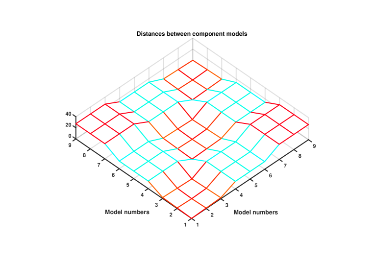
Figure 6: Distances between component models in terms of $\big{\|}G_{u}^{(i)}(s)-G_{u}^{(j)}(s)\big{\|}_{\infty}$

We aim to determine $N$ filters $Q^{(i)}(s)$, $i=1,\ldots,N$, with scalar outputs, having least McMillan degrees and satisfactory dynamics, which fulfill:

• the decoupling conditions: $R_{u}^{(i,i)}(s)=0$, $i=1,\ldots,N$;

• the model detectability condition: $R_{u}^{(i,j)}(s)\neq 0,\quad\forall j\neq i,\;\;i,j=1,\ldots,N$.

Additionally, the resulting model detection performance measures $\|R_{u}^{(i,j)}(s)\|_{\infty}$ should (ideally) reproduce the shape of distances plotted in Fig. 6.

For the design of scalar filters, we used the same $1\times p$ design matrix $H$ for the synthesis of all filters, which has been chosen, after some trials with randomly generated values, as

$$H=[\,0.7645\;\;0.8848\;\;0.5778\;\;0.9026\,]\,.$$

The filter synthesis, performed by employing emdsyn, led to first order stable filters, which, as can be observed in Fig. 7, produces similar shapes of the model detection performance measure as those in Fig. 6.

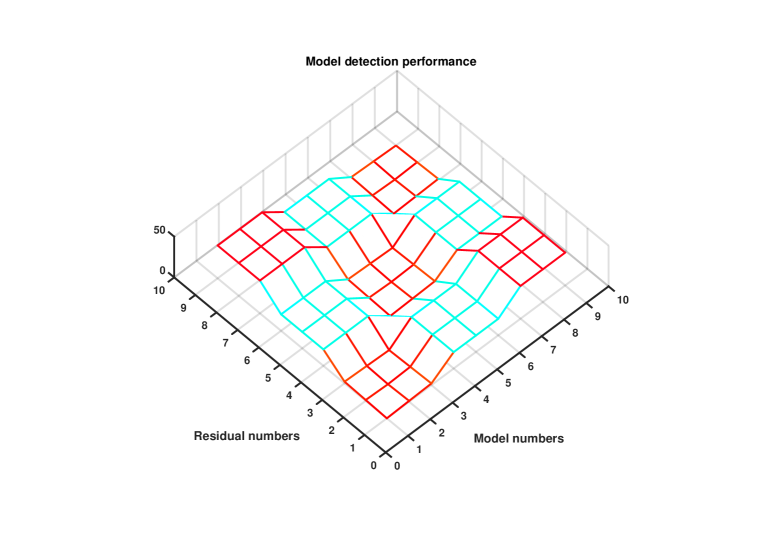
Figure 7: Model detection performance in terms of $\big{\|}R_{u}^{(i,j)}(s)\big{\|}_{\infty}$

In Fig. 8 the step responses from $u_{1}$ (aileron) and $u_{2}$ (rudder) are presented for the $9\times 9$ block array, whose entries are the computed TFMs $R^{(i,j)}(s)$. Each column corresponds to a specific model for which the step responses of the $N$ residuals are computed.

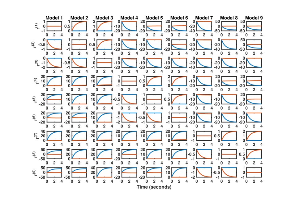
Figure 8: Step responses of $R^{(i,j)}(s)$ from $u_{1}$ (blue) and $u_{2}$ (red) for least order syntheses.

The following script implements the model building, filter synthesis and analysis steps.

% Example - Solution of an exact model detection problem (EMDP)

% Define a lateral aircraft dynamics model (without faults) with
% n  = 4 states
% mu = 2 control inputs
% p  = 4 measurable outputs
A = [-.4492 0.046 .0053 -.9926;
       0    0     1     0.0067;
   -50.8436 0   -5.2184  .722;
    16.4148 0     .0026 -.6627];
Bu = [0.0004 0.0011; 0 0; -1.4161 .2621; -0.0633 -0.1205];
C = eye(4); p = size(C,1); mu = size(Bu,2);

% define the loss of efficiency (LOE) faults as input scaling gains
% Gamma(i,:) = [ 1-rho1(i) 1-rho2(i) ]
Gamma = 1 - [ 0  0 0 .5 .5 .5 1  1 1;
              0 .5 1  0 .5  1 0 .5 1 ]’;
N = size(Gamma,1);  % number of LOE cases

% define a multiple physical fault model Gui = Gu*diag(Gamma(i,:))
sysu = ss(zeros(p,mu,N,1));
for i=1:N
    sysu(:,:,i,1) = ss(A,Bu*diag(Gamma(i,:)),C,0);
end

% setup synthesis model
sysu = mdmodset(sysu,struct(’controls’,1:mu));

% nu-gap distance plots
nugapdist  = mddist(sysu);
figure, mesh(nugapdist), colormap hsv
title(’\nu-gap distances between component models’)
ylabel(’Model numbers’)
xlabel(’Model numbers’)

% H-infinity norm based distance plots
hinfdist  = mddist(sysu,struct(’distance’,’Inf’));
figure, mesh(hinfdist), colormap hsv
title(’H_\infty norm based distances between component models’)
ylabel(’Model numbers’)
xlabel(’Model numbers’)


% call of EMDSYN with the options for stability degree -1 and pole -1 for
% the filters, tolerance and a design matrix H to form a linear combination
% of the left nullspace basis vectors
H = [ 0.7645   0.8848   0.5778   0.9026 ];
emdsyn_options = struct(’sdeg’,-1,’poles’,-1,’HDesign’,H);
[Q,R,info] = emdsyn(sysu,emdsyn_options);

% inspect achieved performance
figure, mesh(info.MDperf), colormap hsv
title(’Distance mapping performance’)
ylabel(’Residual numbers’)
xlabel(’Model numbers’)


% plot the step responses for the internal filter representations
figure
k1 = 0;
for j = 1:N,
  k1 = k1+1;
  k = k1;
  for i=1:N,
    subplot(N,N,k),
    [r,t] = step(R{j,i},4);
    plot(t,r(:,:,1),t,r(:,:,2)),
    if i == 1, title([’Model ’,num2str(j)]), end
    if i == j, ylim([-1 1]), end
    if j == 1, ylabel([’r^(^’, num2str(i),’^)’],’FontWeight’,’bold’), end
    if i == N && j == 5, xlabel(’Time (seconds)’,’FontWeight’,’bold’), end
    k = k+N;
  end
end

4.9.2 amdsyn

Syntax

[Q,R,INFO] = amdsyn(SYSM,OPTIONS)

Description

amdsyn solves the approximate model detection problem (AMDP) (see Section 3.5.2), for a given stable LTI multiple model SYSM containing $N$ models. A bank of $N$ stable and proper residual generation filters $Q^{(i)}(\lambda)$, for $i=1,\ldots,N$, is determined, in the form (37). For each filter $Q^{(i)}(\lambda)$, its associated internal forms $R^{(i,j)}(\lambda)$, for $j=1,\ldots,N$, are determined in accordance with (39).

Input data

SYSM is a multiple model which contains $N$ stable LTI systems in the state-space form

$$\begin{array}[]{rcl}E^{(j)}\lambda x^{(j)}(t)&=&A^{(j)}x^{(j)}(t)+B^{(j)}_{u}u^{(j)}(t)+B^{(j)}_{d}d^{(j)}(t)+B^{(j)}_{w}w^{(j)}(t)\,,\\ y^{(j)}(t)&=&C^{(j)}x^{(j)}(t)+D^{(j)}_{u}u^{(j)}(t)+D^{(j)}_{d}d^{(j)}(t)+D^{(j)}_{w}w^{(j)}(t)\,,\end{array}$$ (206)

where $x^{(j)}(t)\in\mathds{R}^{n^{(j)}}$ is the state vector of the $j$-th system with control input $u^{(j)}(t)\in\mathds{R}^{m_{u}}$, disturbance input $d^{(j)}(t)\in\mathds{R}^{m_{d}^{(j)}}$ and noise input $w^{(j)}(t)\in\mathds{R}^{m_{w}^{(j)}}$, and where any of the inputs components $u^{(j)}(t)$, $d^{(j)}(t)$, or $w^{(j)}(t)$ can be void. The multiple model SYSM is either an array of $N$ LTI systems of the form (206), in which case $m_{d}^{(j)}=m_{d}$ and $m_{w}^{(j)}=m_{w}$ for $j=1,\ldots,N$, or is a $1\times N$ cell array, with SYSM{$j$} containing the $j$-th component system in the form (206). The input groups for $u^{(j)}(t)$, $d^{(j)}(t)$, and $w^{(j)}(t)$ have the standard names ’controls’, ’disturbances’, and ’noise’, respectively.

OPTIONS is a MATLAB structure used to specify various synthesis options and has the following fields:

OPTIONS fields	Description
tol	relative tolerance for rank computations (Default: internally computed)
tolmin	absolute tolerance for observability tests (Default: internally computed)
MDTol	threshold for model detectability checks (Default: $10^{-4}$)
MDGainTol	threshold for strong model detectability checks (Default: $10^{-2}$)
rdim	$N$-dimensional vector or a scalar; for a vector $q$, the $i$-th component $q_{i}$ specifies the desired number of residual outputs for the $i$-th filter Q{$i$}; for a scalar value $\bar{q}$, a vector $q$ with all $N$ components $q_{i}=\bar{q}$ is assumed. (Default:      [ ], in which case: – if OPTIONS.HDesign{$i$} is empty, then $q_{i}=1$, if OPTIONS.minimal = true, or $q_{i}=n_{v}^{(i)}$, the dimension of the left nullspace which underlies the synthesis of Q{$i$}, if OPTIONS.minimal = false and $r_{w}^{(i)}=0$ (see Method); $q_{i}=r_{w}^{(i)}$, if OPTIONS.minimal = false and $r_{w}^{(i)}>0$ (see Method); – if OPTIONS.HDesign{$i$} is nonempty, then $q_{i}$ is the row dimension of the design matrix contained in OPTIONS.HDesign{$i$}.)
emdtest	option to perform extended model detectability tests using both control and disturbance input channels:
	true	–	use both control and disturbance input channels;
	false	–	use only the control channel (default).
smarg	prescribed stability margin for the resulting filters Q{$i$} (Default: -sqrt(eps) for continuous-time component systems;                1-sqrt(eps) for discrete-time component systems.
sdeg	prescribed stability degree for the resulting filters Q{$i$} (Default: $-0.05$ for continuous-time component systems;                 $0.95$ for discrete-time component systems.
poles	complex vector containing a complex conjugate set of desired poles (within the stability margin) to be assigned for the resulting filters Q{$i$} (Default: [ ])
MDFreq	real vector, which contains the frequency values $\omega_{k}$, $k=1,\ldots,n_{f}$, to be used for strong model detectability checks. For each real frequency $\omega_{k}$, there corresponds a complex frequency $\lambda_{k}$ which is used to evaluate the frequency-response gains. Depending on the system type, $\lambda_{k}=\mathrm{i}\omega_{k}$, in the continuous-time case, and $\lambda_{k}=\exp(\mathrm{i}\omega_{k}T)$, in the discrete-time case, where $T$ is the common sampling time of the component systems. (Default: [ ])
nullspace	option to use a specific type of proper nullspace bases:
	true	–	use minimal proper bases;
	false	–	use full-order observer based bases (default) Note: This option can only be used if no disturbance inputs are present in (206) and $\forall j$, $E^{(j)}$ is invertible.
simple	option to compute simple proper bases:
	true	–	compute simple bases; the orders of the basis vectors are provided in INFO.degs;
	false	–	no simple basis computed (default)
minimal	option to perform least order filter syntheses:
	true	–	perform least order syntheses (default);
	false	–	perform full order syntheses.
tcond	maximum allowed value for the condition numbers of the employed
	non-orthogonal transformation matrices (Default: $10^{4}$)
	(only used if OPTIONS.simple = true)
MDSelect	integer vector with increasing elements containing the indices of the desired filters to be designed (Default: $[\,1,\ldots,N\,]$)
HDesign	$N$-dimensional cell array; OPTIONS.HDesign{$i$}, if not empty, is a full row rank design matrix employed for the synthesis of the $i$-th filter. If OPTIONS.HDesign is specified as a full row rank design matrix $H$, then an $N$-dimensional cell array is assumed with OPTIONS.HDesign{$i$} = $H$, for $i=1,\ldots,N$. (Default: [ ]).
epsreg	regularization parameter (Default: 0.1)
sdegzer	prescribed stability degree for zeros shifting (Default: $-0.05$ for a continuous-time system SYSF;                 $0.95$ for a discrete-time system SYSF).
nonstd	option to handle nonstandard optimization problems (see Method):
	1	–	use the quasi-co-outer–co-inner factorization (default);
	2	–	use the modified co-outer–co-inner factorization with the regularization parameter OPTIONS.epsreg;
	3	–	use the Wiener-Hopf type co-outer–co-inner factorization.
	4	–	use the Wiener-Hopf type co-outer-co-inner factorization with zero shifting of the non-minimum phase factor using the stabilization parameter OPTIONS.sdegzer
	5	–	use the Wiener-Hopf type co-outer-co-inner factorization with the regularization of the non-minimum phase factor using the regularization parameter OPTIONS.epsreg

Output data

Q is an $N\times 1$ cell array of filters, where Q{$i$} contains the resulting $i$-th filter in a standard state-space representation

$$\lambda x_{Q}^{(i)}(t) =A_{Q}^{(i)}x_{Q}^{(i)}(t)+B_{Q_{y}}^{(i)}y(t)+B_{Q_{u}}^{(i)}u(t),$$

$$r^{(i)}(t) =C_{Q}^{(i)}x_{Q}^{(i)}(t)+D_{Q_{y}}^{(i)}y(t)+D_{Q_{u}}^{(i)}u(t),$$

where the residual signal $r^{(i)}(t)$ is a $q_{i}$-dimensional vector, with $q_{i}$ specified in OPTIONS.rdim. For each system object Q{$i$}, two input groups ’outputs’ and ’controls’ are defined for $y(t)$ and $u(t)$, respectively, and the output group ’residuals’ is defined for the residual signal $r^{(i)}(t)$. Q{$i$} is empty for all $i$ which do not belong to the index set specified by OPTIONS.MDSelect.

R is an $N\times N$ cell array of filters, where the $(i,j)$-th filter R{$i,j$}, is the internal form of Q{$i$} acting on the $j$-th model. The resulting R{$i,j$} has a standard state-space representation

$$\lambda x_{R}^{(i,j)}(t) =A_{R}^{(i,j)}x_{R}^{(i,j)}(t)+B_{R_{u}}^{(i,j)}u^{(j)}(t)+B_{R_{d}}^{(i,j)}d^{(j)}(t)+B_{R_{w}}^{(i,j)}w^{(j)}(t),$$

$$r^{(i,j)}(t) =C_{R}^{(i,j)}x_{R}^{(i,j)}(t)+D_{R_{u}}^{(i,j)}u^{(j)}(t)+D_{R_{d}}^{(i,j)}d^{(j)}(t)+D_{R_{w}}^{(i,j)}w^{(j)}(t)$$

and the input groups ’controls’, ’disturbances’ and ’noise’ are defined for $u^{(j)}(t)$, $d^{(j)}(t)$, and $w^{(j)}(t)$, respectively, and the output group ’residuals’ is defined for the residual signal $r^{(i,j)}(t)$. R{$i,j$}, $j=1,\ldots,N$ are empty for all $i$ which do not belong to the index set specified by OPTIONS.MDSelect.

INFO is a MATLAB structure containing additional information, as follows:

INFO fields	Description
tcond	$N$-dimensional vector; INFO.tcond$(i)$ contains the maximum of the condition numbers of the non-orthogonal transformation matrices used to determine the $i$-th filter Q{$i$}; a warning is issued if any INFO.tcond$(i)$ $\geq$ OPTIONS.tcond.
degs	$N$-dimensional cell array; if OPTIONS.simple = true, then a nonempty INFO.degs{$i$} contains the orders of the basis vectors of the employed simple nullspace basis for the synthesis of the $i$-th filter component Q{$i$}; if OPTIONS.simple = false, then a nonempty INFO.degs{$i$} contains the degrees of the basis vectors of an equivalent polynomial nullspace basis; INFO.degs{$i$} = [ ] for all $i$ which do not belong to the index set specified by OPTIONS.MDSelect.
MDperf	$N\times N$-dimensional array containing the achieved model detection performance measure, given as the gains associated with the internal representations (see Method). $\texttt{INFO.MDperf($i,j$)}=-1$, for $j=1,\ldots,N$ and for all $i$ which do not belong to the index set specified by OPTIONS.MDSelect.
HDesign	$N$-dimensional cell array, where INFO.HDesign{$i$} contains the $i$-th design matrix $H^{(i)}$ employed for the synthesis of the $i$-th filter (see Method)
MDgap	$N$-dimensional vector, which contains the achieved noise gaps. INFO.MDgap$(i)$ contains the $i$-th gap $\eta_{i}$ achieved by the $i$-th filter (see Method).

Method

An extension of the Procedure AMD from [16, Sect. 6.3] is implemented, which relies on the nullspace-based synthesis method proposed in [10]. Assume that the $j$-th model has the input-output form

$${\mathbf{y}}^{(j)}(\lambda)=G_{u}^{(j)}(\lambda){\mathbf{u}}^{(j)}(\lambda)+G_{d}^{(j)}(\lambda){\mathbf{d}}^{(j)}(\lambda)+G_{w}^{(j)}(\lambda){\mathbf{w}}^{(j)}(\lambda)$$ (207)

and the resulting $i$-th filter $Q^{(i)}(\lambda)$ has the input-output form

$${\mathbf{r}}^{(i)}(\lambda)=Q^{(i)}(\lambda)\left[\begin{array}[]{c}{\mathbf{y}}(\lambda)\\ {\mathbf{u}}(\lambda)\end{array}\right]\,.$$ (208)

The synthesis method, which underlies Procedure AMD, essentially determines each filter $Q^{(i)}(\lambda)$ as a stable rational left annihilator of

$$G^{(i)}(\lambda):=\left[\begin{array}[]{cc}G_{u}^{(i)}(\lambda)&G_{d}^{(i)}(\lambda)\\ I_{m_{u}}&0\end{array}\right],$$

such that for $i\neq j$ we have $[\,R_{u}^{(i,j)}(\lambda)\;R_{d}^{(i,j)}(\lambda)\,]\neq 0$, where

$$R^{(i,j)}(\lambda):=[\,R_{u}^{(i,j)}(\lambda)\;R_{d}^{(i,j)}(\lambda)\;R_{w}^{(i,j)}(\lambda)\,]=Q^{(i)}(\lambda)\left[\begin{array}[]{ccc}G_{u}^{(j)}(\lambda)&G_{d}^{(j)}(\lambda)&G_{w}^{(j)}(\lambda)\\ I_{m_{u}}&0&0\end{array}\right]$$

is the internal form of $Q^{(i)}(\lambda)$ with respect to the $j$-th model. Additionally, the gap $\eta_{i}$ achieved by the $i$-th filter is maximized.

The resulting $N\times N$ matrix INFO.MDperf can be used for the assessment of the achieved distance mapping performance of the resulting model detection filters (see Section 3.6.3 for definitions). If OPTIONS.MDFreq is empty, then INFO.MDperf$(i,j)=\big{\|}\big{[}\,R_{u}^{(i,j)}(\lambda)\;R_{d}^{(i,j)}(\lambda)\,\big{]}\big{\|}_{\infty}$ if OPTIONS.emdtest = true and INFO.MDperf$(i,j)=\big{\|}R_{u}^{(i,j)}(\lambda)\big{\|}_{\infty}$ if OPTIONS.emdtest = false, and, ideally, represents a measure of the distance between the $i$-th and $j$-th component systems. If OPTIONS.MDFreq contains a set of $n_{f}$ real frequency values $\omega_{k}$, $k=1,\ldots,n_{f}$ and $\lambda_{k}$, $k=1,\ldots,n_{f}$ are the corresponding complex frequencies (see the description of OPTIONS.MDFreq), then INFO.MDperf$(i,j)$ $=\max_{k}\big{\|}\big{[}\,R_{u}^{(i,j)}(\lambda_{k})\;R_{d}^{(i,j)}(\lambda_{k})\,\big{]}\big{\|}_{\infty}$ if OPTIONS.emdtest = true and INFO.MDperf$(i,j)=$ $\max_{k}\big{\|}R_{u}^{(i,j)}(\lambda_{k})\big{\|}_{\infty}$ if OPTIONS.emdtest = false. In this case, the entry INFO.MDperf$(i,j)$ ideally represents a measure of the maximum distance between the frequency responses of the $i$-th and $j$-th component systems, evaluated in the selected set of frequency values. If OPTIONS.normalize = true, then for each row $i$, the filters Q{i} and R{i,j} are scaled such that the least value of INFO.MDperf$(i,j)$ for $i\neq j$ is normalized to one. The standard normalization is performed if OPTIONS.normalize = false, in which case INFO.MDperf$(1,j)$ = INFO.MDperf$(j,1)$ for $j>1$.

The $N$-dimensional vector INFO.MDgap, contains the resulting noise gaps $\eta_{i}$, for $i=1,\ldots,N$ (see Section 3.6.5 for definitions). If OPTIONS.MDFreq is empty, then $\eta_{i}$ is evaluated as

$$\eta_{i}:=\min_{j\neq i}\big{\|}\big{[}\,R_{u}^{(i,j)}(\lambda)\;R_{d}^{(i,j)}(\lambda)\,\big{]}\big{\|}_{\infty}/\big{\|}R_{w}^{(i,i)}(\lambda)\big{\|}_{\infty},$$ (209)

if OPTIONS.emdtest = true and

$$\eta_{i}:=\min_{j\neq i}\big{\|}R_{u}^{(i,j)}(\lambda)\big{\|}_{\infty}/\big{\|}R_{w}^{(i,i)}(\lambda)\big{\|}_{\infty},$$ (210)

if OPTIONS.emdtest = false. If OPTIONS.MDFreq contains a set of $n_{f}$ real frequency values $\omega_{k}$, $k=1,\ldots,n_{f}$ and $\lambda_{k}$, $k=1,\ldots,n_{f}$ are the corresponding complex frequencies (see the description of OPTIONS.MDFreq), then

$$\eta_{i}:=\min_{j\neq i}\max_{k}\big{\|}\big{[}\,R_{u}^{(i,j)}(\lambda_{k})\;R_{d}^{(i,j)}(\lambda_{k})\,\big{]}\big{\|}_{2}/\big{\|}R_{w}^{(i,i)}(\lambda)\big{\|}_{\infty},$$ (211)

if OPTIONS.emdtest = true and

$$\eta_{i}:=\min_{j\neq i}\max_{k}\big{\|}R_{u}^{(i,j)}(\lambda_{k})\big{\|}_{2}/\big{\|}R_{w}^{(i,i)}(\lambda)\big{\|}_{\infty},$$ (212)

if OPTIONS.emdtest = false.

Each filter $Q^{(i)}(\lambda)$ is determined in the product form

$$Q^{(i)}(\lambda)=Q_{4}^{(i)}(\lambda)Q_{3}^{(i)}(\lambda)Q_{2}^{(i)}(\lambda)Q_{1}^{(i)}(\lambda),$$ (213)

where the factors are determined as follows:

• $Q_{1}^{(i)}(\lambda)=N_{l}^{(i)}(\lambda)$, with $N_{l}^{(i)}(\lambda)$ a $\big{(}p-r_{d}^{(i)}\big{)}\times(p+m_{u})$ proper rational left nullspace basis satisfying $N_{l}^{(i)}(\lambda)G^{(i)}(\lambda)=0$, with $r_{d}^{(i)}:=\text{rank}\,G_{d}^{(i)}(\lambda)$; ($n_{v}^{(i)}:=p-r_{d}^{(i)}$ is the number of basis vectors)

• $Q_{2}^{(i)}(\lambda)$ is an admissible regularization factor guaranteeing model detectability;

• $Q_{3}^{(i)}(\lambda)$ represents an optimal choice to maximize the $i$-th gap $\eta_{i}$ in (209) – (212);

• $Q_{4}^{(i)}(\lambda)$ is a stable invertible factor determined such that $Q^{(i)}(\lambda)$ has a desired dynamics.

The computations of individual factors depend on the user’s options and the optimization problem features. Specific choices are discussed in what follows.

Computation of $Q_{1}^{(i)}(\lambda)$

If OPTIONS.nullspace = true, then the left nullspace basis $N_{l}^{(i)}(\lambda)$ is determined as a stable minimal proper rational basis, or, if OPTIONS.nullspace = false (the default option) and $m_{d}^{(i)}=0$, then the simple observer based basis $N_{l}^{(i)}(\lambda)=[\,I\;-G_{u}^{(i)}(\lambda)\,]$ is employed. If $N_{l}^{(i)}(\lambda)$ is a minimal rational basis and if OPTIONS.simple = true, then $N_{l}^{(i)}(\lambda)$ is determined as a simple rational basis and the orders of the basis vectors are provided in INFO.degs. These are also the degrees of the basis vectors of an equivalent polynomial nullspace basis. The dynamics of $Q_{1}^{(i)}(\lambda)$ is specified via OPTIONS.sdeg and OPTIONS.poles.

Computation of $Q_{2}^{(i)}(\lambda)$

Let $r_{w}^{(i)}$ be the rank of $\overline{G}_{w}^{(i,i)}(\lambda):=Q_{1}^{(i)}(\lambda)\left[\begin{smallmatrix}G_{w}^{(i)}(\lambda)\\ 0\end{smallmatrix}\right]$ and let $q_{i}$ be the desired number of residual outputs for the $i$-th filter. If OPTIONS.rdim is nonempty, then $q_{i}=\texttt{OPTIONS.rdim}\{i\}$, while if OPTIONS.rdim is empty a default value of $q_{i}$ is defined depending on the setting of $\texttt{OPTIONS.HDesign}\{i\}$ and OPTIONS.minimal. If $\texttt{OPTIONS.HDesign}\{i\}$ is nonempty, then $q_{i}$ is the row dimension of the design matrix contained in $\texttt{OPTIONS.HDesign}\{i\}$. If $\texttt{OPTIONS.HDesign}\{i\}$ is empty, then $q_{i}=1$ if OPTIONS.minimal = true. If OPTIONS.minimal = false and $r_{w}^{(i)}=0$, then $q_{i}=p-r_{d}^{(i)}$, while if $r_{w}^{(i)}>0$, then $q_{i}=r_{w}^{(i)}$.

If OPTIONS.minimal = false, then $Q_{2}^{(i)}(\lambda)=M^{(i)}(\lambda)H^{(i)}$, where $H^{(i)}$ is a suitable $q_{i}\times\big{(}p-r_{d}^{(i)}\big{)}$ full row rank design matrix and $M^{(i)}(\lambda)$ is a stable invertible transfer function matrix determined such that $Q_{2}^{(i)}(\lambda)Q_{1}^{(i)}(\lambda)$ has a desired dynamics (specified via OPTIONS.sdeg and OPTIONS.poles). $H^{(i)}$ is set as follows. If OPTIONS.HDesign$\{i\}$ is nonempty, then $H^{(i)}=\texttt{OPTIONS.HDesign}\{i\}$. If OPTIONS.HDesign$\{i\}$ is empty, the matrix $H^{(i)}$ is chosen to build $q_{i}$ linear combinations of the $p-r_{d}^{(i)}$ left nullspace basis vectors, such that $H^{(i)}Q_{1}^{(i)}(\lambda)$ has full row rank. If $q_{i}=p-r_{d}^{(i)}$ then the choice $H^{(i)}=I_{p-r_{d}^{(i)}}$ is used, otherwise $H^{(i)}$ is chosen a randomly generated $q_{i}\times\big{(}p-r_{d}^{(i)}\big{)}$ real matrix.

If OPTIONS.minimal = true, then $Q_{2}^{(i)}(\lambda)$ is a $q_{i}\times\big{(}p-r_{d}^{(i)}\big{)}$ transfer function matrix, with $q_{i}$ chosen as above. $Q_{2}^{(i)}(\lambda)$ is determined in the form

$$Q_{2}^{(i)}(\lambda)=M^{(i)}(\lambda)\widetilde{Q}_{2}^{(i)}(\lambda)\,,$$

where $\widetilde{Q}_{2}^{(i)}(\lambda):=H^{(i)}+Y_{2}^{(i)}(\lambda)$, $\widetilde{Q}_{2}^{(i)}(\lambda)Q_{1}^{(i)}(\lambda)$ $\big{(}\!=H^{(i)}N_{l}^{(i)}(\lambda)+Y_{2}^{(i)}(\lambda)N_{l}^{(i)}(\lambda)\big{)}$ and $Y_{2}^{(i)}(\lambda)$ are the least order solution of a left minimal cover problem [15], and $M^{(i)}(\lambda)$, a stable invertible transfer function matrix determined such that $M^{(i)}(\lambda)\widetilde{Q}_{2}^{(i)}(\lambda)Q_{1}^{(i)}(\lambda)$ has a desired dynamics. If OPTIONS.HDesign$\{i\}$ is nonempty, then $H^{(i)}=\texttt{OPTIONS.HDesign}\{i\}$, and if OPTIONS.HDesign$\{i\}$ is empty, then a suitable randomly generated $H^{(i)}$ is employed (see above).

Note: The stabilization with $M^{(i)}(\lambda)$ is only performed if $r_{w}^{(i)}=0$ (i.e., to also cover the case of an exact synthesis).

The structure field INFO.HDesign$\{i\}$ contains the employed value of the design matrix $H^{(i)}$.

Computation of $Q_{3}^{(i)}(\lambda)$

Let define $\widetilde{G}_{w}^{(i,i)}(\lambda):=Q_{2}^{(i)}(\lambda)\overline{G}_{w}^{(i,i)}(\lambda)$ and let $\tilde{r}_{w}^{(i)}=\mathop{\mathrm{rank}}\widetilde{G}_{w}^{(i,i)}(\lambda)$, which satisfies $\tilde{r}_{w}^{(i)}\leq q_{i}$. If $\tilde{r}_{w}^{(i)}=0$ then $Q_{3}^{(i)}(\lambda)=I$. If $\tilde{r}_{w}^{(i)}>0$, then the quasi-co-outer–co-inner factorization of $\widetilde{G}_{w}^{(i,i)}(\lambda)$ is computed as

$$\widetilde{G}_{w}^{(i,i)}(\lambda)=R_{wo}^{(i)}(\lambda)R_{wi}^{(i)}(\lambda),$$

where $R_{wo}^{(i)}(\lambda)$ is a (full column rank) quasi-co-outer factor and $R_{wi}^{(i)}(\lambda)$ is a (full row rank) co-inner factor. In the standard case $R_{wo}^{(i)}(\lambda)$ is outer (i.e., has no zeros on the boundary of the stability domain $\partial\mathds{C}_{s}$) and thus, there exists a stable left inverse $\big{(}R_{wo}^{(i)}(\lambda)\big{)}^{-L}$ such that $\big{(}R_{wo}^{(i)}(\lambda)\big{)}^{-L}R_{wo}^{(i)}(\lambda)=I$. In this case, we choose $Q_{3}^{(i)}(\lambda)=\big{(}R_{wo}^{(i)}(\lambda)\big{)}^{-L}$. This is an optimal choice which ensures that the maximal gap $\eta_{i}$ is achieved by the $i$-th filter (see below). If $\tilde{r}_{w}=q_{i}$ (the usual case), then $Q_{3}^{(i)}(\lambda)$ is simply $Q_{3}^{(i)}(\lambda)=\big{(}R_{wo}^{(i)}(\lambda)\big{)}^{-1}$.

In the non-standard case $R_{wo}^{(i)}(\lambda)$ is only quasi-outer and thus, has zeros on the boundary of the stability domain $\partial\mathds{C}_{s}$. Depending on the selected option to handle nonstandard optimization problems OPTIONS.nonstd, several choices are possible for $Q_{3}^{(i)}(\lambda)$ in this case:

• If OPTIONS.nonstd = 1, then $Q_{3}^{(i)}(\lambda)=\big{(}R_{wo}^{(i)}(\lambda)\big{)}^{-L}$ is used, where all spurious poles of the left inverse are assigned to values specified via OPTIONS.sdeg and OPTIONS.poles.

• If OPTIONS.nonstd = 2, then a modified co-outer–co-inner factorization of $[\,R_{wo}^{(i)}(\lambda)\;\epsilon I\,]$ is computed, whose co-outer factor $R_{wo,\epsilon}^{(i)}(\lambda)$ satisfies

  $$R_{wo,\epsilon}^{(i)}(\lambda)\big{(}R_{wo,\epsilon}^{(i)}(\lambda)\big{)}^{\sim}=\epsilon^{2}I+R_{wo}^{(i)}(\lambda)\big{(}R_{wo}^{(i)}(\lambda)\big{)}^{\sim}.$$

  Then $Q_{3}^{(i)}(\lambda)=\big{(}R_{wo,\epsilon}^{(i)}(\lambda)\big{)}^{-L}$ is used. The value of the regularization parameter $\epsilon$ is specified via OPTIONS.epsreg.

• If OPTIONS.nonstd = 3, then a Wiener-Hopf type co-outer–co-inner factorization is computed in the form

  $$\widetilde{G}_{w}^{(i,i)}(\lambda)=R_{wo}^{(i)}(\lambda)R_{wb}^{(i)}(\lambda)R_{wi}^{(i)}(\lambda),$$ (214)

  where $R_{wo}^{(i)}(\lambda)$ is co-outer, $R_{wi}^{(i)}(\lambda)$ is co-inner, and $R_{wb}^{(i)}(\lambda)$ is a square stable factor whose zeros are precisely the zeros of $\widetilde{G}_{w}^{(i,i)}(\lambda)$ in $\partial\mathds{C}_{s}$. $Q_{3}^{(i)}(\lambda)$ is determined as before $Q_{3}^{(i)}(\lambda)=\big{(}R_{wo}^{(i)}(\lambda)\big{)}^{-L}$.

• If OPTIONS.nonstd = 4, then the Wiener-Hopf type co-outer–co-inner factorization (214) is computed and $Q_{3}^{(i)}(\lambda)$ is determined as $Q_{3}^{(i)}(\lambda)=\big{(}R_{wb}^{(i)}(\tilde{\lambda})\big{)}^{-1}\big{(}R_{wo}^{(i)}(\lambda)\big{)}^{-1}$, where $\tilde{\lambda}$ is a small perturbation of $\lambda$ to move all zeros of $R_{wb}^{(i)}(\lambda)$ into the stable domain. In the continuous-time case $\tilde{s}=\frac{s-\beta_{z}}{1-\beta_{z}s}$, while in the discrete-time case $\tilde{z}=z/\beta_{z}$, where the zero shifting parameter $\beta_{z}$ is the prescribed stability degree for the zeros specified in OPTIONS.sdegzer. For the evaluation of $R_{wb}^{(i)}(\tilde{\lambda})$, a suitable bilinear transformation is performed.

• If OPTIONS.nonstd = 5, then the Wiener-Hopf type co-outer–co-inner factorization (214) is computed and $Q_{3}^{(i)}(\lambda)$ is determined as $Q_{3}^{(i)}(\lambda)=\big{(}R_{wb,\epsilon}^{(i)}(\lambda)\big{)}^{-1}\big{(}R_{wo}^{(i)}(\lambda)\big{)}^{-1}$, where $R_{wb,\epsilon}^{(i)}(\lambda)$ is the co-outer factor of the co-outer–co-inner factorization of $\big{[}\,R_{wb}^{(i)}(\lambda)\;\epsilon I\,\big{]}$ and satisfies

  $$R_{wb,\epsilon}^{(i)}(\lambda)\big{(}R_{wb,\epsilon}^{(i)}(\lambda)\big{)}^{\sim}=\epsilon^{2}I+R_{wb}^{(i)}(\lambda)\big{(}R_{wb}^{(i)}(\lambda)\big{)}^{\sim}.$$

  The value of the regularization parameter $\epsilon$ is specified via OPTIONS.epsreg.

A typical feature of the non-standard case is that, with the exception of using the option OPTIONS.nonstd = 3, all other choices of OPTIONS.nonstd lead to a poor dynamical performance of the resulting filter, albeit arbitrary large noise gaps $\eta_{i}$ can be occasionally achieved.

Computation of $Q_{4}^{(i)}(\lambda)$

In the standard case, $Q_{4}^{(i)}(\lambda)=I$. In the non-standard case, $Q_{4}^{(i)}(\lambda)$ is a stable invertible transfer function matrix determined such that $Q^{(i)}(\lambda)$ in (213) has a desired dynamics (specified via OPTIONS.sdeg and OPTIONS.poles).

Example

Example 16.

This is Example 6.2 from the book [16], which deals with a continuous-time state-space model, describing, in the fault-free case, the lateral dynamics of an F-16 aircraft with the matrices

$${A^{(1)}\!=\!\left[\begin{array}[]{rrrr}-0.4492&0.046&0.0053&-0.9926\\ 0&0&1.0000&0.0067\\ -50.8436&0&-5.2184&0.7220\\ 16.4148&0&0.0026&-0.6627\end{array}\right],\;\;B_{u}^{(1)}\!=\!\left[\begin{array}[]{rr}0.0004&0.0011\\ 0&0\\ -1.4161&0.2621\\ -0.0633&-0.1205\end{array}\right],}\;\,B_{w}^{(1)}\!=\![\,I_{4}\;0_{4\times 2}\,]\;,$$

$$C^{(1)}=\left[\begin{array}[]{cccc}57.2958&0&0&0\\ 0&57.2958&0&0\end{array}\right],\;\,D_{u}^{(1)}=0_{2\times 2},\;\,D_{w}^{(1)}=[\,0_{2\times 4}\;\;I_{2}\,]\,.$$

The four state variables are the sideslip angle, roll angle, roll rate and yaw rate, and the two input variables are the aileron deflection and rudder deflection. The two measured outputs are the sideslip angle and roll angle, and, additionally input noise and output noise are included in the model. The component system matrices in (206) are defined for $i=1,2,\ldots,N$ as: $E^{(i)}=I_{4}$, $A^{(i)}=A^{(1)}$, $C^{(i)}=C^{(1)}$, $B_{w}^{(i)}=B^{(1)}_{w}$, $D_{w}^{(i)}=D^{(1)}_{w}$, and $B_{u}^{(i)}=B^{(1)}_{u}\Gamma^{(i)}$, where $\Gamma^{(i)}=\mathop{\mathrm{diag}}\big{(}1-\rho_{1}^{(i)},1-\rho_{2}^{(i)}\big{)}$ and $\big{(}\rho_{1}^{(i)},\rho_{2}^{(i)}\big{)}$ are the values of parameters $(\rho_{1},\rho_{2})$ on the chosen grid points:

$\rho_{1}:$	0	0	0	0.5	0.5	0.5	1	1	1
$\rho_{2}:$	0	0.5	1	0	0.5	1	0	0.5	1

.

The TFMs $G_{u}^{(i)}(s)$ and $G_{w}^{(i)}(s)$ of the $i$-th system can be expressed as

$$G_{u}^{(i)}(s)=G_{u}^{(1)}(s)\Gamma^{(i)},\quad G_{w}^{(i)}(s)=G_{w}^{(1)}(s)\;,$$ (215)

where

$$G_{u}^{(1)}(s)=C^{(1)}\big{(}sI-A^{(1)}\big{)}^{-1}B^{(1)}_{u},\quad G_{w}^{(1)}(s)=C^{(1)}\big{(}sI-A^{(1)}\big{)}^{-1}B^{(1)}_{w}+D^{(1)}_{w}\,.$$

The individual fault models correspond to different degrees of surface efficiency degradation. The values $\big{(}\rho_{1}^{(1)},\rho_{2}^{(1)}\big{)}=(0,0)$ correspond to the fault-free situation, while $G_{u}^{(N)}(s)=0$ describes the case of complete failure.

The approximate model detection problem addresses the synthesis of model detection filters for the detection and identification of loss of efficiency of the two flight actuators, which control the deflections of the aileron and rudder, in the presence of noise inputs. For the design of the model detection system, we aim to determine the $N$ filters $Q^{(i)}(s)$, $i=1,\ldots,N$ having satisfactory dynamic responses and exhibiting the maximally achievable gaps.

In Fig. 9 the time responses of the residual evaluation signals $\theta_{i}(t)$ are presented, where $\theta_{i}(t)$ are computed using a Narendra-type evaluation filter [3] with input $\|r^{(i)}(t)\|_{2}^{2}$ and parameters $\alpha=0.9$, $\beta=0.1$, $\gamma=10$ (see also Remark 3.13 in [16]). The control inputs have been chosen as follows: $u_{1}(t)$ is a step of amplitude 0.3 added to a square wave of period $2\pi$, and $u_{2}(t)$ is a step of amplitude 1.5 added to a sinus function of unity amplitude and period $\pi$. The noise inputs are zero mean white noise of amplitude 0.01 for the input noise and 0.03 for the measurement noise. Each column corresponds to a specific model for which the time responses of the $N$ residual evaluation signals are computed. The achieved typical structure matrix for model detection (with zeros down the diagonal) can easily be read out from this signal based assessment, even in presence of noise.

Figure 9: Time responses of evaluation signals for optimal syntheses

The following script implements the model building, synthesis and analysis steps.

% Example - Solution of an approximate model detection problem (AMDP)

% Define a lateral aircraft dynamics model (without faults) with
% n  = 4 states
% mu = 2 control inputs
% p  = 2 measurable outputs
% mw = 6 noise inputs

A = [-.4492 .046  .0053 -.9926;
       0    0     1      .0067;
   -50.8436 0   -5.2184  .722;
    16.4148 0     .0026 -.6627];
Bu = [.0004 .0011; 0 0; -1.4161 .2621; -.0633 -.1205];
[n,mu] = size(Bu); p = 2; mw = n+p; m = mu+mw;
Bw = eye(n,mw);
C = 180/pi*eye(p,n);  Du = zeros(p,mu); Dw = [zeros(p,n) eye(p)];

% define the loss of efficiency (LOE) faults as input scaling gains
% Gamma(i,:) = [ 1-rho1(i) 1-rho2(i) ]
Gamma = 1 - [ 0  0 0 .5 .5 .5 1  1 1;
              0 .5 1  0 .5  1 0 .5 1 ]’;
N = size(Gamma,1);  % number of LOE cases

% define a multiple physical fault model Gui = Gu*diag(Gamma(i,:))
sysuw = ss(zeros(p,mu+mw,N,1));
for j = 1:N
    sysuw(:,:,j,1) = ss(A,[Bu*diag(Gamma(j,:)) Bw],C,[Du Dw]);
end

% setup synthesis model
sysuw = mdmodset(sysuw,struct(’controls’,1:mu,’noise’,mu+(1:mw)));

% use nonminimal design with  AMDSYN with stability degree -1 and poles  at -1
opt_amdsyn = struct(’sdeg’,-1,’poles’,-1,’minimal’,false);
[Q,R,info] = amdsyn(sysuw,opt_amdsyn);
info.MDperf, info.MDgap

% inspect achieved performance
figure, mesh(info.MDperf), colormap hsv
title(’Model detection performance’)
ylabel(’Residual numbers’)
xlabel(’Model numbers’)

% generate input signals for Ex. 6.2
d = diag([ 1 1 0.01 0.01 0.01 0.01 0.03 0.03]);
t = (0:0.01:10)’;  ns = length(t);
usin = gensig(’sin’,pi,t(end),0.01)+1.5;
usquare = gensig(’square’,pi*2,t(end),0.01)+0.3;
u = [ usquare usin (rand(ns,mw)-0.5)]*d;

% plot the step responses for the internal filter representations
figure
k1 = 0; alpha = 0.9; beta = 0.1; gamma = 10;
for j = 1:N,
  k1 = k1+1; k = k1;
  for i=1:N,
    subplot(N,N,k),
    [r,t] = lsim(R{j,i},u,t);
    % use a Narendra filter with (alpha,beta,gamma) = (0.9,0.1,10)
    theta = alpha*sqrt(r(:,1).^2+r(:,2).^2)+...
        beta*sqrt(lsim(tf(1,[1 gamma]),r(:,1).^2+r(:,2).^2,t));
    plot(t,theta),
    if i == 1, title([’Model ’,num2str(j)]), end
    if i == j, ylim([0 1]), end
    if j == 1, ylabel([’\theta_’, num2str(i)],’FontWeight’,’bold’), end
    if i == N && j == 5, xlabel(’Time (seconds)’,’FontWeight’,’bold’), end
    k = k+N;
  end
end

Refs.1Refs.1ReferencesReferencesRefs.1

Appendix A Installing FDITOOLS

FDITOOLS runs with MATLAB R2015b (or later versions) under 64-bit Windows 7 (or later). Additionally, the Control System Toolbox (Version 9.10 or later) and the Descriptor Systems Tools (DSTOOLS) collection (Version 0.64 or later) are necessary to be installed. To install FDITOOLS, perform the following steps:

• download FDITOOLS and DSTOOLS as zip files from Bitbucket

• create on your computer the directories fditools and dstools

• extract, using any unzip utility, the functions of the FDITOOLS and DSTOOLS collections in the corresponding directories fditools and dstools, respectively

• start MATLAB and put the directories fditools and dstools on the MATLAB path, by using the pathtool command; for repeated use, save the new MATLAB search path, or alternatively, use the addpath command to set new path entries in startup.m

• try out the installation by running the demonstration script FDIToolsdemo.m

Note: The software accompanying the book [16] can be also downloaded as a zip file, which also includes FDITOOLS V0.2 and DSTOOLS V0.5. To install and execute the example and case-study scripts listed in the book, follow the steps indicated in the web page. An updated collection of MATLAB scripts with examples is also available from Bitbucket.

Appendix B Current Contents.m File

The M-functions available in the current version of FDITOOLS are listed in the current version of the Contents.m file, given below:

% FDITOOLS - Fault detection and isolation filter synthesis tools.
% Version 1.0           30-November-2018
% Copyright 2016-2018 A. Varga
%
% Demonstration.
%   FDIToolsdemo - Demonstration of FDITOOLS.
%
% Setup of synthesis models.
%   fdimodset  - Setup of models for solving FDI synthesis problems.
%   mdmodset   - Setup of models for solving model detection synthesis problems.
%
% Analysis.
%   fdigenspec - Generation of achievable FDI specifications.
%   fdichkspec - Checking the feasability of a set of specifications.
%   mddist     - Computation of distances between component models.
%   mddist2c   - Computation of distances to a set of component models.
%
% Performance evaluation of FDI filters
%   fditspec   - Computation of the weak or strong structure matrix.
%   fdisspec   - Computation of the strong structure matrix.
%   fdifscond  - Fault sensitivity condition of FDI filters.
%   fdif2ngap  - Fault-to-noise gap of FDI filters.
%   fdimmperf  - Model-matching performance of FDI filters.
%
% Performance evaluation of model detection filters
%   mdperf     - Distance mapping performance of model detection filters.
%   mdmatch    - Distance matching performance of model detection filters.
%   mdgap      - Noise gaps of model detection filters.
%
% Synthesis of FDI filters.
%   efdsyn     - Exact synthesis of fault detection filters.
%   afdsyn     - Approximate synthesis of fault detection filters.
%   efdisyn    - Exact synthesis of fault detection and isolation filters.
%   afdisyn    - Approximate synthesis of fault detection and isolation filters.
%   emmsyn     - Exact model matching based synthesis of FDI filters.
%   ammsyn     - Approximate model matching based synthesis of FDI filters.
%
% Synthesis of model detection filters.
%   emdsyn     - Exact synthesis of model detection filters.
%   amdsyn     - Approximate synthesis of model detection filters.
%
% Miscellaneous.
%   hinfminus  - H-(infinity-) index of a stable transfer function matrix.
%   hinfmax    - Maximum of H-inf norms of columns of a transfer function matrix.
%   efdbasesel - Selection of admissible basis vectors to solve the EFDP.
%   afdbasesel - Selection of admissible basis vectors to solve the AFDP.
%   emmbasesel - Selection of admissible basis vectors to solve the strong EFDIP.
%   ammbasesel - Selection of admissible basis vectors to solve the strong AFDIP.
%   emdbasesel - Selection of admissible basis vectors to solve the EMDP.
 

Appendix C FDITOOLS Release Notes

The FDITOOLS Release Notes describe the changes introduced in the successive versions of the FDITOOLS collection, as new features, enhancements to functions, or major bug fixes. The following versions of FDITOOLS have been released:

Version	Release date	Comments
V0.2	December 31, 2016	Initial version accompanying the book [16].
V0.21	February 15, 2017	Enhanced user interface of function genspec.
V0.3	April 7, 2017	New function for the exact model-matching based synthesis.
V0.4	August 31, 2017	New function for the exact synthesis of model detection filters and substantial enhancements of most functions. The option to use “design matrices” has been added to all synthesis functions.
V0.8	February 28, 2018	Complete set of functions for the approximate synthesis of fault detection and model detection filters implemented.
V0.85	July 7, 2018	New functions for performance evaluation of fault detection filters have been implemented together with notable enhancements of existing analysis functions. New synthesis options have been implemented in almost all synthesis functions (e.g., using an observer-based nullspace basis, option to perform exact synthesis for approximate synthesis functions, etc.)
V0.87	August 15, 2018	Enhancements of the approximate model-matching synthesis function performed and a new function implemented for model-matching performance evaluation.
V1.0	November 30, 2018	Many enhancements of the approximate synthesis functions performed, by using the version V0.71 of DSTOOLS. A set of new functions have been implemented for the analysis of multiple models and performance evaluation of model detection filters.

C.1 Release Notes V0.2

This is the initial version of the FDITOOLS collection of M-functions, which accompanies the book [16]. All numerical results presented in this book have been obtained using this version of FDITOOLS.

C.1.1 New Features

The M-functions available in the Version 0.2 of FDITOOLS are listed below:

% FDITools - Fault detection and isolation filter synthesis tools.
% Version 0.2            31-Dec-2016
% Copyright 2017 A. Varga
%
% Demonstration.
%   FDIToolsdemo - Demonstration of FDITools.
%
% Analysis functions.
%   fditspec   - Computation of the structure matrix of a system.
%   fdisspec   - Computation of the strong structure matrix of a system.
%   genspec    - Generation of achievable fault detection specifications.
%
% Synthesis functions.
%   efdsyn     - Exact synthesis of fault detection filters.
%   efdisyn    - Exact synthesis of fault detection and isolation filters.
%
% Miscellaneous.
%   efdbasesel - Selection of admissible basis vectors to solve the EFDP.
%

C.2 Release Notes V0.21

Version 0.21, dated February 15, 2017, is a minor improvement over version 0.2 of FDITOOLS.

C.2.1 New Features

A new version of the function genspec is provided, with an enhanced user interface. The new calling syntax, which also covers the previously used calling syntax, is similar to that used by the synthesis functions and allows the direct handling of systems having control, disturbance and additive fault inputs.

C.3 Release Notes V0.3

Version 0.3, dated April 7, 2017, provides a complete set of functions implementing the exact synthesis approaches of fault detection and isolation filters.

C.3.1 New Features

Two new functions have been implemented:

• The function emmsyn is provided for the exact synthesis of fault detection and isolation filters, by using an exact model-matching approach.

• The function emmbasesel is provided for the selection of admissible left nullspace basis vectors to solve the strong exact fault detection and isolation problem, using an exact model-matching approach.

C.4 Release Notes V0.4

Version 0.4, dated August 31, 2017, is a major new release, including substantial revisions of most functions, by adding exhaustive input parameter checks, new user options and several enhancements and simplifications of the implemented codes. Besides these modifications, two new functions have been implemented for the exact synthesis of model detection filters.

C.4.1 New Features

Two new functions have been implemented:

• The function emdsyn is provided for the exact synthesis of model detection filters, by using a nullspace-based synthesis approach.

• The function emdbasesel is provided for the selection of admissible left nullspace basis vectors for solving the exact model detection problem.

Several new features have been implemented:

• The functionality of fditspec has been enhanced, by generating a three-dimensional structure matrix in the case of several frequency values specified at input. In this case, the pages (along the third dimension) of this array contain the strong structure matrices at different frequency values.

• The functionality of fdisspec has been enhanced, by generating a three-dimensional structure matrix in the case of several frequency values, whose pages (along the third dimension) contain the strong structure matrices at different frequency values. An error message is issued if any of the specified frequencies is a system pole.

• The functionality of genspec has been restricted, by only allowing a single frequency value to generate strong specifications.

• In the function efdsyn a new option to specify a design parameter has been implemented and the internally employed/generated value of this parameter is returned in the INFO structure. This allows, among others, the reproducibility of the computed results. This feature also can serve for optimization purposes (e.g., minimizing the sensitivity conditions; see [16, Remark 5.6]).

• In the function efdisyn a new option has been implemented to specify design parameters for the synthesis of individual filters. The internally employed/generated values of these design parameters are returned in the INFO structure. This allows, among others, the reproducibility of the computed results. This feature also can serve for optimization purposes (e.g., minimizing the sensitivity conditions of the individual filters; see [16, Remark 5.6]).

• In the function efdisyn a new option has been implemented to specify a subset of indices of the filters to be designed. This allows, for example, to design separately individual filters of the overall bank of filters.

• In the function emmsyn several enhancements of the algorithm implementation have been performed, new options have been implemented for the normalization of the diagonal elements of the updating factor, for the specification of a regularization option, for the specification of a design parameter and for the specification of a complex frequency value to be used for solvability checks. The actually employed design matrix and frequency are returned in two fields of the INFO structure.

• A new function emdsyn is provided for the exact synthesis of model detection filters, by using a nullspace-based synthesis approach.

• The implementation of efdbasesel has been simplified and its functionality has been enhanced, by allowing as input, a three-dimensional structure matrix as computed by fdisspec. Also, the selection of admissible vectors is performed, regardless the degree information for the basis vectors is provided or not.

• The implementation of emmbasesel has been simplified and the selection of admissible vectors is performed, regardless the degree information for the basis vectors is provided or not.

C.4.2 Bug Fixes

The function efdsyn has been updated by fixing a bug in the strong fault detectability test, in the case of more than one frequency values, or in the case when one of the specified frequency values coincides with a system pole.

C.4.3 Compatibility Issues

The function emmsyn has been updated to comply with the version V0.6 of DSTOOLS.

C.5 Release Notes V0.8

Version 0.8, dated February 28, 2018, is a major new release, including four new functions for the approximate synthesis of fault and model detection filters. Besides this, a few modifications have been performed by adding new user options and fixing some bugs.

C.5.1 New Features

Several new functions have been implemented:

• The function afdsyn is provided for the approximate synthesis of fault detection filters, by using a nullspace-based synthesis approach.

• The function afdisyn is provided for the approximate synthesis of fault detection and isolation filters, by using a nullspace-based synthesis approach.

• The function ammsyn is provided for the approximate synthesis of fault detection and isolation filters, by using an approximate model-matching approach.

• The function amdsyn is provided for the approximate synthesis of model detection filters, by using a nullspace-based synthesis approach.

• The function ammbasesel is provided for the selection of admissible left nullspace basis vectors to solve the strong fault detection and isolation problem, using an approximate model-matching approach.

Several new features have been implemented:

• In the function emdsyn, the following modifications have been performed in specifying user options: (1) the option for a design matrix has been enhanced, by allowing to specify, besides a cell array of matrices, also a unique design matrix; (2) a new option allows to choose either an observer-based nullspace or a minimal rational nullspace; (3) the option specifying the maximum number of residual outputs has been enhanced.

C.5.2 Bug Fixes

Several bug fixes has been performed:

• The function efdsyn has been updated to correctly handle the case of no fault inputs and to fix several bugs related to handling the optional design matrix.

• The function emmsyn has been updated by fixing several bugs related to handling the optional design matrix.

• The function emdsyn has been updated by fixing several bugs (e.g., in selecting a preliminary design, in handling the optional design matrix, fixing names of variables).

C.6 Release Notes V0.85

Version 0.85, dated July 7, 2018, provides notable enhancements of several functions and includes a number of new functions as well.

C.6.1 New Features

The following new functions have been implemented:

• The function fdimodset is provided for an easy setup of synthesis models with additive faults for solving FDI synthesis problems.

• The function mdmodset is provided for an easy setup of multiple synthesis models for solving model detection synthesis problems.

• The function fdifscond is provided to compute the fault sensitivity condition of a stable system or of a collection of systems with additive faults.

• The function fdif2ngap is provided to compute the fault-to-noise gap of a stable system or of a collection of systems.

• The function hinfminus is provided for the computation of the $\mathcal{H}_{\infty-}$-index of the transfer function matrix of a stable LTI system.

• The function hinfmax is provided for the computation of the maximum of the $\mathcal{H}_{\infty}$-norm of the columns of the transfer function matrix of a stable LTI system.

• The function afdbasesel is provided for the selection of admissible left nullspace basis vectors to solve the approximate fault detection problem.

Several new features have been implemented:

• In the function fditspec, the following enhancements have been implemented: (1) an option has been added to perform a block-structure based evaluation of the structure matrix (see (14) in Section 2.5); (2) the applicability has been extended to cell arrays of systems sharing the same inputs or the same input group ’faults’, to allow a block-structure based evaluation of the joint structure matrix (see (14) in Section 2.5). This extension permits the evaluation of the joint structure matrix of the resulting batch of internal filter representations, as computed by the functions efdisyn and afdisyn.

• In the function fdisspec, the following enhancements have been implemented: (1) an option has been added to perform a block-structure based evaluation of the structure matrix (see (14) in Section 2.5); (2) the applicability has been extended to cell arrays of systems sharing the same inputs or the same input group ’faults’, to allow a block-structure based evaluation of the joint structure matrix (see (14) in Section 2.5). This extension permits the evaluation of the joint structure matrix of the resulting batch of internal filter representations, as computed by the functions efdisyn and afdisyn.

• In the function efdsyn, a new option allows to choose in the initial synthesis step either an observer-based (possibly non-minimal) nullspace basis (only in the case of lack of disturbance inputs) or a minimal rational nullspace basis (the default option).

• In the function afdsyn, the following enhancements have been performed: (1) the resulting fault detection filter has, in general, a two-block structure (see [16, Remark 5.10]); (2) accordingly, the option to specify the number of residual outputs has been enhanced; (3) a new user option allows to specify separate design matrices for the two components of the filter; (4) a new option allows to choose in the initial synthesis step either an observer-based (possibly non-minimal) nullspace basis or a minimal rational nullspace; (5) a new option to perform exact synthesis is provided (this functionality equivalent to that of the function efdsyn); (6) a new option is available to specify a test frequency value to be employed to check the rank-based admissibility condition; (7) an extended set of additional information is returned to the user.

• In the function efdisyn, the following enhancements have been performed: (1) a new option allows to choose in the initial synthesis step either an observer-based (possibly non-minimal) nullspace basis (only in the case of lack of disturbance inputs) or a minimal rational nullspace basis (the default option); (2) the option to specify the numbers of residual outputs of each filter has been implemented.

• In the function afdisyn, the following enhancements have been performed: (1) each component of the resulting bank of fault detection filters has, in general, a two-block structure (see [16, Remark 5.10]); (2) accordingly, the option to individually specify the numbers of residual outputs of each filter has been implemented; (3) a new user option allows to specify separate design matrices for the two components of the filters; (4) a new option allows to choose in the initial synthesis step either an observer-based (possibly non-minimal) nullspace basis (only in the case of lack of disturbance inputs) or a minimal rational nullspace basis; (5) a new option to perform exact synthesis is provided (this functionality equivalent to that of the function efdisyn); (6) a new option is available to specify a test frequency value to be employed to check the rank-based admissibility conditions; (7) the additional information returned to the user has been updated.

• In the function emdsyn, the option to individually specify the numbers of residual outputs of each filter has been implemented.

• In the function amdsyn, the option to individually specify the numbers of residual outputs of each filter has been implemented.

• The demonstration script FDIToolsdemo has been updated to use calls to the newly implemented confort functions to setup models and evaluate suitable performance measures.

The checking of solvability conditions related to the existence of left nullspace bases has been enhanced for all synthesis functions, by issuing appropriate error messages in the case of empty nullspace bases.

C.6.2 Bug Fixes

Several minor bug fixes have been performed in the functions efdsyn and afdsyn.

C.7 Release Notes V0.87

Version 0.87, dated August 15, 2018, provides enhancements of the approximate model-matching synthesis function ammsyn and includes the new function fdimmperf for model-matching performance evaluation.

C.7.1 New Features

The following new function has been implemented:

• The function fdimmperf is provided to compute the model-matching performance of a stable system or of a collection of stable systems.

Several new features have been implemented:

• In the function ammsyn, the following enhancements have been performed: (1) extension to handle arbitrary reference models with control, disturbance, fault and noise inputs; (2) enhancing the nullspace-based synthesis, by explicitly considering strong FDI problems and fault detection problems; (3) a new option allows to choose in the initial synthesis step either an observer-based (possibly non-minimal) nullspace basis (only in the case of lack of disturbance inputs) or a minimal rational nullspace basis (the default option); (4) support for void fault inputs provided; (5) providing both optimal and suboptimal performance values in the INFO structure.

• The function ammbasesel has been extended to handle both strong FDI related selection as well as fault detection oriented selection of basis vectors.

C.7.2 Bug Fixes

Several minor bug fixes have been performed in the functions fdifscond and fdif2ngap.

C.8 Release Notes V1.0

Version 1.0, dated November 30, 2018, concludes the development of a fairly complete collection of tools to address the main computational aspects of the synthesis of fault detection and model detection filters using linear synthesis techniques. This version provides several new functions for the analysis of model detection problems and the evaluation of the performance of model detection filters. Besides this, several enhancements of the approximate synthesis functions have been performed related to the handling of non-standard cases, as well as of the synthesis functions of model detection filters. This version of FDTOOLS relies on the version V0.71 of the Descriptor Systems Tools DSTOOLS.

C.8.1 New Features

The following new function has been implemented:

• The function fdichkspec is provided to check the feasibility of a set of FDI specifications.

• The function mdperf is provided to compute the distance mapping performance of model detection filters.

• The function mdmatch is provided to compute the distance matching performance of model detection filters.

• The function mdgap is provided to compute the noise gap performance of model detection filters.

The following new features have been added:

• The function fdigenspec replaces genspec and can now handle multiple frequency values to determine strong FDI specifications. For compatibility purposes, the obsolete function genspec can be still used, but it will be removed in a future version of FDITOOLS.

• In the functions afdsyn and afdisyn, new options have been added to the OPTIONS structure, to handle non-standard problems. Also, the detection of non-standard problems has been simplified, being done without additional computations, using the new information provided by goifac in the version V0.7 (and later) of DSTOOLS.

• In the function ammsyn, the optimal performance value for the original problem is provided in the INFO structure, jointly with the optimal and suboptimal values of the updated problem. Also, the detection of non-standard problems has been simplified, being done without additional computations, using the new information provided by goifac in the version V0.7 (and later) of DSTOOLS.

• In the function emdsyn, a new option has been added to the OPTIONS structure, to handle the extended model detectability. Also, an new option has been added to perform specific normalizations of the resulting model detection filters.

• In the function amdsyn, a new option has been added to the OPTIONS structure, to handle the extended model detectability. Also, new options have been added, to handle non-standard problems. In this context, the detection of non-standard problems has been simplified, being done without additional computations, using the new information provided by goifac in the version V0.7 (and later) of DSTOOLS.

C.8.2 Bug Fixes and Minor Updates

• The functions fditspec, fdisspec, fdifscond, fdif2ngap and fdimmperf and their documentations have been updated by using a new notation for the underlying internal forms of the FDI filters.

• Several minor bug fixes have been performed in the function efdisyn.

• The functions emdsyn and amdsyn have been updated to comply with the new definitions of model detectability and extended model detectability introduced in Section 3.4.

Ind.1Ind.1IndexIndexInd.1

References

- [1] K. Glover and A. Varga. On solving non-standard fault detection problems. In Proceedings of the IEEE Conference on Decision and Control, Orlando, FL, USA, 2011, pages 891–896.
- [2] MathWorks. Control System Toolbox (R2015b), User’s Guide. The MathWorks Inc., Natick, MA, 2015.
- [3] K. S. Narendra and J. Balakrishnan. Adaptive control using multiple models. IEEE Trans. Automat. Control, 42:171–187, 1997.
- [4] A. Varga. DSTOOLS – The Descriptor System Tools for MATLAB. https://sites.google.com/site/andreasvargacontact/home/software/dstools.
- [5] A. Varga. On computing least order fault detectors using rational nullspace bases. In Proceedings of the IFAC Symposium SAFEPROCESS, Washington D.C., USA, 2003.
- [6] A. Varga. New computational approach for the design of fault detection and isolation filters. In Advances in Automatic Control, M. Voicu, editor, volume 754 of The Kluwer International Series in Engineering and Computer Science, Kluwer Academic Publishers, Dordrecht, 2004, pages 367–381.
- [7] A. Varga. On designing least order residual generators for fault detection and isolation. In Proceedings of the 16th International Conference on Control Systems and Computer Science, Bucharest, Romania, 2007, pages 323–330.
- [8] A. Varga. On computing nullspace bases – a fault detection perspective. In Proceedings of the IFAC World Congress, Seoul, Korea, 2008, pages 6295–6300.
- [9] A. Varga. General computational approach for optimal fault detection. In Proceedings of the IFAC Symposium SAFEPROCESS, Barcelona, Spain, 2009, pages 107–112.
- [10] A. Varga. Least order fault and model detection using multi-models. In Proceedings of the Conference on Decision and Control, Shanghai, China, 2009, pages 1014–1019.
- [11] A. Varga. On computing achievable fault signatures. In Proceedings of the IFAC Symposium SAFEPROCESS, Barcelona, Spain, 2009, pages 935–940.
- [12] A. Varga. Integrated computational algorithm for solving -optimal FDI problems. In Proceedings of the IFAC World Congress, Milano, Italy, 2011, pages 10187–10192.
- [13] A. Varga. Descriptor system techniques in solving -optimal fault detection and isolation problems. In Control and Optimization with Differential-Algebraic Constraints, L. T. Biegler, S. L. Campbell, and V. Mehrmann, editors, volume 23 of Advances in Design and Control, SIAM, 2012, pages 105–125.
- [14] A. Varga. New computational paradigms in solving fault detection and isolation problems. Annu. Rev. Control, 37:25–42, 2013.
- [15] A. Varga. Descriptor System Tools (DSTOOLS) User’s Guide. 2017. https://arxiv.org/abs/1707.07140.
- [16] A. Varga. Solving Fault Diagnosis Problems – Linear Synthesis Techniques, volume 84 of Studies in Systems, Decision and Control. Springer International Publishing, 2017.
- [17] M. Vidyasagar. Control System Synthesis: A Factorization Approach. ”Morgan & Claypool”, 2011.
- [18] G. Vinnicombe. Frequency domain uncertainty and the graph topology. IEEE Trans. Automat. Control, 38:1371–1383, 1993.
- [19] G. Vinnicombe. Uncertainty and Feedback: Loop-shaping and the -gap Metric. Imperial College Press, London, 2001.
- [20] Z. Yuan, G. C. Vansteenkiste, and C. Y. Wen. Improving the observer-based FDI design for efficient fault isolation. Int. J. Control, 68(1):197–218, 1997.