Synchronization of Chaos

Abstract

Dynamical networks are important models for the behaviour of complex systems, modelling physical, biological and societal systems, including the brain, food webs, epidemic disease in populations, power grids and many other. Such dynamical networks can exhibit behaviour in which deterministic chaos, exhibiting unpredictability and disorder, coexists with synchronization, a classical paradigm of order. We survey the main theory behind complete, generalized and phase synchronization phenomena in simple as well as complex networks and discuss applications to secure communications, parameter estimation and the anticipation of chaos.

1 Introduction

This survey provides an introduction to the phenomenon of synchronization in coupled chaotic dynamical systems. Both chaos and synchronization are important concepts in science, from a philosophical as well as a practical point of view.

Synchronization expresses a notion of strong correlations between coupled systems. In its most elementary and intuitive form, synchronization refers to the tendency to have the same dynamical behaviour. Scientists also recognize weaker forms of synchronization, where some key aspects of dynamical behaviour are the same - like frequencies - or where coupled dynamical behaviours satisfy a specific spatiotemporal relationship - like a constant phase lag.

Synchronization is fundamental to our understanding of a wide range of natural phenomena, from cosmology and natural rhythms like heart beating [117] and hand clapping [74] to superconductors [125]. While synchronization is often beneficial, some pathologies of the brain such as Parkinson disease [42, 121] and epilepsy [38] are also related to this phenomenon. In ecology, synchronization of predators can lead to extinction [31, 30] while improving the quality of synchronized behaviour of prey can increase the odds to survive [18]. In epidemiology, synchronization in measles outbreaks can cause social catastrophes [41].

Synchronization is also relevant to technology. Lasers form an important example. The stability of a laser generally decreases when its power increases. A successful way to create a high-power laser system is by combining many low-power stable lasers. A key challenge is to make sure that the lasers synchronize [128, 79, 45], as without synchronization destructive interference diminishes power.

synchronization can also cause engineering problems. A recent well-publicized example concerns the London Millennium Bridge, traversing the River Thames. On the opening day in 2000, the bridge attracted 90,000 visitors, holding up to 2000 visitors on the bridge at the same time. Lateral motion caused by the pedestrians made the bridge lurches to one side, as a result of which the pedestrians would adjust their rhythm to keep from falling over. In turn, this led to increased oscillations of the bridge due to the synchronization between the bridge’s oscillations and pedestrians’ gait [32, 118, 16]. Eventually, the oscillations became so extensive that the bridge was closed for safety reasons. The bridge was only opened to the public again after a redesign where dampers were installed to increase energy dissipation and thereby impede synchronization between bridge and pedestrians.

The above examples of synchronization in coupled systems describe a spontaneous transition to order because of the interaction. Coupled systems are modelled as networks of interacting elements. We often have a detailed understanding about the dynamics of the individual uncoupled elements. For example, we have reasonably good models for individual superconducting Josephson junctions, heart cells, neurons, lasers and even pedestrians. In the systems we consider here, the coupling between elements is assumed to be built up from bilateral interactions between pairs of elements, and a network structure indicating which pairs of elements interact with each other. First, the way the individuals talk to each other. For example, in the neurons the interaction is mediated by synapses and in heart cells by electrical diffusion. Second, the linking structure describing who is influencing whom. So, it is the network structure that provides the interaction among individual elements. The collective behavior emerges from the collaboration and competition of many elements mediated by the network structure.

Synchronization can be effectively used to create secure communication schemes [57, 114, 99]. And it can help developing new technologies. Synchronization is also used for model calibration, that is, the synchronized regime between data and equations can reveal the parameter of the equations [82, 132].

Chaos in dynamics is one of the scientific revolutions of the twentieth century that has deepened our understanding of the nature of unpredictability. Initiated by Henri Poincaré in the late 19th century, the chaos revolution took off in the 1980s when computers with which chaotic dynamics can be studied and illustrated, became more widely available. Chaos normally arises when recurrent dynamical behaviour has locally dispersing characteristics, as measured by a positive Lyapunov exponent. In this review, we will not discuss any details of chaotic dynamics in detail. For a comprehensive monograph on this topic, see for instance [55].

At first sight it may appear that the concept of synchronization, as an expression of order, and the concept of chaos, associated with disorder, could not be more distant from one another. Hence, it was quite a surprise when physicists realised that coupled chaotic systems also could spontaneously synchronize [37, 2]. Despite many years of studies into this phenomenon and its applications, many fundamental problems remain open. This survey is meant to provide a concise overview of some of the most important theoretical insights underlying our current understanding of synchronization of chaos as well as highlighting some of the many remaining challenges.

In this review, we will discuss the basic results for synchronization of chaotic systems. The interaction can make these systems adapt and display a complicated unpredictable dynamics while behaving in a synchronous manner. Synchronization in these systems can appear in hierarchy depending on the details of the individual elements and the network structure. We will first discuss this hierarchy in two coupled chaotic oscillators and latter generalize to complex networks. The review is organised as follows. In Section 2 we discuss the synchronization scenarious between two coupled oscillators. In Section 3 we discuss such applications where the synchronization phenomenon can be used for prediction and parameter estimation. In Section 4 we discuss synchronization in complex networks.

2 Synchronization between two coupled systems

2.1 Synchronization of linear systems

Before touching upon more topical and interesting settings in which synchronization is observed in nonlinear systems, as an introduction we consider the elementary example of synchronization between two linearly coupled linear systems. Although simple, this example bears the main ideas of the general case of synchronization between two or more nonlinearly coupled systems.

We consider two identical linear systems

$$\dot{x}_{i}:=\frac{dx_{i}}{dt}=ax_{i},~{}~{}i=1,2$$

with $a$ a non-zero constant. The solution of these linear differential equations with initial condition $x_{i}(0)$ is $x_{i}(t)=e^{at}x_{i}(0)$ so that the ensuing dynamics is simple and all solutions converge exponentially fast to zero if $a<0$, or diverge to infinity if $a>0$ unless $x(0)=0$.

We now consider these linear systems coupled in the following way

$$\dot{x_{1}}=ax_{1}+\alpha(x_{2}-x_{1})$$

$$\dot{x_{2}}=ax_{2}+\alpha(x_{1}-x_{2})$$ (1)

and $\alpha$ is called the coupling parameter.

In the context of this model, we speak of Complete Synchronization (CS) if $x_{1}(t)$ and $x_{2}(t)$ converge to each other as $t\to\infty$. In order to study this phenomenon, it is natural to consider the new variable

$$z:=x_{1}-x_{2}.$$

In terms of this variable, synchronization corresponds to the fact that $\lim_{t\to\infty}z(t)=0$. As $\dot{z}=\dot{x}_{1}-\dot{x}_{2}$, we find directly by substitution from Eq. (1) that

$$\dot{z}=(a-2\alpha)z,$$

which has the explicit solution $z(t)=z(0)e^{(a-2\alpha)t}$. Hence, we find that $\lim_{t\to\infty}z(t)=0$ if and only if $a-2\alpha<0$ (unless the initial condition is already synchronized, i.e. $z(0)=0$). Defining the critical coupling value $\alpha_{c}$ as

$$\alpha_{c}:=\frac{a}{2}$$ (2)

we thus obtain synchronization if the coupling parameter exceeds the critical value: $\alpha>\alpha_{c}$.

We finally note that as the system synchronizes, the coupling term converges to zero and the solution of each of the components behaves in accordance with the underlying uncoupled linear system: to be precise, $\lim_{t\to\infty}\left(x_{i}(t)-\frac{x_{1}(0)+x_{2}(0)}{2}e^{at}\right)=0$ for $i=1,2$. It is important to note that the sign of the parameter $a$ here determines a difference between synchronization to the trivial equilibrium (if $a<0$) or to an exponentially growing solution (if $a>0$).

In view of later generalizations, we will go through the above analysis again, exploiting more the linear structure of the problem so that we can appreciate synchronization in terms of spectral properties of the coupling term.

With $\textbf{\em x}:=\left(\begin{array}[]{c}x_{1}\\ x_{2}\end{array}\right),$ (1) can be written as

$$\dot{\textbf{\em x}}=\left[a\textbf{\em I}-\alpha\textbf{\em L}\right]\textbf{\em x}$$ (3)

where

$$\textbf{\em I}=\left(\begin{array}[]{cc}1&0\\ 0&1\end{array}\right)~{}~{}\mbox{and}~{}~{}\textbf{\em L}=\left(\begin{array}[]{rr}1&-1\\ -1&1\end{array}\right).$$

$L$ is known as the Laplacian matrix. In Section 4, we will generalize it to any network. The solution of (3) with initial condition $\textbf{\em x}(0)$ is

$$\textbf{\em x}(t)=e^{\left[a\textbf{\em I}-\alpha\textbf{\em L}\right]t}\textbf{\em x}(0),~{}~{}\mbox{where}~{}~{}e^{At}:=\sum_{n=0}^{\infty}\frac{t^{n}}{n!}A^{n}.$$ (4)

To solve (4) we note that since I and $L$ commute,

$$e^{\left[a\textbf{\em I}-\alpha\textbf{\em L}\right]t}=e^{a\textbf{\em I}t}e^{-\alpha\textbf{\em L}t}$$

and $e^{a\textbf{\em I}t}=e^{at}\textbf{\em I}$. In order to evaluate $e^{-\alpha\textbf{\em L}t}$, it is useful to observe that $\textbf{\em v}_{1}=(1,1)^{*}$ and $\textbf{\em v}_{2}=(1,-1)^{*}$ are the eigenvectors of $L$ for its corresponding eigenvalues $\lambda_{1}=0$ and $\lambda_{2}=2$. As $\{\textbf{\em v}_{1},\textbf{\em v}_{2}\}$ is a basis of $\mathbb{R}^{2}$, we may write any initial condition as $\textbf{\em x}(0)=c_{1}\textbf{\em v}_{1}+c_{2}\textbf{\em v}_{2}$ with $c_{1},c_{2}\in\mathbb{R}$, so that

$$e^{-\alpha\textbf{\em L}t}\textbf{\em x}(0)=c_{1}\textbf{\em v}_{1}+c_{2}e^{-\alpha\lambda_{2}t}\textbf{\em v}_{2}$$

and

$$\textbf{\em x}(t)=e^{\left[a\textbf{\em I}-\alpha\textbf{\em L}\right]t}\textbf{\em x}(0)=c_{1}e^{at}\textbf{\em v}_{1}+c_{2}e^{(a-\alpha\lambda_{2})t}\textbf{\em v}_{2}.$$ (5)

Synchronization corresponds to the phenomenon that $\textbf{\em x}(t)$ converges to the synchronization subspace generated by $\textbf{\em v}_{1}$. This only happens if $\lim_{t\rightarrow\infty}c_{2}e^{(a-\alpha\lambda_{2})t}\textbf{\em v}_{2}=0$, i.e. if $\alpha>\frac{a}{\lambda_{2}}$. Thus in view of (2), we define the critical coupling value

$$\alpha_{c}=\frac{a}{\lambda_{2}}=\frac{a}{2}.$$

We note that the critical coupling value is expressed in terms of the gap between the lowest eigenvalue $0$ and smallest nonzero (and positive) eigenvalue of the Laplacian $L$.

2.2 Complete synchronization of nonlinear systems

We now consider two fully diffusively coupled identical nonlinear $n$-dimensional systems

$$\begin{array}[]{rcl}\dot{\textbf{\em x}}_{1}&=&\textbf{\em f}(\textbf{\em x}_{1})+\alpha\textbf{\em H}(\textbf{\em x}_{2}-\textbf{\em x}_{1})\\ \dot{\textbf{\em x}}_{2}&=&\textbf{\em f}(\textbf{\em x}_{2})+\alpha\textbf{\em H}(\textbf{\em x}_{1}-\textbf{\em x}_{2})\end{array}$$ (6)

where $\textbf{\em f}:\mathbb{R}^{n}\rightarrow\mathbb{R}^{n}$ is in general nonlinear and $\textbf{\em H}:\mathbb{R}^{n}\rightarrow\mathbb{R}^{n}$ is a smooth coupling function. We assume that $\textbf{\em H}(\textbf{\em 0})=\textbf{\em 0}$ so that the synchronization subspace $\textbf{\em x}_{1}=\textbf{\em x}_{2}$ is invariant for all coupling strengths $\alpha$. Meaning that for any synchronized initial condition the entire solution remains synchronized: as in the synchronized state the diffusive coupling term vanishes, the dynamics is identical to that of the uncoupled system (with $\alpha=0$). Consequently, the coupling has no influence on the synchronized motion. In particular, it could be the case that the synchronized motion is chaotic, if the uncoupled systems exhibit such behaviour.

We aim to show that if the coupling is sufficiently strong, the system Eq. (6) will synchronize $\textbf{\em x}_{1}(t)-\textbf{\em x}_{2}(t)\to 0$ as $t\to\infty$. We consider $\textbf{\em H}=\textbf{\em I}$ (the identity matrix) then the term reads as

$$\alpha\textbf{\em H}({\textbf{\em x}}_{2}-{\textbf{\em x}}_{1})=\alpha({\textbf{\em x}}_{2}-{\textbf{\em x}}_{1}).$$

To analyze stability, we consider – as before – the evolution of the difference variable $\textbf{\em z}:=\textbf{\em x}_{1}-\textbf{\em x}_{2}$ in terms of which the synchronization subspace is characterized as $\textbf{\em z}=0$:

$$\dot{\textbf{\em z}} = \dot{\textbf{\em x}}_{1}-\dot{\textbf{\em x}}_{2}$$ (7)

$$= \textbf{\em f}(\textbf{\em x}_{1})-\textbf{\em f}(\textbf{\em x}_{2})-2\alpha\textbf{\em z}$$ (8)

The aim is to identify sufficient conditions for the coupling parameter $\alpha$ to guarantee that locally near $\textbf{\em z}=0$ we have $\lim_{t\rightarrow\infty}\textbf{\em z}(t)=\textbf{\em 0}$. To this end, we linearize the equations of motion Eq. (8) near $\textbf{\em z}=0$. We note to this extent that near $\textbf{\em x}_{1}=\textbf{\em x}_{2}$ we obtain by Taylor expansion that

$$\textbf{\em f}(\textbf{\em x}_{2}(t)) = \textbf{\em f}(\textbf{\em x}_{1}(t))-D\textbf{\em f}(\textbf{\em x}_{1}(t))(\textbf{\em x}_{2}(t)-\textbf{\em x}_{1}(t))+O(\|\textbf{\em x}_{1}(t)-\textbf{\em x}_{2}(t)\|^{2})$$

$$= \textbf{\em f}(\textbf{\em x}_{1}(t))-D\textbf{\em f}(\textbf{\em x}_{1}(t))\textbf{\em z}(t)+O(\|\textbf{\em z}(t)\|^{2}).$$

Here $D\textbf{\em f}(\textbf{\em x}_{1}(t))$ is the derivative (Jacobian matrix of $\textbf{\em f}(\textbf{\em x})$) at $\textbf{\em x}=\textbf{\em x}_{1}(t)$. We use this to write Eq. (8) near $\textbf{\em z}=0$ as

$$\frac{d\textbf{\em z}}{dt}=[D\textbf{\em f}(\textbf{\em x}_{1}(t))-2\alpha\textbf{\em I}]\textbf{\em z}+O(\|\textbf{\em z}\|^{2}).$$ (9)

The linear part of this equation, obtained by ignoring the $O(|\textbf{\em z}|^{2})$ term in Eq. (9), is commonly known as the first variational equation . It should be noted that this equation is nonautonomous as it depends explicitly on the reference solution $\textbf{\em x}_{1}(t)$. In general it is not easy to analyze nonautonomous differential equations, not even linear ones. Fortunately, we are able to achieve insights without solving this equation because the coupling is rather convenient adding an extra damping term $-\alpha\textbf{\em z}$.

To simplify the analysis, we introduce a new variable

$$\textbf{\em w}(t)=e^{2\alpha t}\textbf{\em z}(t)$$ (10)

in terms of which the linear part of Eq. (9) becomes precisely the variational equation for the solution $\textbf{\em x}_{1}(t)$ of the uncoupled equation of motion $\dot{\textbf{\em x}}=\textbf{\em f}(\textbf{\em x})$:

$$\dot{\textbf{\em w}}(t) = 2\alpha e^{2\alpha t}\textbf{\em z}(t)+e^{2\alpha t}\dot{\textbf{\em z}}(t)$$ (11)

$$= 2\alpha\textbf{\em w}+[D\textbf{\em f}(\textbf{\em x}_{1}(t))-2\alpha\textbf{\em I}]e^{2\alpha t}\textbf{\em z}$$

$$= [D\textbf{\em f}(\textbf{\em x}_{1}(t))]\textbf{\em w}.$$

Let $\Phi(\textbf{\em x}_{1}(t))$ be the fundamental matrix for the variational equation, so that any solution of this nonautonomous equation can be written as $\textbf{\em z}(t)=\Phi(\textbf{\em x}_{1}(t))\textbf{\em z}(0)$. Let $\{\lambda_{j}((\textbf{\em x}_{1}(t))\}_{j=1}^{n}$ be the set of positive square roots of the eigenvalues of the symmetric matrix $\Phi(\textbf{\em x}_{1}(t))^{*}\Phi(\textbf{\em x}_{1}(t))$ (where ^∗ denotes transpose). Then we define

$$\Lambda:=\max_{j}\lim_{t\to\infty}\frac{1}{t}\lambda_{j}(\textbf{\em x}_{1}(t)).$$ (12)

$\Lambda$ is known as the Lyapunov exponent of the orbit $\textbf{\em x}_{1}(t)$ and it measures the infinitesimal asymptotic divergence rate near this trajectory. We refer to Appendix B for more details about the Lyapunov exponent.

The assertion now is that if the orbit $\textbf{\em x}_{1}(t)$ has Lyapunov exponent $\Lambda$, then there exists a constant $C>0$ such that

$$||\textbf{\em w}(t)||\leq Ce^{\Lambda t}.$$ (13)

From Eq. (13) and using Eq.(10) we obtain that

$$\|\textbf{\em z}(t)\|\leq Ce^{(\Lambda-2\alpha)t}.$$

Hence,

$$\alpha_{c}:=\frac{\Lambda}{2}$$

is a critical coupling strength for synchronization, above which observe synchronization.

A complication with the above analysis, is that the Lyapunov exponent $\Lambda$ and constant $C$ may depend on the chosen trajectory $\textbf{\em x}_{1}(t)$. The probabilistic (ergodic) theory of dynamical systems, which we will not dwell on here, asserts that often the Lyapunov exponent is constant for almost all trajectories on a given attractor. However, the constant $C$ may still vary per trajectory, which leads to non-uniform synchronization, implying the potential of large variation of transit times until synchronization occurs. For similar phenomena, see also [6, 7]. We now proceed to apply the above to the examples of coupled Lorenz and Rössler systems.

Lorenz system. The Lorenz system was introduced by Edward Lorenz in 1963 as a simplified model for atmospheric convection:

$$\begin{array}[]{rcl}\dot{x}&=&\sigma(y-x),\\ \dot{y}&=&x(\rho-z)-y,\\ \dot{z}&=&-\beta z+xy,\end{array}$$ (14)

where the three coordinates $x$, $y$ and $z$ represent the state of the system and $\sigma$, $\rho$, $\beta$ are parameters. When parameter values are chosen as $\sigma=10$, $\rho=28$ and $\beta=8/3$, the equations display unpredictable (chaotic) dynamics. Lorenz used this choice of parameters in his original paper [63]. We use these parameter values as well.

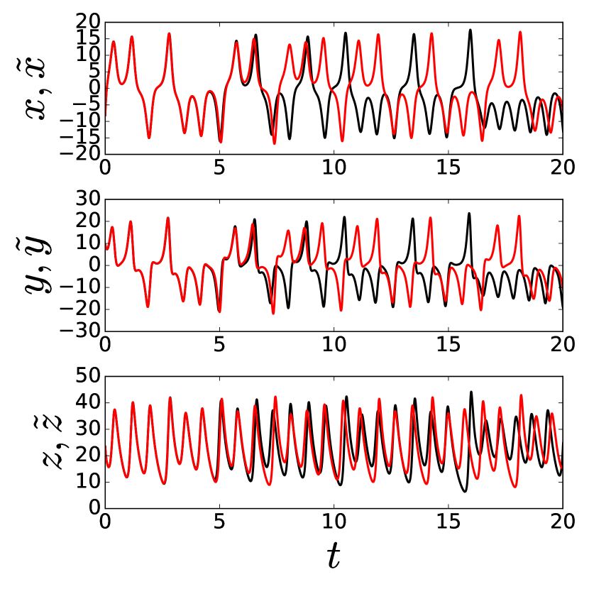
(a) Time series of components

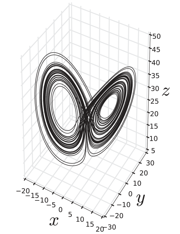
(b) Trajectory presentation in phase space

Figure 1: Illustration of the chaotic dynamics of the Lorenz system (14) with parameter values $\sigma=10$, $\rho=28$ and $\beta=8/3$. (a) Two simulations for the Lorenz system starting from two slightly different initial conditions $(x,y,z)=(-10,10,25)$ and $(\tilde{x},\tilde{y},\tilde{z})=(-10.01,10,25)$. The Lorenz attractor has a positive Lyapunov exponent and the trajectories diverge from each other. (b) Representation of the trajectory of $(x,y,z)=(-10,10,25)$ in the phase space. The shape of the attractor resembles a butterfly.

The Lorenz equations are dissipative and all trajectories eventually enter the absorbing domain

$$\Omega=\left\{\textbf{\em x}\in\mathbb{R}^{3}\,\,:\,\,\rho x^{2}+\sigma y^{2}+\sigma(z-2\rho)^{2}<\frac{\beta^{2}\rho^{2}}{\beta-1}\right\},$$

see Appendix C or Ref. [113]. For the classical parameters, $\sigma=10,\rho=28$ and $\beta=8/3$, inside $\Omega$, trajectory accumulates on the chaotic Lorenz attractor [124], as depicted in Fig. 1(b). Close to the attractor nearby trajectories diverge. To see this, we simulate two trajectories with nearly the same initial condition. The initial $10^{-2}$ difference grows to roughly $10^{2}$ in a matter of only six cycles, see Fig. 1(a). Using numerical simulations, we estimate the maximal divergence rate of nearby trajectories $\Lambda\approx 0.906$.

We consider two coupled chaotic Lorenz oscillators, as in Eq. (6). We derived above that the critical coupling $\alpha_{c}$ for synchronization depends on the Lyapunov exponent $\Lambda$. Using the numerical results for $\Lambda$ we obtain

$$\alpha_{c}=\frac{\Lambda}{2}\approx 0.453.$$

Simulation confirms that this critical coupling is sharp. Indeed, for $\alpha=0.4$ there is no synchronization, and trajectories do not move together, see Fig. 2(a). On the other hand, when $\alpha=0.5$, the trajectories synchronize, see Fig. 2(b)).

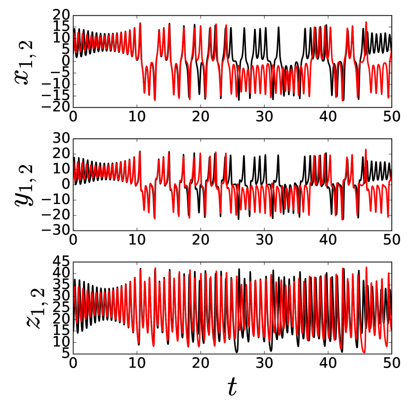
(a) No synchronization

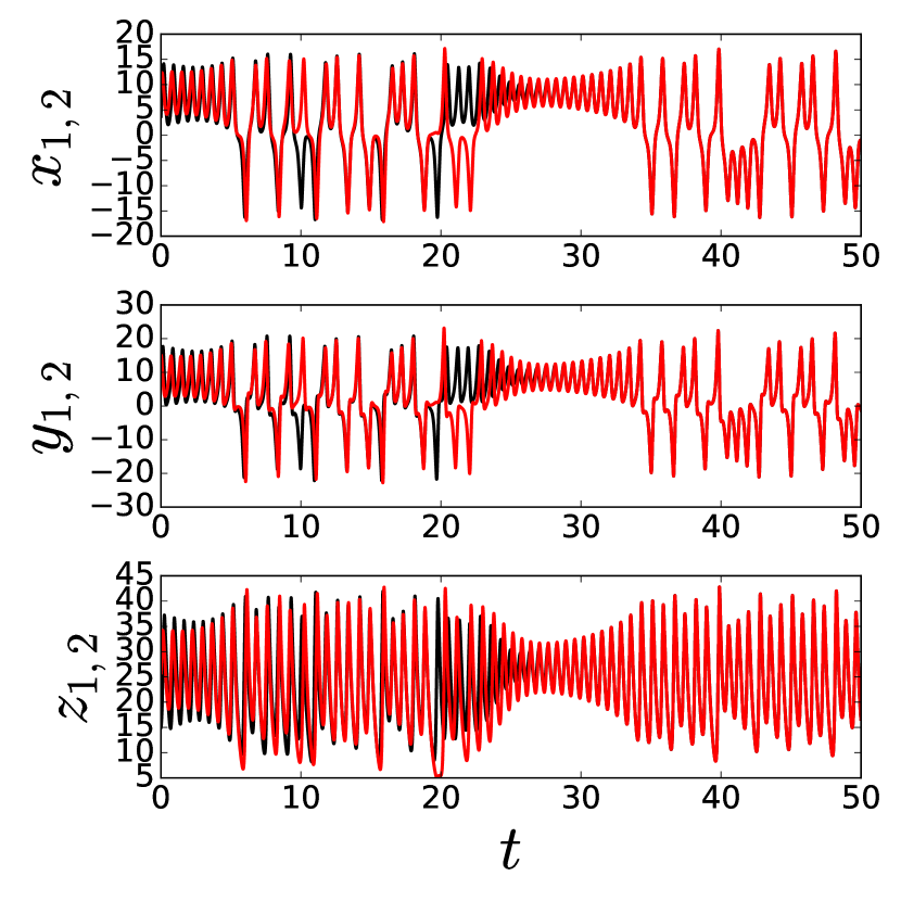
(b) Synchronization

Figure 2: Comparison of trajectories of two initial conditions for the system of two coupled Lorenz systems. The critical transition coupling is $\alpha_{c}\approx 0.453$ for the classical parameters. The initial conditions are selected as $(x_{1},y_{1},z_{1})=(3,10,15)$ and $(x_{2},y_{2},z_{2})=(10,15,25)$. (a) When $\alpha=0.4<\alpha_{c}$, there is no synchronization. (b) If $\alpha=0.5>\alpha_{c}$ one observes synchronization of trajectories.

To compare the amount of synchronization at different parameter values, we may consider the average deviation from synchronization during a time-interval of length $T$ as

$$E=\frac{1}{T}\int_{t=0}^{T}\|\textbf{\em x}_{1}(t)-\textbf{\em x}_{2}(t)\|dt$$ (15)

In Fig. 3(a) we present a synchronization diagram where we plot $E$ against the coupling strength $\alpha$. We observe a good correspondence with the derived value of $\alpha_{c}$. The synchronization error depends on initial conditions so that we compute the synchronization diagram via averaging over some realizations.

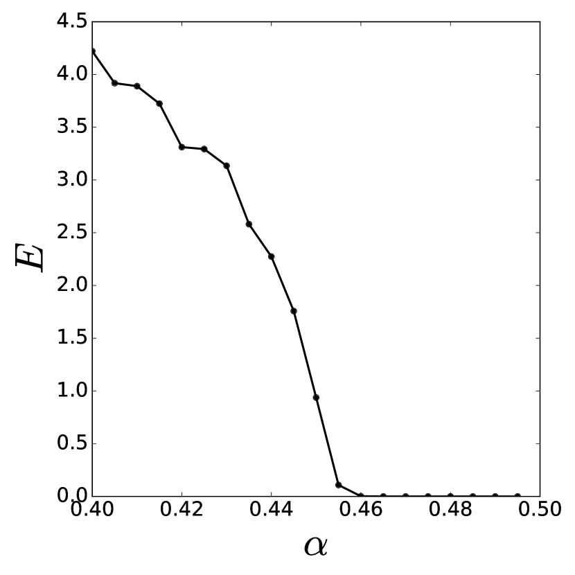
(a) Identity coupling

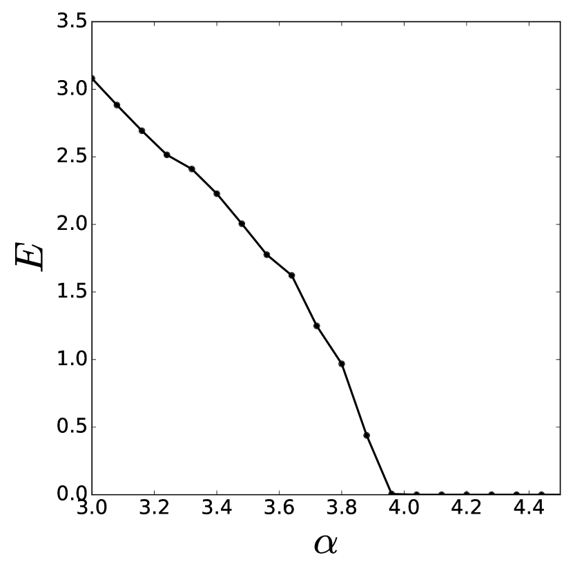
(b) $x$-coupling

Figure 3: Synchronization diagram of two coupled Lorenz systems, (a) with coupling matrix $\textbf{\em H}=\textbf{\em I}$ and (b) with coupling matrix H as in Eq. (16). When $\textbf{\em H}=\textbf{\em I}$, the observed critical coupling constant corresponds to the theoretically derived value $\alpha_{c}\sim 0.453$. With coupling matrix (16), sychronisation is observed to set in for coupling strengths larger than $\sim 3.75$. The synchronization error $E$ was averaged over 300 realisations. Each realisation is simulated by a fourth order Runge-Kutta scheme for 2000 seconds with 0.01 time step.

Examples on different coupling functions. It is worth mentioning that this above analysis works when the coupling adds a damping term $\alpha z$ in other words when $\textbf{\em H}=\textbf{\em I}$. Indeed, the damping term in general form is $\alpha\textbf{\em H}z$ and in this case the above results can no longer be applied. Therefore the synchronization depends on the coupling function, we here just illustrate the effect on synchronization if H is chosen to be

$$\textbf{\em H}=\left(\begin{array}[]{ccc}1&0&0\\ 0&0&0\\ 0&0&0\end{array}\right),$$ (16)

implying that the coupling arises only via the first coordinate $x$. The corresponding synchronization diagram shows that the critical coupling $\alpha_{c}$ for $x$-coupling increases as a result, see Fig. 3(b). Importanly, when H does not commute with the Jacobian matrix along the trajectory, we cannot use the ansatz of Eq. (10). In that case we need a different approach to derive the critical coupling, which will be discussed in Section 4 that deals with synchronization in complex networks.

Rössler System. As a final example, we consider a system introduced by Otto Rössler in 1976:

$$\begin{array}[]{rcl}\dot{x}&=&-y-z,\\ \dot{y}&=&x+ay,\\ \dot{z}&=&b+z(x-c),\end{array}$$ (20)

where $a,b$ and $c$ denote parameters.

We consider two coupled Rössler systems with identity coupling function $\textbf{\em H}=\textbf{\em I}$ and coupling parameter $\alpha$, as in Eq. (6). We consider parameter values $a=0.2$, $b=0.2$ and $c=5.7$. We numerically find that the corresponding attractor has a Lyapunov exponent $\Lambda\approx 0.071$. Hence, the expected critical coupling for synchronization is

$$\alpha_{c}=\frac{\Lambda}{\lambda_{2}}\approx 0.0355$$ (21)

This is in excellent agreement with the numerical results is shown in the synchronization diagram Fig.4.

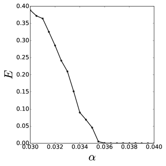
Figure 4: The synchronization diagram of two coupled Rössler systems with the coupling function $\textbf{\em H}=\textbf{\em I}$. The theoretical critical coupling constant $\alpha_{c}\approx 0.0355$ indeed corresponds to the numerically observed one. The synchronization error $E$ was averaged over 300 realisations. Each realisation is simulated by a fourth order Runge-Kutta scheme for 2000 seconds with 0.01 time step.

2.2.1 CS in driven systems

Another possibility is that we use certain sets of variables to drive a subsystem. For appropriate choices we can observe synchronization [85]. We illustrate this scheme in the Lorenz system where $x$-component can be driving signal of another identical system Fig. 5.

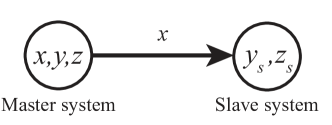
Figure 5: Master-Slave configuration where, $x$-variable is made identical to the response and thereby it drives the response subsystem.

In this scheme we consider the variable $x$ for the master the same as in the slave. That is, the $x$- variable of the master is fully replaced to the $x$ variable in the slave

$$\begin{array}[]{lcc}\dot{x}=\sigma(y-x)&\\ \dot{y}=x(\rho-z)-y&\quad\dot{y_{s}}=x(\rho-z_{s})-y_{s}\\ \dot{z}=-\beta z+xy&\dot{z_{s}}=-\beta z_{s}+xy_{s}\end{array}$$ (25)

where $(x,y,z)$ are the states of the master system and $(y_{s},z_{s})$ are the states of the slave system. In order to check the behaviour of the trajectories, we track the simultaneous variation of the trajectories by $\Delta_{y}(t)=y(t)-y_{s}(t)$ and $\Delta_{z}(t)=z(t)-z_{s}(t)$. For given initial conditions $(x,y,z,y_{s},z_{s})=(-10.1,10.1,10.1,0.1,0.1)$, $\Delta y$ and $\Delta z$ goes to zero (Fig. 6).

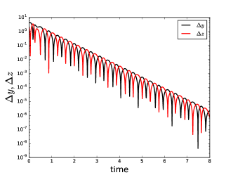
Figure 6: Simulation of master-slave type of coupling

For this particular choice of subsystem it is possible to construct a Lyapunov function for the displacements $\Delta_{y}=y-y_{s}$ and $\Delta_{z}=z-z_{s}$ for $x$-driven system (Eq. (25)).We obtain

$$\begin{array}[]{rcl}\dot{\Delta}_{y}&=&-\Delta_{y}-x\Delta_{z}\\ \dot{\Delta}_{z}&=&x\Delta_{y}-\beta\Delta_{z}.\end{array}$$ (26)

Next consider the Lyapunov function

$$V=\frac{1}{2}\left(\Delta_{y}^{2}+\Delta_{y}^{2}\right),$$

and along solutions of the subsystem we obtain $\dot{V}=\Delta_{y}\dot{\Delta}_{y}+\Delta_{z}\dot{\Delta}_{z}$, after some manupulation we obtain

$$\dot{V}=-\Delta^{2}_{y}-\beta\Delta^{2}_{z}.$$

Since $V$ is positive and $\dot{V}$ negative $\Delta_{y}$ and $\Delta_{z}$ will converge to zero. So, the slave subsystem will have the same dynamics as the master.

2.3 Phase synchronization

If there are small mismatches between the systems another type of synchronization can appear for very small coupling strengths: Phase Synchronization (PS) – which corresponds to a locking of phases of chaotic oscillators

$$|m\phi_{1}(t)-n\phi_{2}(t)|<C$$

where $\phi$ is the phase of the chaotic oscillators, $m,n$ and $C$ are constants. When this holds we have phase synchronization between the two systems [102, 103]. We are considering the phases on the lift, that is, diverging steadily as opposed to consider the phase mod $2\pi$. The phase difference won’t be precisely zero because of the chaotic nature of the system. We could consider higher relations of phase locking, however, the higher the relation $m:n$ more difficult is to observe the phase synchronization. Therefore, our examples will be for $1:1$ phase synchronization.

Phase synchronization is also vast research periodic oscillators [95, 101, 123, 122]. In this case, the phases may be perfectly locked. If we are considering periodic oscillators the phase reduction approach will lead to a description of the interaction in terms of the phases alone [62]. The simplest equation in this setting is

$$\dot{\phi}_{1,2}=\omega_{1,2}+\alpha\sin(\phi_{2,1}-\phi_{1,2})$$

where $\phi$ is the phase along the periodic orbit. Introducing the phase difference $\Phi=\phi_{1}-\phi_{2}$ and $\Delta=\omega_{1}-\omega_{2}$ we obtain

$$\dot{\Phi}=\Delta-2\alpha\sin\Phi$$

this equation has a stable fixed point $\Phi=\phi_{1}-\phi_{2}=$ constant if $\alpha>\alpha_{c}=|\Delta|/2$.

For a chaotic oscillator if coupling strength is small, the amplitudes will remain chaotic but the phase difference will be bounded. Though, it will oscillate as a result of the coupling to the amplitude. In general, it is not straightforward to introduce a phase for a chaotic attractor [53, 96, 91, 10, 9]. For a suitable class of attractors it is possible to define a phase in a useful way.

We focus on coupled two nonidentical Rössler oscillators, the equation is given by

$$\begin{array}[]{rcl}\dot{x}_{1,2}&=&-\omega_{1,2}y_{1,2}-z_{1,2}+\alpha(x_{2,1}-x_{1,2})\\ \dot{y}_{1,2}&=&\omega_{1,2}x_{1,2}+ay_{1,2}\\ \dot{z}_{1,2}&=&b+z_{1,2}(x_{1,2}-c)\end{array}$$ (27)

where $a=0.165$, $b=0.2$ and $c=10$ are the constants of the Rössler system. $\omega$ is the mismatch parameter to make the oscillators nonidentical and given as $\omega_{1,2}=\omega_{0}\pm\Delta$ where $\omega_{0}=0.97$ and $\Delta=0.02$. $\alpha$ is the coupling constant, the system is coupled over $x$ components ($x$-coupling). For certain values of the parameter $a$, the projection of the attractor on $x-y$ plane resembles a limit cycle and the trajectories rotates around the origin (see Fig. 7), and phase and amplitudes are given by

$$\phi_{1,2}=\arctan\left(\frac{y_{1,2}}{x_{1,2}}\right)$$ (28)

$$A_{1,2}=\sqrt{x_{1,2}^{2}+y_{1,2}^{2}}.$$ (29)

We consider the phase on the lift (growing in time without taking the mod).

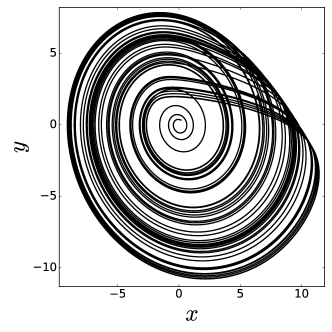
Figure 7: Projection of the Rössler attractor on $x-y$ plane for $a=0.165$.

To gain insight on the adjustment of rhythm leading to phase synchronization, we analyze the average frequencies defined as

$$\Omega_{1,2}=\lim_{T\rightarrow\infty}\frac{\phi_{1,2}{(T)}-\phi_{1,2}(0)}{T}.$$ (30)

And the frequency mismatch is

$$\Delta\Omega=\Omega_{2}-\Omega_{1}$$ (31)

When phase synchronization occurs $|\phi_{1}(t)-\phi_{2}(t)|\leq C,$ the average frequency is the same $\Delta\Omega=0$. The phase difference will not be tend to a constant as the phase nature of the amplitudes acts as a noise in the phases causing mismatches. The comparison of the amplitude difference (Eq. (15)) and the phase (Eq. (31)) is given in Fig. 8. If we increase the coupling constant $\alpha$.

Figure 8: For a weak coupling constant: Although there is no synchrony for the difference of the amplitudes Eq. (15)(top panel), there is a tendency towards to phase synchronization while the coupling constant $\alpha$ increases Eq. (30) (bottom panel). The synchronization error $E$ and frequency mismatch $\Delta\Omega$ were averaged over 300 realisations. Each realisation is simulated by a fourth order Runge-Kutta scheme for 2000 seconds with 0.01 time step.

An approximate theory of phase synchronization can be obtained by averaging [105]. We write the model Eq. (27) in terms of the phase Eqs. (28) as

$$\dot{\phi}_{1,2}=\frac{x_{1,2}\dot{y}_{1,2}-y_{1,2}\dot{x}_{1,2}}{A^{2}}$$ (32)

In this form, using polar coordinates we have $x_{1,2}=A_{1,2}\cos\phi_{1,2}$ and $y_{1,2}=A_{1,2}\sin\phi_{1,2}$, and using this representation in Eq. (32), we obtain

$$\dot{\phi}_{1,2}=\omega_{1,2}+a\sin\phi_{1,2}\cos\phi_{1,2}+\frac{z_{1,2}}{A_{1,2}}\sin\phi_{1,2}-\alpha\left(\frac{A_{2,1}}{A_{1,2}}\cos\phi_{2,1}\sin\phi_{1,2}-\cos\phi_{1,2}\sin\phi_{1,2}\right)$$ (33)

The idea now is that since the mismatch is small, both phases behave nearly the same. So we can split the dynamics of the phases as an overall increasing trend $\omega_{0}t$ and a slow phase dynamics $\theta$. This split is very clear in Fig. 13. So, we write

$$\phi_{1,2}=\omega_{0}t+\theta_{1,2},$$

To obtain an equation for $\theta$ (simpler than the one for $\phi$) we use the fact that $\theta$ is a slow variable. That is, while $\omega_{0}t$ grows a lot $\theta$ is nearly constant. Hence, we will average out the contribution of $\omega_{0}t.$ So we average the phases over $\omega_{0}t$ over a period $\frac{2\pi}{\omega_{0}}$ and keep $\theta_{1,2}$ fixed. After some laborious manipulation we obtain

$$\frac{d}{dt}(\theta_{1}-\theta_{2})=2\Delta-\frac{\alpha}{2}\left(\frac{A_{2}}{A_{1}}+\frac{A_{1}}{A_{2}}\right)\sin(\theta_{1}-\theta_{2})$$ (34)

Both amplitudes $A_{1,2}$ depend on time and display a chaotic behaviour. Lets assume for a moment that they are constant. Then for the phase locking of the Rössler systems, $\frac{d}{dt}(\theta_{1}-\theta_{2})=0$, the equation has a stable fixed point,

$$\theta_{1}-\theta_{2}=\arcsin\frac{4\Delta A_{1}A_{2}}{\alpha(A_{1}^{2}+A_{2}^{2})}.$$ (35)

This fixed point only exists when the argument of the arcsin has modulus less than 1. Therefore, we obtain the critical transition coupling

$$\alpha_{c}\approx 2\Delta.$$

For the given parameters ($\Delta=0.02$) we find $\alpha_{c}\approx 0.04$, in agreement with the numerical analysis Fig. 8. The chaotic behaviour of the amplitudes leads to fluctuations of the phases around the stable fixed point, and so the phases different will not be identically zero. Close to the critical coupling strength the frequencies exhibit a critical behaviour $\Delta\Omega\propto|\alpha-\alpha_{c}|^{1/2}$ as observed observed in Fig. 8.

2.4 Generalized synchronization

When the interacting systems are different, either because of a large parameter mismatch or the systems have distinct dynamics, these two can still exhibit synchronization in a generalized sense. Generalized Synchronization (GS) can be observed in mutually coupled systems as well as unidirectionally coupled system [85, 43, 61, 119]. Surprisingly, GS can be a mapped to a complete synchronization (CS) problem!

Here we will focus on the dynamics of unidirectionally coupled systems. The master x and the slave y systems coupled as

$$\dot{\textbf{\em x}} = \textbf{\em f}(\textbf{\em x})$$

$$\dot{\textbf{\em y}} = \textbf{\em g}(\textbf{\em y},\textbf{\em h}(x))$$ (36)

where $\textbf{\em x}\in\mathbb{R}^{n}$, $\textbf{\em y}\in\mathbb{R}^{m}$ and $\textbf{\em h}(x)$ is the coupling. For certain coupling strengths, the dynamics of system $y$ is totally determined by the dynamics of system $x$. That is, the solutions of, say $x$ can be mapped into solutions of $y$.

$$y=\psi(x)$$

where $\psi$ is a function from the phase space of the system $x$ to the phase space of system $y$. When this happens we have generalized synchronization between these two systems. CS is a particular case of GS when $\psi$ is the identity.

To detect a functional relation between two systems in generalized synchronization, Rulkov and co-workers proposed a technique called mutual false nearest neighbours [104]. The main idea is the see how nearby points are mapped under the dynamics. By studying the properties of nearby points one can infer the existence of the mapping $\psi$. Here, we focus on another approach that turns the GS problem into a CS problem. This is the auxiliary system approach [1, 58]. The master system drives the slave system and an auxiliary system (copy of the slave). If the two copies of the slave exhibit CS then the master and slave are in GS.[1, 58]. An illustration of this scheme can be found in See Fig. 9.

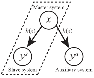
Figure 9: Scheme of the auxiliary system approach for the generalized synchronization. Originally we only have the system in the dashed line box which is master-slave system as in Sec. 2.2.1. Then we add an auxiliary (helper) system $y^{a}$. If there is CS between $y^{s}$ and $y^{a}$, then the GS occurs between x and $\textbf{\em y}^{a,s}$.

Necessary conditions for the occurrence of GS for the system given by Eq. (37) is introduced by Kocarev and Parlitz as following: for all $(\textbf{\em x}_{0},\textbf{\em y}_{0})\in B$, where $\textbf{\em x}_{0}$ and $\textbf{\em y}_{0}$ are states for the master-slave systems at time $t=0$ and $B$ is the basin where all the trajectories approach to a manifold

$$M_{\psi}=\{(\textbf{\em x},\textbf{\em y}):\textbf{\em y}={\psi}(\textbf{\em x})\}.$$

If $M_{\psi}$ is attractive, different trajectories of the slave system will converge to the trajectory lying in $M$ and it is determined only by $x$. In other words, if the master drives a slave $\textbf{\em y}^{s}_{0}$ and an auxiliary (copy of slave) $\textbf{\em y}^{a}_{0}$ systems simultaneously, the driven ones must be completely synchronized $\forall\textbf{\em y}^{s}_{0},\textbf{\em y}^{a}_{0}\in B_{y}$ we have

$$\lim_{t\to\infty}\|\textbf{\em y}^{s}_{t}-\textbf{\em y}^{a}_{t}\|=0.$$

Example: Consider two identical Rössler systems (Eq. (20)) with the parameters ($a=0.2$, $b=0.2$ and $c=5.7$) are driven by a Lorenz system (Eq. (14)) with the classical parameters ($\rho=28,\sigma=10$ and $\beta=8/3$) via $x$-components. We used the auxiliary system approach the detect the critical coupling for GS. Indeed, numerical results showed that $\alpha_{c}\approx 0.12$ as seen in the synchronization diagram Fig. 10. For given $\alpha=0.06$ CS is not observed between the slave systems therefore there is no GS between master and slave systems as well Fig. 11(a). For a coupling constant larger than the critical one $\alpha=0.2$ the slave and the auxiliary system display CS. Hence GS can be observed between master-slave system Fig. 11(b).

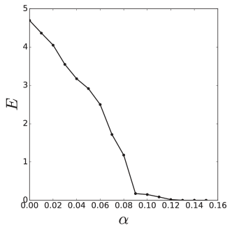
Figure 10: Generalized Synchronization: Averaged over 300 realisations, time=4000 and time step=0.01

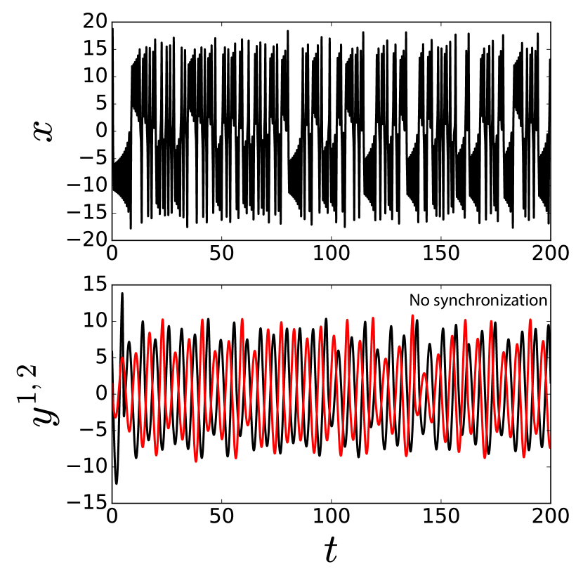
(a) No Synchronization

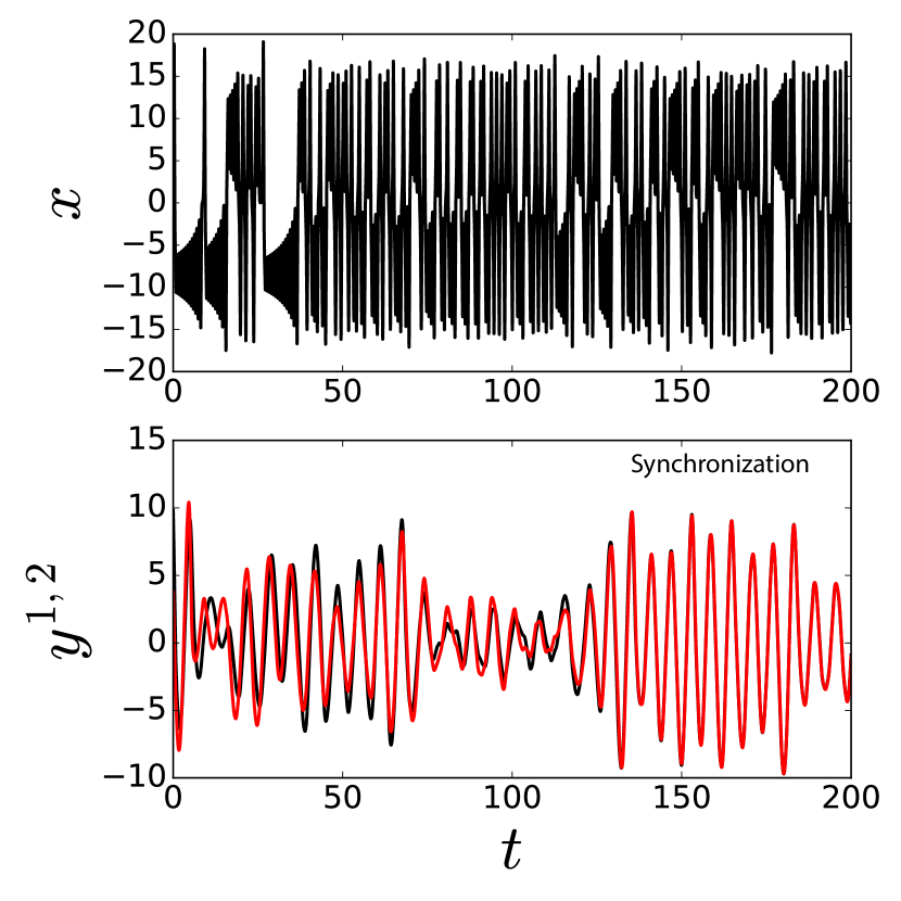
(b) Synchronization

Figure 11: Two simulations for the generalized coupling scheme: a Lorenz system x drives two Rössler systems $\textbf{\em y}^{s,a}$. The critical transition coupling is $\alpha_{c}\approx 0.12$. (a) For the coupling constant $\alpha=0.06$, there is no synchronization since $\alpha<\alpha_{c}$ (b) for $\alpha=0.2$ synchronization is obtained since $\alpha>\alpha_{c}$.

2.4.1 Generalized Synchronization between diffusively coupled oscillators

To gain some insight on this, we will use some ideas put forward by [48, 49]. This approach allows us to obtain a analytical understanding of the critical coupling associated with the transition to GS. Consider a master-slave system diffusively coupled.

$$\dot{\textbf{\em x}} = \textbf{\em f}(\textbf{\em x})$$

$$\dot{\textbf{\em y}} = \textbf{\em g}(\textbf{\em y})+\alpha\textbf{\em H}(x-y)$$ (37)

where H is a positive definite matrix. We can write the slave equation as

$$\dot{\textbf{\em y}}=\bar{\textbf{\em g}}(\textbf{\em y})+\alpha\textbf{\em H}\textbf{\em x}$$

where $\bar{\textbf{\em g}}(\textbf{\em y})=\textbf{\em g}(\textbf{\em y})-\alpha\textbf{\em H}\textbf{\em y}.$ The equation then splits into contributions solely coming from the slave and the driver. Now consider two copies of the slaves $\textbf{\em y}_{1}$ and $\textbf{\em y}_{2}$. Because we know the system will exhibit GS when the copies of the slaves synchronize, we introduce a variable $\textbf{\em z}=\textbf{\em y}_{1}-\textbf{\em y}_{2}$. The system will undergo GS when $\textbf{\em z}\rightarrow\textbf{\em 0}$. Differentiating we obtain

$$\dot{\textbf{\em z}}=\textbf{\em U}(t)\textbf{\em z}-\alpha\textbf{\em H}\textbf{\em z},$$ (38)

where we used the mean value theorem [52] to express

$$\textbf{\em U}(t)\textbf{\em z}=\textbf{\em g}(\textbf{\em y}_{1}(t))-\textbf{\em g}(\textbf{\em y}_{1}(t)+\textbf{\em z}(t))=\left(\int_{0}^{1}D\textbf{\em G}(\textbf{\em y}_{1}(t)+s\textbf{\em y}_{2}(t))ds\right)\textbf{\em z}(t)$$

Notice that for the difference z the driving term Hx disappears as it is common for both copies of the slave $\textbf{\em y}_{1}$ and $\textbf{\em y}_{2}$. The only part of the coupling remaining is the term $-\alpha\textbf{\em H}\textbf{\em z}$, which adds an extra damping and provides dissipation. The trivial solution of z is globally stable if the coupling is large enough. Indeed, we can construct a Lyapunov function for z. Indeed, consider

$$V(\textbf{\em z})=\frac{1}{2}\langle\textbf{\em z},\textbf{\em z}\rangle,$$

and differentiating the Lyapunov function along the solution $\textbf{\em z}(t)$ of Eq. (38) we obtain

$$\frac{dV(\textbf{\em z}(t))}{dt} = \langle\dot{\textbf{\em z}}(t),\textbf{\em z}(t)\rangle$$ (39)

$$\leq (\|D\textbf{\em g}\|-\alpha\lambda_{min}(\textbf{\em H}))\|\textbf{\em y}\|^{2}$$ (40)

where $\lambda_{min}(\textbf{\em H})$ is the minimum eigenvalue of H. In this last passage, we used the Cauchy Schwartz inequality $|\langle\textbf{\em U}(t)\textbf{\em z},\textbf{\em z}\rangle|\leq\|\textbf{\em U}(t)\textbf{\em z}\|\|\textbf{\em z}\|\leq\|\textbf{\em U}\|\|\textbf{\em z}\|^{2}$, and noticed that $\|\textbf{\em U}\|\leq\|D\textbf{\em g}\|$. We also used the fact that H is positive $\langle\textbf{\em H}\textbf{\em z},\textbf{\em z}\rangle\geq\lambda_{min}(\textbf{\em H})\|\textbf{\em z}\|^{2}$. Hence, for

$$\alpha>\alpha_{c}=\frac{\|D\textbf{\em g}\|}{\lambda_{min}(\textbf{\em H})}$$

the derivative of the Lyapunov function is negative and every solution of the system sinks to zero.

What did we learn? When $\alpha>\alpha_{c}$ we have GS. Any two trajectories of the slave $\textbf{\em y}_{1}$ and $\textbf{\em y}_{2}$ will converge towards the same asymptotic state. This happens because the coupling terms adds extra dissipation. The convergence rate is exponential $\|\textbf{\em y}_{1}(t)-\textbf{\em y}_{2}(t)\|\leq Ke^{-\eta t}$ because $\dot{V}\leq\eta V$ and $\eta$ is uniform on the trajectories $\textbf{\em y}_{1},\textbf{\em y}_{2}$ and x. As a conclusion, there a function $\psi$ such that the dynamics of the slave can be as $\textbf{\em y}=\psi(\textbf{\em x})$.

In the literature, a typical way to estimate whether one has GS is to compute the Lyapunov exponents of the slaves. Since we are assuming that the uncoupled systems are chaotic, for $\alpha=0$ the slave will have a positive Lyapunov exponents. As we increase $\alpha$ the maximum Lyapunov exponent may become negative for a value $\alpha_{c}$. We use this $\alpha_{c}$ as an estimate for the critical coupling for GS.

2.5 Summary of Synchronization types

We discuss the three cases commonly found in applications. A schematic representation of the cases is found in Fig. 15.

Complete synchronization in identical systems. If the isolated dynamics are identical, $\textbf{\em f}_{1}=\textbf{\em f}_{2}$ and diffusively coupled, hence, the subspace $\textbf{\em x}_{1}=\textbf{\em x}_{2}$ is invariant under Eq. (6). Indeed, the coupling vanishes and both systems will oscillate in unison for all coupling strengths $\alpha$ and all times. Such collective motion is called complete synchronization (CS). The question is whether CS is attractive, that is, if the oscillators state are nearly the same $\textbf{\em x}_{1}(0)\approx\textbf{\em x}_{2}(0)$, will they synchronize? Meaning that

$$\lim_{t\rightarrow\infty}\|\textbf{\em x}_{1}(t)-\textbf{\em x}_{2}(t)\|=0.$$

See Fig. 12 for an illustration. In Sec 2.2, the CS was discussed in detail.

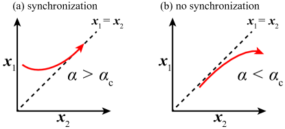
Figure 12: Illustration of complete synchronization. (a) If the coupling strength is large enough ($\alpha>\alpha_{c}$), the systems converge to invariant synchronization manifold ($\textbf{\em x}_{1}=\textbf{\em x}_{2}$), (b) otherwise ($\alpha<\alpha_{c}$), they diverge hence no synchronization.

Phase synchronization (PS) when $\textbf{\em f}_{1}\approx\textbf{\em f}_{2}$. In this situation the subspace $\textbf{\em x}_{1}=\textbf{\em x}_{2}$ is not invariant. And each system will have its own frequency given by their phase dynamics $\phi_{1,2}$. For small coupling strengths the phases can be locked $\phi_{1}\approx\phi_{2}$ while the amplitudes remain uncorrelated Fig. 13. This phenomenon is called phase synchronization. Typically, the critical coupling for PS is proportional to the mismatch $\textbf{\em f}_{1}-\textbf{\em f}_{2}$, as illustrated in Fig. 15. Further details were given in Sec. 2.3.

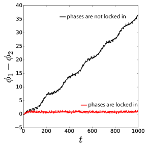
Figure 13: Illustration of phase synchronization for two coupled slightly different and chaotic systems ($\textbf{\em f}_{1}\neq\textbf{\em f}_{2}$). The evolution of the phase differences between the systems for two different coupling constants $\alpha<\alpha_{c}$ and $\alpha>\alpha_{c}$.

Generalized synchronization in master slave configurations. If the vector fields are different $\textbf{\em f}_{1}=\textbf{\em f}$ and $\textbf{\em f}_{2}=\textbf{\em g}$, the systems can synchronize, but in a generalized sense. We consider systems coupled in a master-slave configuration. For certain coupling strengths, the dynamics of the master x can determine the dynamics of the slave y, that is $\textbf{\em y}=\psi(\textbf{\em x})$, see Fig. 14. This is called Generalized Synchronization (GS). Further details for GS was given in Sec. 2.4.

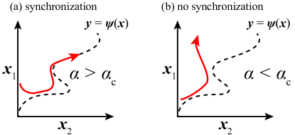
Figure 14: Illustration of generalized synchronization. If the coupling strength is large enough, a functional relationship ($\textbf{\em y}=\psi(\textbf{\em x})$) exhibits between the dynamical variables $\textbf{\em x}_{1}$ and $\textbf{\em x}_{2}$. (a) If $\alpha>\alpha_{c}$, the generalized synchronization is observed (b) otherwise $\alpha<\alpha_{c}$, there is no generalized synchronization.

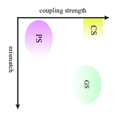
Figure 15: Diagram of synchronization types for diffusively coupled systems. The horizontal axis depicts the mismatch between the isolated dynamics ($\textbf{\em f}_{1}$ and $\textbf{\em f}_{2}$) and the vertical axis the coupling constant. The diagram shows the typical balance between mismatch and coupling strength and to achieve a certain kind of synchronization. Complete synchronization (CS) occurs for identical chaotic systems ($\textbf{\em f}_{1}=\textbf{\em f}_{2}$) and large enough coupling strengths. Phase synchronization (PS) is observed between slightly different systems for small coupling strengths. Generalized synchronization (GS) is a result of master-slave system and can occur for large mismatch parameters or even between distinct systems when the coupling strength large enough.

2.6 Historical Notes

Studies on synchronization dates back to Christiaan Huygens who studied coupled pendulums. In this case, the pendulums are periodic and have distinct frequencies, but due to interaction they adjust their rhythm. In the seventies, thanks to the works of Winfree [127] and Kuramoto [62] the area experienced a boom. In early 2000’s many excellent books and reviews were devoted to this subject [117, 95, 8, 54, 5, 101].

Chaotic synchronization on the other hand is younger. To begin with, the establishment and full acceptance of the chaotic nature of dynamics is fairly new [39]. The role of chaos in nature was object of intense debate in the seventies when Ruelle and Takens proposed that turbulence was generated by chaos.

The chaotic dynamics can be fairly complicated. Typically, the evolution never repeats itself, nearby points drift apart exponentially fast, but in the long run the dynamics return arbitrarily close to its initial state. Such dynamics is so unpredictable that modern approach tackles it from a probabilistic perspective.

Given this complexity many researchers thought it is unlikely one could possibly synchronize two chaotic systems. How could a system with exponential divergence of nearby trajectories have a state were trajectories come together while keeping their chaotic nature? That seemed paradoxal. Chaos and synchronization should not come together. This view was proven wrong in the late eighties. In fact, we have come to think it as rather natural. Funny enough, before this view was accepted synchronization of chaos had to be rediscovered a few times.

Back in the eighties, Fujisaka and Yamada had the first results on synchronization of chaos [37, 130, 131]. They publish it in Japan, but their results went fairly unnotice in the west. Just two years later mathematicians and physicists from Nizhny Novgorod exposed many of the concepts necessary for analyzing synchronous chaos [2]. This paper is now famous, but back then it also went largely unnoticed.

Only some years later the study of synchronization of chaos had its boom, largely as a result of the works by Pecora and Carroll [85]. Lou Pecora and co-workers went systematically tackling two coupled systems and then moved on to study chaotic systems coupled on periodic lattices [44, 20]. These early results were relying on ideas from Nuclear physics to diagonalize the lattice and stability theory (the Lyapunov methods) to analyze synchronization.

The nineties proved prolific for synchronization! Two groups proposed an extension of synchronization, the so-called generalized synchronization [104, 1, 58, 60, 59]. Generalized synchronization only asked for a functional relationship between the states, that is, the dynamics of one system is fully determined by the dynamics of the other. Also in the mid nineties, Rosenblum, Pikovsky and Kurths put forward the concept of chaotic phase synchronization. Here two nearly identical chaotic oscillators can have their phase difference bounded while the amplitudes remain uncorrelated [102, 103].

A few years down the road, Pecora and Carroll were able to generalize their approach to undirected networks of diffusively coupled systems [87]. They also wrote a review about their approach LABEL:ChaosPecora. These results open the door to the understanding of the role of the linking structure on the stability of synchronization. Barahona and Pecora [13] showed that small-world networks are easier to globally synchronize than regular networks. Motter and coworkers [78, 71, 72, 134] showed that heterogeneity in the network structure may hinder global synchronization. On the other hand, Pereira showed such heterogeneity may enhanced synchronization of highly connected nodes [90].

3 Applications

In this section, we discuss the role of synchronization phenomena in various applications including secure communication approaches, parameter estimation of a model from data and prediction.

3.1 Secure Communication based on Complete Synchronization

The first approach is to send an analog message [80]. The key idea is the following: the sender adds the message $m(t)$ on a chaotic signal $x(t)$ and generate a new signal $s(t)=m(t)+x(t)$ (Fig. 16). The assumption is that the amplitude of $x(t)$ is much larger than the amplitude of $m(t)$. This method is called the masking information on bearing signals. Because chaotic signals are noise-like and broadband (have many frequencies), it is difficult to read the message. One could then retrieve the message using synchronization.

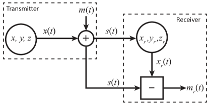
Figure 16: Illustration of the message masking on bearing signal scheme. Transmitter generates a chaotic signal $x(t)$ and add the message $m(t)$ on it. This combined two signals $s(t)=x(t)+m(t)$ is sent to the receiver and both systems synchronize. Discarding the synced signal $x_{r}$ from the $s$, the message $m_{r}\sim m$ is restored.

Masking of messages on bearing signals does not require encryption. Here is the keystone is selection of the transmitter and receiver systems such that they synchronize. They are also assumed to be identical (this means that the receiver knows the parameters of the transmitter). One can retrieve the message if the parameters are known. So, the parameters play a role of encryption key.

We illustrate this communication scheme using the Lorenz system Eq. (14). The Lorenz system has the particularity that it divided into subsystems $(x,z)$ and $(y,z)$. We can use the variables $x$ or $y$ of a subsystem to drive the other subsystem. In this driving setting the synchronization between driver and slave is exponentially stable provided that the parameters $\sigma$, $\rho$ and $\beta$ are identical. Here, we have chosen $x$ component to act as a driver. The message $s(t)$ drives the receiver system as

$$\begin{array}[]{rcl}\dot{x}_{r}&=&\sigma(y_{r}-x_{r})\\ \dot{y}_{r}&=&s(\rho-z_{r})-y_{r}\\ \dot{z}_{r}&=&-\beta z_{r}+sy_{r}.\end{array}$$ (41)

Since the synchronization of chaotic systems is exponentially stable for such system [85, 86] under low amplitude of noise the synchronization (coherence) still occurs. Then the chaotic signal $x_{r}$ can be obtained from Eq. 41. Therefore the message can be regenerated by $m(t)=s(t)-x_{r}(t)$ (Fig. 16).

as a message we use the signal

$$m(t)=0.1\frac{\sin(1.2\pi\sin^{2}(t))}{\pi\sin^{2}(t)}\cos(10\pi\cos{(0.9t)})+\xi$$

where $\xi$ is a white noise Fig. 17(a). We attach this message on $x$-component of the Lorenz system Eq. (LABEL:eq:lorenz_system_app) with parameters $\sigma=16.0$, $\rho=45.2$ and $\beta=4.0$ then the information is masked on bearing signal $s$ Fig. 17(b). By synchronization we restore the message $m_{r}\sim m$ (Fig. 17(c)). This secure communication application is also experimentally demonstrated by using Chua’s circuits [56, 83] and Lorenz-like circuit [26].

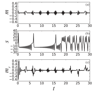
Figure 17: The masking an analog message on bearing chaotic signal. (a) the low-amplitude message, (b) the message embedded into high-amplitude chaotic signal and (c) restored message from the transmitted signal.

The second approach is the modulation of the parameters for the digital communication. In this case, the message $m(t)$ only carries binary-valued signals. The setup is similar to the masking approach but the message is included in the transmitter parameters. The transmitter system has an adjustable parameter $\sigma_{a}(t)=\sigma+\delta m(t)$ such that we can tune the system into synchronization when $m(t)=0$ and out synchronization when $m(t)=1$ Fig. 18. We retrieve the message $m(t)$ by the synchronization and desynchronization pattern.

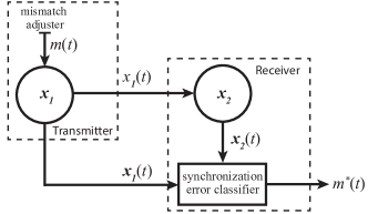
Figure 18: A secure communication scheme: hiding a digital message on a chaotic signal. Changing a parameter of transmitter causes different level of synchronization errors between the transmitter and the receiver. The amplitude of the error $E$ brings the message out.

The dynamics of transmitter and the receiver is given by

$$\dot{x}_{1} = \sigma_{a}(y_{1}-x_{1})$$

$$\dot{y}_{1} = x_{1}(\rho-z_{1})-y_{1}$$

$$\dot{z}_{1} = -\beta z_{1}+x_{1}y_{1}$$

$$\dot{x}_{2} = \sigma(y_{2}-x_{2})$$

$$\dot{y}_{2} = x_{1}(\rho-z_{2})-y_{2}$$

$$\dot{z}_{2} = -\beta z_{2}+x_{1}y_{2}$$

where $\sigma_{a}=\sigma+\delta m(t)$ is the adjustable parameter. Again the key aspect is having mismatch between the transmitter and the receiver does not allow systems to synchronize. Modulating the parameter $\sigma_{a}$ by the message $m(t)$ we can produce different levels of synchronization errors. Choosing the parameters of the transmitter and the receiver identical gives the synchronization error $E\sim$ 0 (CS), this can be assigned binary 0 by $m(t)=0$. The large mismatch $\delta$ causes a certain amount of synchronization error $E>0$, this can be assigned binary signal 1 by $m(t)=1$. Then the digital communication can be set between sender and receiver [25, 26].

Using same parameters as in the previous application ($\sigma=16.0$, $\rho=45.2$ and $\beta=4.0$), we illustrate this digital communication. For this example, a digit of the message is set for 10 time units and the message is 0101010101 (Fig. 19(a)). For each message time, we change $\sigma_{a}$ from $\sigma$ to $\sigma+\delta$ and other way round. Then the synchronization error $E$ varies according to this change (Fig. 19(b)). Due to change in the $E$, the message is restored (Fig. 19(c)).

There are more communication applications using the synchronization mechanism e.g. using hyperchaotic systems [28, 59, 89, 20] or volume-preserving maps [21]. The common idea of all these given approaches is the CS phenomena, negative conditional Lyapunov exponent between the systems are needed to exhibit of the synchronization [85, 86].

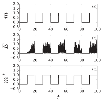
Figure 19: Manipulating the parameter of a transmitter allows digital secure communication. In this application 10 time units are used for a single digit. (a) Digital message (0101010101), (b) the synchronization error and (c) restored message.

3.2 Secure Communication Based on Phase Synchronization

Security is an important issue for communication approaches. As might be expected, some methods were improved and reported to break the CS based communication schemes [94, 109, 29, 84]. Then more secure communication scheme demonstrated by means the PS [22].

The scheme based on the PS possesses three chaotic Rössler systems ($\textbf{\em x}_{1,2,3}$). The transmitter of the scheme consists of two weakly coupled identical systems $\textbf{\em x}_{1}$ and $\textbf{\em x}_{2}$ over their $x$-components Eq. (42) and the receiver $\textbf{\em x}_{3}$ has slightly different dynamics. In this case, we couple the systems with using their phases Eq. (42) as presented in Ref. [23]. The phase definition for Rössler system is given by Eq. (28). The mean of two systems’ phases $\phi_{1}$ and $\phi_{2}$ in transmitter can be used as a spontaneous phase signal $\phi_{m}$ to couple the third system as in Eq. (42). As distinct from the CS based schemes, we have three systems and the reason behind these to improve the security. The return maps of the phase $\phi_{m}$ is way more complex than $\phi_{1}$ (or $\phi_{2}$), this makes to break dynamics not trivial [22].

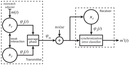
Figure 20: A secure communication scheme by phase synchronization: hiding a digital message on a chaotic signal. Changing a parameter of transmitter causes …

We illustrate this application by

$$\begin{array}[]{rcl}\dot{x}_{1,2}&=&-(\omega+\Delta\omega)y_{1,2}-z_{1,2}+\epsilon(x_{2,1}-x_{1,2})\\ \dot{y}_{1,2}&=&x_{1,2}+ay_{1,2}\\ \dot{z}_{1,2}&=&b+z_{1,2}(x_{1,2}-c)\\ \dot{x}_{3}&=&-y_{3}-z_{3}+\alpha(r_{3}\cos{\phi_{m}}-x_{3})\\ \dot{y}_{3}&=&x_{3}+ay_{3}\\ \dot{z}_{3}&=&b+z_{3}(x_{3}-c)\end{array}$$ (42)

where constant $\omega=1$ and standard parameters of the Rössler system $a=0.15$, $b=0.2$ and $c=10.0$. Coupling constants $\epsilon=5\times 10^{-3}$ is between $\textbf{\em x}_{1}$ and $\textbf{\em x}_{2}$, and $\alpha$ is between the transmitter and the receiver. $r_{3}$ is the amplitude of the response system given by Eq. (29). $\Delta\omega$ is the adjustable mismatch parameter, for this illustration we select

$$\Delta\omega=\left\{\begin{array}[]{ll}0.01&\mbox{if bit digit}=1\\ -0.01&\mbox{if bit digit}=0.\end{array}\right.$$

Similar to digital communication by the CS (see Section 3.1), the modulation of parameters in the transmitter would hide a binary message $m(t)$ on $\phi_{m}$. The PS will exhibit between $\phi_{m}$ and $\phi_{3}$. Due to the changes on the adjustable control parameters $\Delta\omega$, the phase difference between $\phi_{m}$ and $\phi_{3}$ varies. In other words, the phases are locked on different phase shifts. The message can be retrieved from different phase locking values (Fig. 20).

Because of the weak coupling, the CS never occurs Fig. 23(a). Every 10 time unit we switch $\Delta\omega$ parameter to create a digital message $m(t)$ (010101…) Fig. 23(b). The hidden message on chaotic signal can be restored from the receiver using the phase difference between $\phi_{m}$ and $\phi_{3}$. If the message digit is 0, then the phase difference oscillates most time below 0, otherwise above 0 Fig. 23(c). Therefore it is easy to restore associated message $m^{*}$ Fig. 23(d).

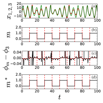
Figure 21: An illustration for the secure communication by phase synchronization: hiding a digital message on a chaotic signal. Changing a parameter of transmitter causes …

In real world examples, it is almost not possible to create identical systems, and the noise is always an issue to deal. The phase locking can be still preservable under effect of a certain level of noise.

3.3 Parameter Estimation and Prediction

Now we have data and we want to learn about the system that generated the data. Thus we will be able to predict the future behaviours and critical transitions. The determining equations of the system are known however the parameters are not. The goal is to find these unknown parameters with using synchronization phenomena. So, we blend the data with equations. The data is then used to drive the equations. If they and coupled in a proper way (Sec. 2.2.1), the equations can synchronize with data. The key point is the following: if the parameters of slave system are identical with the master whose produced driving signal, then the CS exhibits (synchronization error $E=0$) otherwise no CS (synchronization error $E>0$). Therefore, it is possible to estimate the parameters by a strategy to minimize the synchronization error $E\to 0$ such as POWELL technique [97].

We assumed that we have a limited data and we want to predict the future of the system. After the parameters are estimated, the state of the synchronized slave matches the data. Because the solution of the equations are then the same as the data, we can use the equations to predict future dynamics.

The second approach is to estimate a slave system’s parameters of a master-slave system. In this case, the dynamics of master and slave is distinct. We assume that we have two given datasets: one of them from master system and the other one is from the slave. The governing dynamics of the master-slave system is given

$$\dot{\textbf{\em x}} = \textbf{\em f}(\textbf{\em x})$$

$$\dot{\textbf{\em y}} = \textbf{\em g}(\textbf{\em y})+\textbf{\em h}(\textbf{\em x,y})$$

where x and y are the states of master and slave systems respectively. We aim to estimate the parameters of g. Here we cannot use y data to drive another g system directly as in previous approach since y is driven by x. If we know that master-slave system is in the GS and the coupling function $h$ is known, then we can apply the auxiliary system approach which is the master system drives an auxiliary (copy of the slave) z Fig. 22. We expect that the CS exhibits between the slave y and auxiliary z systems if the parameters are identical.

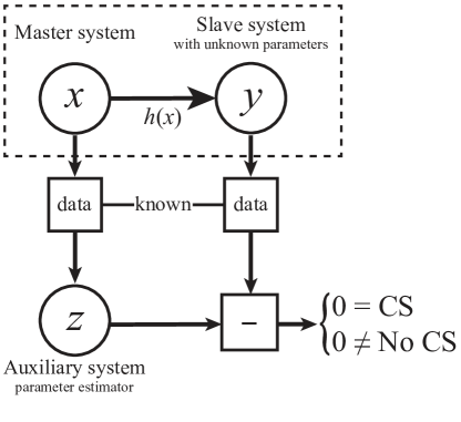
Figure 22: Only two data sets are known from a master-slave system, into the dashed rectangle, without any info about the parameters. An auxiliary system is driven by the data from the master and measure the amplitude difference between the auxiliary and the data from the slave system. If the difference is 0, then there is a CS that means the parameters of the slave and the auxiliary are identical.

Using the GS idea, the problem turned into the CS problem. From now on, minimizing the synchronization error $E\to 0$ technique can be used to estimate the unknown parameters. Similar to the previous approach, the future of the system can be predicted as well.

Example: Consider a Lorenz system with classical parameters is driven by a Rössler system. We have only two data sets, $x_{1}$-component of the Rössler (Eq. (20)) and $y_{1}$-component of the Lorenz (Eq. (14)). Then we drive an auxiliary system z by $x_{1}$ as

$$\dot{z}_{1} = \sigma_{e}(z_{2}-z_{1})+\alpha(x_{1}-z_{1})$$

$$\dot{z}_{2} = z_{1}(\rho_{e}-z_{3})-z_{2}$$

$$\dot{z}_{3} = -\beta_{e}z_{3}+z_{1}z_{2}.$$

The goal is to find the parameters of slave system. The spontaneous synchronization error is

$$E(t)=\|z_{1}-y_{1}\|.$$ (43)

Adjusting the parameters of $\textbf{\em z}(\sigma_{e},\rho_{e},\beta_{e})$ we minimize the simultaneous error $E(t)$ by Powell’s algorithm [97]. This method allows us to estimate the parameters of the slave system (Fig. 23).

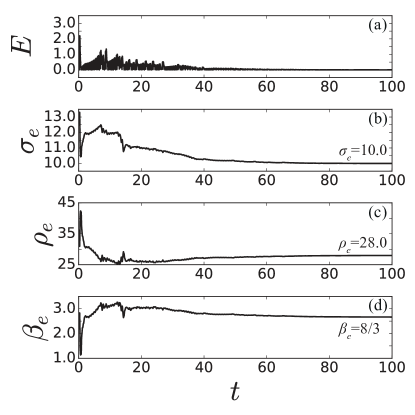
Figure 23: Illustration of parameter estimation estimation. Standard parameters of Lorenz system.

3.4 Chaos Anticipation

Chaos is unpredictable but synchronization can help predicting the state of a chaotic system ahead of time. Anticipating synchronization (AS) is a good approach for the future prediction since the slave system synchronizes with the upcoming states of the master system at time $t+\tau$ where $\tau$ is a time delay. The occurrence of AS depends on the coupling constant $\alpha$. Therefore it is not dependent on isolated dynamics or time delay $\tau$ and regarding to type of desired application higher dimensional chaotic systems can be used for an arbitrary time delay. This anticipation of chaos can be used or is used in applications such as semiconductor lasers with optical feedback, secure communications [66].

Consider two chaotic systems in a master-slave interaction and the master has a certain delay $\tau$ feedback Fig. 24. Because of the internal delay feedbacks, it may well happen that the master x and slave y synchronize but with some time delay

$$\textbf{\em x}(t)=\textbf{\em y}(t-\tau)$$

When this happens we have

$$\textbf{\em y}(t)=x(t+\tau).$$

Hence, although the system $x$ is fully chaotic, we can precisely predict its future state from the system $y$. In other words the slave system anticipates the master system. This kind of synchronization is called anticipated synchronization (AS).

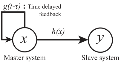
Figure 24: Scheme of anticipating synchronization with memory in the driver systems

Example: We consider two coupled Ikeda equations,

$$\begin{array}[]{rcl}\dot{x}&=&-\alpha x-\mu\sin x_{\tau}\\ \dot{y}&=&-\alpha y-\mu\sin x\end{array}$$ (44)

We use the notation $\textbf{\em y}_{\tau}=\textbf{\em y}(t-\tau)$. The scheme of the system is given in Fig. 24. The synchronization error for delayed system is given by,

$$z=x-y_{\tau}$$

and to show that synchronization is attractive we analyze the first variational equation

$$\dot{z} = \dot{x}-\dot{y}_{\tau}$$ (45)

$$= -\alpha x-\mu\sin x_{\tau}-(-\alpha y_{\tau}-\mu\sin x_{\tau})$$

$$= -\alpha z.$$

The solution is $z(t)=z_{0}e^{-\alpha t}$ and for $\alpha>0$ the synchronization is globally exponentially stable.

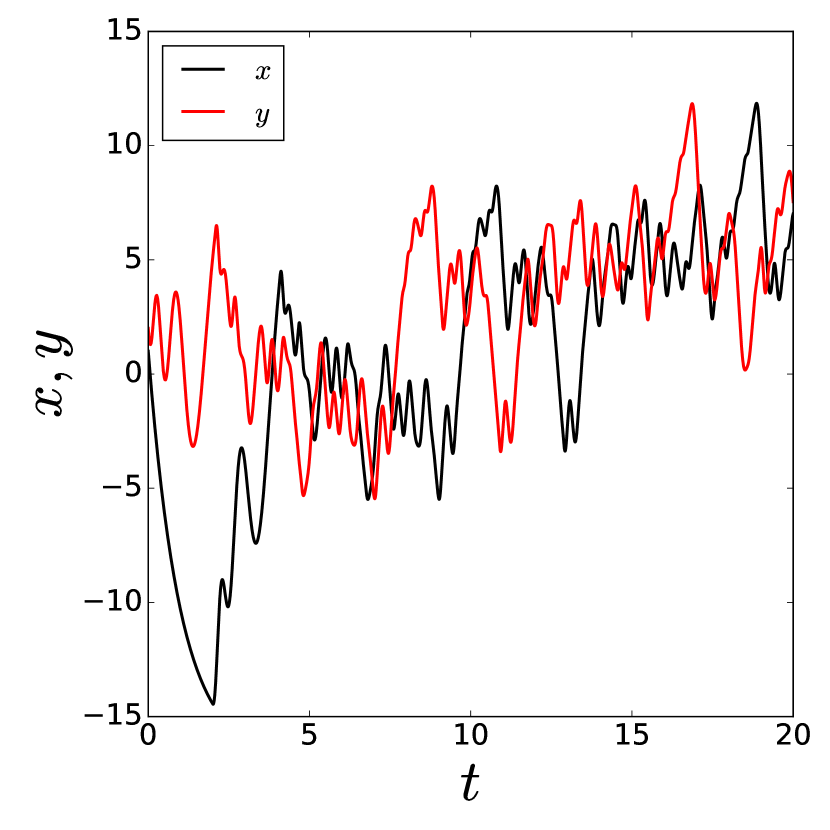
(a) Time series of coupled Ikeda equations.

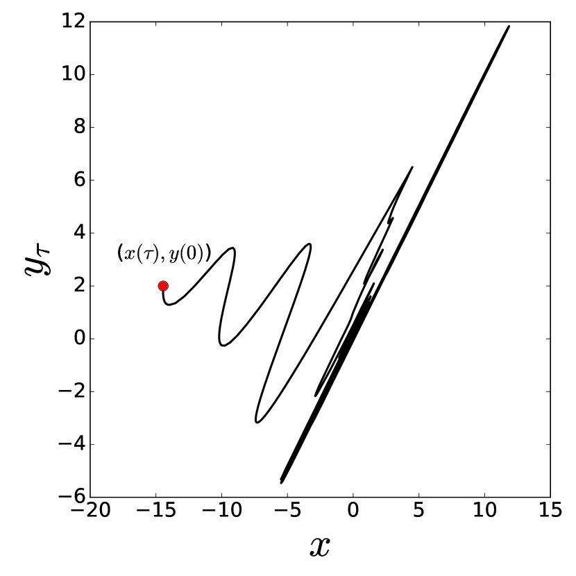
(b) Phase space and synchronization manifold for $x$ and $y_{\tau}$.

Figure 25: Anticipating chaotic synchronization. In the beginning, the systems are not in harmony. After a transient time both systems are getting into a time-delay $\tau$ synchronization. For this illustration $\tau=2$. (a) time series of the systems (b) phase space and synchronization manifold of the system. The red circle is the initial condition for the trajectory of $(x,y_{\tau})$.

To illustrate AS, we simulate Eq. (44) with a fourth order Runge-Kutta integrator for the delay-differential equations for the parameters $\alpha=1$, $\mu=20$ and $\tau=2$. The simulation starts from a random initial condition. After enough transient time $t$, the master $x$ and the slave $y$ systems synchronize with a time delay ($\tau$) Fig. 25(a). The transient time can be observed from the phase space of $x$ and $y_{\tau}$. The initial condition is given by a red circle in Fig. 25(b), the trajectory converges to the synchronization manifold ($\textbf{\em x}=\textbf{\em y}_{\tau}$).

Example: The AS can occur for higher dimensional chaotic system. For such cases the critical coupling constant can be positive ($\alpha_{c}>0$). The AS can be obtained without delayed state in the master system, that is, without memory in the master system. The scheme of this model is given in Fig. 26.

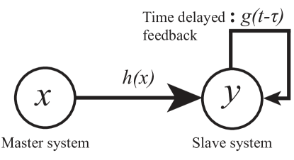
Figure 26: Scheme of anticipating synchronization without memory in the driver systems

We can demonstrate this case with Rössler system, the governing equations are given by

$$\begin{array}[]{rcl}\dot{x}_{1}&=&-x_{2}-x_{3}\\ \dot{x}_{2}&=&x_{1}+ax_{2}\\ \dot{x}_{3}&=&b+x_{3}(x_{1}-c)\\ \dot{y}_{1}&=&-y_{2}-y_{3}+\alpha(x_{1}-y_{1,\tau})\\ \dot{y}_{2}&=&y_{1}+ay_{2}\\ \dot{y}_{3}&=&b+y_{3}(y_{1}-c)\end{array}$$ (52)

where the parameters are $a=0.15$, $b=0.2$ and $c=10$. We simulate Eq. (52) for no AS ($\alpha<\alpha_{c}$) Fig. 27 and AS ($\alpha>\alpha_{c}$) Fig. 27 cases. In this memoryless AS approach, the synchronization is also dependent on time delay $\tau$.

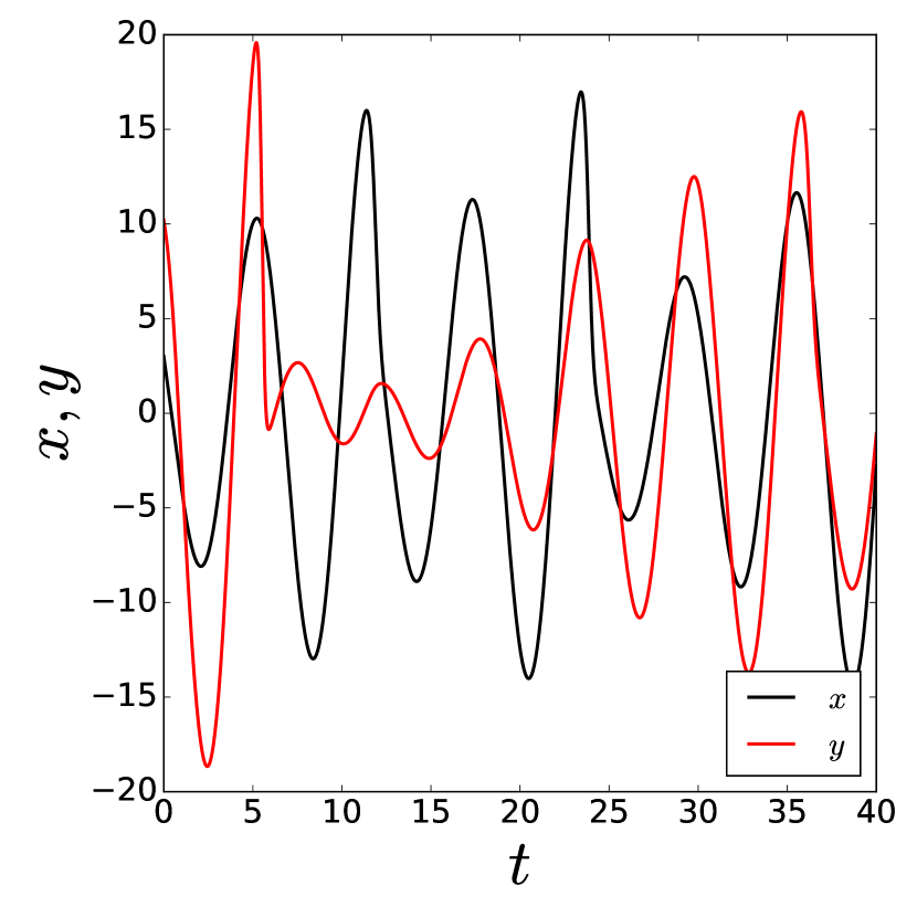
(a) Time series, no synchronization $\alpha<\alpha_{c}$

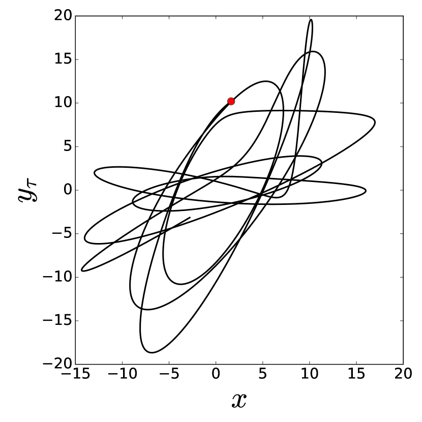
(b) Phase space for $x$ and $y_{\tau}$.

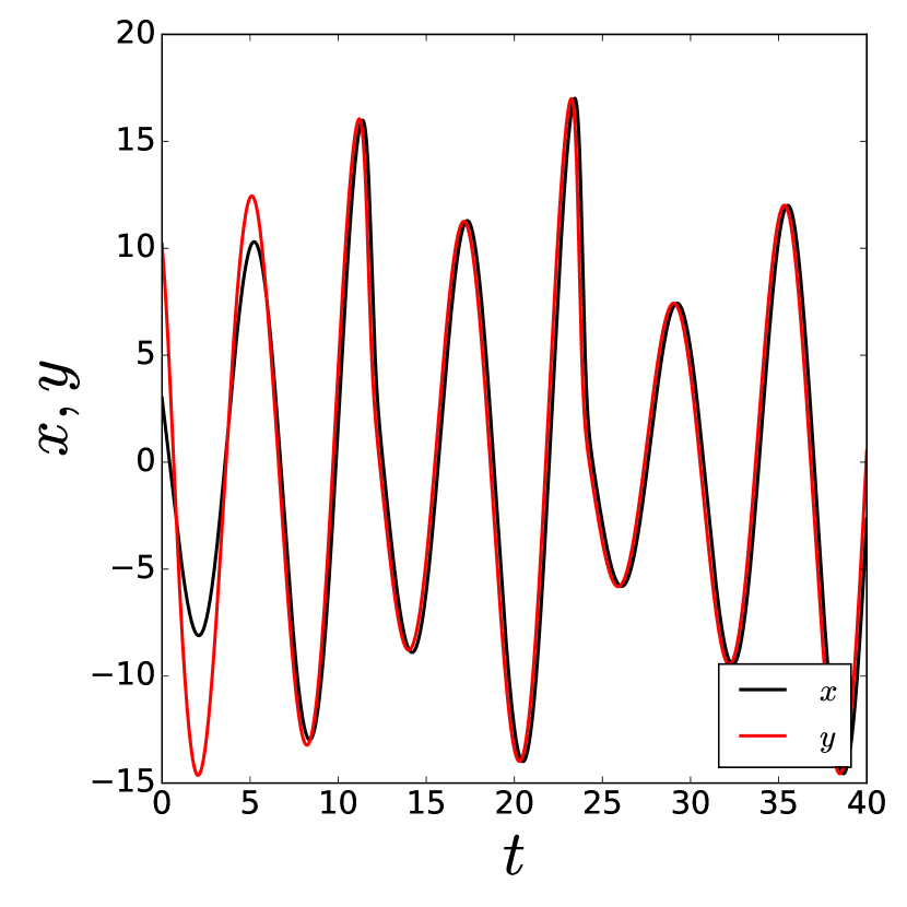
(c) Time series, synchronization $\alpha>\alpha_{c}$

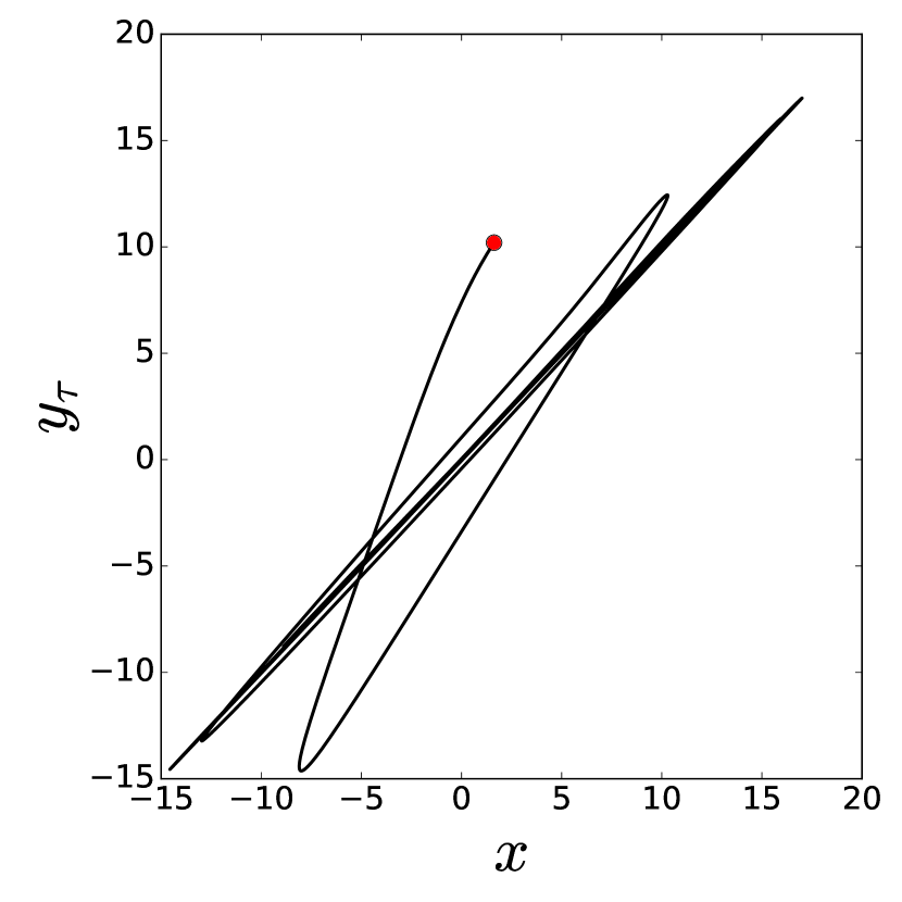
(d) Phase space and synchronization
manifold for $x$ and $y_{\tau}$.

Figure 27: Anticipating synchronization does not obtain for ($\alpha<\alpha_{c}$), otherwise ($\alpha>\alpha_{c}$) the AS exhibits. For this illustration the delay is selected as $\tau=0.2$. (a) time series of the systems where $\alpha<\alpha_{c}$ and (b) phase space. (c) time series of the systems where $\alpha>\alpha_{c}$ and (d) phase space and synchronization manifold of the system. The red circle is the initial condition for the trajectory of $(x,y_{\tau})$.

4 Synchronization in complex networks

Synchronization is commonly found in networks of natural and mankind-made systems such as neural dynamics [110, 15, 40], cardiovascular systems [64, 116, 108], power grids [70], superconducting Joseph junctions [125]. The theory we presented in the previous chapters can be generalized to understand certain aspects of synchronization in these complex systems.

We will focus on diffusively interacting identical oscillators, so the dynamics of the coupled system reads as

$$\frac{d\textbf{\em x}_{i}}{dt} = \textbf{\em f}(\textbf{\em x}_{i})+\alpha\sum_{j=1}^{N}A_{ij}[\textbf{\em H}(\textbf{\em x}_{j})-\textbf{\em H}(\textbf{\em x}_{i})],$$ (53)

where $\textbf{\em f}:\mathbb{R}^{n}\rightarrow\mathbb{R}^{n}$ describes the dynamics of the isolated system, $\alpha$ is the overall coupling strength, $N$ is the number of oscillators, $\textbf{\em H}:\mathbb{R}^{n}\rightarrow\mathbb{R}^{n}$ is the coupling function. Finally, $A_{ij}$ dictates who is interacting with whom. $A_{ij}=1$ if $i$ receives a connection from $j$ and $0$ otherwise. The matrix $A$ (the dimension is $N\times N$) provides the network linking structure and it is called adjacency matrix. This matrix will play an clear role in the analysis.

The network dynamics of diffusively coupled system in Eq. (Electronic Circuits with Resistive interaction.) models many physical systems. A few specific examples are:

Electronic Circuits with Resistive interaction.

Electric circuits, e.g., Chua, Roessler-like, Lorenz-like, can be coupled over their resistors then Eq. models this system [85]. Another case, only one electric circuit can be driven by an external signal as master-slave system (for details, see Sec. 2.2.1)[11].

Neuron Networks with Electrical Coupling.

In brain network, f can be the isolated neuron dynamics modelled by differential equations with chaotic or periodic behaviour and having different time-scales, that is, the isolated can have burst and single regime [47] and $H$ the electrical synapses $H(\textbf{\em x}_{1}-\textbf{\em x}_{2})=(x_{1}-x_{2},0,0)$.

Stable Biological System.

In biological systems when the isolated dynamics has a stable periodic motion then typically one can rephrase the network dynamics in terms of our model. For instance, the heart consists of millions of pacemaker cells. Each cell when isolated has its own rhythm, but when put together these cells interact and behave in unison to deliver the strong electrical pulse that make our heart beat [117]. The dynamics of the pacemaker cells are modelled by phase oscillators $\phi_{i}$ with distinct frequencies $\omega_{i}$ and the coupling function is a simple sine function $H(\phi_{1}-\phi_{2})=sin(\phi_{1}-\phi_{2})$[106, 108].

Laser Arrays.

Lasers can be arranged arrays or complex networks. In this case, one is interested in the electrical field dynamics. Such electrical field is govern by equations with interaction akin to diffusion Ref. [73]. So, the approach presented here can be extrapolated to such lasers under slight changes.

In fact, when we considering periodic oscillators the above model is a normal form for the networked system. That is, the isolated system has a periodic exponentially attracting orbit, we couple the system, and in the weak coupling regime, the amplitudes will change only slightly but the phases can change by large amounts. So the dynamics can be described only in terms of the phases. The phase description will again fit in our Eq. (Electronic Circuits with Resistive interaction.).

Our synchronization results given in the previous sections are exponentially stable. In other words, if once the trajectories are into the synchronization subset, the solution is robust and persistent to the perturbations. For $N$ coupled nonidentical systems ($\textbf{\em f}_{1}\neq\textbf{\em f}_{2}\neq\dots\neq\textbf{\em f}_{N}$), complete synchronization is not possible. However, because of exponentially stable solutions, highly coherent state around the synchronization subset can be still observed [120, 93].

4.1 Interactions in terms of Laplacian

Because of the diffusive nature of the interaction, it is possible to represent the coupling in terms of the Laplacian matrix L. Indeed,

$$\sum_{j=1}^{N}A_{ij}[\textbf{\em H}(\textbf{\em x}_{j})-\textbf{\em H}(\textbf{\em x}_{i})] = \sum_{j=1}^{N}A_{ij}\textbf{\em H}(\textbf{\em x}_{j})-\textbf{\em H}(\textbf{\em x}_{i})\sum_{j=1}^{N}A_{ij}$$

$$= \sum_{j=1}^{N}A_{ij}\textbf{\em H}(\textbf{\em x}_{j})-k_{i}\textbf{\em H}(\textbf{\em x}_{i})$$

$$= \sum_{j=1}^{N}(A_{ij}-\delta_{ij}k_{i})\textbf{\em H}(\textbf{\em x}_{j})$$

where $k_{i}=\sum_{j=1}^{N}A_{ij}$ is the degree of the $i$th node, $\delta_{ij}$ is the Kronecker delta, and recalling that $L_{ij}=\delta_{ij}k_{i}-A_{ij}$ we obtain

$$\frac{d\textbf{\em x}_{i}}{dt} = \textbf{\em f}(\textbf{\em x}_{i})-\alpha\sum_{j=1}^{N}L_{ij}\textbf{\em H}(\textbf{\em x}_{j}).$$ (54)

Our results will depend on this representation and on the spectral properties of L.

Notice that

$$\textbf{\em x}_{1}(t)=\textbf{\em x}_{2}(t)=\cdots=\textbf{\em x}_{N}(t)=\textbf{\em s}(t),$$

is an invariant state for all coupling strength $\alpha$, because the laplacian is zero row sum. When $\alpha=0$ the oscillators are decoupled, and Eq. (64) describes $N$ copies of the same oscillator with distinct initial conditions. Since, the chaotic behavior leads to a divergence of nearby trajectories, without coupling, any small perturbation on the globally synchronized motion will grow exponentially fast, and lead to distinct behavior between the node dynamics. We wish to address the local stability of the globally synchronized state. That is, if all trajectories start close together would become synchronized

$$\lim_{t\rightarrow\infty}\|\textbf{\em x}_{i}(t)-\textbf{\em x}_{j}(t)\|=0$$

The goal of the remaining exposition is to answer this question. Before, we continue with the analysis, we will briefly review some examples and constructions of graphs and discuss the relevant aspects necessary to tackle for problem.

4.2 Relation to other types of Synchronization

We will focus on the transition to complete synchronization, which is mainly related to Sec. 2.2. This is no severe restriction as in certain scenarios other types of synchronization can often be formulated in terms of our model.

Extension to Phase Synchronization. As we discussed in the introduction of Sec. 4, if the dynamics of f is periodic then we can introduce a phase variable which will follow our main system of equations Eq. (Electronic Circuits with Resistive interaction.) as the phase reduction tells us that generically the interaction between phases are diffusive. Moreover, because our results will yield robust transition to synchronization, if the oscillators are nearly identical the phase synchronization will persist.

Extension to Generalized Synchronization. Roughy speaking a form of generalized synchronization in networks is the so-called pinning control, where one tries to control the behaviour of synchronized trajectories by driving the network with external nodes. One extends the network to include the driver node. Therefore, the theory necessary to tackle this problem is the same as presented here. The main question is how to connect the driver nodes in such a way that control is effective.

4.3 Complex Networks

A network, also called graph $G$ in mathematical literature, is a set of $N$ elements, called nodes (or vertices), connected by a set of $M$ links (or edges) Fig. 28. Networks represent interacting elements and are all around from biological systems, e.g. swarm of fireflies, food webs or brain networks, to mankind made systems, e.g. the world wide web, power grids, transportation networks or social networks.

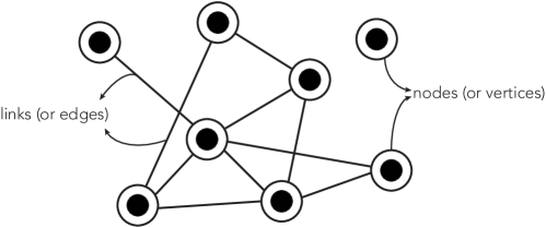
Figure 28: A network visualisation with eight nodes and ten links.

A network is called simple

if the nodes do not have self-loops (i.e., nodes have connections to themselfs). An illustration of a simple network is found in Fig. 29(a). A nonsimple network, therefore, containing connections is depicted in Fig. 29(d). We need a bit of technology from graph theory to make sense of our networks. A few basic notions are as follows

A network is undirected

if there is no distinction between the two nodes associated with each link Fig. 29(a).

A path in a network

is a route (sequence of edges) between connected nodes without repeating i.e. a path can visit a node only once. The length of a path is the number of links in the path. See further details in Ref. [19, 76]. In Fig. 30 we illustrate the paths of two selected (red) nodes in a network. Between two red nodes there are five different paths and each path is given in subplots of Fig. 30. The length of paths are five for Fig. 30(a), four for Fig. 30(b), three for Fig. 30(c) and (d), and two for Fig. 30(e). Therefore the shortest path length, also called geodesic path, between these two red nodes is illustrated in Fig. 30(e).

The network diameter $d$

is the longest length of the shortest path between all possible pairs of nodes. In order to compute the diameter of a graph, first we find the shortest path between each pair of nodes. The longest length of all these geodesic paths is the diameter of the graph. If there is an isolated node (a node without any connections) or disconnected network components, then the diameter of the network is infinite. A network of finite diameter is called connected (Fig. 29(a)), otherwise disconnected (Fig. 29(b)).

A network is directed

if the links transmit the information towards only associated direction Fig. 29(c). If the graph is directed then there are two connected nodes say, $u$ and $v$, such that $u$ reachable from $v$, but $v$ is not reachable from $u$. See Fig. 29(c) for an illustration.

A network is weighted

if links have different importance from each other or the links may be carry different amount of information. Such graphs are called weighted networks Fig. 29(d). Moreover, a network may have self-loops, that is, a node can affect itself as well Fig. 29(d).

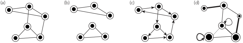
Figure 29: Visualization of network types: (a) an unweighted simple network, (b) a disconnected network, (c) a directed network, (d) a weighted network with self-loops.

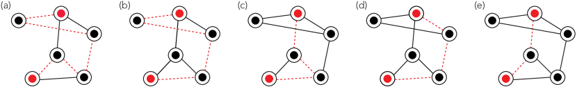
Figure 30: Visualization of paths (red dashed) between two selected nodes (red) in a network: path length of (a) is five, (b) is four, (c) and (d) are three and (e) is two. Therefore the shortest path length for these two red nodes is two.

A graph can be described by its adjacency matrix A with $N\times N$ elements $A_{ij}$. The adjacency matrix A encodes the topological information, and is defined as $A_{ij}=1$ if $i$ and $j$ are connected, otherwise $0$. Therefore, the adjacency matrix of an undirected network is symmetric, $A_{ij}=A_{ji}$. The degree $k_{i}$ of the $i$th node is the number of edges belongs to the node, defined as

$$k_{i}=\sum_{j}A_{ij}.$$

The Laplacian matrix L is another way to represent the network, defined as

$$L_{ij}=\left\{\begin{array}[]{ll}k_{i}&\mbox{if }i=j\\ -1&\mbox{if }i\mbox{ and }j\mbox{ are connected}\\ 0&\mbox{otherwise }.\end{array}\right.$$ (55)

There is a direct relationship between the Laplacian L and the adjacency matrix A. In a compact form it reads

$$L_{ij}=\delta_{ij}k_{i}-A_{ij}$$

where $\delta_{ij}$ is the Kronecker delta, which is 1 if $i=j$ and 0 otherwise. We demonstrate some example network sketches with their adjacency A and Laplacian L matrices in Fig. 31.

complete graph	$\textbf{\em A}=\left(\begin{array}[]{cccccc}0&1&1&1&1&1\\ 1&0&1&1&1&1\\ 1&1&0&1&1&1\\ 1&1&1&0&1&1\\ 1&1&1&1&0&1\\ 1&1&1&1&1&0\end{array}\right)$	$\textbf{\em L}=\left(\begin{array}[]{cccccc}5&-1&-1&-1&-1&-1\\ -1&5&-1&-1&-1&-1\\ -1&-1&5&-1&-1&-1\\ -1&-1&-1&5&-1&-1\\ -1&-1&-1&-1&5&-1\\ -1&-1&-1&-1&-1&5\end{array}\right)$
ring (cycle) graph	$\textbf{\em A}=\left(\begin{array}[]{cccccc}0&1&0&0&0&1\\ 1&0&1&0&0&0\\ 0&1&0&1&0&0\\ 0&0&1&0&1&0\\ 0&0&0&1&0&1\\ 1&0&0&0&1&0\end{array}\right)$	$\textbf{\em L}=\left(\begin{array}[]{cccccc}2&-1&0&0&0&-1\\ -1&2&-1&0&0&0\\ 0&-1&2&-1&0&0\\ 0&0&-1&2&-1&0\\ 0&0&0&-1&2&-1\\ -1&0&0&0&-1&2\end{array}\right)$
star graph	$\textbf{\em A}=\left(\begin{array}[]{cccccc}0&1&1&1&1&1\\ 1&0&0&0&0&0\\ 1&0&0&0&0&0\\ 1&0&0&0&0&0\\ 1&0&0&0&0&0\\ 1&0&0&0&0&0\end{array}\right)$	$\textbf{\em L}=\left(\begin{array}[]{cccccc}5&-1&-1&-1&-1&-1\\ -1&1&0&0&0&0\\ -1&0&1&0&0&0\\ -1&0&0&1&0&0\\ -1&0&0&0&1&0\\ -1&0&0&0&0&1\end{array}\right)$

Figure 31: Various network examples with six nodes. Their adjacency A and Laplacian L matrices.

The networks we encounter in real applications have a wilder connection structure. Typical examples are cortical networks, the Internet, power grids and metabolic networks [76, 75]. These networks don’t have a regular structure of connections such as the ones presented in Fig. 31. We say that the network is complex if it does not possess a regular connectivity structure.

One of the goals is the understand the relation between the topological organization of the network and its relation functioning such as its collective motion.

2$k$ Regular Graph

is a standard graph model where each node has $2k$ links then the total number of links is $M=kN$ where $N$ is total number of nodes Fig. 32 (a). This model is rather important one since the connections of spatiotemporal graphs, in general, connected to the nearest neighbours. $2k$ regular graph is an alternative representation of such models. It is important to mention that the graph model is fixed with given $k$ and $N$ therefore all properties of the graph is known analytically.

Erdös-Rényi

network is generated by setting an edge between each pair of nodes with equal probability $p$, independently of the other edges Fig. 33 (a). If $p\gg\ln N/N$, then a the network is almost surely connected, that is, as $N$ tends to infinity, the probability that a graph on $n$ vertices is connected tends to $1$. The degree is pretty homogeneous, almost surely every node has the same expected degree [24].

Small World

network is a random graph model which possesses the small-world properties; i.e the average path length is short and clustering is large. The network is generated from a $2k$ regular graph, each link of the graph is rewired with a probability $p$. Therefore if $p=0$ then the there is no rewiring and the graph is $2k$ regular. For $p=1$ then each link is rewired i.e the graph is approaching to Erdös-Rényi network with $p=\frac{kN}{2\binom{N}{2}}$. The small-world properties come true between $0<p<1$ Fig. 32. In many real world networks, the properties of small-world topology can be obtained.

(a) 2k-regular graph

(b) Small-World

(c) Random (Erdös-Renyi)

Figure 32: Watts - Strogatz random network approach

The Barabasi-Albert

network possesses a great deal of heterogeneity in the node’s degree, while most nodes have only a few connections, some nodes, termed hubs, have many connections Fig. 33 (a). These networks do not arise by chance alone. The network is generated by means of the cumulative advantage principle – the rich gets richer. According to this process, a node with many links will have a higher probability to establish new connections than a regular node. The number of nodes of degree $k$ is proportional to $k^{-\beta}$. These networks are called scale-free networks [76, 75]. Many graphs arising in various real world networks display similar structure as the Barabasi-Albert network [12, 4, 3].

(a) Barabasi-Albert network

(b) Hypercube network

Figure 33: Some examples of complex networks.

Hypercube graph

$Q_{m}$ is a $m$-dimensional hypercube formed regular graph (Fig. 33 (b)). It is a regular graph since each node has $m$ neighbours and total number of nodes is $2^{m}$ and edges is $2^{m-1}$.

Random networks serve as a proxy to many applications as well as a surrogate. There are many nice ways to construct random network

Configuration Model

is a random network model created by the degree distribution $P(k)$. If the degree distribution of a graph is known, then the nodes with associated number of links are known however the connection structure between nodes is unknown. The nodes can be drawn with their stubs (half links) Fig. 34 (a), then randomly these stubs can be linked and two stubs create a proper link Fig. 34 (b). This process is a random matching, obviously different network structures can arise from this random process.

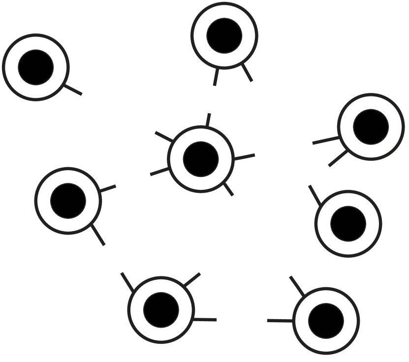
(a) stubs with associated nodes

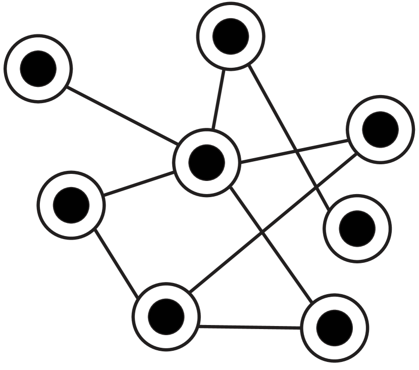
(b) randomly matched stubs

Figure 34: Configuration model.

Expected degrees.

Fix a network of $N$ nodes and consider a vector

$${\textbf{\em w}}=(w_{1},w_{2},\cdots,w_{N}),$$

In this model, each link $A_{ij}$ between nodes $i$ and $j$ is an independent Bernoulli variable taking value $1$ with success probability

$$p_{ij}=w_{i}w_{j}\rho,$$

and 0 with probability $1-p_{ij}$, where

$$\rho=\frac{1}{\sum_{i=1}^{N}w_{i}}.$$

To ensure that $p_{ij}\leq 1$ it assumed that $\textbf{\em w}=\textbf{\em w}(N)$ is chosen so that

$$\Delta^{2}\rho\leq 1.$$ (56)

The degree $k_{i}=\sum_{j}A_{ij}$ of the $i$th is a random variable. An interesting property of this model is that under this construction $w_{i}$ is the expected value of $k_{i}$, that is,

$$\mathbb{E}_{\textbf{\em w}}(k_{i})=\sum_{j}\mathbb{E}_{\textbf{\em w}}(A_{ij})=w_{i}$$

So, the different to the configuration model is that we do not fix the node degree, but rather obtain the degree probabilistically. This model also have many desirable concentration properties in the large $N$ limit.

4.4 Spectral Properties of the Laplacian

The eigenvalues and eigenvectors of A and L tell us a lot about the network structure. The eigenvalues of L for instance are related to how well connected is the graph and how fast a random walk on the graph could spread. In particular, the smallest nonzero eigenvalue of L will determine the synchronization properties of the network. Since the graph is undirected the matrix L is symmetric its eigenvalues are real, and L has a complete set of orthonormal eigenvectors LABEL:LA:ThmDiag. The next result characterizes important properties of the Laplacian

Theorem 1.

Let $G$ be an undirected network and L its associated Laplacian. Then:

• L has only real eigenvalues,

• $0$ is an eigenvalue and a corresponding eigenvector is $\textbf{\em 1}=(1,1,\cdots,1)^{*}$, where ^∗ stands for the transpose.

• L is positive semidefinite, its eigenvalues enumerated in increasing order and repeated according to their multiplicity satisfy

  $$0=\lambda_{1}\leq\lambda_{2}\leq\cdots\leq\lambda_{N}$$

• The multiplicity of $0$ as an eigenvalue of L equals the number of connect components of G.

Therefore, $\lambda_{2}$ is bounded away from zero whenever the network is connected. The smallest non-zero eigenvalue is known as algebraic connectivity, and it is often called the Fiedler value. The spectrum of the Laplacian is also related to some other topological invariants. One of the most interesting connections is its relation to the diameter, size and degrees.

Theorem 2.

Let $G$ be a simple network of size $N$ and $L$ its associated Laplacian. Then:

1. [67] $\lambda_{2}\geq\displaystyle\frac{4}{Nd}$

3. [35] $\lambda_{2}\leq\displaystyle\frac{N}{N-1}k_{1}$

We will not present the proof of the Theorem here, however, they can be found in references we provide in the theorem. We suggest the reader to see further bounds on the spectrum of the Laplacian in Ref. [68]. Also Ref. [69] presents many applications of the Laplacian eigenvalues to diverse problems. One of the main goals in spectral graph theory is the obtain better bounds by having access to further information on the graphs.

For a fixed network size, the magnitude of $\lambda_{2}$ reflects how well connected is graph.

Table 1: Network of $N$ nodes with $m$ mean degree. Examples of nonrandom networks are depicted in Fig. 31 and random networks in Fig. 33. For random networks, the mean degree is given by $m=\sum_{k}kP(k)$ where $P(k)$ is the degree distribution of the network. The randomness of the networks arises via probability $p$. Consider the degree distribution for the SF network $P(k)=k^{-\gamma}$. $C$ is constant.

Network	$\lambda_{2}$	$\lambda_{N}$	$k_{\max}$	$k_{\min}$	$d$	Reference
complete	$N$	N	$N-1$	$N-1$	$1$
ring	$\displaystyle 2-2\cos\left(\frac{2\pi}{N}\right)$	$4$	$2$	$2$	$\begin{array}[]{c}(N+1)/2\mbox{ if $N$ is odd}\\ N/2\,\,\mbox{ \, \, \, \, if $N$ is even}\\ \end{array}$	[5]
star	$\displaystyle 1$	$N$	$N-1$	$1$	2
hypercube (Qm)	$2$	$\frac{2\ln(N-2)}{m}\left(\frac{m}{N}\right)$	$m$	$m$	$m$
2$k$-regular	$\displaystyle 2k+1-\frac{\sin\left[(2k+1)\frac{\pi}{N}\right]}{\sin\left(\frac{\pi}{N}\right)}$	$\displaystyle 2k+1-\frac{\sin\left[(2k+1)\frac{\pi(N-1)}{N}\right]}{\sin\left(\frac{\pi(N-1)}{N}\right)}$	$2k$	$2k$	$\begin{array}[]{c}\lceil(N+1)/2k\rceil\mbox{ if $N$ is odd}\\ \lceil N/2k\rceil\,\,\mbox{ \, \, \, \, if $N$ is even}\\ \end{array}$	[5]
SW network	$\sim\displaystyle 2k+1-\frac{\sin\left[(2k+1)\frac{\pi}{N}\right]}{\sin\left(\frac{\pi}{N}\right)}+Cp$	$\sim\displaystyle 2k+1-\frac{\sin\left[(2k+1)\frac{\pi(N-1)}{N}\right]}{\sin\left(\frac{\pi(N-1)}{N}\right)}+Cp$	$\sim 2k$	$\sim 2k$	$O(\log N)$	[76]
SF network	$\sim m_{0}\left(1-\frac{1}{(\gamma-1)}\right)$	$\sim m_{0}N^{\frac{1}{\gamma-1}}$	$\sim m_{0}$	$\sim m_{0}N^{\frac{1}{\gamma-1}}$	$O(\frac{\log N}{\log\log k})$	[129]
ER network	$\sim Np$	$\sim Np$	$pN(1+O(1))$	$(1-p)(1+O(1))$	$\frac{\log N}{2\log Np}$	[100]

5 Stability of Synchronized Solutions

We will state two results on network synchronization. The first assumes that the coupling function H is linear and the network is undirected. This assumption facilitates the discussion of the main ideas. Then, we will discuss the case where the coupling is nonlinear. Basically, the results are the same with an additional complication as the latter involves the theory of Lyapunov exponents.

Theorem 3.

Consider the diffusively coupled network model

$$\textbf{\em x}_{i}=\textbf{\em f}(\textbf{\em x}_{i})-\alpha\sum_{j=1}^{N}L_{ij}\textbf{\em H}(\textbf{\em x}_{j}),$$

on an undirected and connected network. Assume that the H is a positive definite linear operator. The reason of the assumption will appear in Step 5 of the theorem. Then, there is $\Gamma=\Gamma(\textbf{\em f},\textbf{\em H})$ such that for any

$$\alpha>\frac{\Gamma}{\lambda_{2}},$$

the global synchronization is uniformly asymptotically stable. Moreover, the transient to the globally synchronized behavior is given the spectral gap $\lambda_{2}$, that is, for any $i$ and $j$

$$\|\textbf{\em x}_{i}(t)-\textbf{\em x}_{j}(t)\|\leq Ce^{-(\alpha\lambda_{2}-\Gamma)t},$$

where $C$ is a constant.

The above result relates the threshold coupling for synchronization in contributions coming solely from dynamics $\Gamma$, and network structure $\lambda_{2}$.

Definition 1 (Synchronization Threshold).

We call

$$\alpha_{c}(\textbf{\em f},\textbf{\em H},G)=\frac{\Gamma(\textbf{\em f},\textbf{\em H})}{\lambda_{2}(G)}$$

the critical synchronization coupling.

Therefore, for a fixed node dynamics f and coupling H we can analyze how distinct network facilitates or inhibits global synchronization. To continue our discussion we need the following

Definition 2 (Better Synchronizable).

We say that the network $G_{1}$ is more synchronizable than $G_{2}$ if for fixed f and H we have

$$\alpha_{c}(G_{1})<\alpha_{c}(G_{2})$$

Likewise, we say that $G_{1}$ has better synchronizability than $G_{2}$.

5.1 Which networks synchronize best

In this setting, the coupling function H is positive definite and the network is undirected, the synchronizability depends only on the spectral gap. Using the previous study on the properties of various networks presented in Sec. 4.4. We consider networks of $N$ nodes then

• A complete graph is the most synchronizable. In fact, $\alpha_{c}\approx 1/N$. So, the larger the graph the less coupling strength is necessary to synchronize the network.

• A path or ring are poorly synchronizable. For these networks, $\alpha_{c}\approx N^{2}$.

• 2$k$-regular graphs share the same properties for also poorly synchronizable when $k\ll N$.

• Erdös-Renyi graphs the synchronization properties depend only on the mean degree $\alpha_{c}\approx 1/<k>$

• Small world networks are better than regular but worse than random graphs. In the limit of large graphs $\alpha_{c}\approx 1/s$ where $s$ is the fraction of added random links. In general, adding links to a network favours synchronization.

5.2 Proof of the Stable Synchronization

Now we present the proof of Theorem 3. We omit some details that are not relevant for the understanding of the proof. A full discussion of the proof can be found in [92]. We will show that whenever the nodes start close together they tend to the same future dynamics, that is, $\|\textbf{\em x}_{i}(t)-\textbf{\em x}_{j}(t)\|\rightarrow 0$, for any $i$ and $j$. For pedagogical purposes we split the proof into six main steps.

Step 1: Kronecker Form. We have $n$ coupled equations each has dimension $m$. Because of the nice structure of the interaction we can use the Kronecker product to write them as a single block. Given two matrices $\textbf{\em A}\in\mathbb{R}^{m\times n}$ and $\textbf{\em B}\in\mathbb{R}^{r\times s}$, the Kronecker Product of the matrices $A$ and $B$ and defined as the matrix

$$\textbf{\em A}\otimes\textbf{\em B}=\left(\begin{array}[]{ccc}A_{11}\textbf{\em B}&\cdots&A_{1n}\textbf{\em B}\\ \vdots&\ddots&\vdots\\ A_{m1}\textbf{\em B}&\cdots&A_{mn}\textbf{\em B}\end{array}\right),$$

we introduce the following notation

$$\textbf{\em X}=\mbox{col}(\textbf{\em x}_{1},\cdots,\textbf{\em x}_{N}),$$

where col denotes the vector formed by stacking the columns vectors $\textbf{\em x}_{i}$ into a single vector. Similarly

$$\textbf{\em F}(\textbf{\em X})=\mbox{col}(\textbf{\em f}(\textbf{\em x}_{1}),\cdots,\textbf{\em f}(\textbf{\em x}_{N})).$$

Then Eq. (64) can be arranged into a compact form

$$\frac{d\textbf{\em X}}{dt}=\textbf{\em F}(\textbf{\em X})-\alpha(\textbf{\em L}\otimes\textbf{\em H})\textbf{\em X},$$ (57)

where $\otimes$ is the Kronecker product. The easiest way to check that this is correct is to compute the $ith$ block of dimension $m$ and compare with the equation for the ith node.

Step 2: Tranversal Laplacian Eigenmodes. The Kronecker product has many nice properties such as

$$(\textbf{\em A}\otimes\textbf{\em B})(\textbf{\em C}\otimes\textbf{\em D})=\textbf{\em A}\textbf{\em C}\otimes\textbf{\em B}\textbf{\em D}.$$ (58)

And this holds whenever the matrix multiplication make sense. A nice consequence of the multiplication result in Kronecker form is that if

$$\textbf{\em A}\textbf{\em v}_{i}=\lambda_{i}\textbf{\em v}_{i}\,\,\,\mbox{ and }\,\,\,\textbf{\em B}\textbf{\em u}_{j}=\mu_{j}\textbf{\em u}_{j}\,\,\,\mbox{ then }\,\,\,\textbf{\em A}\otimes\textbf{\em B}(\textbf{\em v}_{i}\otimes\textbf{\em u}_{j})=\lambda_{i}\mu_{j}\textbf{\em v}_{i}\otimes\textbf{\em u}_{j}$$

Since we are assuming that L is undirected and H is positive definite the eigenvectors $\{\textbf{\em v}_{i}\}_{i=1}^{N}$ of L form a basis of $\mathbb{R}^{N}$. Likewise, the eigenvectors of H form a basis of $\mathbb{R}^{m}$. This implies that the eigenvectors of $\textbf{\em L}\otimes\textbf{\em H}$ form a basis of $\mathbb{R}^{Nm}$. Using this fact we can represent X as

X $$= \sum_{i=1}^{N}\textbf{\em v}_{i}\otimes\textbf{\em y}_{i}$$

where $\textbf{\em y}_{i}$ is the coordinates of X in the Kronecker basis. For sake of simplicity we call $\textbf{\em y}_{1}=\textbf{\em s}$, and remember that $\textbf{\em v}_{1}=\textbf{\em 1}$ is an eigenvector. Hence

$$\textbf{\em X}=\textbf{\em 1}\otimes\textbf{\em s}+\textbf{\em U},$$

where

$$\textbf{\em U}=\sum_{i=2}^{N}\textbf{\em v}_{i}\otimes\textbf{\em y}_{i}.$$

In this way we split the contribution in the direction of the global synchronization and U, which accounts for the contribution of the transversal. Note that if U converges to zero then the system completely synchronize, that is X converges to $\textbf{\em 1}\otimes\textbf{\em s}$ which clearly implies that

$$\textbf{\em x}_{1}=\cdots=\textbf{\em x}_{N}=\textbf{\em s}$$

The goal then is to obtain conditions so that $\|\textbf{\em U}\|\rightarrow 0$.

Step 3: Variational equations for the Transversal Modes. The equation of motion in terms of the Laplacian modes decomposition reads

$$\textbf{\em 1}\otimes\frac{d\textbf{\em s}}{dt}+\frac{d\textbf{\em U}}{dt} = \textbf{\em F}(\textbf{\em 1}\otimes\textbf{\em s}+\textbf{\em U})-\alpha(\textbf{\em L}\otimes\textbf{\em I})\left(\textbf{\em 1}\otimes\textbf{\em s}+\textbf{\em U}\right),$$

We assume that U is small and perform a Taylor expansion about the synchronization manifold.

$$\textbf{\em F}(\textbf{\em 1}\otimes\textbf{\em s}+\textbf{\em U})=\textbf{\em F}(\textbf{\em 1}\otimes\textbf{\em s})+D\textbf{\em F}(\textbf{\em 1}\otimes\textbf{\em s})\textbf{\em U}+\textbf{\em R}(\textbf{\em U}),$$

where $\textbf{\em R}(\textbf{\em U})$ is the Taylor remainder $\|\textbf{\em R}(\textbf{\em U})\|=O(\|\textbf{\em U}\|^{2})$. Using the Kronecker product properties Eq. 58 and the fact that $\textbf{\em L}\textbf{\em 1}=\textbf{\em 0}$, together with

$$\textbf{\em 1}\otimes\frac{d\textbf{\em s}}{dt}=\textbf{\em F}(\textbf{\em 1}\otimes\textbf{\em s})=\textbf{\em 1}\otimes\textbf{\em f}(\textbf{\em s})$$

and we have

$$\frac{d\textbf{\em U}}{dt}=[D\textbf{\em F}(\textbf{\em 1}\otimes\textbf{\em s})-\alpha(\textbf{\em L}\otimes\textbf{\em I})]\textbf{\em U}+\textbf{\em R}(\textbf{\em U})$$ (59)

and likewise

$$D\textbf{\em F}(\textbf{\em 1}\otimes\textbf{\em s})\textbf{\em U}=[\textbf{\em I}_{N}\otimes D\textbf{\em f}(\textbf{\em s})]\textbf{\em U},$$

therefore, the first variational equation for the transversal modes reads

$$\frac{d\textbf{\em U}}{dt}=[\textbf{\em I}_{N}\otimes D\textbf{\em f}(\textbf{\em s})-\alpha\textbf{\em L}\otimes\textbf{\em I}_{m}]\textbf{\em U}.$$ (60)

Step 4: Decoupling of Transversal Modes. Instead of analyzing the full set of equations, we can do much better by projecting the equation into subspace $W_{i}=$ span$\{\textbf{\em v}_{i}\otimes\textbf{\em I}\}$. Let $P_{i}:\mathbb{R}^{N}\otimes\mathbb{R}^{m}\rightarrow W_{i}$ be a projection operator given by $P_{i}=\textbf{\em v}_{i}\textbf{\em v}_{i}^{*}\otimes\textbf{\em I}_{m}$, it follows that $P_{i}$ is an orthogonal projection since $\textbf{\em v}_{i}$’s are orthonormal. Using Eq. (60) and the identity Eq. 58 we obtain

$$P_{i}\frac{d\textbf{\em U}}{dt} = [\textbf{\em v}_{i}\textbf{\em v}_{i}^{*}\otimes D\textbf{\em f}(\textbf{\em s})-\alpha(\textbf{\em v}_{i}\textbf{\em v}_{i}^{*}\textbf{\em L})\otimes\textbf{\em I}_{m}]\textbf{\em U},$$ (61)

$$= [\textbf{\em v}_{i}\textbf{\em v}_{i}^{*}\otimes D\textbf{\em f}(\textbf{\em s})-\alpha\lambda_{i}(\textbf{\em v}_{i}\textbf{\em v}_{i}^{*})\otimes\textbf{\em I}_{m}]\textbf{\em U}$$ (62)

where in the last passage we used that the network is undirected implying $\textbf{\em v}_{i}*\textbf{\em L}=\lambda_{i}\textbf{\em v}_{i}^{*}$. Using and the fact that $\textbf{\em v}_{j}^{*}\textbf{\em v}_{i}=\delta_{ij}$, where is $\delta_{ij}$ the Kronecker delta, we have that $\textbf{\em v}_{i}\textbf{\em v}_{i}^{*}\otimes\textbf{\em I}_{m}\textbf{\em U}=\sum_{j=2}^{N}\textbf{\em v}_{i}\delta_{ij}\otimes\textbf{\em y}_{i}$. Moreover, since $P_{i}$ does not depend on time $P_{i}\dot{\textbf{\em U}}=\dot{(P_{i}\textbf{\em U})}$

$$\sum_{j=2}^{N}\textbf{\em v}_{i}\delta_{ij}\otimes\frac{d\textbf{\em y}_{i}}{dt}=\sum_{j=2}^{N}\textbf{\em v}_{i}\delta_{ij}\otimes[D\textbf{\em f}(\textbf{\em s})-\alpha\lambda_{i}\textbf{\em I}_{m}]\textbf{\em y}_{i}$$

the nonzero coefficients give the dynamics in $W_{i}$. Hence,

$$\frac{d\textbf{\em y}_{i}}{dt}=[D\textbf{\em f}(\textbf{\em s})-\alpha\lambda_{i}\textbf{\em I}_{m}]\textbf{\em y}_{i}$$

All blocks have the same form which are different only by $\lambda_{i}$, the $i$th eigenvalue of $L$. We can write all the blocks in a parametric form

$$\frac{d{\textbf{\em u}}}{dt}=\textbf{\em K}(t)\textbf{\em u},$$ (63)

where

$$\textbf{\em K}(t)=D\textbf{\em f}(\textbf{\em s}(t))-\kappa\textbf{\em I}_{m}$$

with $\kappa\in\mathbb{R}$. Hence if $\kappa=\alpha\lambda_{i}$ we have the equation for the $i$th block. This is just the same type of equation we encounter before in the example of the two coupled oscillators, see Eq. (9).

Step 5. Stability. Because H is positive definite we can first solve the homogeneous equation $\dot{\textbf{\em u}}=-\kappa\textbf{\em H}\textbf{\em u}$. This equation has an globally attracting trivial solution. Then, we incorporate $D\textbf{\em f}$ in terms of the variation of constants formula. So, first notice that

$$\textbf{\em u}(t)=e^{-\kappa\textbf{\em H}t}\textbf{\em u}_{0}\,\,\,\,\Rightarrow\,\,\,\,\|\textbf{\em u}(t)\|\leq K\|\textbf{\em u}_{0}\|e^{-\kappa\lambda_{\min}(\textbf{\em H})}$$

where $\lambda_{\min}(\textbf{\em H})$ is the smallest eigenvalue of H. So, by the variation of constants formulate

$$\textbf{\em u}(t)=e^{-\kappa\textbf{\em H}t}\textbf{\em u}_{0}+\int_{0}^{t}e^{-\kappa\textbf{\em H}(t-\tau)}D\textbf{\em f}(\textbf{\em s}(\tau))d\tau$$

taking norms

$$\|\textbf{\em u}(t)\|=K\|\textbf{\em u}_{0}\|+\int_{0}^{t}\|e^{-\kappa\lambda_{\min}(\textbf{\em H})(t-\tau)}\|D\textbf{\em f}(\textbf{\em s}(\tau))\|d\tau$$

where $K$ is a constant and defining $M_{f}=\sup_{t}\|D\textbf{\em f}(\textbf{\em s}(t))|$ by Gronwal inequality

$$\|\textbf{\em u}(t)\|=K_{1}\|\textbf{\em u}_{0}\|\|e^{(-\kappa\lambda_{\min}(\textbf{\em H})+M_{f})t}.$$

The trivial solution will be exponentially stable when

$$-\kappa\lambda_{\min}(\textbf{\em H})+M_{f}<0\,\,\,\,\Rightarrow\,\,\,\,\kappa>\Gamma=\frac{M_{f}}{\lambda_{\min}(\textbf{\em H})}$$

Recall that taking $\kappa=\alpha\lambda_{i}>\Gamma$ we are stabilizing the equation for the $i$th block. But, once we stabilize the second block all blocks will be stable (because $\lambda_{2}$ is the smallest nonzero eigenvalue)

$$\alpha\lambda_{N}\geq\cdots\geq\alpha\lambda_{3}\geq\alpha\lambda_{2}\geq\Gamma$$

Hence, the stability condition so that all blocks have exponentially stable trivial solution is

$$\alpha>\frac{\Gamma}{\lambda_{2}}$$

Step 6: Norm Estimates and Nonlinearities. Using the bounds for the blocks it is easy to obtain a bound for the norm of the evolution operator. Indeed, note that

$$\|\textbf{\em U}\|_{2} = \left\|\sum_{i=2}^{N}\textbf{\em v}_{i}\otimes\textbf{\em y}_{i}\right\|_{2}\leq\sum_{i=2}^{N}\|\textbf{\em v}_{i}\|\|\textbf{\em y}_{i}\|_{2}$$

Therefore,

$$\|\textbf{\em U}\|_{2} \leq \sum_{i=2}^{N}\|\textbf{\em v}_{i}\|K_{i}e^{-\eta_{i}(t-s)}\|\textbf{\em y}_{i}(s)\|$$

Now using that $e^{-\eta_{i}(t-s)}\leq e^{-(\alpha\lambda_{i}-\Gamma)(t-s)}$, so

$$\|\textbf{\em U}(t)\|_{2}\leq K_{2}e^{-\eta(t-s)}$$

with $\eta=\alpha\lambda_{2}-\Gamma$ for any $t\geq s$.

Because the trivial solution is exponentially stable (uniformly in $\textbf{\em s}(t)$) by the principle of linearization, we conclude that the nonlinearities coming Taylor remainder does not affect the stability of the trivial solution, which correspond to the global synchronization.

The claim about the transient is straightforward, because all norms are equivalent in finite dimensions we can take

$$\|\textbf{\em X}(t)-\textbf{\em 1}\otimes\textbf{\em s}(t)\|_{\infty}\leq K_{3}e^{-\eta(t-s)}\|\textbf{\em U}(s)\|_{\infty}$$

implying that $\max_{i}\|\textbf{\em x}_{i}(t)-\textbf{\em s}(t)\|_{2}\leq K_{3}e^{-\eta(t-s)}\|\textbf{\em U}(s)\|_{\infty}$ and in virtue of the triangular triangular inequality

$$\|\textbf{\em x}_{i}(t)-\textbf{\em x}_{j}(t)\|_{\infty}\leq\|\textbf{\em x}_{i}(t)-\textbf{\em s}(t)\|_{\infty}+\|\textbf{\em x}_{i}(t)-\textbf{\em s}(t)\|_{\infty}$$

and using the previous bound, we concluding the proof. $\Box$

6 General Diffusive Coupling and Master stability function

Until now we have considered linear coupling functions which are positive definite. This assumption can be relaxed and thereby we are generalize our previous results. The statement will then become rather technical and will be beyond the scope of our review. So, here we will discuss the main ideas but will not give much details on the technical issues. Consider the function $g:\mathbb{R}^{m}\times\mathbb{R}^{m}\rightarrow\mathbb{R}^{m}$. We say that $g$ is diffusive if

$$g(x,x)=0\mbox{ and }g(x,y)=-g(y,x)$$

Hence, we can extend the model to a general diffusive coupling

$$\dot{\textbf{\em x}}_{i}=\textbf{\em f}(\textbf{\em x}_{i})+\alpha\sum_{j=1}^{N}A_{ij}g(\textbf{\em x}_{j},\textbf{\em x}_{j}).$$ (64)

We perform the analysis close to synchronization $x_{i}=s+\xi_{i}$ so

$$g(\textbf{\em x}_{j},\textbf{\em x}_{j})=g(s+\xi_{j},s+\xi_{i})=g(s,s)+D_{1}g(s,s)\xi_{j}+D_{2}g(s,s)\xi_{i}$$

but because the coupling is diffusive

$$D_{2}g(s,s)=-D_{1}g(s,s)$$

we obtain

$$g(\textbf{\em x}_{j},\textbf{\em x}_{i})=G(s)(\xi_{j}-\xi_{i})+R(\xi_{i},\xi_{j})$$

where $G(s)=D_{1}g(s,s)$ and $R(\xi_{i},\xi_{j})$ contains quadratic terms. So, the first variational equation about the synchronization manifold

$$\dot{\xi}_{i} = D\textbf{\em f}(\textbf{\em s}(t))\xi_{i}+\alpha\sum_{j=1}^{N}A_{ij}G(s)(\xi_{j}-\xi_{i})$$ (65)

$$= D\textbf{\em f}(\textbf{\em s}(t))\xi_{i}-\alpha G(s)\sum_{j=1}^{N}L_{ij}\xi_{j}.$$ (66)

Now we can perform the same steps as before. In fact, Steps $1-4$ remain unchanged. The change difference is Step 5, which concerns the stability of the modes. Performing all the steps 1 to 4 we obtain the parametric equation for the modes

$$\dot{u}=[Df(s(t))-\kappa G(s(t))]u$$

And we can no longer apply the trick of using the coupling function H to solve the equation. Here, $G(s(t))$ depends on time and this generality tackling the stability of the trivial solution is challenging.

The main idea is to fix $\kappa$ compute the maximum Lyapunov exponent $\Lambda(\kappa)$ as

$$\|u(t)\|\leq Ce^{\Lambda(\kappa)t}$$

see Appendix B. The map

$$\kappa\mapsto\Lambda(\kappa)$$ (67)

is called Master Stability Function. Notice that if $\Lambda(\kappa)<0$ when $\kappa\in(\alpha_{c}^{1},\alpha_{c}^{2})$ then $\|u\|\rightarrow 0$.

The stability condition then become

$$\alpha_{c}^{1}\leq\alpha\lambda_{2}\leq\cdots\leq\alpha\lambda_{N}\leq\alpha_{c}^{2}$$

Or

$$\frac{\alpha_{c}^{2}}{\alpha_{c}^{1}}\geq\frac{\lambda_{N}}{\lambda_{2}}$$ (68)

This is a well studied condition. Much energy has been devoted to study the master stability function Eq. 67, see e.g., [50, 107].

6.1 Examples of Master Stability Functions

Now let us consider coupled Rössler systems which are coupled through their $x$–coordinates:

$$\dot{x}_{i} =-y_{i}-z_{i}+\alpha\sum\limits_{j=1}^{N}A_{ij}(x_{j}-x_{i})$$ (69)

$$\dot{y}_{i} =x_{i}+ay_{i}$$

$$\dot{z}_{i} =b+z_{i}(x_{i}-c)\;.$$

In order to compute $\Lambda_{\max}(\kappa)$, we find that $D\textbf{\em f}$ and $D\textbf{\em H}$ are given by

$$D\textbf{\em f}(\textbf{\em s})=\begin{pmatrix}0&-1&-1\\ 1&a&0\\ z^{\ast}&0&x^{\ast}-c\end{pmatrix}\;\;\;\;\;\;\mbox{ and }D\textbf{\em H}=\textbf{\em H}=\begin{pmatrix}1&0&0\\ 0&0&0\\ 0&0&0\end{pmatrix}\;,$$ (70)

$x$ and $z$ are the components of s. The constants are $a=0.2$, $b=0.2$ and $c=5.7$.

To compute $\Lambda(\kappa)$, we first simulate the isolated dynamics $\dot{s}=f(s)$ and obtain the trajectory $s(t)$, then we feed this trajectory to $\dot{u}=[Df(s(t))-\kappa H]u$ and then for each $\kappa$ estimate the maximal Lyapunov exponent $\Lambda(\kappa)$. The result is depicted in Fig. 35.

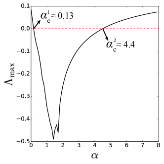
Figure 35: Master stability function for x-coupled Rössler attractors on a network structure.

Stability region where $\Lambda$ is negative is bounded between $\alpha_{c}^{1}\approx 0.13$ and $\alpha_{c}^{2}\approx 4.4$. So, if the network is a complete graph then $\lambda_{2}=\cdots=\lambda_{N}=N$, so the network synchronization when

$$\frac{\alpha_{c}^{2}}{N}>\alpha>\frac{\alpha_{c}^{1}}{N}$$

6.2 Synchronization conditions and Synchronization Loss

In Sec .5.1, we discussed the synchronizability of network types when there is only one critical threshold in other words $\alpha_{c}^{2}\rightarrow\infty$. This case is true when H is a positive matrix. In the general case, there are two finite critical couplings Eq. 68 and the master stability function has a finite stability region between these critical points (as discussed in the above section). Now we discuss this synchronization scenario for various network types. To quantify the synchronizability, we will use the network properties given in Table. 1.

2$k$-regular graphs – Diameter driven synchronization loss.

When $k<<N$, the mean geodesic distance (shortest path length) between nodes are increasing very fast as $N$ increasing. Hence, while the diameter of the network is increasing $d=2N/k$, speed of information exchange between the nodes is decreasing drastically. In this case, the complete synchronization is not stable and it is visible from the Laplacian spectrum of the graph. For $N\to\infty$ and $k<<N$, the extremal eigenvalues given in Table 1 can be extended to Taylor expansion and major role playing part can be rewritten as

$$\lambda_{2}=\frac{4\pi^{2}(k+\frac{1}{2})^{3}}{3N^{2}}\mbox{ and }\lambda_{N}=2k\frac{N}{N-1}$$

The ratio between the largest $\lambda_{N}$ and second smallest eigenvalue $\lambda_{2}$ of the Laplacian is not growing in the same scale,

$$\frac{\lambda_{N}}{\lambda_{2}}\approx N^{2}/k^{2}$$

and the condition in Eq. (68) is never satisfied.

ER graphs – Optimal Synchronization.

In this case, the extremal eigenvalues $\lambda_{2}$ and $\lambda_{n}$ of the Laplacian matrix increase in the same scale. The diameter of the network increases very slowly $d\approx\log N$ when the network size $N$ increases Table 1. Therefore the synchronization is stable for any scale of size.

BA networks – Heterogeneity driven synchronization loss.

When the network is too heterogeneous the complete synchronization is unstable, this is because the extremal eigenvalues $\lambda_{2}$ and $\lambda_{N}$ grow in different scales and the condition in Eq. (68) is never met. For instance, consider a BA network. Then, the eigenvalues satisfy

$$\lambda_{2}\approx m\mbox{ and }\lambda_{N}\approx mN^{1/2}$$

where $m$ is the mean degree. Hence, the eigenration becomes

$$\frac{\lambda_{N}}{\lambda_{2}}\approx N^{1/2}$$

this should be compared to the stability interval given by the master stability function. Lets consider the example in the above section with the Rössler Eq. (70). The master stability function gives (as seen in Figure 35) an stability interval $\alpha_{c}^{2}/\alpha_{c}^{1}\approx 34$. The stability conditions Eq. (68) reads as

$$N^{1/2}<34$$

So, when the BA network is large enough it is not possible to synchronize the system. In particular the critical system size to be able to synchronization a network of Rössler as in Eq. (70) is, therefore,

$$N\approx 10^{3}.$$

6.2.1 Extensions

There are a few extensions of the model. Here we discuss a few directions.

Directed Networks.

The major problem considering directed networks is that they may not be diagonalizable. So, the decoupling of transversal modes by projection is a nontrvial steps. There are a few ways to overcome this. The first, using Jordan decomposition of the Laplacian. The other possibility is to perturb the Laplacian to make the eigenvalues simples. This must be done in such a way that the perturbation does not spoil the stability. In both cases, the stability condition remain unchanged. Only the transients may be longer.

When the network is nondiagonalizable, small perturbations in the network may lead to large perturbations in the eigenvalues (the eigenvalues in this case are not differentiable functions of the perturbations) [77]. Moreover, structural improvements in the network may lead to desynchronization [81].

Nonidentical Nodes

Here we consider $f(x)\mapsto f(x)+r_{i}(x,t)$, where $r_{i}$ is either a perturbation of the vector field or a signal playing the role of noise. When $r_{i}$ is very small synchronization will persist [14]. For general networks, Bollt and co-workers [120] extended the master stability function approach when $r_{i}$ is a perturbation of the vector field. Pereira and co-workers [93] study the effect of general perturbations $\|r_{i}\|\leq\delta$ and the role that the network structure plays in suppressing the fluctuations. In the case where H is positive definite and the network is undirected, they showed that the synchronization error

$$E=\frac{1}{n(n-1)}\sum_{ij}\|x_{i}-x_{j}\|$$

behaves as

$$E\leq K\frac{\delta}{\alpha\lambda_{2}-\alpha_{c}}$$

For example, if the oscillators where uncoupled and $r_{i}$ independent noise then the Central Limit theorem would yield $E=O(N^{-1/2}).$ For complete networks, the interaction and synchronization yields $E=O(N^{-1})$ which is a large improvement over the naive application of the Central Limit theorem. In certain sense, this shows that interacting maybe better then isolation.

Nonidentical Coupling Functions

In many applications the coupling function are not identical and has fluctuating components [115]. Consider an undirected networks of identical oscillators and coupling function

$$H_{ij}(x_{i}-x_{j},t)=H(x_{i}-x_{j})+P_{ij}(x_{i}-x_{j},t)$$

where $\|P_{ij}(x_{i}-x_{j},t)\|\leq\eta$. In this case, the network structure will play a major on the size of perturbation $\eta$. If the network is random and the degree distribution homogeneous, then even for large perturbations $\delta$ synchronization is stable. If the network is heterogeneous degrees such as Barabasi-Albert then typically $\delta_{c}=O(N^{-\beta})$ is the critical perturbation size. If $\delta>\delta_{c}$ synchronization becomes unstable, solely because of the interaction between network structure and perturbations in the coupling function.

Cluster Synchronization

According to similarities in coupled systems, such as symmetries in network topology or identical dynamics in a diverse population or equally time-delayed nodes in differently distributed feedbacks, the partial or cluster synchronization can emerge. In order to enlighten the reason of these cluster synchronization cases, many techniques are developed and experimental observations are analyzed[133, 17, 111, 27, 36, 126].

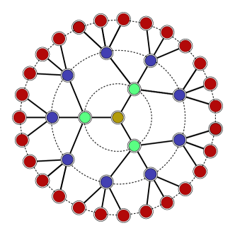
Figure 36: Bethe lattice graph: an example of symmetries in network structure. Nodes in the same level of the Bethe graph are exactly symmetric to each other. Therefore same color nodes constitute a cluster.

The symmetries are easy to detect for some network geometries for instance Bethe lattice is a regular graph which grows from a root (parent) node by $m$-nodes for $\ell$-levels, an example of Bethe lattice given in Fig. 36 for $m=3$ and $\ell=3$. The nodes in the same level of the Bethe graph, they all symmetric to each other. In Fig. 36, the levels of the graph are given in the same color and the cluster synchronization occurs for each level.

Recently, Pecora et al. put forward that all the symmetries in network structures are not visible directly. They developed a computational group theory based method to reveal these hidden symmetries and predicted possible synchronization patterns [88, 112].

Time Delay Coupling

Simultaneous coupling is not always possible for real world applications in other words some time delays can occur in the interaction process. Therefore it is important to investigate synchronizability and stability of coupled time-delayed systems. The necessary conditions for time delayed synchronization is analytically shown by Pyragas [98]. The finding of time-delay synchronization is used as an application for the anticipating synchronization (see Section 3.4).

Appendix A List of frequently used notions and abbreviations

Table of notions

$|\cdot|$	absolute value
$\|\cdot\|$	norm
$\delta_{ij}$	Kroneker delta
$G$	graph
L	Laplacian matrix
A	adjacency matrix
I	identity matrix
H	coupling function
1	vector whose every components is 1
$\alpha$	coupling strength
$\alpha_{c}$	critical coupling strength for synchronization
f	isolated dynamics (vector field)
$\Lambda$	Maximum Lyapunov exponent
$\lambda_{2}$	spectral gap: the second minimum eigenvalue of Laplacian matrix
$D\textbf{\em f}$	Jacobian matrix of f
$\phi$	phase
$t$	time
$a,b$ and $c$	parameters of Rössler system
$\sigma,\rho$ and $\beta$	parameters of Lorenz system
$m$ and $n$	dimensions of vector fields
$i$ and $j$	natural numbers
$N$	system size of networks
$M$	total number of links
$k_{i}$	degree of $i$-th node
$d$	diameter of a network

Table of abbreviations

CS	complete synchronization
PS	phase synchronization
GS	generalized synchronization
AS	anticipating synchronization
ER	Erdös - Renyi network
SF	Scale-free network
SW	Small world network
BA	Barabasi - Albert network

Appendix B Lyapunov exponent

Sensitive dependence on initial conditions is one of the main characteristics of chaotic systems. The main idea is that nearby orbits diverge at an exponential rate. This rate is called Lyapunov exponents. In this Appendix, we provide the basic notions on the theory of Lyapunov exponents.

If we have a nonlinear equation we can study the properties of a given solution s by linearizing the dynamics around the orbit, as we have done in Sec 2.2. This procedure leads to a linear nonautonomous equation

$$v^{\prime}=A\left(t\right)v$$

where $A$ is continuous and bounded matrix function. The goal is to study the behaviour of solutions. Typically solving the equation explicitly is impossible. So the theory of Lyapunov exponents plays a major role.

Let $v:\mathbb{R}\rightarrow\mathbb{R}^{n}$ be a solution $v^{\prime}=A\left(t\right)v$ and $T(t,s)$ is the fundamental matrix. The Lyapunov exponent of the solution is defined as

$$\lambda\left(v\right)=\overline{\lim_{t\rightarrow\infty}}\frac{1}{t}\ln\left\|T(t,s)v(s)\right\|$$

We also define $\lambda\left(0\right)=-\infty$. The largest Lyapunov exponents is our main object of study and is given by

$$\Lambda=\overline{\lim_{t\rightarrow\infty}}\frac{1}{t}\ln\left\|\Pi\left(t,s\right)\right\|$$

it determines the behaviour of solutions asymptotically because for any solution of the equation we have

$$\left\|v\left(t\right)\right\|<C_{\varepsilon}e^{\left(\Lambda+\varepsilon\right)t}$$

If $\Lambda<0$, the trivial solution $v\left(t\right)=0$ is asymptotically stable. Lyapunov exponents generalizes stability criteria for autonomous (given by eigenvalues) and periodic equations (given by Floquet exponents).

Lemma B.1.

Let $A\in Mat\left(n\right)$ and $v$ be an eigenvector of $Av=\beta v$. Then $\lambda\left(v\right)=\beta$.

If all $\lambda\left(v\right)<0$, we have $\max_{v}\left\{\lambda\left(v\right)\right\}=\Lambda<0$, and the trivial solution is asymptotically stable. The Lyapunov exponent also generalizes the Floquet exponents.

Lemma B.2.

Let $A\left(t\right)$ be a periodic matrix by the Floquet representation we have $T(t,s)=P(t,s)e^{(t-s)Q(s)}$. Let $v$ be an eigenvector of $Q\left(s\right)$, then $\lambda\left(v\right)$ is an eigenvalue of $Q(s)$.

Hence, Lyapunov exponents are the eigenvalues of the monodromy matrix $Q$. Although, for the synchronization analysis we care about the maximal Lyapunov exponents, it is important to know that there are at most $n$ distinct Lyapunov exponents because the set $X=\left\{v\left(t\right)|\lambda\left(v\right)\leq\alpha\right\}$ is a vector space.

Appendix C Lyapunov Function

One of the main techniques to tackle stability of nonlinear system is the Lyapunov function method. The method by Lyapunov allows us to obtain the stability without finding the trajectories by studying properties of the Lyapunov function. We consider a dynamical system is modelled by a differential equation

$$\dot{\textbf{\em x}}=\frac{d\textbf{\em x}}{dt}=\textbf{\em f}(\textbf{\em x})$$ (71)

We will study notions relative to connected nonempty subsets $\Omega$ of $\mathbb{R}^{m}$. A function $V:\mathbb{R}^{m}\rightarrow\mathbb{R}$ is said to be positive definite with respect to the set $B$ if $V(\textbf{\em x})>0$ for all $\textbf{\em x}\in\mathbb{R}^{q}\backslash\Omega$. It is radially unbounded if

$$\lim_{\|\textbf{\em x}\|\rightarrow\infty}V(\textbf{\em x})=\infty.$$

Note that this condition guarantees that all level sets of $V$ are bounded. This fact plays a central role in the analysis. We also define $V^{\prime}:\mathbb{R}^{m}\rightarrow\mathbb{R}$ as

$$V^{\prime}(\textbf{\em x})=\nabla V(\textbf{\em x})\cdot\textbf{\em f}(\textbf{\em x}).$$

where $\cdot$ denotes the Euclidean inner product. This definition agrees with the time derivative along the trajectories. That is, if $\textbf{\em x}(t)$ is a solution of Eq. (71), then by the chain rule we have

$$\frac{dV(\textbf{\em x}(t))}{dt}=V^{\prime}(\textbf{\em x}(t)).$$

Notice that applying the chain rule we obtain

$$V^{\prime}(\textbf{\em x}(t))=\nabla V(\textbf{\em x}(t))\cdot\textbf{\em f}(\textbf{\em x}(t))$$

This has a nice geometric interpretation. Since $\nabla V(\textbf{\em x}(t))$ is perpendicular to the level set of $V$ if $V^{\prime}(\textbf{\em x}(t))<0$ it means that the vector field is point inwards the level set and trajectories will enter the level set and never leave it. Repeating the argument we obtain stability as the following statement shows

Theorem 4 (Lyapunov).

Let $V:\mathbb{R}^{m}\rightarrow\mathbb{R}$ be radially unbounded and positive definite with respect to the set $\Omega\subset D$. Assume that

$$V^{\prime}(\textbf{\em x})<0\mbox{ for all }\textbf{\em x}\in\mathbb{R}^{m}\backslash\Omega$$

Then all trajectories of Eq. (71) eventually enter the set $\Omega$, in other words, the system is dissipative.

There are also converse Lyapunov theorems [65]. Typically if the system is dissipative (and have nice properties) then there exists a Lyapunov function. Although the above theorem is very useful, since we don’t need knowledge of the trajectories, the drawback is the function $V$ itself. There is no recipe to obtain a function $V$ fulfilling all these properties. One could always try to guess the function, or go for a general form such as choosing a quadratic function $V$. We assume that the Lyapunov function is given.

Appendix D Chaos in Lorenz system

In order to understand the behaviour of a continuous system, we can use the concept of a Poincaré section – a transversal surface to the flow. This method was developed by Henri Poincaré in 1890s. The crossing points are a set of discrete numbers and this number sequence is called Poincaré map. We can study the structure of the crossings of the trajectory to the surface. This reduces the dimension of the system by $1$. The structure of crossing points between the plane and the trajectory determines the behaviour of the system. For example, if the trajectory cross the section always at same $k$-coordinate points and repeat these points in the same order then the system is periodic so-called period-$k$.

The maxima of $z$-component of the Lorenz system, which is Poincaré section of velocities, graphically show the chaotic regime clearly. The governing equation of the Poincaré map ($\{z_{n}\}$) can be plotted as ${z_{n}}$ vs ${z}_{n+1}$ (Fig. 37 (a)) which resembles the tent map function (Fig. 37 (b)). The tent map is given by

$$f(x_{n})=x_{n+1}=\left\{\begin{array}[]{ll}2x_{n}&0\leq x_{n}\leq 1/2\\ 2-2x_{n}&1/2<x_{n}\leq 1.\end{array}\right.$$

Lyapunov exponent of the tent map

$$\Lambda=\lim_{t\rightarrow\infty}\frac{1}{t}\ln\|Df(x)\|$$ (72)

where $Df$ is the Jacobian of $f$ and $\|Df(x)\|=2\mbox{ for all }x\neq 1/2$ since the function is not differentiable at $x=1/2$. Therefore the Lyapunov exponent is $\Lambda=\ln 2$ and according to the positive Lyapunov exponent, the behaviour of the system is chaotic.

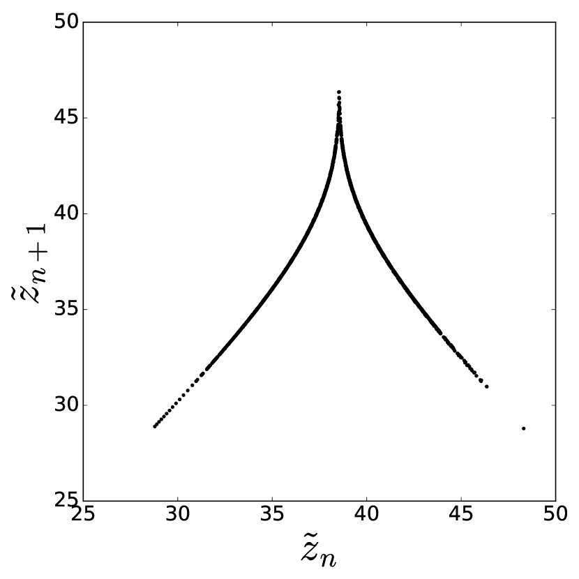
(a) Lorenz system

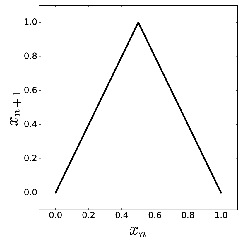
(b) Tent map

Figure 37: Similarity between Poincaré map of Lorenz system and the tent map.

The definition of chaos given by Devaney is the the following let $X$ be a metric space and a continuous map $f:X\to X$ is chaotic if

1. $f$ is transitive (indecomposability); that is any non-empty intervals $U,V\subset X$ there exist a natural number $k$ such that $f^{k}(U)\cap V$. The transitivity condition ensures the irreducibility of $X$, means that $X$ is an open invariant set and cannot split into two open invariant sets.

2. the periodic trajectories of $f$ are dense in X (an element of regularity); that is every point in the attractor of $f$ will return back to neighbourhood of the initial point. In other words, any trajectory initiating from an interval $I\subset X$, will be back in $I$ in sufficiently long but finite time. Therefore the subset $I$ contains infinitely many periodic points.

3. $f$ has sensitive dependence on initial conditions (unpredictability); that is if there is an infinitesimal distance $\delta_{0}$ between any two point $x,y\in X$ and there exists a nonnegative number $k$ such that after $n$ iterations the distance between $f^{n}(x)$ and $f^{n}(y)$ is larger than $\delta_{n}>\delta_{0}$. These nearly started orbits diverge from each other at a rate $\Lambda$ (see Appendix B).

   More details can be found in the reference [46].

Appendix E Mathematical Structure of Generalized Synchronization

For completeness, we include this brief discussion of the mathematical structure of GS and it may be skipped without harm to the remaining sections. Again lets consider the $\psi:\mathbb{R}^{m}\rightarrow\mathbb{R}^{n}$ and the manifold

$$M=\{(x,y)\in\mathbb{R}^{n}\times\mathbb{R}^{m}:y=\psi(x)\}\subset\mathbb{R}^{n+m}.$$

GS corresponds to the case where $M$ is normally attracting. Lets review the notion of normally attracting invariant manifold (NAIM). $M$ is normally attracting if it is invariant under the flow $\Phi$ (of the full system) and the dynamics in the directions normal to $M$ is contracting stronger than in direction tangential to $M$. That is,

1. (Invariance) $\Phi^{t}(M)=M$ for all $t$,

2. (Normal Contraction) There is a continuous splitting of the tangent space

   $$\forall x\in M:\,\,\,\,T_{x}\mathbb{R}^{n+m}=T_{x}M\oplus E_{x}^{s}$$

   which is left invariant by $D\Phi^{t}$. Moreover, there is $\eta>0$ such that

   $$\forall t\geq 0,x\in M,v\in E_{x}^{s}:\,\,\,\|D\Phi^{t}(x)v\|\leq Ce^{-\eta}\|v\|$$

3. (Contraction in the normal directions dominate the tangential) There exist $r>1$, $\lambda>0$ and $C>0$ such that

   $$\forall t\geq 0,x\in M:\,\,\,\|D\Phi^{t}(x)\left|{}_{E_{x}^{s}}\right.\|\leq Ce^{-\lambda t}\|D\Phi^{-t}(x)\left|{}_{T_{x}M}\right.\|^{-r}$$

If $M$ is a NAIM for the system $F$. Then there exist locally invariant stable manifolds $W_{loc}^{s}(M)$ such that $W_{loc}^{s}(M)$ is tangent to $TM\oplus E_{s}$ at $M$ and $W_{s}(M)\in C^{r}$. Moreover, $W_{loc}^{s}(M)$ consists of all points near $M$ whose forward orbit converges to $M$ at rate $e^{-\eta t}$. For each $y\in W_{s}(M)$ shadows a point $x\in M$ such that $y\in W^{s}_{loc}(x)$ and

$$\|\Phi^{t}(y)-\Phi^{t}(x)\|\leq Ce^{-\eta t}\|y-x\|$$ (73)

Since the orbits of points $x_{0},x_{1}\in M$ cannot approach each other that fast, we can characterize points $y\in W_{loc}^{s}(x)$ precisely as those that satisfy Eq. (73). Lets consider consider the straithening of the manifold. That is, we introduce new coordinates

$$u=y-\psi(x)$$

in this coordinates the manifold corresponds to the $x$ axis and $u$ are the normal directions to $M$. Lets take two points $u_{1},u_{0}\in W_{loc}^{s}(x)$ then

$$u_{i}=y_{i}-\psi(x)\Rightarrow u_{1}-u_{0}=y_{1}-y_{0}$$

Hence, if

$$\|y_{1}-y_{0}\|\leq Ke^{-\eta t}$$

and $\eta$ is larger than the smallest Lyapunov exponents of the driver in modulus the manifold $M$ will be normally attracting, according to condition (3). In fact, $\psi$ will be differentiable. Another important fact to the mention is that NAIM persist under small perturbations. For us this means that once we obtain GS small perturbations such as increasing the coupling strength will be destroy GS [33, 34]. If the condition is not satisfied then $\psi$ won’t be a NAIM. However, it may still happen that when $r=0$ and $M$ is attracting. In this case, $\psi$ is only continuous. This is called strong and weak generalized synchronization [51].

Back to our Diffusively driven oscillator. In Sec. LABEL:XX we showed the contraction rate between two nearby trajectories is

$$\eta=\alpha\lambda_{min}-\|Dg\|$$

On the other hand, the smallest Lyapunov exponent of the driver is at most $-\|Df\|$, hence the condition for normal attraction is

$$\eta>\|Df\|\Rightarrow\alpha>\frac{\|Df\|+\|Dg\|}{\lambda_{min}}$$

This gives the bound for $M$ to be NAIM.

References

- Abarbanel et al. [1996] Abarbanel, H. D. I., Rulkov, N. F., and Sushchik, M. M. (1996). Generalized synchronization of chaos: The auxiliary system approach. Physical Review E, 53(5):4528–4535.
- Afraimovich et al. [1986] Afraimovich, V. S., Verichev, N. N., and Rabinovich, M. I. (1986). Stochastic synchronization of oscillation in dissipative systems. Izvestiya Vysshikh Uchebnykh Zavedenii, Radiofizika, 29(9):795–803.
- Albert and Barabási [2002] Albert, R. and Barabási, A.-L. (2002). Statistical mechanics of complex networks. Reviews of Modern Physics, 74(January):48–94.
- Albert et al. [2000] Albert, R., Jeong, H., and Barabási, A.-L. (2000). Error and attack tolerance of complex networks. Nature, 406(July):378–381.
- Arenas et al. [2008] Arenas, A., Díaz-Guilera, A., Kurths, J., Moreno, Y., and Zhou, C. (2008). Synchronization in complex networks. Physics Reports, 469(3):93–153.
- Ashwin et al. [1994] Ashwin, P., Buescu, J., and Stewart, I. (1994). Bubbling of attractors and synchronisation of chaotic oscillators. Physics Letters A, 193(2):126–139.
- Ashwin et al. [1998] Ashwin, P., Terry, J. R., Thornburg, K. S., and Roy, R. (1998). Blowout bifurcation in a system of coupled chaotic lasers. Physical Review E, 58(6):7186–7189.
- Balanov et al. [2009] Balanov, A., Janson, N., Postnov, D., and Sosnovtseva, O. (2009). Synchronization: From Simple to Complex. Springer-Verlag Berlin Heidelberg.
- Baptista et al. [2006] Baptista, M. S., Pereira, T., and Kurths, J. (2006). Upper bounds in phase synchronous weak coherent chaotic attractors. Physica D, 216(2):260–268.
- Baptista et al. [2005] Baptista, M. S., Pereira, T., Sartorelli, J. C., Caldas, I. L., and Kurths, J. (2005). Non-transitive maps in phase synchronization. Physica D, 212(3-4):216–232.
- Baptista et al. [2003] Baptista, M. S., Silva, T. P., Sartorelli, J. C., Caldas, I. L., and Rosa, E. (2003). Phase synchronization in the perturbed Chua circuit. Physical Review E, 67:056212.
- Barabási and Albert [1999] Barabási, A.-L. and Albert, R. (1999). Emergence of Scaling in Random Networks. Science, 286(October):509–512.
- Barahona and Pecora [2002] Barahona, M. and Pecora, L. M. (2002). Synchronization in Small-World Systems. Physical Review Letters, 89(5):054101 (1–4).
- Belykh et al. [2003] Belykh, I., Belykh, V., Nevidin, K., and Hasler, M. (2003). Persistent clusters in lattices of coupled nonidentical chaotic systems. Chaos, 13(1):165–178.
- Belykh et al. [2005] Belykh, I., De Lange, E., and Hasler, M. (2005). Synchronization of bursting neurons: What matters in the network topology. Physical Review Letters, 94(18):1–4.
- Belykh et al. [2016] Belykh, I., Jeter, R., and Belykh, V. (2016). Foot force models of crowd dynamics on a wobbly bridge. arXiv:1610.05366v1, pages 1–15.
- Belykh et al. [2008] Belykh, V. N., Osipov, G. V., Petrov, V. S., Suykens, J. A. K., and Vandewalle, J. (2008). Cluster synchronization in oscillatory networks. Chaos, 18(3):037106 (1–6).
- Bode et al. [2010] Bode, N. W. F., Faria, J. J., Franks, D. W., Krause, J., and Wood, a. J. (2010). How perceived threat increases synchronization in collectively moving animal groups. Proc. R. Soc. B, 277(1697):3065–70.
- Bollobás [1998] Bollobás, B. (1998). Modern Graph Theory. Springer-Verlag New York.
- Carroll et al. [1996] Carroll, T. L., Heagy, J., and Pecora, L. M. (1996). Transforming signals with chaotic synchronization. Physical Review E, 54(5):4676–4680.
- Carroll and Pecora [1998] Carroll, T. L. and Pecora, L. M. (1998). Synchronizing Hyperchaotic Volume-Preserving Maps and Circuits. IEEE Trans. Circuits Syst., I: Fund. Theory and App, 45(6):656–659.
- Chen et al. [2003] Chen, J. Y., Wong, K. W., Cheng, L. M., and Shuai, J. W. (2003). A secure communication scheme based on the phase synchronization of chaotic systems. Chaos, 13(2):508–514.
- Chen et al. [2001] Chen, J. Y., Wong, K. W., Zheng, H. Y., and Shuai, J. W. (2001). Phase signal coupling induced n:m phase synchronization in drive-response oscillators. Physical Review E, 63(3):036214 (1–6).
- Chung and Lu [2006] Chung, F. and Lu, L. (2006). Complex Graphs and Networks. American Mathematical Society.
- Cuomo and Oppenheim [1993a] Cuomo, K. M. and Oppenheim, A. V. (1993a). Chaotic signals and systems for communications. IEEE, 4:137–140.
- Cuomo and Oppenheim [1993b] Cuomo, K. M. and Oppenheim, A. V. (1993b). Circuit Implementation of Synchronized Chaos with Applications to Communications. Physical Review Letters, 71(1):65–68.
- Dahms et al. [2012] Dahms, T., Lehnert, J., and Schöll, E. (2012). Cluster and group synchronization in delay-coupled networks. Physical Review E, 86(1):016202 (1–10).
- Dedieu et al. [1993] Dedieu, H., Kennedy, M. P., and Hasler, M. (1993). Chaos shift keying: modulation and demodulation of a chaotic carrier using self-synchronizing Chua’s circuits. IEEE Trans. Circuits Syst., II: Analog Digital Signal Processing, 40(10):634–642.
- Dedieu and Ogorzalek [1997] Dedieu, H. and Ogorzalek, M. J. (1997). Identifiability and identification of chaotic systems based on adaptive synchronization. IEEE Trans. Circuits Syst., I: Fund. Theory and App, 44(10):948–962.
- Earn et al. [2000] Earn, D. J. D., Levin, S. A., and Rohani, P. (2000). Coherence and Conservation. Science, 290(November):1360–1364.
- Earn et al. [1998] Earn, D. J. D., Rohani, P., and Grenfell, B. T. (1998). Persistence, chaos and synchrony in ecology and epidemiology. Proc R. Soc. Lond. B, 265(1390):7–10.
- Eckhardt et al. [2007] Eckhardt, B., Ott, E., Strogatz, S. H., Abrams, D. M., and McRobie, A. (2007). Modeling walker synchronization on the millennium bridge. Physical Review E, 75(2):021110 (1–10).
- Eldering [2013] Eldering, J. (2013). Normally Hyperbolic Invariant Manifolds. Atlantis Press.
- Fenichel [1972] Fenichel, N. (1972). Persistence and Smoothness of Invariant Manifolds for Flows.
- Fiedler [1973] Fiedler, M. (1973). Algebraic connectivity of graphs. Czechoslovak Mathematical Journal, 23(2):298–305.
- Fu et al. [2013] Fu, C., Deng, Z., Huang, L., and Wang, X. (2013). Topological control of synchronous patterns in systems of networked chaotic oscillators. Physical Review E, 87(3):032909 (1–7).
- Fujisaka and Yamada [1983] Fujisaka, H. and Yamada, T. (1983). Stability Theory of Synchronized Motion in Coupled-Oscillator Systems. Progress of Theoretical Physics, 69(1):32–47.
- Garcia Dominguez et al. [2005] Garcia Dominguez, L., Wennberg, R. A., Gaetz, W., Cheyne, D., Snead, O. C., and Perez Velazquez, J. L. (2005). Enhanced synchrony in epileptiform activity? Local versus distant phase synchronization in generalized seizures. The Journal of Neuroscience, 25(35):8077–8084.
- Gleick [2011] Gleick, J. (2011). Chaos: Making a New Science (Enhanced Edition). Open Road Media.
- Gregoriou et al. [2009] Gregoriou, G. G., Gotts, S. J., Zhou, H., and Desimone, R. (2009). High-Frequency, Long-Range Coupling Between Prefrontal and Visual Cortex During Attention. Science, 324(5931):1207–1210.
- Grenfell et al. [2001] Grenfell, B. T., Bjørnstad, O. N., and Kappey, J. (2001). Travelling waves and spatial hierarchies in measles epidemics. Nature, 414:716–723.
- Hammond et al. [2007] Hammond, C., Bergman, H., and Brown, P. (2007). Pathological synchronization in Parkinson’s disease: networks, models and treatments. Trends in Neurosciences, 30(7):357–364.
- He and Vaidya [1992] He, R. and Vaidya, P. G. (1992). Analysis and synthesis of synchronous periodic and chaotic systems. Physical Review A, 46(12):7387–7392.
- Heagy et al. [1995] Heagy, J. F., Pecora, L. M., and Carroll, T. L. (1995). Short Wavelength Bifurcations and Size Instabilities in Coupled Oscillator Systems. Physical Review Letters, 74(21):4185–4188.
- Hirosawa et al. [2013] Hirosawa, K., Kittaka, S., Oishi, Y., Kannari, F., and Yanagisawa, T. (2013). Phase locking in a Nd:YVO4 waveguide laser array using Talbot cavity. Optics Express, 21(21):24952–24961.
- Hirsch et al. [2004] Hirsch, M., Smale, S., and Devaney, R. (2004). Differential Equations, Dynamical Systems, and an Introduction to Chaos. Number v. 60 in Differential equations, dynamical systems, and an introduction to chaos. Academic Press.
- Hodgkin and Huxley [1952] Hodgkin, A. L. and Huxley, A. F. (1952). A quantitative description of membrane current and its application to conduction and excitation in nerve. J Physiol., 117(4):500–544.
- Hramov and Koronovskii [2004] Hramov, A. E. and Koronovskii, A. A. (2004). An approach to chaotic synchronization. Chaos, 14(3):603–610.
- Hramov and Koronovskii [2005] Hramov, A. E. and Koronovskii, A. A. (2005). Generalized synchronization: A modified system approach. Physical Review E, 71(6):067201 (1–4).
- Huang et al. [2009] Huang, L., Chen, Q., Lai, Y. C., and Pecora, L. M. (2009). Generic behavior of master-stability functions in coupled nonlinear dynamical systems. Physical Review E, 80:1–11.
- Hunt et al. [1997] Hunt, B. R., Ott, E., and Yorke, J. A. (1997). Differentiable generalized synchronization of chaos. Physical Review E, 55(4):4029–4034.
- Jeffreys and Jeffreys [1988] Jeffreys, H. and Jeffreys, B. (1988). Mean-Value Theorems. Cambridge University Press, 3rd edition edition.
- Josić and Mar [2001] Josić, K. and Mar, D. J. (2001). Phase synchronization of chaotic systems with small phase diffusion. Physical Review E, 64(5):056234 (1–10).
- Kapitaniak et al. [2014] Kapitaniak, M., Czolczynski, K., Perlikowski, P., Stefanski, A., and Kapitaniak, T. (2014). Synchronous states of slowly rotating pendula. Physics Reports, 541(1):1–44.
- Katok and Hasselblatt [1997] Katok, A. and Hasselblatt, B. (1997). Introduction to the Modern Theory of Dynamical Systems. Encyclopedia of Mathematics and its Applications. Cambridge University Press.
- Kocarev et al. [1992] Kocarev, L., Halle, K. S., Eckert, K., Chua, L. O., and Parlitz, U. (1992). Experimental Demonstration of Secure Communications Via Chaotic Synchronization. International Journal of Bifurcation and Chaos, 02(03):709–713.
- Kocarev and Parlitz [1995] Kocarev, L. and Parlitz, U. (1995). General Approach for Chaotic Synchronization with Applications to Communication. Physical Review Letters, 74(25):5028–5031.
- Kocarev and Parlitz [1996] Kocarev, L. and Parlitz, U. (1996). Generalized Synchronization, Predictability, and Equivalence of Unidirectionally Coupled Dynamical Systems. Physical Review Letters, 76(11):1816–1819.
- Kocarev et al. [1996a] Kocarev, L., Parlitz, U., and Stojanovski, T. (1996a). An application of synchronized chaotic dynamic arrays. Physics Letters A, 217(4-5):280–284.
- Kocarev et al. [1996b] Kocarev, L., Parlitz, U., Stojanovski, T., and Panovski, L. (1996b). Generalized synchronization of chaos. 1996 IEEE International Symposium on Circuits and Systems. Circuits and Systems Connecting the World. ISCAS 96, 3:116–119.
- Kowalski et al. [1990] Kowalski, J. M., Albert, G. L., and Gross, G. W. (1990). Asymptotically synchronous chaotic orbits in systems of excitable elements. Physical Review A, 42(10):6260–6263.
- Kuramoto [1975] Kuramoto, Y. (1975). Self-Entrainment of a Population of Coupled Non-Linear Oscillators. Lecture Notes in Physics, 39(International Symposium on Mathematical Problems in Theoretical Physics):420–423.
- Lorenz [1963] Lorenz, E. N. (1963). Deterministic Nonperiodic Flow. Journal of the Atmospheric Sciences, 20(2):130–141.
- Lotrič and Stefanovska [2000] Lotrič, M. B. and Stefanovska, A. (2000). Synchronization and modulation in the human cardiorespiratory system. Physica A, 283(3):451–461.
- Lyapunov [1992] Lyapunov, A. M. (1992). Stability of motion: general problem. International Journal of Control, 55(3):767–772.
- Masoller [2001] Masoller, C. (2001). Anticipation in the synchronization of chaotic semiconductor lasers with optical feedback. Physical Review Letters, 86(13):2782–2785.
- Mohar [1991a] Mohar, B. (1991a). Eigenvalues, diameter, and mean distance in graphs. Graphs and Combinatorics, 7(1):53–64.
- Mohar [1991b] Mohar, B. (1991b). The Laplacian Spectrum of Graphs. Graph Theory, Combinatorics, and Applications, Vol. 2, 2:871–898.
- Mohar [1997] Mohar, B. (1997). Some applications of Laplace eigenvalues of graphs, pages 225–275. Springer Netherlands, Dordrecht.
- Motter et al. [2013] Motter, A. E., Myers, S. a., Anghel, M., and Nishikawa, T. (2013). Spontaneous synchrony in power-grid networks. Nature Physics, 9(3):191–197.
- Motter et al. [2005a] Motter, A. E., Zhou, C., and Kurths, J. (2005a). Network synchronization, diffusion, and the paradox of heterogeneity. Physical Review E, 71(1):016116 (1–9).
- Motter et al. [2005b] Motter, A. E., Zhou, C. S., and Kurths, J. (2005b). Enhancing complex-network synchronization. Europhysics Letters, 69(3):334–340.
- Murphy et al. [2010] Murphy, T. E., Cohen, A. B., Ravoori, B., Schmitt, K. R. B., Setty, A. V., Sorrentino, F., Williams, C. R. S., Ott, E., and Roy, R. (2010). Complex dynamics and synchronization of delayed-feedback nonlinear oscillators. Phil. Trans. R. Soc. A, 368(1911):343–366.
- Néda et al. [2000] Néda, Z., Ravasz, E., Brechet, Y., Vicsek, T., and Barabási, A.-L. (2000). The sound of many hands clapping. Nature, 403(6772):849–850.
- Newman [2003] Newman, M. E. J. (2003). The Structure and Function of Complex Networks. SIAM Review, 45(2):167–256.
- Newman [2010] Newman, M. E. J. (2010). Networks: An introduction. Oxford University Press.
- Nishikawa and Motter [2010] Nishikawa, T. and Motter, A. E. (2010). Network synchronization landscape reveals compensatory structures, quantization, and the positive effect of negative interactions. Proceedings of the National Academy of Sciences of the United States of America, 107(23):10342–7.
- Nishikawa et al. [2003] Nishikawa, T., Motter, A. E., Lai, Y.-C., and Hoppensteadt, F. C. (2003). Heterogeneity in Oscillator Networks: Are Smaller Worlds Easier to Synchronize? Physical Review Letters, 91(1):014101.
- Oliva and Strogatz [2001] Oliva, R. A. and Strogatz, S. H. (2001). Dynamics of a Large Array of Globally Coupled Lasers With Distributed Frequencies. International Journal of Bifurcation and Chaos, 11(09):2359–2374.
- Oppenheim et al. [1992] Oppenheim, A. V., Wornell, G. W., Isabelle, S. H., and Cuomo, K. M. (1992). Signal processing in the context of chaotic signals. International Conference on Acoustics, Speech, and Signal Processing, 1992, 4:117–120.
- Pade and Pereira [2015] Pade, J. P. and Pereira, T. (2015). Improving Network Structure can lead to Functional Failures. Scientific reports, 5:9968.
- Parlitz [1996] Parlitz, U. (1996). Estimating Model Parameters from Time Series by Autosynchronization. Physical Review Letters, 76(8):1232–1235.
- Parlitz et al. [1992] Parlitz, U., Chua, L. O., Kocarev, L., Halle, K. S., and Shang, A. (1992). Transmission of Digital Signals By Chaotic Synchronization. International Journal of Bifurcation and Chaos, 02(04):973–977.
- Parlitz et al. [1996] Parlitz, U., Junge, L., and Kocarev, L. (1996). Synchronization-based parameter estimation from time series. Physical Review E, 54(6):6253–6259.
- Pecora and Carroll [1990] Pecora, L. M. and Carroll, T. L. (1990). Synchronization in chaotic systems. Physical Review Letters, 64(8):821–824.
- Pecora and Carroll [1991] Pecora, L. M. and Carroll, T. L. (1991). Driving systems with chaotic signals. Physical Review A, 44(4):2374–2383.
- Pecora and Carroll [1998] Pecora, L. M. and Carroll, T. L. (1998). Master Stability Functions for Synchronized Coupled Systems. Physical Review Letters, 80(10):2109–2112.
- Pecora et al. [2014] Pecora, L. M., Sorrentino, F., Hagerstrom, A. M., Murphy, T. E., and Roy, R. (2014). Cluster synchronization and isolated desynchronization in complex networks with symmetries. Nature communications, 5(May):4079.
- Peng et al. [1996] Peng, J. H., Ding, E. J., Ding, M., and Yang, W. (1996). Synchronizing Hyperchaos with a Scalar Transmitted Signal. Physical Review Letters, 76(6):904–907.
- Pereira [2010] Pereira, T. (2010). Hub synchronization in scale-free networks. Physical Review E, 82(3):036201 (1–4).
- Pereira et al. [2007] Pereira, T., Baptista, M. S., and Kurths, J. (2007). Phase and average period of chaotic oscillators. Physics Letters A, 362(2-3):159–165.
- Pereira et al. [2014] Pereira, T., Eldering, J., Rasmussen, M., and Veneziani, A. (2014). Towards a general theory for coupling functions allowing persistent synchronization. Nonlinearity, 27:501–525.
- Pereira et al. [2013] Pereira, T., Eroglu, D., Bagci, G. B., Tirnakli, U., and Jensen, H. J. (2013). Connectivity-driven coherence in complex networks. Physical Review Letters, 110(23):234103 (1–5).
- Perez and Cerdeira [1995] Perez, G. and Cerdeira, H. A. (1995). Extracting messages masked by chaos. Physical Review Letters, 74(11):1970–1973.
- Pikovsky et al. [2001] Pikovsky, A., Rosenblum, M., and Kurths, J. (2001). Synchronization: A universal concept in nonlinear sciences. Cambridge University Press, Cambridge.
- Pikovsky et al. [1997] Pikovsky, A. S., Rosenblum, M. G., Osipov, G. V., and Kurths, J. (1997). Phase synchronization of chaotic oscillators by external driving. Physica D, 104(3-4):219–238.
- Powell [1964] Powell, M. J. D. (1964). An efficient method for finding the minimum of a function of several variables without calculating derivatives. The Computer Journal, 7(2):155–162.
- Pyragas [1998] Pyragas, K. (1998). Synchronization of coupled time-delay systems: Analytical estimations. Physical Review E, 58(3):3067–3071.
- Ren et al. [2013] Ren, H.-P., Baptista, M. S., and Grebogi, C. (2013). Wireless communication with chaos. Physical Review Letters, 110(18):184101 (1–5).
- Riordan and Selby [2000] Riordan, O. and Selby, A. (2000). The maximum degree of a random graph. Comb. Probab. Comput., 9(6):549–572.
- Rodrigues et al. [2016] Rodrigues, F. A., Peron, T. K. D., Ji, P., and Kurths, J. (2016). The Kuramoto model in complex networks. Physics Reports, 610:1–98.
- Rosenblum et al. [1996] Rosenblum, M. G., Pikovsky, A. S., and Kurths, J. (1996). Phase synchronization of chaotic oscillators. Physical Review Letters, 76(3):1804.
- Rosenblum et al. [1997] Rosenblum, M. G., Pikovsky, A. S., and Kurths, J. (1997). From Phase to Lag Synchronization in Coupled Chaotic Oscillators. Physical Review Letters, 78(22):4193–4196.
- Rulkov et al. [1995] Rulkov, N. F., Sushchik, M. M., Tsimring, L. S., and Abarbanel, H. D. I. (1995). Generalized synchronization of chaos in directionally coupled chaotic systems. Physical Review E, 51(2):980–994.
- Sanders et al. [2007] Sanders, J. A., Verhulst, F., and Murdock, J. (2007). Averaging Methods in Nonlinear Dynamical Systems, volume 59. Springer-Verlag New York, second edition.
- Schäfer et al. [1998] Schäfer, C., Rosenblum, M. G., Kurths, J., and Abel, H. H. (1998). Heartbeat synchronized with ventilation. Nature, 392(6673):239–240.
- Schultz et al. [2016] Schultz, P., Peron, T., Eroglu, D., Stemler, T., Ramírez Ávila, G. M., Rodrigues, F. A., and Kurths, J. (2016). Tweaking synchronization by connectivity modifications. Physical Review E, 93(6):062211.
- Shiogai et al. [2010] Shiogai, Y., Stefanovska, A., and McClintock, P. V. E. (2010). Nonlinear dynamics of cardiovascular ageing. Physics Reports, 488(2-3):51–110.
- Short [1994] Short, K. M. (1994). Step toward unmasking secure communications. International Journal of Bifurcation and Chaos, 4(4):959—-977.
- Singer [1999] Singer, W. (1999). Neuronal Synchrony: A Versatile Code Review for the Definition of Relations. Neuron, 24:49–65.
- Sorrentino and Ott [2007] Sorrentino, F. and Ott, E. (2007). Network synchronization of groups. Physical Review E, 76(5):056114 (1–10).
- Sorrentino and Pecora [2016] Sorrentino, F. and Pecora, L. M. (2016). Approximate cluster synchronization in networks with symmetries and parameter mismatches. Chaos, 26(9):094823.
- Sparrow [1982] Sparrow, C. (1982). The Lorenz Equations: Bifurcations, Chaos, and Strange Attractors. Springer-Verlag New York.
- Stankovski et al. [2014] Stankovski, T., McClintock, P. V. E., and Stefanovska, A. (2014). Coupling functions enable secure communications. Physical Review X, 4(1):011026 (1–9).
- Stankovski et al. [2015] Stankovski, T., Ticcinelli, V., McClintock, P. V. E., and Stefanovska, A. (2015). Coupling functions in networks of oscillators. New Journal of Physics, 17.
- Stefanovska et al. [2001] Stefanovska, A., Lotric, M. B., Strle, S., and Haken, H. (2001). The cardiovascular system as coupled oscillators? Physiological measurement, 22(3):535–550.
- Strogatz [2003] Strogatz, S. H. (2003). Sync: The Emerging Science of Spontaneous Order. Hyperion.
- Strogatz et al. [2005] Strogatz, S. H., Abrams, D. M., McRobie, A., Eckhardt, B., and Ott, E. (2005). Crowd synchrony on the Millennium Bridge. Nature, 438(November):43–44.
- Sugawara et al. [1994] Sugawara, T., Tachikawa, M., Tsukamoto, T., and Shimizu, T. (1994). Observation of synchronization in laser chaos. Physical Review Letters, 72(22):3502–3505.
- Sun et al. [2009] Sun, J., Bollt, E. M., and Nishikawa, T. (2009). Master Stability Functions for Coupled Near-Identical Dynamical Systems. EPL (Europhysics Letters), 60011:11.
- Tass et al. [1998] Tass, P., Rosenblum, M. G., Weule, J., Kurths, J., Pikovsky, A., Volkmann, J., Schnitzler, A., and Freund, H.-J. (1998). Detection of n:m Phase Locking from Noisy Data: Application to Magnetoencephalography. Physical Review Letters, 81(15):3291–3294.
- Tönjes [2010] Tönjes, R. (2010). Synchronization transition in the Kuramoto model with colored noise. Physical Review E, 81:055201.
- Tönjes and Blasius [2009] Tönjes, R. and Blasius, B. (2009). Perturbation analysis of the Kuramoto phase-diffusion equation subject to quenched frequency disorder. Physical Review E, 79:016112.
- Viana [2000] Viana, M. (2000). What’s new on lorenz strange attractors? Math. Intelligencer, 22(3):6–19.
- Wiesenfeld et al. [1996] Wiesenfeld, K., Colet, P., and Strogatz, S. H. (1996). Synchronization Transitions in a Disordered Josephson Series Array. Physical Review Letters, 76(3):404–407.
- Williams et al. [2013] Williams, C. R. S., Murphy, T. E., Roy, R., Sorrentino, F., Dahms, T., and Schöll, E. (2013). Experimental observations of group synchrony in a system of chaotic optoelectronic oscillators. Physical Review Letters, 110(6):064104 (1–5).
- Winfree [1967] Winfree, A. T. (1967). Biological rhythms and the behavior of populations of coupled oscillators. Journal of Theoretical Biology, 16(1):15–42.
- Winful and Rahman [1990] Winful, H. G. and Rahman, L. (1990). Synchronized chaos and spatiotemporal chaos in arrays of coupled lasers. Physical Review Letters, 65(13):1575–1578.
- Wu [2003] Wu, C. W. (2003). Perturbation of coupling matrices and its effect on the synchronizability in arrays of coupled chaotic systems. Physics Letters A, 319(5-6):495–503.
- Yamada and Fujisaka [1983] Yamada, T. and Fujisaka, H. (1983). Stability Theory of Synchronized Motion in Coupled-Oscillator Systems. II. Progress of Theoretical Physics, 70(5):1240–1248.
- Yamada and Fujisaka [1984] Yamada, T. and Fujisaka, H. (1984). Stability Theory of Synchronized Motion in Coupled-Oscillator Systems. III. Progress of Theoretical Physics, 72(5):885–894.
- Yu and Parlitz [2008] Yu, D. and Parlitz, U. (2008). Estimating parameters by autosynchronization with dynamics restrictions. Physical Review E, 77(6):066221 (1–7).
- Zhou and Kurths [2006] Zhou, C. and Kurths, J. (2006). Hierarchical synchronization in complex networks with heterogeneous degrees. Chaos, 16(1):015104 (1–10).
- Zhou et al. [2006] Zhou, C., Motter, A. E., and Kurths, J. (2006). Universality in the Synchronization of Weighted Random Networks. Physical Review Letters, 96(3):034101 (1–4).