MSE estimates for multitaper spectral estimation and off-grid compressive sensing

Luís Daniel Abreu labreu@kfs.oeaw.ac.at  and  José Luis Romero jlromero@kfs.oeaw.ac.at Acoustics Research Institute, Austrian Academy of Science, Wohllebengasse 12-14 A-1040, Vienna, Austria
Abstract.

We obtain estimates for the Mean Squared Error (MSE) for the multitaper spectral estimator and certain compressive acquisition methods for multi-band signals. We confirm a fact discovered by Thomson [Spectrum estimation and harmonic analysis, Proc. IEEE, 1982]: assuming bandwidth $W$ and $N$ time domain observations, the average of the square of the first $K=\left\lfloor 2NW\right\rfloor$ Slepian functions approaches, as $K$ grows, an ideal band-pass kernel for the interval $\left[-W,W\right]$. We provide an analytic proof of this fact and measure the corresponding rate of convergence in the $L^{1}$ norm. This validates a heuristic approximation used to control the MSE of the multitaper estimator. The estimates have also consequences for the method of compressive acquisition of multi-band signals introduced by Davenport and Wakin, giving MSE approximation bounds for the dictionary formed by modulation of the critical number of prolates.

L. D. A. was supported by the Austrian Science Fund (FWF) START-project FLAME (”Frames and Linear Operators for Acoustical Modeling and Parameter Estimation”) Y 551-N13. J. L. R. gratefully acknowledges support from the Austrian Science Fund (FWF): P 29462 - N35 and from a Marie Curie fellowship, within the 7th. European Community Framework program, under grant PIIF-GA-2012-327063. The authors also acknowledge support from the WWTF grant INSIGHT (MA16-053).

1. Introduction

The discrete prolate spheroidal sequences (DPSS), introduced by Slepian in [34], play a fundamental role both in Thomson’s multitaper method for spectral estimation of stationary processes [37], and in the method proposed by Davenport and Wakin for compressive acquisition of multi-band analog signals in the presence of off-grid frequencies [9]. (See also [16, 11, 3, 18].)

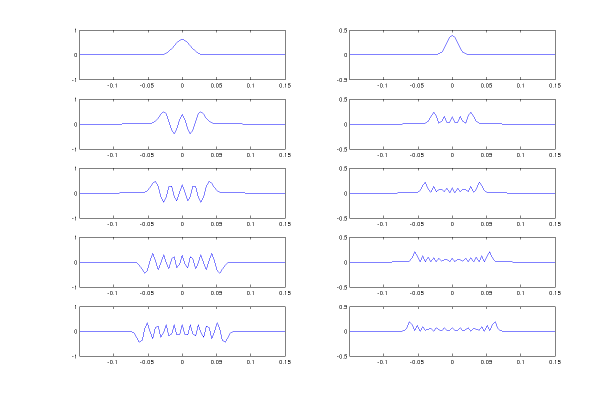
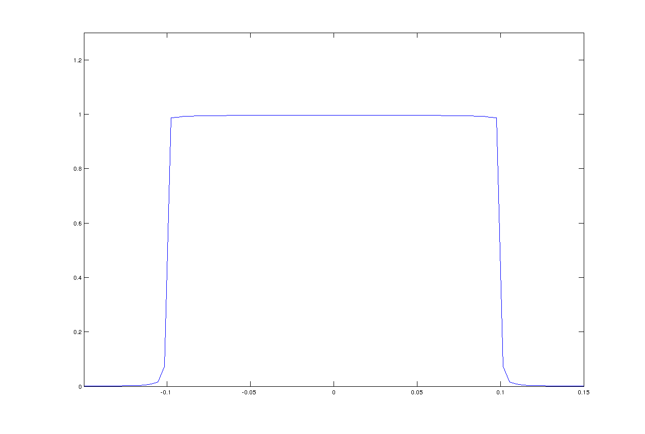
In this article we provide Mean Squared Error (MSE) estimates for both methods based on the following observation: while the description of each individual discrete Slepian function can be very subtle, the aggregated behavior of the critical number of solutions displays a simple profile, that can be quantified (see Figures 1 and 2).

Our bounds for the expectation of Thomson’s estimator validate some heuristics from [37] and elaborate on more qualitative work [7, 22]. Similar performance bounds were until now only available for modified versions of Thomson’s method, that replace the Slepian sequences with other tapers that have analytic expressions [29].

2. Thomson’s multitaper method

Let $I=\left[-1/2,1/2\right]$. Any stationary, real, ergodic, zero-mean, Gaussian stochastic process has a Cramér spectral representation

$$x(t)=\int_{I}e^{2\pi i\xi t}dZ(\xi)\text{,}$$

and the spectrum $S(\xi)$, defined as

$$S(\xi)d\xi=\mathbb{E}\{\left|dZ(\xi)\right|^{2}\}\text{,}$$

and often called the power spectral density of the process, yields the periodic components of $x(t)$. The goal of spectral estimation is to solve the highly underdetermined problem of estimating $S(\xi)$  from a sample of $N$ contiguous observations $x(0),...,x(N-1)$. Embryonic approaches to the problem [36, 30] used the so called periodogram:

(2.1) $$\widehat{S}(\xi)=\frac{1}{N}\left|\sum_{t=0}^{N-1}x(t)e^{-2\pi i\xi t}\right|^{2},$$

whose analysis has influenced harmonic analysts since Norbert Wiener (see [5]). The periodogram can also be weighted with a data window $\left\{D_{t}\right\}_{t=0}^{N-1}$, usually called a taper, giving the estimator:

(2.2) $$\widehat{S}_{D}(\xi)=\left|\sum_{t=0}^{N-1}x(t)D_{t}e^{-2\pi i\xi t}\right|^{2}\text{.}$$

The choice of the taper $\left\{D_{t}\right\}_{t=0}^{N-1}$ can have a significant effect on the resulting spectrum estimate $\widehat{S}_{D}$. This is apparent by observing that its expectation is the convolution of the true (nonobservable) spectrum $S(\xi)$ with the spectral window $\left|\mathcal{F}D(\xi)\right|^{2}=\left|\sum_{t=0}^{N-1}D_{t}e^{-2\pi i\xi t}\right|^{2}$, i.e.,

(2.3) $$\mathbb{E}\left\{\widehat{S}_{D}(\xi)\right\}=S(\xi)\ast\left|\mathcal{\ F}D(\xi)\right|^{2}.$$

Thus, the bias of the tapered estimator, which is the difference $S(\xi)-\mathbb{E}\{\widehat{S}_{D}(\xi)\}$, is determined by the smoothing effect of $\left\{D_{t}\right\}_{t=0}^{N-1}$ over the true spectrum. Ideally, the function $\mathcal{F}D(\xi)$ should be concentrated on the interval $[-\tfrac{1}{2N},\tfrac{1}{2N}]$, but the uncertainty principle of Fourier analysis precludes such perfect concentration (see e.g. [16]).

In [37], Thomson used the DPSS basis to construct an algorithm that averages several tapered estimates, whence the name multitaper. Thomson’s multitaper method has been used in a variety of scientific applications including climate analysis (see, for instance [6], or [12] for a local spherical approach), statistical signal analysis [26], and it was used to better understand the relation between atmospheric $CO_{2}$ and climate change (see [38, Section 1]).

Today, Thomson’s multitaper method remains an effective spectral estimation method. It has recently found remarkable applications in electroencephalography [10] and it is the preferred spectral sensing procedure [13] for the rapidly emerging field of cognitive radio [14] [16, Chapter 3]. In the next paragraph we provide an outline of the method.

Thomson’s method starts by selecting a target frequency smoothing band $[-W,W]$ with $1/2N<W<1/2$, thus accepting a reduction in spectral resolution by a factor of about $2NW$. The first step consists of obtaining a number $K=\left\lfloor 2NW\right\rfloor$ (the smallest integer not greater than $2NW$) of estimates of the form (2.2) by setting, for every $k\in\{0,...,K-1\}$, $D_{t}=v_{t}^{(k)}(N,W)$, where the discrete prolate spheroidal sequences $v_{t}^{(k)}(N,W)$ are defined as the solutions of the Toeplitz matrix eigenvalue equation

(2.4) $$\sum_{n=0}^{N-1}\frac{\sin 2\pi W\left(t-n\right)}{\pi\left(t-n\right)}v_{n}^{(k)}(N,W)=\lambda_{k}(N,W)v_{t}^{(k)}(N,W),$$

and normalized by $||v^{(k)}||_{2}=1$. The resulting tapered periodogram is then denoted by $\widehat{S}_{k}(\xi)$. The second step consists of averaging. One uses the estimator

(2.5) $$\widehat{S}_{(K)}(\xi)=\frac{1}{K}\sum_{k=0}^{K-1}\widehat{S}_{k}(\xi),$$

which achieves a reduced variance (see [37] for an asymptotic analysis of slowly varying spectra and [40, 22] for non-asymptotic expressions).

To inspect the performance of the estimator $\widehat{S}_{(K)}(\xi)$ on the spectral domain, let us consider the discrete prolate spheroidal functions, also known as Slepians. They are the discrete Fourier transforms of the sequences $v_{t}^{(k)}(N,W)$, denoted by $U_{k}(N,W;\xi)$, and satisfy the integral equation

(2.6) $$\int_{-W}^{W}\mathbf{D}_{N}(\xi-\xi^{\prime})U_{k}(N,W;\xi^{\prime})d\xi^{\prime}=\lambda_{k}(N,W)U_{k}(N,W;\xi)\text{,}$$

where

(2.7) $$\mathbf{D}_{N}(x)=\frac{\sin N\pi x}{\sin\pi x}$$

is the Dirichlet kernel. Observe that, according to (2.3), $\mathbb{E}\{\widehat{S}_{k}(\xi)\}$ is a smoothing average of the unobservable spectrum by the kernel $\left|U_{k}(N,W;\xi)\right|^{2}$. Recall that the bias of each individual estimate in (2.5) is given by

(2.8) $$Bias\left(\widehat{S}_{k}(\xi)\right)=\mathbb{E}\{\widehat{S}_{k}(\xi)\}-S(\xi)=S(\xi)\ast\left|U_{k}(N,W;\xi)\right|^{2}-S(\xi).$$

The optimal concentration of the first prolate function on the interval $[-W,W]$ leads to a low bias when $k=0$. But since the amount of energy of $U_{k}(N,W;\xi)$ inside $[-W,W]$ decreases with $k$ (because the energy is given by the eigenvalues in (2.6) and they decrease from $1$ to just above 00 as $k$ crosses the critical value $K$), the bias may increase for large values of $k$. Let us inspect the averaged estimator. Its expectation is

(2.9) $$\mathbb{E}\{\widehat{S}_{(K)}(\xi)\}=\frac{1}{K}\sum_{k=0}^{K-1}\mathbb{E}\{\widehat{S}_{k}(\xi)\}=S(\xi)\ast\frac{1}{K}\rho_{K}(N,W;\xi)\text{, }$$

where

(2.10) $$\frac{1}{K}\rho_{K}(N,W;\xi)=\frac{1}{K}\sum_{k=0}^{K-1}\left|U_{k}(N,W;\xi)\right|^{2}.$$

To explain the bias performance of the averaged estimator, Thomson [37, Section 4] observed that the spectral window (2.10) is very similar to a flat function localized on $[-W,W]$ (see Figures 1 and 2). This is an intriguing mathematical phenomenon. Heuristically, it requires the functions in the sequence $\{\left|U_{k}(N,W,\cdot)\right|^{2}:k=0,\ldots,K-1\}$ to be organized inside the interval $[-W,W]$ in a very particular way: each function tends to fill in the empty energy spots left by the sum of the previous ones - a behavior reminiscent of the Pythagorean relation for pure frequencies: $\sin^{2}(t)+\cos^{2}(t)=1$. More precisely, claiming that the spectral window in Thomson’s method approximates an ideal band-pass kernel means that the two functions

(2.11) $$\frac{1}{K}\rho_{K}(N,W,.)\text{ \ \ \ and \ \ \ \ }\frac{1}{2W}\mathbf{1}_{[-W,W]}\text{,}$$

approach each other as $K$ increases. This is indeed true and we provide an analytic bound for the $L^{1}$-distance between the functions in (2.11).

Theorem 2.1 (Spectral leakage estimate).

Let $N\geq 2$ be an integer, $W\in(-1/2,1/2)$ and set $K:=\left\lfloor 2NW\right\rfloor$. Then

(2.12) $$\left\|\frac{1}{K}\rho_{K}(N,W,\cdot)-\frac{1}{2W}\mathbf{1}_{[-W,W]}\right\|_{L^{1}(I)}\lesssim\frac{\log N}{K}.$$
Refer to caption
Figure 1. Slepians $U_{k}$ and their squares $\left|U_{k}\right|^{2}$, for $N=256$ and $W=0.1$ and $k=1,5,9,19$.
Refer to caption
Figure 2. Thomson’s spectral window, with $N=256$ and $W=0.1$.

The estimate (2.12) is precisely what we need in order to quantify Thomson’s asymptotic analysis of the bias of the multitaper estimator [37, pg.. 1062] and validate the bias-variance trade-off. Indeed, the $L^{1}$ deviation estimate allows one to control the effect of replacing the spectral window by an ideal kernel in (2.9). This is explained in detail in Section 4.

As an alternative to (2.5), Thomson also considered a modified method, where all Slepian sequences are used as tapers - instead of just the first $K$ - but the corresponding tapered periodograms are weighted with the eigenvalues. In this case, a similar analysis applies and the spectral window is:

(2.13) $\displaystyle\tilde{\rho}_{K}(N,W,\xi):=\sum_{k=0}^{N-1}\lambda_{k}(N,W)\left|U_{k}(N,W;\xi)\right|^{2}.$

We provide similar bounds for the modified method.

Theorem 2.2.

Let $N\geq 2$ be an integer and $W\in(-1/2,1/2)$. Then

(2.14) $$\left\|\frac{1}{K}\tilde{\rho}_{K}(N,W,\cdot)-\frac{1}{2W}\mathbf{1}_{[-W,W]}\right\|_{L^{1}(I)}\lesssim\frac{\log N}{K}.$$

3. Analysis of Thomson’s spectral window

Let $I:=[-1/2,1/2]$ and let us denote the exponentials by $e_{\omega}(x):=e^{2\pi ix\omega}$. We will always let $N\geq 2$ be an integer and $W\in(-1/2,1/2)$. For two non-negative functions $f,g$, the notation $f\lesssim g$ means that there exists a constant $C>0$ such that $f\leq Cg$. (The constant $C$, of course, does not depend on the parameters $N,W$.)

We normalize the Slepian functions by $\int_{I}\left|U_{k}(N,W;\xi)\right|^{2}\,d\xi=1$. We will need a description of the profile of the eigenvalues in (2.4). The following lemma will be key in most of the estimates.

Lemma 3.1.

For $N\geq 2$, $W\in(-1/2,1/2)$ and $K:=\left\lfloor 2NW\right\rfloor$:

(3.1) $$\left|1-\frac{1}{K}\sum_{k=0}^{K-1}\lambda_{k}(N,W)\right|\lesssim\frac{\log N}{K}.$$

We postpone the proof of Lemma 3.1 to Section 7. The quantity on the left-hand side of (3.1) has been studied in [22] to qualitatively analyze the performance of Thomson’s method. Lemma 3.1 refines the analysis of [22], giving a concrete growth estimate. (See also the remarks after Theorem 5 in [22].)

3.1. Proof of Theorem 2.1

We first estimate the narrow band error. Note that

$$\rho_{K}(N,W;\xi)=\sum_{k=0}^{K-1}\left|U_{k}(N,W;\xi)\right|^{2}\leq\sum_{k=0}^{N-1}\left|U_{k}(N,W;\xi)\right|^{2}=D_{N}(0)=N\text{.}$$

Consequently, $\tfrac{1}{K}\rho_{K}(N,W;\xi)\leq\tfrac{N}{K}$ and, using (7.2), we can estimate:

$\displaystyle\int_{-W}^{W}\left|\frac{1}{K}\rho_{K}(N,W;\xi)-\frac{1}{2W}\mathbf{1}_{[-W,W]}(\xi)\right|\,d\xi$
$\displaystyle\qquad\leq\int_{-W}^{W}\left|\left(\frac{1}{2W}-\frac{N}{K}\right)\mathbf{1}_{[-W,W]}(\xi)\right|\,d\xi+\int_{-W}^{W}\left|\frac{1}{K}\rho_{K}(N,W;\xi)-\frac{N}{K}\mathbf{1}_{[-W,W]}(\xi)\right|\,d\xi$
$\displaystyle\qquad=2W\left(\frac{N}{K}-\frac{1}{2W}\right)+\frac{2NW}{K}-\frac{1}{K}\sum_{k=0}^{K-1}\int_{-W}^{W}\left|U_{k}(N,W;\xi)\right|^{2}\,d\xi$
$\displaystyle\qquad\leq\frac{2}{K}+1-\frac{1}{K}\sum_{k=0}^{K-1}\lambda_{k}\lesssim\frac{\log N}{K},$

thanks to Lemma 3.1. Now we estimate the broad brand leakage:

$\displaystyle\int_{I\setminus[-W,W]}\left|\frac{1}{K}\rho_{K}(N,W;\xi)-\frac{1}{2W}\mathbf{1}_{[-W,W]}(\xi)\right|\,d\xi=\int_{I\setminus[-W,W]}\frac{1}{K}\rho_{K}(N,W;\xi)\,d\xi$
$\displaystyle\qquad=\frac{1}{K}\sum_{k=0}^{K-1}(1-\lambda_{k})=1-\frac{1}{K}\sum_{k=0}^{K-1}\lambda_{k},$

so the conclusion follows invoking again Lemma 3.1.

3.2. Proof of Theorem 2.2

See Section 7.4.

4. MSE bounds for Thomson’s multitaper

In [37, Section IV], Thomson estimated $Bias(\widehat{S}_{(K)})$ by using the approximation $\frac{1}{K}\rho_{K}(N,W,\cdot)\approx\frac{1}{2W}\mathbf{1}_{[-W,W]}$. Using Theorem 2.1 we inspect that approximation:

$$\left|Bias(\widehat{S}_{(K)}(\xi))\right|\leq\left|\left|S*\frac{1}{K}\rho_{K}(N,W,\cdot)-S*\frac{1}{2W}\mathbf{1}_{[-W,W]}\right|\right|_{\infty}+\left|\left|S-S*\frac{1}{2W}\mathbf{1}_{[-W,W]}\right|\right|_{\infty}$$

and, if $S$ is a bounded function, then Theorem 2.1 implies that

$$\left|\left|S*\frac{1}{K}\rho_{K}(N,W,\cdot)-S*\frac{1}{2W}\mathbf{1}_{[-W,W]}\right|\right|_{\infty}\lesssim\left|\left|S\right|\right|_{\infty}\frac{\log N}{K}.$$

(Similar considerations apply to the modified estimator where tapered periodograms are weighted by the corresponding eigenvalue; in that case we invoke Theorem 2.2.) The remaining term $\left|\left|S-S*\frac{1}{2W}\mathbf{1}_{[-W,W]}\right|\right|_{\infty}$ can be bounded by assuming that $S$ is smooth. For example, if, as in Thomson’s work, $S$ is assumed to $C^{2}$ (as a periodic function), then $\left|\left|S-S*\frac{1}{2W}\mathbf{1}_{[-W,W]}\right|\right|_{\infty}\lesssim W^{2}$, leading to the bias estimate:

(4.1) $$\mathrm{Bias}(\widehat{S}_{(K)}(\xi))\lesssim W^{2}+\frac{\log N}{K}.$$

On the other hand, for a slowly varying spectrum $S$, Thomson [37] argues that

(4.2) $$\mathrm{Var}\left(\widehat{S}_{(K)}(\xi)\right)\lesssim\frac{1}{K}\text{, }$$

(see, [40], [22] or [16, Section 3.1.2] for precise expressions for the variance; in particular [22, Theorem 2] for the bound in (4.2), valid when $S\in L^{\infty}$.) Given a number of available observations, the estimates in (4.1) and (4.2) show how much bias can be expected, in order to bring the variance down by a factor of $1/K$. This leads to a concrete estimate for the mean squared error

$\displaystyle\mathrm{MSE}(\widehat{S}_{(K)}(\xi))$ $\displaystyle=\mathbb{E}(S(\xi)-\widehat{S}_{(K)}(\xi))^{2}$
$\displaystyle=\mathrm{Bias}(\widehat{S}_{(K)}(\xi))^{2}+\mathrm{Var}(\widehat{S}_{(K)}(\xi))$
$\displaystyle\lesssim W^{4}+\frac{\log^{2}N}{K^{2}}+\frac{1}{K},$

that can be used to decide on the value of the bandwidth resolution parameter $W$.

Thus, in the slowly varying regime, the error due to spectral leakage is largely dominated by the variance and therefore, in agreement with Thomson’s analysis, the mean squared error is $\lesssim W^{4}+\frac{1}{K}\asymp\left(\frac{K}{N}\right)^{4}+\frac{1}{K}$. We note that the value of $K$ that minimizes this expression satisfies $K\asymp N^{4/5}$ and gives

$\displaystyle\mathrm{MSE}(\widehat{S}_{(K)}(\xi))\lesssim N^{-4/5}.$

A similar relation holds for the so-called minimum bias sinusoidal tapers [29]. (Recall that $K$ and $W$ are related by $K=\lfloor 2NW\rfloor$; choosing a certain value for $K$ amounts to choosing a corresponding value for $W$.)

5. Compressive acquisition of multi-band signals

An important step in signal processing is to provide finite-dimensional models that adequately capture analog phenomena. This problem is delicate and naive discretizations can lead to poor reconstruction. A concrete instance of the modeling problem occurs in the study of the compressive acquisition of multi-band signals: their naive representation suffers from the so-called DFT leakage. (See [11] and [3] for the modeling problem in compressive sensing, including multi-scale settings.)

Let $\Delta\subseteq\mathbb{R}$ be an interval with $\left|\Delta\right|\leq 1$ that is decomposed as union of disjointly translated copies of a smaller interval $[-W,W]$:

$$\Delta=\bigcup_{j=0}^{M-1}[-W,W]+\{2Wj\}.$$

We consider a so-called multi-band signal $x(t)$ whose Fourier transform is supported on the union of $L\ll M$ translated copies of $[-W,W]$, say

(5.1) $$\Delta_{\ast}=\bigcup_{n=0}^{L-1}[-W,W]+\{2Wj_{n}\},$$

with $j_{n}\in\{0,\ldots,M-1\}$. In order to acquire such a signal, the problem is to efficiently represent the corresponding sampled vector

$$\mathbf{x}=(x(0),\ldots,x(N-1)).$$

Davenport and Wakin [9] proposed using the dictionary of modulated Slepian sequences

(5.2) $$\mathcal{D}:=\{e^{-2\pi i(2Wj)(\boldsymbol{\cdot})}v^{(k)}:k=0,\ldots K-1,j=0,\ldots,M-1\},$$

where $K\approx 2NW$ is a parameter and $v^{(k)}=v^{(k)}(N,W)$ are the discrete prolate spheroidal sequences. The sampled vector $\mathbf{x}$ is expected to have an approximately $LK$-sparse representation in $\mathcal{D}$. More precisely, the sampled vector $\mathbf{x}$ associated with a signal $x$ with Fourier transform supported on the set $\Delta_{\ast}$ from (5.1) is expected to be approximately captured by the sub-dictionary

(5.3) $$\mathcal{D}_{\ast}:=\{e^{-2\pi i(2Wj_{n})(\boldsymbol{\cdot})}v^{(k)}:k=0,\ldots K-1,n=0,\ldots,L-1\}.$$

For the critical value $K=\left\lfloor 2NW\right\rfloor$ we obtain the following average case estimate.

Theorem 5.1.

Let $x(t)=\tfrac{1}{L}\sum_{n=0}^{L-1}x_{n}(t)$ be the average of independent, continuous-time, zero-mean, Gaussian stationary random processes $x_{n}(t)$ with corresponding power spectra $S_{x_{n}}:=\frac{1}{2W}\mathbf{1}_{[-W,W]+\{2Wj_{n}\}}$. Let $\mathcal{D}_{*}$ be the dictionary in (5.3) with $K=\left\lfloor 2NW\right\rfloor$. For $N\geq 2$, let $\mathbf{x}=(x(0),\ldots,x(N-1))$ be the vector of finite samples of $x$, and $P_{\mathcal{D}_{*}}\mathbf{x}$ its projection onto the linear span of $\mathcal{D}_{*}$. Then

$\displaystyle\frac{\mathbb{E}\left\{||\mathbf{x}-P_{\mathcal{D}_{*}}\mathbf{x}||^{2}\right\}}{\mathbb{E}\left\{||\mathbf{x}||^{2}\right\}}\lesssim\frac{L\log N}{K}.$
Proof.

Theorem 4.4 in [9] gives ${\mathbb{E}\left\{||\mathbf{x}||^{2}\right\}}=N$ and

$${\mathbb{E}\left\{||\mathbf{x}-P_{\mathcal{D}_{\ast}}\mathbf{x}||^{2}\right\}}\leq\frac{L}{2W}\sum_{k=K}^{N-1}\lambda_{k}(N,W).$$

Since $2NW=\sum_{k=0}^{N-1}\lambda_{k}(N,W)$ and $K=\left\lfloor 2NW\right\rfloor$, we can use Lemma 3.1 to conclude that

$\displaystyle\frac{\mathbb{E}\left\{||\mathbf{x}-P_{\mathcal{D}_{\ast}}\mathbf{x}||^{2}\right\}}{\mathbb{E}\left\{||\mathbf{x}||^{2}\right\}}$ $\displaystyle\leq$ $\displaystyle\frac{L}{K}\sum_{k=K}^{N-1}\lambda_{k}(N,W)$
$\displaystyle\leq$ $\displaystyle L\left(1-\frac{1}{K}\sum_{k=0}^{K-1}\lambda_{k}(N,W)+\frac{1}{K}\right)$
$\displaystyle\lesssim$ $\displaystyle\frac{L\log N}{K}.$

Remark 5.2.

Approximation estimates such as the one in Theorem 5.1 quantify the rate at which a finite dimensional model captures an analog phenomenon and are therefore instrumental to the quantification of the so-called stable sampling rate in compressive sensing [3].

Remark 5.3.

Theorem 5.1 applies to the critical number of Slepian sequences. Better approximation rates are possible by increasing the number of dictionary elements, see [9, Section 5] and [42, Corollary 3.12].

6. Conclusions and outlook

We provided a quantitative description of the spectral window of Thomson’s multitaper method, leading to MSE bounds. We also quantified in the mean-squared sense the effectiveness of the dictionary of modulated Slepian functions to capture analog multi-band signals.

An accumulation phenomenon similar to the one in Theorem 2.1 has been investigated in [2] and numerically illustrated in [4, 8]. We therefore expect our approach to be applicable to other estimators including the one based on spherical Slepians [31, 8], and those for non-stationary spectra [23, 15, 4, 24, 27, 39, 25].

Eigenvalue estimates for the spectral concentration problem are available in the context of Hankel bandlimited functions [1]. We expect these to be useful for problems involving $2D$ functions whose spectrum lies on a disk, a setting relevant in cryo-electron microscopy, where estimation of noise stochastics is an important consideration when applying PCA [41].

Dictionaries similar to the one in (5.2) also appear in [17], in the context of prolate-spheroidal functions on the line. As shown in [17], corresponding frame properties are related to a variant of Thomson’s spectral window. For this reason, it would be interesting to obtain a version of Theorem 2.1 for the $L^{\infty}$-norm.

7. Technical lemmas

7.1. Trigonometric polynomials and Toeplitz operators

Our proof uses tools from the Landau-Pollack-Slepian theory [32, 35, 19, 20, 21]. For notational convenience, we use a temporal normalization that is slightly different from the one in Section 2 (this has no impact in the announced estimates). We consider the space of trigonometric polynomials

$$\mathcal{P}_{N}=Span\left\{e_{\frac{-N+1}{2}+j}:0\leq j\leq N-1\right\}\subseteq L^{2}\left(I\right)\text{.}$$

This is a Hilbert space with a reproducing kernel given by the translated Dirichlet kernel, $\mathbf{D}_{N}(x-y)$,  $x,y\in I$ $N\geq 2$, where $\mathbf{D}_{N}$ is given by (2.7). Note that $\int_{I}\left|\mathbf{D}_{N}\right|^{2}=N$.

For $W\in(-1/2,1/2)$ the Toeplitz operator $H_{W}^{N}$ is

(7.1) $$H_{W}^{N}f:=P_{{\mathcal{P}_{N}}}\left((P_{\mathcal{P}_{N}}f)\cdot 1_{[-W,W]}\right),\qquad f\in L^{2}(I),$$

where $P_{{\mathcal{P}_{N}}}$ is the orthogonal projection onto $\mathcal{P}_{N}$. When $f\in\mathcal{P}_{N}$, $H_{W}^{N}f$ is simply the projection of $f\cdot 1_{[-W,W]}$ into $\mathcal{P}_{N}$. The Slepian functions $\{U_{k}(N,W):k=0,\ldots,N-1\}$ are the eigenfunctions of $H_{W}^{N}$ with corresponding eigenvalues $\lambda_{k}=\lambda_{k}(N,W)$:

(7.2) $$\int_{-W}^{W}\left|U_{k}(N,W;\xi)\right|^{2}\,d\xi=\lambda_{k},$$

ordered non-increasingly. We normalize the Slepian functions by $\int_{I}\left|U_{k}(N,W;\xi)\right|^{2}\,d\xi=1$.

7.2. Integral kernels

The Toeplitz operator $H_{W}^{N}$ from (7.1) can be explicitly described by the formula

$$H_{W}^{N}f(x)=\int_{I}f(y)K_{W}^{N}(x,y)dy\text{,}$$

where the kernel $K_{W}^{N}(x,y)$ is

(7.3) $$K_{W}^{N}(x,y)=\int_{[-W,W]}\mathbf{D}_{N}(x-z)\overline{\mathbf{D}_{N}(y-z)}dz\text{.}$$

The operator $H_{W}^{N}$ can be diagonalized as:

(7.4) $$H_{W}^{N}f=\sum_{k=0}^{N-1}\lambda_{k}(N,W)\left\langle f,U_{k}(N,W)\right\rangle U_{k}(N,W)\text{.}$$

The diagonalization in (7.4) means that the integral kernel in (7.3) can be written as

(7.5) $\displaystyle K_{W}^{N}(x,y)=\sum_{k=0}^{N-1}\lambda_{k}(N,W)U_{k}(N,W)(x)\overline{U_{k}(N,W)(y)},\qquad x,y\in I.$

In particular, taking $x=y=\xi\in I$ yields,

(7.6) $$\left(1_{[-W,W]}\ast\left|\mathbf{D}_{N}\right|^{2}\right)(\xi)=\sum_{k=0}^{N-1}\lambda_{k}(N,W)\left|U_{k}(N,W,\xi)\right|^{2}\text{.}$$

7.3. An approximation lemma

Lemma 7.1.

Let $f:I\rightarrow\mathbb{C}$ an integrable function, of bounded variation, and supported on $I^{\circ}=(-1/2,1/2)$. For $N\geq 2$, let

$$f\ast\left|\mathbf{D}_{N}\right|^{2}(x)=\int_{I}f(y)\left|\mathbf{D}_{N}\left(x-y\right)\right|^{2}dy,\qquad x\in I.$$

Then

(7.7) $$\left\|f-\frac{1}{N}f\ast\left|\mathbf{D}_{N}\right|^{2}\right\|_{L^{1}(I)}\lesssim Var\left(f,I\right)\frac{\log N}{N}.$$
Remark 7.2.

In the above estimate, $Var(f,I)$ denotes the total variation of $f$ on $I$. If $f=1_{[-W,W]}$, with $W\in(-1/2,1/2)$, then $Var\left(f,I\right)=2$ and the estimate reads

$$\left\|\mathbf{1}_{[-W,W]}-\frac{1}{N}\mathbf{1}_{[-W,W]}\ast\left|\mathbf{D}_{N}\right|^{2}\right\|_{L^{1}(I)}\lesssim\frac{\log N}{N}.$$
Proof.

By an approximation argument, we assume without loss of generality that $f$ is smooth (see for example [2, Lemma 3.2]). We also extend $f$ periodically to $\mathbb{R}$. Note that this extension is still smooth because $f|I$ is supported on $I^{\circ}$.

Step 1. Since $f(x+h)-f(x)=\int_{0}^{1}f^{\prime}(th+x)h\,dt$, we can use the periodicity of $f$ to estimate

$\displaystyle\left\|f(\cdot+h)-f\right\|_{L^{1}(I)}$ $\displaystyle\leq\int_{0}^{1}\int_{-1/2}^{1/2}\left|f^{\prime}(th+x)\right|dx\left|h\right|dt$
$\displaystyle=\int_{0}^{1}\int_{-1/2+th}^{1/2+th}\left|f^{\prime}(x)\right|dx\left|h\right|dt$
$\displaystyle=\int_{0}^{1}\int_{-1/2}^{1/2}\left|f^{\prime}(x)\right|dx\left|h\right|dt=Var(f,I)\left|h\right|.$

Since $f$ is periodic, the previous estimate can be improved to:

(7.8) $$\left\|f(\cdot+h)-f\right\|_{L^{1}(I)}\lesssim Var(f,I)\left|\sin(\pi h)\right|,\qquad h\in\mathbb{R}.$$

Step 2. We use the notation $f^{N}:=f\ast\tfrac{1}{N}\left|\mathbf{D}_{N}\right|^{2}$. By a change of variables and periodicity,

$$f(x)-f^{N}(x)=\frac{1}{N}\int_{-1/2}^{1/2}(f(x)-f(y+x))\left|\mathbf{D}_{N}(-y)\right|^{2}dy.$$

We can now finish the proof by resorting to (7.8):

$\displaystyle\left\|f-f^{N}\right\|_{L^{1}(I)}$ $\displaystyle\lesssim$ $\displaystyle Var(f,I)\frac{1}{N}\int_{-1/2}^{1/2}\left|\sin(\pi y)\right|\left|\mathbf{D}_{N}(y)\right|^{2}dy$
$\displaystyle\lesssim$ $\displaystyle Var(f,I)\frac{1}{N}\int_{0}^{1/2}\frac{\left|\sin(\pi Ny)\right|}{\left|y\right|}dy$
$\displaystyle\lesssim$ $\displaystyle Var(f,I)\frac{1}{N}\left[1+\int_{1}^{N/2}\frac{1}{\left|y\right|}dy\right]$
$\displaystyle\lesssim$ $\displaystyle Var(f,I)\frac{\log N}{N}\text{.}$

7.4. Proof of Theorem 2.2

The result follows immediately from Lemma 7.1 and (7.6).

7.5. Proof of Lemma 3.1

The main idea of this proof is to directly estimate the average of the critical number of eigenvalues instead of building on individual estimates. This solves a problem posed in [22, Remarks after Theorem 5].

We first note from (7.3) that

(7.9) $$\mathrm{trace}\left(H_{W}^{N}\right)=\int_{I}K_{W}^{N}(x,x)dx=\int_{[-W,W]}\int_{I}\left|\mathbf{D}_{N}(x-y)\right|^{2}dydx=2NW\text{,}$$

since $\int_{I}$ $\left|\mathbf{D}_{N}\right|^{2}=N$. Moreover a similar calculation gives

$$\mathrm{trace}\left(H_{W}^{N}\right)^{2}=\int_{[-W,W]}\int_{I}\mathbf{1}_{{}_{[-W,W]}}(y)\left|\mathbf{D}_{N}(x-y)\right|^{2}dydx\text{.}$$

Hence we can use Lemma 7.1 to conclude that

$\displaystyle\mathrm{trace}\left[\left(H_{W}^{N}\right)-\left(H_{W}^{N}\right)^{2}\right]=\int_{-W}^{W}\left[N\mathbf{1}_{{}_{[-W,W]}}(x)-\left(\mathbf{1}_{{}_{[-W,W]}}\ast\left|\mathbf{D}_{N}\right|^{2}\right)(x)\right]dx$
$\displaystyle\leq\int_{I}\left|N\mathbf{1}_{{}_{[-W,W]}}(x)-\left(\mathbf{1}_{{}_{[-W,W]}}\ast\left|\mathbf{D}_{N}\right|^{2}\right)(x)\right|dx$
$\displaystyle\leq C\log N,$

for some constant $C$. Using this bound, we estimate:

$\displaystyle C\log N$ $\displaystyle\geq\sum_{k=0}^{N-1}\lambda_{k}(1-\lambda_{k})=\sum_{k=0}^{K-1}\lambda_{k}(1-\lambda_{k})+\sum_{k=K}^{N-1}\lambda_{k}(1-\lambda_{k})$
$\displaystyle\geq\lambda_{K-1}\sum_{k=0}^{K-1}(1-\lambda_{k})+(1-\lambda_{K-1})\sum_{k=K}^{N-1}\lambda_{k}$
$\displaystyle=\lambda_{K-1}K-\lambda_{K-1}\sum_{k=0}^{K-1}\lambda_{k}+(1-\lambda_{K-1})(2NW-\sum_{k=0}^{K-1}\lambda_{k})$
$\displaystyle=\lambda_{K-1}K+2NW(1-\lambda_{K-1})-\sum_{k=0}^{K-1}\lambda_{k}$
$\displaystyle=2NW-\sum_{k=0}^{K-1}\lambda_{k}+\lambda_{K-1}(K-2NW)$
$\displaystyle\geq K-\sum_{k=0}^{K-1}\lambda_{k}-1.$

Hence,

$$K-\sum_{k=0}^{K-1}\lambda_{k}\leq C\log N+1\text{.}$$

On the other hand $\sum_{k=0}^{K-1}\lambda_{k}-K\leq 2NW-K\leq 1$. Therefore, since $N\geq 2$,

$$\left|K-\sum_{k=0}^{K-1}\lambda_{k}\right|\lesssim\log N\text{,}$$

and the conclusion follows.

Acknowledgement

The authors are very grateful to Radu Balan, Franz Hlawatsch, Christian Kaseß, Wolfgang Kreuzer, João M. Pereira and Frederik Simons for insightful conversations that helped improve the article.

References

  • [1] L. D. Abreu, A. S. Bandeira, Landau’s necessary density conditions for the Hankel transform,  J. Funct. Anal. 162 (2012), 1845-1866.
  • [2] L. D. Abreu, K. Gröchenig, J. L. Romero, On accumulated spectrograms, Trans. Amer. Math. Soc., 368 (2016), 3629-3649.
  • [3] B. Adcock, A. Hansen. Generalized Sampling and Infinite-Dimensional Compressed Sensing,  Found. Comput. Math., 16, (5), (2016) 1263–1323.
  • [4] M. Bayram, R. G. Baraniuk, Multiple window time-varying spectrum estimation, In Nonlinear and Nonstationary Signal Processing (Cambridge, 1998), pages 292-316. Cambridge Univ. Press, Cambridge, 2000.
  • [5] J. J. Benedetto, Harmonic analysis and spectral estimation, J. Math. Anal. Appl., 91 (1983), 444-509.
  • [6] G. Bond, W. Showers, M. Cheseby, R. Lotti, P. Almasi, P. deMenocal, P. Priore, H. Cullen, I. Hajdas, G. Bonani, A Pervasive Millennial-Scale Cycle in North Atlantic Holocene and Glacial Climates, Science (1997), 278, 1257-1266.
  • [7] T. P. Bronez, On the performance advantage of multitaper spectral analysis, IEEE Trans. Signal Process., 40, (12), 2941-2946, 1992.
  • [8] F. A. Dahlen, F. J. Simons, Spectral estimation on a sphere in geophysics and cosmology, Geophys. J. Int. (2008) 174, 774-807.
  • [9] M. A. Davenport, M. B. Wakin, Compressive sensing of analogue signals using Discrete Prolate Spheroidal Sequences, Appl. Comp. Harm. Anal. 33, (2012) 438-472.
  • [10] A. Delorme, S. Makeig, EEGLAB: an open source toolbox for analysis of single-trial EEG dynamics including independent component analysis - J. Neurosci. Methods, (2004) 134, 9-21.
  • [11] M. Duarte, R. G. Baraniuk, Spectral compressive sensing, Appl. Comp. Harm. Anal. 35, (2013) 111-129.
  • [12] C. Harig, F. J. Simons, Mapping Greenland’s mass loss in space and time, Proc. Natl. Acad. Sci. USA, (2012), 109, 19934-19937.
  • [13] S. Haykin, D. J. Thomson, J. H. Reed, Spectrum sensing for cognitive radio, Proc. IEEE, (2009), 97, 849 - 877.
  • [14] S. Haykin, Cognitive radio: brain-empowered wireless communications, IEEE Journal on Selected Areas in Communications,  23 (2), 201-220, 2005.
  • [15] F. Hlawatsch, G. Matz, H. Kirchauer, and W. Kozek. Time-frequency formulation, design, and implementation of time-varying optimal filters for signal estimation. IEEE Trans. Signal Process., 48(5):1417–1432, 2000.
  • [16] J. A. Hogan, J. D. Lakey, Duration and Bandwidth Limiting. Prolate Functions, Sampling, and Applications, Applied and Numerical Harmonic Analysis, Birkhäuser/Springer, New York, 2012, xvii+258pp.
  • [17] J. Hogan and J. Lakey. Frame properties of shifts of prolate spheroidal wave functions. Appl. Comput. Harmon. Anal., 39(1):21 – 32, 2015.
  • [18] S. Karnik, Z. Zhu, M. B. Wakin, J. Romberg, M. A. Davenport, The fast Slepian transform. Preprint. ArXiv:16110495.
  • [19] H. J. Landau. Sampling, data transmission, and the Nyquist rate. Proc. IEEE, 55(10):1701–1706, O ctober 1967.
  • [20] H. J. Landau. On Szegö’s eigenvalue distribution theorem and non-Hermitian kernels. J. Anal. Math., 28:335–357, 1975.
  • [21] H. J. Landau and H. O. Pollak. Prolate spheroidal wave functions, Fourier analysis and uncertainty II. Bell System Tech. J., 40:65–84, 1961.
  • [22] K. S. Lii and M. Rosenblatt, Prolate spheroidal spectral estimates. Stat. Probab. Lett., 78 (11), 1339-1348, 2008.
  • [23] W. Martin and P. Flandrin. Wigner-ville spectral analysis of nonstationary processes. IEEE Transactions on Acoustics, Speech, and Signal Processing, 33(6):1461–1470, 1985.
  • [24] S. C. Olhede, A. T. Walden, Generalized Morse wavelets, IEEE Trans. Signal Process., 50 (11), 2661-2670, 2002.
  • [25] H. Omer and B. Torrésani. Time-frequency and time-scale analysis of deformed stationary processes, with application to non-stationary sound modeling. Appl. Comput. Harmon. Anal. 43 (2017), no. 1, 1-22.
  • [26] D. B. Percival, A. T. Walden, Spectral Analysis for Physical Applications, Multitaper and Conventional Univariate Techniques. Cambridge, 1993, Cambridge University Press.
  • [27] G. E. Pfander and P. Zheltov. Identification of stochastic operators. Appl. Comp. Harm. Anal., 36(2):256 - 279, 2014.
  • [28] A. Plattner, F. J. Simons, Spatiospectral concentration of vector fields on a sphere, Appl. Comp. Harm. Anal. 36 (1), (2014) 1-22.
  • [29] K. S. Riedel and A. Sidorenko, Minimum bias multiple taper spectral estimation, IEEE Trans. Signal Process., 43, (1), 188-195, 1995.
  • [30] A. Schuster, On the investigation of hidden periodicities with application to a supposed 26 day period of meteorological phenomena, Terr. Magn, 3, 13-41, 1898.
  • [31] F. J. Simons, F. A. Dahlen, and M. A. Wieczorek. Spatiospectral concentration on a sphere. SIAM Rev., 48(3):504–536 (electronic), 2006.
  • [32] D. Slepian, Some comments on Fourier analysis, uncertainty and modeling, SIAM Rev. 25 (1983) 379-393.
  • [33] D. Slepian, Prolate spheroidal wave functions, Fourier analysis and uncertainty-IV: Extensions to many dimensions; generalized prolate spheroidal functions. Bell Syst. Tech. J., 43 (1964), 3009-3057.
  • [34] D. Slepian, Prolate spheroidal wave functions, Fourier analysis and uncertainty-V: The discrete case. Bell Syst. Tech. J., 57 (1978), 1371-1430.
  • [35] D. Slepian and H. O. Pollak. Prolate Spheroidal Wave Functions, Fourier Analysis and Uncertainty I. I. Bell Syst. Tech.J., 40(1):43–63, 1961.
  • [36] G. G. Stokes. 1879: On a method of detecting inequalities of unknown periods in a series of observations. (Note appended to a paper by prof. B. Stewart and W. Dodgson). In Mathematical and Physical Papers:, volume 5, pages 52–53. Cambridge University Press, Cambridge, 001 1905.
  • [37] D. J. Thomson, Spectrum estimation and harmonic analysis, Proc. IEEE, 70, (1982) 1055-1095. 
  • [38] D. J. Thomson, Multitaper Analysis of Nonstationary and Nonlinear Time Series Data, Nonlinear and Nonstationary Signal Processing, Cambridge University Press, (2000).
  • [39] P. Wahlberg and M. Hansson. Kernels and multiple windows for estimation of the Wigner-ville spectrum of gaussian locally stationary processes. IEEE Trans. Signal Process., 55 (2007), 73-84.
  • [40] A. T. Walden, E. J. McCoy, D. B. Percival, The variance of multitaper spectrum estimates for real Gaussian processes. IEEE Trans. Signal Process., 42 (1994), 479-482.
  • [41] Z. Zhao, A. Singer, Fourier-Bessel Rotational Invariant Eigenimages, The Journal of the Optical Society of America A, 30 (5), pp. 871–877 (2013).
  • [42] Z. Zhu, M. B. Wakin, Approximating Sampled Sinusoids and Multiband Signals Using Multiband Modulated DPSS Dictionaries, J. Fourier Anal. Appl. (2016). DOI:10.1007/s00041-016-9498-2.