Quantum Monte Carlo tunneling from quantum chemistry to quantum annealing

Abstract

Quantum Tunneling is ubiquitous across different fields, from quantum chemical reactions, and magnetic materials to quantum simulators and quantum computers. While simulating the real-time quantum dynamics of tunneling is infeasible for high-dimensional systems, quantum tunneling also shows up in quantum Monte Carlo (QMC) simulations that scale polynomially with system size. Here we extend a recent results obtained for quantum spin models [Phys. Rev. Lett. 117, 180402 (2016)], and study high-dimensional continuos variable models for proton transfer reactions. We demonstrate that QMC simulations efficiently recover ground state tunneling rates due to the existence of an instanton path, which always connects the reactant state with the product. We discuss the implications of our results in the context of quantum chemical reactions and quantum annealing, where quantum tunneling is expected to be a valuable resource for solving combinatorial optimization problems.

I Introduction

Quantum mechanical tunneling (QMT) plays a fundamental role in a broad range of disciplines, from chemistry and physics to quantum computing. QMT can be observed in chemical reactionsNagel and Klinman (2006); Bell (2013); Zuev et al. (2003); Nakamura and Mil’nikov (2013) and affects the description of water and related aqueous system at room temperature.Ceriotti et al. (2016); Richardson et al. (2016) It is essential for understanding – even at the qualitative level – the phase diagrams of correlated materials, such as dense hydrogen, which is the simplest condensed matter system.Bonev et al. (2004); Pickard and Needs (2007); Dalladay-Simpson et al. (2016); Mazzola and Sorella (2017)

QMT can also been engineered in quantum annealers,Johnson et al. (2011); Bunyk et al. (2014) to solve optimization problems using quantum effects.Farhi et al. (2000); Kadowaki and Nishimori (1998); Farhi et al. (2001); Das and Chakrabarti (2008); Crosson and Harrow (2016) Here, quantum tunneling could provide a large advantage,Boixo et al. (2016) in particular when the energy landscapes display tall but thin barriers, which are easier to tunnel through quantum-mechanically, rather than to climb over by means of thermally activated rare events, whose frequency is exponentially suppressed as the height of the barrier increases.

In general, simulating real-time quantum dynamics requires the direct integration of the time dependent Schrödinger equation. This is a formidable task as the Hilbert space of the systems grows exponentially with the number of constituents, which makes the unitary evolution of a quantum system only possible for fairly small problem sizes, on the order of $40$ to 50 spins. The characterization of quantum dynamics simplifies when it is dominated by tunneling events. In this case, the useful quantities we want to predict is the transition rate between initial and final state (e.g. reactants and product in chemical reactions), and the pathway of the transition.

For simplicity let us first consider tunneling in a deep double-well system, well described by the lowest two eigenstates of the unperturbed tunneling system.$|\psi_{0}\rangle$, $|\psi_{1}\rangle$ which can be expressed as linear combinations of the degenerate states $|\psi_{L}\rangle$ and $|\psi_{R}\rangle$, localized respectively in the left and right well (see Fig. 1). The isolated system exhibits characteristic oscillatory behavior between the unperturbed states, $|\psi_{L}\rangle$ and $|\psi_{R}\rangle$, under the action of the Hamiltonian $H$, with frequency proportional to the tunneling matrix element $\langle\psi_{L}|H|\psi_{R}\rangle=\Delta/2$.

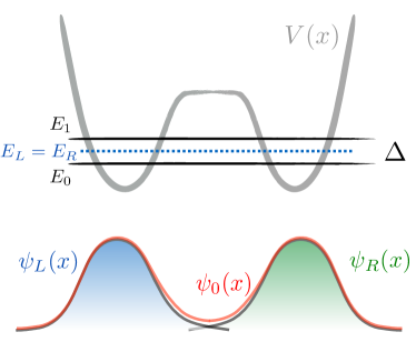
Figure 1: (color online). Cartoon of a double well potential energy $V(x)$ and energy levels. The degenerate levels $E_{L}$ and $E_{R}$ correspond to the localized states $|\psi_{L}\rangle$ (blue) and $|\psi_{R}\rangle$ (green). The degeneracy is lifted by the linear combination of localized states with produce the true eigenstates $\psi_{0}=1/\sqrt{2}(|\psi_{L}\rangle+|\psi_{R}\rangle)$ (red curve) and $\psi_{1}=1/\sqrt{2}(|\psi_{L}\rangle-|\psi_{R}\rangle)$. The tunneling splitting $\Delta$ can be calculated from the overlap of the localized states.

Coherence is easily destroyed by the presence of external noise, as is the case in the proton transfer reactions and in QA. Coupling to an environment can then stop the oscillatory and the transition rate is given by the incoherent tunneling rate, proportional to $\Delta^{2}$.Weiss et al. (1987) This is also the relevant tunneling rate in the adiabatic evolution of quantum annealing (QA), where the annealing time must scale as $\Delta^{-2}$, in order to avoid Landau-Zener diabatic transitions from the ground state to the first excited state.Farhi et al. (2000); Kadowaki and Nishimori (1998)

QMT also appears in QMC simulations, which can be efficient and scale polynomially with system size for quantum many-body problems without a sign problem ( i.e. that the system should obey bosonic statistics or distinguishable particles). Path integral Monte Carlo (PIMC) has been successfully applied to a broad range of continuum and lattice models. In particular PIMC simulationsBerne and Thirumalai (1986); Ceperley (1995a) have addressed problems in which QMT is important, such as proton delocalization in waterCeriotti et al. (2013); Morrone and Car (2008), hydrogenChen et al. (2013) and QA.Santoro et al. (2002); Heim et al. (2015)

PIMC is based on the path integral formalism of quantum mechanics and samples the density matrix corresponding to the quantum Hamiltonian $H$ by means of a classical Hamiltonian $H_{cl}$ on an extended system having an additional dimension, the imaginary time direction. The original quantum system is thus mapped into a classical one, which can be simulated by standard Monte Carlo sampling.

Although QMC techniques are rigorously derived to describe equilibrium properties, we here show that equilibrium PIMC simulations also provide important dynamical quantities, and in particular the the quantum tunneling rate. In Ref. Isakov et al., 2016 we have studied tunneling events in a ferromagnetic Ising model. The Ising ferromagnet can be described by an effective double well model, with the total scalar magnetization as reaction coordinate. We have numerically demonstrated that PIMC tunneling events occur with a rate $k$ which scales, to leading exponential order, as $\Delta^{2}$ – identical to the physical dynamics. We have also seen that with open boundary conditions (OBC) in imaginary time, the tunneling rate can becomes $\Delta$, thus providing a quadratic speed-up.

In this paper we investigate the scaling relation between the PIMC tunneling rate and $\Delta$ for a broader class of problems, of paradigmatic importance in quantum chemistry. We explore models where the effective one-dimensional picture of tunneling should break down.Takada and Nakamura (1994) Our results for continous variables extend the ones for the Ising modelIsakov et al. (2016) and we find that the QMC tunneling rate always follow the $\Delta^{2}$ scaling (or better with OBC). We argue that this is a manifestation of a general phenomenon, that QMC can efficiently simulate the tunneling splitting of the ground state energy levels in multidimensional systems.

II Instantons and QMC

II.1 Path Integral Monte Carlo

PIMC and path integral molecular dynamic (PIMD) techniques directly arise from the Feynman path integral formulation of quantum mechanics and are used to simulate thermodynamic equilibrium. To briefly introduce this approach for continuous space we start from the expression for the partition function $Z$:

$$Z=\int dx\langle x|e^{-\beta H}|x\rangle$$ (1)

where $x$ is the particle position (the generalization to arbitrary dimensions is straightforward), $\beta=1/k_{B}T$ is the inverse temperature and $H$ is the Hamiltonian of the system. Typical real space Hamiltonians are sums of two non-commuting operators $H=\Theta+V$, where $\Theta=1/2m\leavevmode\nobreak\ \partial^{2}/\partial x^{2}$ is the kinetic operator ($m$ being the particle mass), and $V(x)$ is the potential energy. We first notice that the operator $e^{-\beta H}$ corresponds to an evolution in imaginary time $\beta$. We use the Trotter-Suzuki approximation $e^{-\delta_{\tau}(\Theta+V)}\approx e^{-\delta_{\tau}\Theta}e^{-\delta_{\tau}V}$ for small $\delta_{\tau}$.Ceperley (1995a)

Splitting the imaginary time evolution into $P$ small time steps of length $\delta_{\tau}=\beta/P$, the path integral expression for Eq. (1) then becomes

$$Z\propto\int dx_{1}dx_{2}\cdots dx_{P}\exp{\sum_{i=1}^{P}S_{i}}\leavevmode\nobreak\ ,$$ (2)

where $S_{i}=K_{i}+U_{i}$ is the action of each step. $K_{i}=(x_{i-1}-x_{i})^{2}/(2\delta_{\tau}/m)$ is the kinetic part and $U_{i}=\delta_{\tau}/2(V(x_{i-1}-x_{i})$, in the so-called primitive approximation. Notice that $x_{1}=x_{P}$ (closed boundary conditions in imaginary time), for evaluating the trace of the density operator.

This provides an analogy between a quantum system and a classical system with an additional dimension: Eq. (2) is a classical configurational integral and the multidimensional object $(x_{1},\cdots,x_{P-1})\equiv\mathbf{x}(\tau)$ can be viewed as a ring-polymer, whose elements are connected by springs. Each element is labeled by its position along the imaginary time axis, with $0\leq\tau<\beta$. We refer to the Ref. Ceperley, 1995b for a detailed review of path-integrals. An essential feature of Eq. (2) is that the integrand is positive, and hence the distribution $\exp{\sum_{i=1}^{P}S_{i}}$ can be sampled by means of Metropolis Monte Carlo methods or Molecular Dynamics (MD) simulations. The main difference between a pure Monte Carlo vs a MD approach is that the latter samples from the canonical distribution by evolving an appropriate equation of motion, whereas the former uses stochastic Monte Carlo dynamics.

II.2 Instantons in PIMC

Connections between exact quantum dynamics and PIMD approaches, such as Centroid Molecular DynamicsCao and Voth (1993) and Ring Polymer Molecular DynamicsCraig and Manolopoulos (2004) have been discussed Jang et al. (2014); Braams and Manolopoulos (2006); Hele et al. (2015) in the context of real space simulations. Here we follow an alternative approach and summarize the picture of Refs. Isakov et al., 2016; Jiang et al., 2017 based on the instanton theory of tunneling through energy barriers.

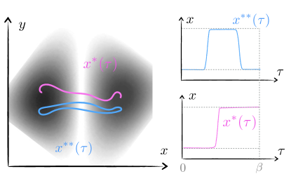
Figure 2: (color online). Left. Cartoon of the typical instantonic paths in configuration space, with PBC, $\mathbf{x}^{**}(\tau)$ (cyan) and OBC in imaginary time, $\mathbf{x}^{*}(\tau)$ (pink). These paths are transition states of the PIMC and PIGS pseudodynamics respectively (in the space of imaginary time trajectories) in double well models (sketched in the grey scale heatmap, see Fig. 6 for a more realistic example). Right. Instantonic trajectories (projected ont ethe reaction cooordinate $x$ axis) as a function of the imaginary time $\tau$. Notice that PIMC instantons have to cross twice the barrier to fulfill the PBC constrain.

In a PIMC or PIMD simulation one samples paths $\mathbf{x}(\tau,t)$ at each update along the simulation time axis $t$, and these paths are distributed according the functional $S(\mathbf{x}(\tau))$ as in Eq. (2). We can define an underlying pseudodynamics used to sample the paths to be given by a first order Langevin dynamics, $\partial\mathbf{x}(\tau,t)/\partial t=-\delta S/\delta\mathbf{x}(\tau,t)+\eta(\tau,t)$. In this case the analogy between quantum statistic and classical statistical mechanics has already been worked out in the stochastic quantization approach in the context of quantum field theory.Parisi et al. (1981) Here, the velocity of the (deformations of) path $\partial\mathbf{x}(\tau,t)/\partial t$ is linked to the generalized force $\delta S/\delta\mathbf{x}(\tau,t)$ and a Gaussian white noise $\eta(\tau,t)$ satisfying the obvious fluctuation-dissipation relation. We can numerically integrate the discretized version of the equation of motion (with time-step $\delta_{t}$), $\mathbf{x}(\tau,t+\delta_{t})=\mathbf{x}(\tau,t)-\delta_{t}\leavevmode\nobreak\ \delta S/\delta\mathbf{x}(\tau,t)+\sqrt{2\delta_{t}}{\bf z}(\tau,t)$, where ${\bf z}(\tau,t)$ is a deformation path, which, after a Trotter discretization is a vector of uniformly random distributed number in the range $[-1,1]$. This defines a Markov chain whose fixed point is the desired distribution, in the $\delta_{t}\rightarrow 0$ limit.

If the system displays two degenerate minima, then the transition state of the pseudodynamics is given by the point $\mathbf{x}_{TS}(\tau)$ satisfying $\delta S(\mathbf{x}_{TS}(\tau))/\delta\mathbf{x}(\tau)=0$ with the condition that $\mathbf{x}_{TS}(\tau)$ is not entirely contained in one of the attraction basins corresponding to the two minimaParisi et al. (1981); Sega et al. (2007); Autieri et al. (2009); Mazzola et al. (2011).

Finding this transition state is generally very complicated, but in the case of a double well potential $V(x)$ it can be done analytically. Here the dominant contribution to the integral comes from the stationary action path $\mathbf{x}^{**}(\tau)$ (determined exactly by the condition $\delta S(\mathbf{x}(\tau))/\delta\mathbf{x}(\tau)=0$) which is called instantonColeman (1977); Forkel (2000); Chudnovsky and Tejada (1998). This trajectory in imaginary time corresponds to a particle moving in the inverted potential $-V(x)$ (see Fig. 2). Following Ref. Isakov et al., 2016 it is possible to evaluate the action $S$ at this point and the amplitude is given by

$$\exp({-S[\mathbf{x}^{*}(\tau)]})\propto\Delta\quad\textrm{(}instanton),$$ (3)

where $\mathbf{x}^{*}(\tau)$ is the open trajectory which connects the two classical turning points under the barrier, near the minima. Notice that, when computing the (diagonal) density matrix $\rho(x)$ periodic boundary conditions (PBC) in imaginary time are required. Now the integral over the closed paths it is dominated by the imaginary time trajectory $\mathbf{x}^{**}(\tau)$ that moves under the barrier starting, reaches the turning point, and returns. Therefore, the saddle point estimation of the integral gives a squared tunneling amplitude

$$\exp({-S[\mathbf{x}^{**}(\tau)]})\propto\Delta^{2}\quad\textrm{(}double\leavevmode\nobreak\ instanton),$$ (4)

due to the cost of creating an instanton and an anti-instanton (see Fig. 2). Returning to the PIMD pseudodynamics, according to Kramers theoryHänggi et al. (1990), the escape rate is $k\propto e^{-S(\mathbf{x}_{TS})}$, and therefore $k\propto\Delta^{2}$ if standard closed path integrals are used, whereas $k\propto\Delta$ if the paths are opened. In Sect. III we extend the study of Ref. Isakov et al., 2016 and demonstrate that the quadratic speedup in the tunneling rate in the case of open boundary path integrals holds also in multi-dimensional continuous space problems.

III One-dimensional double well potential

Let us consider the following one-dimensional double well potential,

$$V(x)=\begin{cases}\lambda(x-x_{0})^{4}-(x-x_{0})^{2},&x\geq x_{0}\\ 0,&-x_{0}\leq x\leq x_{0}\\ \lambda(x+x_{0})^{4}-(x+x_{0})^{2},&x\leq-x_{0}\end{cases}$$ (5)

with $\lambda,x_{0}>0$. We can separately tune the width and the height of the barrier, varying $\lambda$ and $x_{0}$. The height of energy barrier is $\Delta V=1/4\lambda$, and the distance between the two minima is $d=2(x_{0}+\sqrt{1/2\lambda})$ (see inset of Fig. 3) Decreasing $\lambda$ reduces the energy splitting $\Delta$, as the two wells become deeper and more separated. The parameter $x_{0}$ only increases the well separation but doesn’t change the potential energy barrier height. Moreover, a variation of $x_{0}$ leaves the characteristic frequency of the potential wells unchanged, i.e. the kinetic energy associated to the localized states $|\psi_{L}\rangle$ and $|\psi_{R}\rangle$.

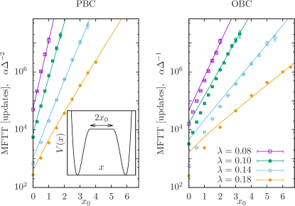
Figure 3: (color online). Average MFTT tunneling time with PIMC (for PBC and OBC) as a function of $x_{0}$ for different values of $\lambda$, at $\beta=20$, corresponding to a temperature always much lower than the barrier height. We use a dimensionless mass parameter $m=1/2$. The inset shows the shape of double well potential $V(x)$, which barrier width (at top) is $2x_{0}$. Notice that for OBC, the measured MFTT is smaller than the one predicted by the $1/\Delta$ formula, when the tunneling rate is large. This happens because both the $\mathbf{x}^{*}(\tau)$ and the $\mathbf{x}^{**}(\tau)$ channel contribute to the tunneling.

Following Ref. Isakov et al., 2016 we measure the mean first tunneling time (MFTT), defined as the number of updates required to find the system in the right well, if the particle has been localized in the left one at the beginning of the simulation. From Fig. 3 we see that the MFTT scales as $1/\Delta^{2}$ when PBC are used, whereas it scales as $1/\Delta$ for OBC, as the parameters $x_{0}$ and $\lambda$ change. The gap $\Delta$ is obtained using a discrete variable representation (DVR) techniqueColbert and Miller (1992). This scaling relation holds for PIMC with local Metropolis updates and PIMD (using both first and second order Langevin thermostats), at large $\beta$, and in the limit of small time steps $\delta_{\tau},\delta_{t}\textrm{(for PIMD)}\rightarrow 0$ limit. This means that the scaling of tunneling rate in a double well model $k\propto\Delta^{2}$ is correctly reproduced.Weiss et al. (1987).

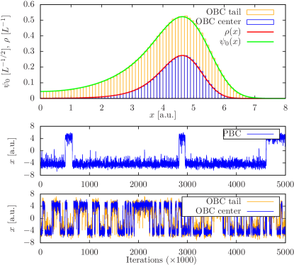
Figure 4: (color online). Top panel: position distributions (histograms) obtained considering the center (blue) or the tail (orange) of the OBC path. The distributions are area-normalized respectively with the exact $\rho(x)\approx|\psi_{0}|^{2}$ distribution (red) and the exact ground state $\psi_{0}(x)$ (green). We plot only for $x>0$ and we use $x_{0}=3$ and $\lambda=0.14$ in Eq. (5). The difference between the sampled distributions and the reference ones are negligible. We perform simulations at low temperatures, $\beta=20\gg\Delta V$. Middle and lower panel: the position of the particle as the simulation progresses for PBC and OBC (both for center and tail). As expected the tunneling rate is much larger for OBC.

Why do the open paths tunnel faster from the point of view of PIMC pseudodynamics? To answer this question we first observe that, for sufficiently low temperatures, the center of the open-path $\mathbf{x}^{*}(\tau\approx\beta/2)$ sample from the ground state distribution $|\psi_{0}(x)|^{2}$, whereas the tails, $\mathbf{x}^{*}(\tau\approx 0)$ and $\mathbf{x}^{*}(\tau\approx\beta)$, sample from the ground state distribution $\psi_{0}(x)$. Therefore the tails spend more time inside the barrier (see Fig. 4) compared to the center, which follows instead the more localized $\psi_{0}^{2}$ distribution. Once that one of the two tails crosses the barrier, then the rest of the open-polymer may easily follow, so that the whole polymer ”tunnel” faster compare to its PBC counterpart. This also means that, with OBC, it is possible to sample from the equilibrium distribution $\rho(x)\approx|\psi_{0}|^{2}$, using the center of the path, while having a considerable speed-up in the sampling. We notice that this feature is not surprising as the OBC technique is closely related to the so called path integral ground stateSarsa et al. (2000) (PIGS) technique. Indeed, in the PIGSSarsa et al. (2000) approach, sampling from the tails gives the mixed distribution $\psi_{0}(x)\psi_{T}(x)$, but in our case the trial wavefunction is $\psi_{T}(x)=1$. Therefore, we propose that OBC should be used not only in the context of quantum annealing but much more broadly also in material simulations, as far as low-temperature conditions are investigated.

IV Multidimensional tunneling

The double well model provided in Sect. III is a prototypical example of one-dimensional tunneling. One could argue that, despite having many-spins degrees of freedom, the spin models investigated in Ref. Isakov et al., 2016 are also effectively one-dimensional models, as the relevant reaction coordinate is the total scalar magnetization $M$. Indeed the instantonic nature of the transition state can be seen if we plot $M(\tau)$ as a function of the imaginary time parameter $\tau$.

It is much more straightforward to devise models that require multidimensional tunneling in continuos space, rather than spin models.Stella et al. (2006a); Inack and Pilati (2015) To this end we borrow insights from quantum chemistry, where simplified model for characterizing proton tunneling have been devised.Auerbach and Kivelson (1985); Makri and Miller (1987); Takada and Nakamura (1994); Nakamura and Mil’nikov (2013) In particular in Ref. Takada and Nakamura, 1994 a semiclassical theory of multidimensional tunneling is formulated, unraveling its qualitative differences compared to one-dimensional tunneling. It was found that in multidimensional tunneling two regimes can be identified: the pure tunneling case, which is effectively one-dimensional, where the tunneling path can be defined uniquely, and the mixed tunneling regime when tunneling occurs very broadly, i.e. where a set of dominant semiclassical paths $\{{\bf x}_{TS}\}$ is not defined. In the first case, the action which defines the semiclassical wavefunction is purely imaginary, whereas in the latter the action is complex. We refer the interested reader to Ref. Takada and Nakamura, 1994 for the analytical details.

Investigating QMC simulations for such mixed tunneling models, where the QMC scaling relation with the exact QMT rate might be expected to break down, we instead find that the quantum tunneling rate given by QMC scales as the adiabatic quantum evolution also in this case.

IV.1 QMC tunneling rate scaling

We first consider the simple shifted parabola bidimensional model of Ref. Takada and Nakamura, 1994, which is a minimal model for the antisymmetric mode coupling mechanism for proton tunneling in malonaldehyde, a well-studied molecular test case. The Hamiltonian reads

$$H=\Theta+V_{A}\leavevmode\nobreak\ ,$$ (6)

with

$$\Theta=-{g^{2}\over 2}\left({\partial^{2}\over\partial x^{2}}+{\partial^{2}\over\partial y^{2}}\right)\leavevmode\nobreak\ ,$$ (7)

where $g>0$ is a dimensionless parameter which sets the strength of the quantum fluctuations. The potential is

$$V_{A}(x,y)=\begin{cases}\frac{1}{2}(x+1)^{2}+\frac{1}{2}\omega_{y}^{2}(y+y_{0})^{2},&x<0\\ \frac{1}{2}(x-1)^{2}+\frac{1}{2}\omega_{y}^{2}(y-y_{0})^{2},&x\geq 0\leavevmode\nobreak\ ,\end{cases}$$ (8)

where $y_{0}>0$ and $\omega_{y}^{2}>0$ are dimensionless harmonic potential parameters. This potential represents two parabolas, located respectively in the half-planes $x<0$ and $x>0$, with centers shifted along the $y$-axis by an amount $2y_{0}$. In the case of malonaldehyde molecule, the coordinate $x$ represents the motion of transferring the proton, while $y$ represents the C–O stretching mode. The sign of $a^{2}=y_{0}^{2}-g/\omega_{y}$, distinguishes between the two ground state QMT cases: pure tunneling for $a^{2}>0$ and mixed tunneling for $a^{2}<0$.

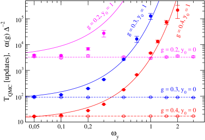
Figure 5: (color online). Average MFTT tunneling time with PIMC (with PBC) as a function of $\omega_{y}$ for different values of $g=0.2,0.3,0.4$ (pink, blue and red data series respectively) and two values of $y_{0}=0$ (empty symbols) and $1$ (full symbols). The potential considered is $V_{A}$ as in Eq. 8. Lines represent fit to the exact $\Delta^{-2}$ gap values, obtained with the DVR method. The proportionality constant $\alpha(g)$ which multiplies the inverse gap squared is different for each $g$ value, and fitted using only the $y_{0}=0$ data series. Notice the logarithmic scale on both axis.

In Fig. 5 we present results of PIMC simulations with local updates, using PBC, at large $\beta$ (very low temperature), and in the converged time step $\delta_{\tau}\rightarrow 0$ limit, to describe faithfully ground state tunneling. The path deformations are obtained by displacing each bead at a time by an amout $(dx,dy)$. The displacements are Gaussian distributed with zero mean and the variance is tuned in order to obtain a Metropolis acceptance probability of $\approx 40\%$.

Again we study the MFTT obtained with PIMC simulations as a function of the parameter $\omega_{y}$, in the range $[0.05,2]$ and for three different choices of $g=0.2,0.3,0.4$, and for two shifting values $y_{0}=0$ and $1$. Following Ref. Isakov et al., 2016 we define the MFTT as the number of PIMC updates required to observe an instantonic state. In turn, we algorithmically define an instanton path, as spending approximately the same fraction of imaginary time in either well.

With these parameters ranges we can roughly mimic proton transfer reactions in malonaldehyde.Makri and Miller (1987) For this molecule, it is found that, if the tunneling is described only by a one-dimensional process, the tunneling rate is reduced by two orders of magnitude compared to experimental and recent theoretical valuesBosch et al. (1990); Cvitaš and Althorpe (2016). Furthermore, it was argued in Ref. Takada and Nakamura, 1994 that deviations from the one dimensional picture leads to a mixed tunneling regime where no well defined tunneling path exists. Therefore it could be possible that QMC underestimates the exact tunneling rate. In the context of quantum annealing problem, this might mean that the performances of QA and its simulated version through QMC could be very different, under these “mixed tunneling” conditions.

We first perform tests for $y_{0}=0$, where we are always in the regime $a^{2}<0$ , i.e. the mixed tunneling regime. The gap $\Delta$ is constant as a function of $\omega_{y}$, and we observe the same in QMC, where the MFTT remains constant. Its precise value depends on the parameter $g$. We use these data to fix the proportionality constant $\alpha(g)$, which we use later to compare the MFTT to the value $\alpha(g)\Delta^{-2}$. Notice that in the $\omega_{y}\rightarrow 0$ limit the two wells become parallel and indefinitely extended along the $y$ direction. In this limit, we observe an infinite number of tunneling paths that connects reactants on left well with the products on the right.

Next, we set $y_{0}=1$ and repeat the simulations. This time the scaling of $\Delta^{-2}$ as a function of $\omega_{y}$ is non-trivial. Nevertheless it approaches the previous value – for any given $g$ – in the $\omega_{y}\rightarrow 0$ limit, as the two wells are infinitely long and the shift given by $y_{0}$ becomes irrelevant. In this case, we cross the transition point $a^{2}=0$ between the the two regimes of tunneling, when $\omega_{y}=g$. We still observe a satisfactorily agreement between the QMC MFTT data series and the $\alpha(g)\Delta^{-2}$ functions. While a residual difference between the QMC data and the expected $\Delta^{-2}$ behaviour can now be appreciated, this difference is small over the broad $\omega_{y}$-range investigated, i.e. nowhere near the 2 order of magnitude worst case scenario, reported in Ref. Bosch et al., 1990. We note that in Ref. Bosch et al., 1990 the full multidimensional problem is reduced to a one-dimensional calculation. This is the origin of the observed large deviation from the theoretical value. Notice also that, once we fix the constant $\alpha(g)$ the QMC tunneling time is always smaller than $\alpha(g)\Delta^{-2}$, so QMC tunnels slightly more efficiently than QA, even with PBC.

IV.2 QMC reaction pathways and fluctuations around the instanton solution

In this Section we explicitly track the QMC pseudo-dynamics transition states and compare to the instantonic trajectory computed by minimizing the action $S$. Let us consider the symmetric mode coupling potential,

$$V_{S}(x,y)=\frac{1}{8}(x-1)^{2}(x+1)^{2}+{\omega_{y}^{2}\over 2}\left(y+{\gamma\over\omega_{y}^{2}}(x^{2}+1)\right)^{2}\leavevmode\nobreak\ .$$ (9)

This potential energy surface is continuos and has been widely used as a model for proton tunneling. In the typical example of malonaldehyde, the coordinate $x$ represents the motion of the proton transferring between the Oxigen atoms, while $y$ gives the scissors-like motion of the O-C-C-C-O frameTakada and Nakamura (1994). We use the dimensionless potential parameters $(\omega_{y},\gamma,g)=(0.48,0.39,0.10)$ to fit the model to the ab-initio potential energy surfaceBosch et al. (1990). In this way we can directly compare the transition paths given by the PIMC simulation with other techniques, such as the Ring Polymer Instanton (RPI) method,Richardson and Althorpe (2011); Richardson et al. (2011); Cvitaš and Althorpe (2016); Richardson et al. (2016) recently introduced to calculate energy splitting. In the RPI framework, one first needs to locate the saddle point of the action $S$ (the instanton), and then evaluates the splitting energy by computing the functional integral up to second order in the fluctuations around the dominant contribution. This approach employs neither PIMC sampling nor PIMD, as the instanton path is obtained via action’s minimization and the initial guess is an OBC path that already connects the reactant to product state.

In Fig. 6 we plot a sample of transition paths produced by the PIMC pseudodynamics and recognize their instantonic character. We compare some OBC transition paths sampled with our PIMC simulation, against the RPI solution recently published in Ref. Cvitaš and Althorpe, 2016. We see that these instanton paths form a bundle around the RPI saddle point solution, and are qualitatively distant from the minimum energy path (MEP), which would be typical of a classical thermally activated processCvitaš and Althorpe (2016). It is remarkable that a simple PIMC simulation obtains the instanton path, which is otherwise computed only by a complex minimization procedure as in the RPI scheme.

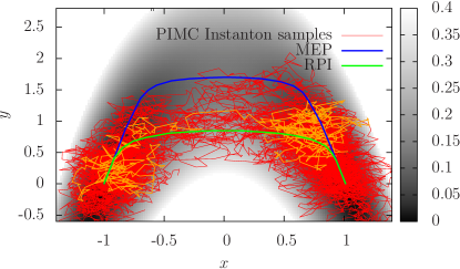
Figure 6: (color online). Heat map plot of the two-dimensional model potential $V_{S}(x,y)$ of malonaldehyde of Eq. 9. Red lines represents a collection of $20$ instanton paths sampled with PIMC. These samples are uncorrelated as they correspond to independent tunneling events after full reinitialization of the starting path in the reactant well, i.e. when the MFTT identification criteria are met (see text) we stop the PIMC simulation and collect the last path which has been generated. We use a sufficiently large inverse temperature $\beta=400$, $P=512$ Trotter slices and OBC in imaginary time. We single out, in orange, one of these instances, in order to appreciate their instantonic character. Indeed most of the Trotter slices are located at the bottom of the two wells, and only very few of them on the barrier (cfn. Fig. 2), these correspond to the middle of the imaginary time trajectory ($\tau\approx\beta/2$). The PIMC instanton paths are not smooth, given the large number of Trotter slices, and represent themselves fluctuations around an average transition path, qualitatively very close to the RPI solution taken from Ref. Cvitaš and Althorpe, 2016 (green, see text). We also plot the MEP (blue) for comparison. The proton tunneling paths typically take place on a region quite far from the saddle point $(0,\gamma/\omega_{y}^{2}\approx 1.7)$ of the potential.

Another advantage of PIMC is that we can directly sample the statistical fluctuations around the dominant solution $\mathbf{x}^{*}(\tau)$. To second order the action can be expanded as Parisi et al. (1981)

$$S \simeq S[\mathbf{x}^{*}]+\frac{1}{2}\int_{0}^{\beta}d\tau^{\prime}\int_{0}^{\beta}d\tau^{\prime\prime}\frac{\delta^{2}S[\mathbf{x}^{*}]}{\delta\mathbf{x}(\tau^{\prime})\delta\mathbf{x}(\tau^{\prime\prime})}\mathbf{y}(\tau)\mathbf{y}(\tau)$$

$$\simeq S[\mathbf{x}^{*}]+\frac{1}{2}\int_{0}^{\beta}d\tau\leavevmode\nobreak\ \leavevmode\nobreak\ \mathbf{y}(\tau)\hat{G}[\mathbf{x}^{*}]\mathbf{y}(\tau),$$ (10)

where $\mathbf{y}(\tau)$ is a fluctuation path, satisfying $\mathbf{y}(0)=\mathbf{y}(\beta)=\mathbf{0}$, and $\hat{G}=-\frac{d^{2}}{d\tau^{2}}+V^{\prime\prime}[\mathbf{x}^{*}]$ is the fluctuation operator, or Hessian, adopting the notation of Ref. Richardson and Althorpe, 2011. Here $V^{\prime\prime}[\mathbf{x}^{*}]$ is the second derivative of the potential computed along the instanton path $\mathbf{x}^{*}(\tau)$.

In practice one always deals with discretized trajectories in imaginary time. Therefore also the operator $\hat{G}$ is discretized using finite differences and then diagonalized to obtain the normal modes and frequency of the fluctuations. The resulting product of Gaussian integrals allows one to evaluate Eq. IV.2.

However, it could be cumbersome to evaluate $G$ for ab-initio potentials (as they require evaluation of second derivaties of the potential), or in the case of rugged energy landscapes, where local curvature at the saddle point $V^{\prime\prime}[\mathbf{x}^{*}]$ does not correctly represent the actual amplitude of the quantum fluctuationsFaccioli ; Mazzola et al. (2011). On the other hand, the inverse operator $G^{-1}$ can be computed stochastically with PIMC, using the relation

$$\hat{G}^{-1}[\mathbf{x}^{*}](\tau_{1},\tau_{2})=\langle\mathbf{y}(\tau_{1})\mathbf{y}(\tau_{2})\rangle_{\mathbf{x}^{*}},$$ (11)

where the right hand side denotes the statistical average of the fluctuations, around a given path $\mathbf{x}^{*}$. This approach gives a more effective and fast estimate of the curvature of the potential surface in the above cases.

We note that PIMC sampling techniques have already been used to compute tunneling splittings in molecular and condensed matter systemsKuki and Wolynes (1987); Ceperley and Jacucci (1987); Alexandrou and Negele (1988); Mátyus et al. (2016). Here we propose an alternative and simple way to compute ratios of quantum mechanical rate constants. Suppose that the potential displays several minima, i.e. that we have one reactant state $R$ and two, or more, possible product states $P_{1},P_{2}$. By computing the ratio of the average PIMC tunneling times, with OBC, required to perform the transitions $R\rightarrow P_{1}$ and $R\rightarrow P_{2}$ respectively, we can estimate the ratio of the tunneling splittings $\Delta_{R,P_{2}}/\Delta_{R,P_{1}}$ corresponding to the two quantum mechanical transitions, provided that enough statistics of instanton events can be gathered in a reasonable amount of time. This approach is predictive, as the instantons are generated by the PIMC pseudodynamics, without any a-priori knowledge of the final product state.

This problem is closely connected with quantum annealing, where, starting from some high energy “reactant” states $R$’s, one would like to reach the “product” state $P_{i}$ having the lowest possible potential energy, after a sequence of tunneling eventsKnysh (2016). The relative probability of finding this state, compared to other metastable ones, is well described by PIMC simulations.

V Conclusions

We have studied the tunneling of path integral based equilibrium simulations in continuos space models, generalizing a previous studyIsakov et al. (2016) on ferromagnetic spin models. We demonstrates that the PIMC tunneling rate scales as a $\Delta^{2}$ if periodic boundary conditions in imaginary time are used, while it scales as $\Delta$ with open boundary conditions. These scaling relations seem to be a general property of path integral methods, as long as reasonable semi-local updates are employed during the Markov chain pseudodynamics (see Sect. II.2). In this case, in double well potentials, it is possible to directly identify the transition state of the path integral pseudodynamics –a purely classical process– and therefore compute its classical reaction rate using Kramers theory.

This transition state is the instanton path, and we remark here that this trajectory is sampled by the PIMC pseudodynamics using local updates, i.e. we don’t need to engineer such kind of global update moves as in Refs. Stella et al., 2006b; Alexandrou and Negele, 1988. Indeed the latter approach would invalidate the premises and discussions presented in this paper and artificially increase the reaction rate observed with PIMC. On the other hand, building in instantonic updates in the Metropolis procedure requires a full knowledge of the system, i.e. knowing in advance the transition states. Having this knowledge one would solve beforehand the quantum annealing problem, for example, without even running any PIMC simulation.

The quadratic speed-up in tunneling efficiency is a robust feature of OBC simulations for tunneling through individual barriers. In the context of simulations, therefore, we propose that open path integral simulations should be used instead of PBC and will accelerate the sampling, whenever ground state properties are desired.

We also turned our attention to simplified models for proton transfer, where multidimensional tunneling is deemed to be important, and a semiclassical description of tunneling as an effective one-dimensional process has been seen to fail. Nevertheless, the scaling relation of the PIMD transition rate, compared to the exact incoherent tunneling rate $\Delta^{2}$ holds also in this case.

The above finding is very interesting because often in a multidimensional potential the smooth tunneling path (instanton) connecting the minima of the potential does not exists due to the effects of a so-called dynamical tunneling Huang et al. (1990); Takada and Nakamura (1994); Zamastil (2005); Razavy (2013). The lack of an instanton path was also studied, e.g., in the case of the two-dimensional shifted parabola model Ref. Takada and Nakamura, 1994 considered in our study. On the other hand, as explained above in Sec.  II.2 based on the Kramers theory arguments, the existence of the instanton path is a key requirement that leads to the identical QMT and PIMC scaling laws.

To explain this conundrum we observe that the difficulty with instanton description in the case of a tunneling in a multidimensional potential usually occurs when one needs to match the solutions given by Wentzel–Kramers–Brillouin (WKB) theory in classically allowed and forbidden regions at the boundary formed by caustics. Caustics result in the complex (oscillatory) behavior of the wavefunction under the barrier Huang et al. (1990); Takada and Nakamura (1994); Zamastil (2005). This oscillatory behavior results in a phase problem in QMC.

We argue that at zero temperature this situation does not occur generically, because a classically allowed region in configuration space “collapses” into the point corresponding to the minimum of the potential. As usually, to study tunneling one should consider the wavefunction under the barrier that nearly coincides with the ground state wavefunction near one of the minima of $V$, exponentially decaying away from it. The mechanical action $S[{\bf x}(\tau)]=\int_{\infty}^{\tau}(m\dot{\bf x}^{2}(\tau_{1})+V({\bf x}(\tau_{1})))d\tau_{1}$ for the wavefunction is associated with the unstable Lagrangian manifold Guckenheimer and Holmes (2013) formed by real-valued trajectories $({\bf x}(\tau),{\bf p}(\tau))$ in the phase space moving in the imaginary time $\tau$ in the inverted potential $-V$ (above ${\bf p}(\tau)$ is a system momentum). The trajectories emanate at time $t=-\infty$ from the corresponding maximum of the $-V$. In general, projections of the Lagrangian manifold onto the coordinate space ${\bf x}$ can have caustics, cusps (and more complex singularities in the dimensions higher then twoArnold (1989)) in classically forbidden region. These singularities lead to multi-valuedness of the action surface and some of its branches become complex. However the minimum action surface is real- and single-valued. It possesses lines where the surface gradient is discontinuous (see Fig. 7) They correspond to the so-called switching lines in configuration space Dykman et al. (1994). Points at different sides of the switching are reached by a topologically different imaginary-time paths as shown in Fig. 7(b). Therefore any point ${\bf x}$ can be reached by the most-probable path that provides the minimum of the action and never crosses a switching line. An instanton is a particular member of the minimum-action family of paths that connects the two maxima of the potential $-V$. It corresponds to the heteroclinic orbit (${\bf x}^{*}(\tau)$ ,${\bf p}^{*}(\tau)$) contained in the unstable Lagrangian manifold shared by the two maxima Ref. Sharpee et al., 2002. This explains why ground state tunneling splitting for the particle in a multidimensional potential is always described by the instanton with a real-valued action and therefore can be simulated efficiently by PIMC.

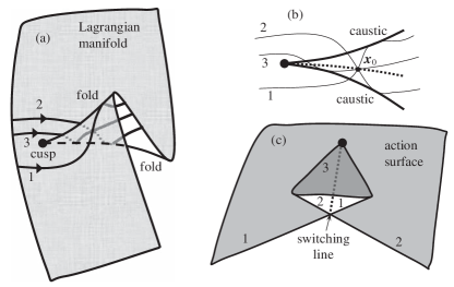
Figure 7: (a) Unstable manifold with a cusp singularity and three typical imaginary-time paths emanating from one of the minima of the potential. (b) Projection of the unstable manifold onto the coordinate plane ($X_{1},X_{2}$) . The two folds project onto caustics, while projections of the three trajectories intersect at the point $X_{0}$ that lies on the switching line showed as dashed. (c) The action $S(X_{0})$ is a three valued function in between the caustics. Two of its lower branches intersect along the switching line. After Refs.  Kamenev, 2011; Dykman et al., 1994.

This confirms that PIMC simulation of QMT in the ground state can be done without any loss of efficiency compared to what real system would do. The fact that PIMC simulations have the same scaling with the problem size as physical quantum annealing was recently experimentally confirmed, again on a spin system on chimera graphDenchev et al. (2016). In this context, it is unlikely that QA to find a ground state of optimization problem can achieve an exponential speedup over classical computation, only by using QMT as a computational resource.

We remark here that these conclusions hold only when so-called stoquastic Hamiltonians are used, i.e. Hamiltonians which allow PIMC simulations. This is the case of the Hamiltonians used in this paper. In most reaction simulations protons are assumed to be distinguishable particles, and, in QA the standard transverse field Ising Hamiltonian is also stoquastic.Johnson et al. (2011); Bunyk et al. (2014) This provides additional evidences that QA machines should implement non-stoquastic Hamiltonians which display sign-problem,Seki and Nishimori (2012); Mazzola and Troyer (2017); Hormozi et al. (2016) to avoid efficient simulations by QMC methods.

Acknowledgements. GM acknowledges useful discussions with P. Faccioli, S. Sorella and G.E. Santoro. MT acknowledges hospitality of the Aspen Center for Physics, supported by NSF grant PHY-1066293. Simulations were performed on resources provided by the Swiss National Supercomputing Centre (CSCS). This work was supported by the European Research Council through ERC Advanced Grant SIMCOFE by the Swiss National Science Foundation through NCCR QSIT and NCCR Marvel. This paper is based upon work supported in part by ODNI, IARPA via MIT Lincoln Laboratory Air Force Contract No. FA8721-05-C-0002. The views and conclusions contained herein are those of the authors and should not be interpreted as necessarily representing the official policies or endorsements, either expressed or implied, of ODNI, IARPA, or the U.S. Government. The U.S. Government is authorized to reproduce and distribute reprints for Governmental purpose not-withstanding any copyright annotation thereon.

References

- Nagel and Klinman (2006) Zachary D Nagel and Judith P Klinman, “Tunneling and dynamics in enzymatic hydride transfer,” Chemical reviews 106, 3095–3118 (2006).
- Bell (2013) Ronald Percy Bell, The tunnel effect in chemistry (Springer, 2013).
- Zuev et al. (2003) Peter S Zuev, Robert S Sheridan, Titus V Albu, Donald G Truhlar, David A Hrovat, and Weston Thatcher Borden, “Carbon tunneling from a single quantum state,” Science 299, 867–870 (2003).
- Nakamura and Mil’nikov (2013) Hiroki Nakamura and Gennady Mil’nikov, Quantum mechanical tunneling in chemical physics (CRC Press, 2013).
- Ceriotti et al. (2016) Michele Ceriotti, Wei Fang, Peter G Kusalik, Ross H McKenzie, Angelos Michaelides, Miguel A Morales, and Thomas E Markland, “Nuclear quantum effects in water and aqueous systems: Experiment, theory, and current challenges,” Chemical reviews (2016).
- Richardson et al. (2016) Jeremy O Richardson, Cristóbal Pérez, Simon Lobsiger, Adam A Reid, Berhane Temelso, George C Shields, Zbigniew Kisiel, David J Wales, Brooks H Pate, and Stuart C Althorpe, “Concerted hydrogen-bond breaking by quantum tunneling in the water hexamer prism,” Science 351, 1310–1313 (2016).
- Bonev et al. (2004) Stanimir A Bonev, Eric Schwegler, Tadashi Ogitsu, and Giulia Galli, “A quantum fluid of metallic hydrogen suggested by first-principles calculations,” Nature 431, 669–672 (2004).
- Pickard and Needs (2007) Chris J. Pickard and Richard J. Needs, “Structure of phase III of solid hydrogen,” Nature Physics 3, 473–476 (2007).
- Dalladay-Simpson et al. (2016) Philip Dalladay-Simpson, Ross T Howie, and Eugene Gregoryanz, “Evidence for a new phase of dense hydrogen above 325 gigapascals,” Nature 529, 63–67 (2016).
- Mazzola and Sorella (2017) Guglielmo Mazzola and Sandro Sorella, “Accelerating ab initio molecular dynamics and probing the weak dispersive forces in dense liquid hydrogen,” Phys. Rev. Lett. 118, 015703 (2017).
- Johnson et al. (2011) MW Johnson, MHS Amin, S Gildert, T Lanting, F Hamze, N Dickson, R Harris, AJ Berkley, J Johansson, P Bunyk, et al., “Quantum annealing with manufactured spins,” Nature 473, 194–198 (2011).
- Bunyk et al. (2014) P. I. Bunyk, E. M. Hoskinson, M. W. Johnson, E. Tolkacheva, F. Altomare, A. J. Berkley, R. Harris, J. P. Hilton, T. Lanting, A. J. Przybysz, and J. Whittaker, “Architectural considerations in the design of a superconducting quantum annealing processor,” IEEE Transactions on Applied Superconductivity 24, 1–10 (2014).
- Farhi et al. (2000) Edward Farhi, Jeffrey Goldstone, Sam Gutmann, and Michael Sipser, “Quantum computation by adiabatic evolution,” arXiv preprint quant-ph/0001106 (2000).
- Kadowaki and Nishimori (1998) Tadashi Kadowaki and Hidetoshi Nishimori, “Quantum annealing in the transverse ising model,” Phys. Rev. E 58, 5355–5363 (1998).
- Farhi et al. (2001) Edward Farhi, Jeffrey Goldstone, Sam Gutmann, Joshua Lapan, Andrew Lundgren, and Daniel Preda, “A quantum adiabatic evolution algorithm applied to random instances of an np-complete problem,” Science 292, 472–475 (2001).
- Das and Chakrabarti (2008) Arnab Das and Bikas K. Chakrabarti, “Colloquium : Quantum annealing and analog quantum computation,” Rev. Mod. Phys. 80, 1061–1081 (2008).
- Crosson and Harrow (2016) Elizabeth Crosson and Aram W Harrow, “Simulated quantum annealing can be exponentially faster than classical simulated annealing,” in Foundations of Computer Science (FOCS), 2016 IEEE 57th Annual Symposium on (IEEE, 2016) pp. 714–723.
- Boixo et al. (2016) Sergio Boixo, Vadim N Smelyanskiy, Alireza Shabani, Sergei V Isakov, Mark Dykman, Vasil S Denchev, Mohammad H Amin, Anatoly Yu Smirnov, Masoud Mohseni, and Hartmut Neven, “Computational multiqubit tunnelling in programmable quantum annealers,” Nature communications 7 (2016).
- Weiss et al. (1987) Ulrich Weiss, Hermann Grabert, Peter Hänggi, and Peter Riseborough, “Incoherent tunneling in a double well,” Physical Review B 35, 9535 (1987).
- Berne and Thirumalai (1986) Bruce J Berne and D Thirumalai, “On the simulation of quantum systems: path integral methods,” Annual Review of Physical Chemistry 37, 401–424 (1986).
- Ceperley (1995a) David M Ceperley, “PATH-INTEGRALS IN THE THEORY OF CONDENSED HELIUM,” Reviews Of Modern Physics 67, 279–355 (1995a).
- Ceriotti et al. (2013) Michele Ceriotti, Jérôme Cuny, Michele Parrinello, and David E Manolopoulos, “Nuclear quantum effects and hydrogen bond fluctuations in water,” Proceedings of the National Academy of Sciences 110, 15591–15596 (2013).
- Morrone and Car (2008) Joseph A. Morrone and Roberto Car, “Nuclear quantum effects in water,” Phys. Rev. Lett. 101, 017801 (2008).
- Chen et al. (2013) Ji Chen, Xin-Zheng Li, Qianfan Zhang, Matthew IJ Probert, Chris J Pickard, Richard J Needs, Angelos Michaelides, and Enge Wang, “Quantum simulation of low-temperature metallic liquid hydrogen,” Nature communications 4 (2013).
- Santoro et al. (2002) Giuseppe E. Santoro, Roman Martonak, Erio Tosatti, and Roberto Car, “Theory of quantum annealing of an ising spin glass,” Science 295, 2427–2430 (2002).
- Heim et al. (2015) Bettina Heim, Troels F. Rønnow, Sergei V. Isakov, and Matthias Troyer, “Quantum versus classical annealing of ising spin glasses,” Science 348, 215–217 (2015).
- Isakov et al. (2016) Sergei V. Isakov, Guglielmo Mazzola, Vadim N. Smelyanskiy, Zhang Jiang, Sergio Boixo, Hartmut Neven, and Matthias Troyer, “Understanding quantum tunneling through quantum monte carlo simulations,” Phys. Rev. Lett. 117, 180402 (2016).
- Takada and Nakamura (1994) Shoji Takada and Hiroki Nakamura, “Wentzel-Kramers-Brillouin theory of multidimensional tunneling: General theory for energy splitting,” The Journal of Chemical Physics 100, 98–113 (1994).
- Ceperley (1995b) D. M. Ceperley, “Path integrals in the theory of condensed helium,” Rev. Mod. Phys. 67, 279–355 (1995b).
- Cao and Voth (1993) Jianshu Cao and Gregory A. Voth, “A new perspective on quantum time correlation functions,” The Journal of Chemical Physics 99, 10070–10073 (1993).
- Craig and Manolopoulos (2004) Ian R. Craig and David E. Manolopoulos, “Quantum statistics and classical mechanics: Real time correlation functions from ring polymer molecular dynamics,” The Journal of Chemical Physics 121, 3368–3373 (2004).
- Jang et al. (2014) Seogjoo Jang, Anton V. Sinitskiy, and Gregory A. Voth, “Can the ring polymer molecular dynamics method be interpreted as real time quantum dynamics?” The Journal of Chemical Physics 140, 154103 (2014), http://dx.doi.org/10.1063/1.4870717.
- Braams and Manolopoulos (2006) Bastiaan J. Braams and David E. Manolopoulos, “On the short-time limit of ring polymer molecular dynamics,” The Journal of Chemical Physics 125, 124105 (2006), http://dx.doi.org/10.1063/1.2357599.
- Hele et al. (2015) Timothy J. H. Hele, Michael J. Willatt, Andrea Muolo, and Stuart C. Althorpe, “Communication: Relation of centroid molecular dynamics and ring-polymer molecular dynamics to exact quantum dynamics,” The Journal of Chemical Physics 142, 191101 (2015), http://dx.doi.org/10.1063/1.4921234.
- Jiang et al. (2017) Zhang Jiang, Vadim N. Smelyanskiy, Sergei V. Isakov, Sergio Boixo, Guglielmo Mazzola, Matthias Troyer, and Hartmut Neven, “Scaling analysis and instantons for thermally assisted tunneling and quantum monte carlo simulations,” Phys. Rev. A 95, 012322 (2017).
- Parisi et al. (1981) Georgio Parisi, Yong-shi Wu, et al., “Perturbation theory without gauge fixing,” Scientia Sinica 24, 483–469 (1981).
- Sega et al. (2007) M Sega, P Faccioli, F Pederiva, G Garberoglio, and H Orland, “Quantitative protein dynamics from dominant folding pathways,” Physical Review Letters 99, 118102 (2007).
- Autieri et al. (2009) E Autieri, P Faccioli, M Sega, F Pederiva, and H Orland, “Dominant reaction pathways in high-dimensional systems,” The Journal of chemical physics 130, 064106 (2009).
- Mazzola et al. (2011) Guglielmo Mazzola, Silvio a Beccara, Pietro Faccioli, and Henri Orland, “Fluctuations in the ensemble of reaction pathways,” The Journal of chemical physics 134, 164109 (2011).
- Coleman (1977) Sidney Coleman, “Fate of the false vacuum: Semiclassical theory,” Phys. Rev. D 15, 2929 (1977).
- Forkel (2000) H. Forkel, “A Primer on Instantons in QCD,” ArXiv High Energy Physics - Phenomenology e-prints (2000), hep-ph/0009136 .
- Chudnovsky and Tejada (1998) E. M. Chudnovsky and J. Tejada, Macroscopic Quantum Tunneling of the Magnetic Moment (Cambridge, UK: Cambridge University Press, 1998).
- Hänggi et al. (1990) Peter Hänggi, Peter Talkner, and Michal Borkovec, “Reaction-rate theory: fifty years after kramers,” Reviews of modern physics 62, 251 (1990).
- Colbert and Miller (1992) Daniel T Colbert and William H Miller, “A novel discrete variable representation for quantum mechanical reactive scattering via the s-matrix kohn method,” The Journal of chemical physics 96, 1982–1991 (1992).
- Sarsa et al. (2000) A. Sarsa, K. E. Schmidt, and W. R. Magro, “A path integral ground state method,” J. Chem. Phys. 113, 1366–1371 (2000).
- Stella et al. (2006a) Lorenzo Stella, Giuseppe E. Santoro, and Erio Tosatti, “Monte carlo studies of quantum and classical annealing on a double well,” Phys. Rev. B 73, 144302 (2006a).
- Inack and Pilati (2015) EM Inack and S Pilati, “Simulated quantum annealing of double-well and multiwell potentials,” Physical Review E 92, 053304 (2015).
- Auerbach and Kivelson (1985) Assa Auerbach and S Kivelson, “The path decomposition expansion and multidimensional tunneling,” Nuclear Physics B 257, 799–858 (1985).
- Makri and Miller (1987) Nancy Makri and William H. Miller, “Basis set methods for describing the quantum mechanics of a “system” interacting with a harmonic bath,” The Journal of Chemical Physics 86, 1451–1457 (1987).
- Note (1) The actual value would be , here we artificially enhance in order to increase the observed tunneling rate.
- Bosch et al. (1990) Enric Bosch, Miquel Moreno, José M. Lluch, and Juan Bertrán, “Bidimensional tunneling dynamics of malonaldehyde and hydrogenoxalate anion. a comparative study,” The Journal of Chemical Physics 93, 5685–5692 (1990).
- Cvitaš and Althorpe (2016) Marko T Cvitaš and Stuart C Althorpe, “Locating instantons in calculations of tunneling splittings: The test case of malonaldehyde,” Journal of chemical theory and computation 12, 787–803 (2016).
- Richardson and Althorpe (2011) Jeremy O Richardson and Stuart C Althorpe, “Ring-polymer instanton method for calculating tunneling splittings,” The Journal of chemical physics 134, 054109 (2011).
- Richardson et al. (2011) Jeremy O Richardson, Stuart C Althorpe, and David J Wales, “Instanton calculations of tunneling splittings for water dimer and trimer,” The Journal of chemical physics 135, 124109 (2011).
- (55) Pietro Faccioli, unpublished .
- Kuki and Wolynes (1987) Atsuo Kuki and Peter G Wolynes, “Electron tunneling paths in proteins,” Science 236, 1647–1652 (1987).
- Ceperley and Jacucci (1987) DM Ceperley and G Jacucci, “Calculation of exchange frequencies in bcc he 3 with the path-integral monte carlo method,” Physical Review Letters 58, 1648 (1987).
- Alexandrou and Negele (1988) Constantia Alexandrou and John W Negele, “Stochastic calculation of tunneling in systems with many degrees of freedom,” Physical Review C 37, 1513 (1988).
- Mátyus et al. (2016) Edit Mátyus, David J Wales, and Stuart C Althorpe, “Quantum tunneling splittings from path-integral molecular dynamics,” The Journal of chemical physics 144, 114108 (2016).
- Knysh (2016) Sergey Knysh, “Zero-temperature quantum annealing bottlenecks in the spin-glass phase,” Nature Communications 7 (2016).
- Stella et al. (2006b) Lorenzo Stella, Giuseppe E Santoro, and Erio Tosatti, “Monte carlo studies of quantum and classical annealing on a double well,” Physical Review B 73, 144302 (2006b).
- Huang et al. (1990) Z. H. Huang, T. E. Feuchtwang, P. H. Cutler, and E. Kazes, “Wentzel-Kramers-Brillouin method in multidimensional tunneling,” Phys. Rev. A 41, 32–41 (1990).
- Zamastil (2005) J. Zamastil, “Multidimensional wkb approximation for particle tunneling,” Phys. Rev. A 72, 024101 (2005).
- Razavy (2013) Mohsen Razavy, Quantum Theory of Tunneling, 2nd ed. (World Scientific, 2013).
- Guckenheimer and Holmes (2013) John Guckenheimer and Philip J Holmes, Nonlinear oscillations, dynamical systems, and bifurcations of vector fields, Vol. 42 (Springer Science & Business Media, 2013).
- Arnold (1989) V.I. Arnold, Mathematical Methods of Classical Mechanics (Springer, 1989).
- Dykman et al. (1994) Mark I Dykman, Mark M Millonas, and Vadim N Smelyanskiy, “Observable and hidden singular features of large fluctuations in nonequilibrium systems,” Physics Letters A 195, 53–58 (1994).
- Sharpee et al. (2002) T. Sharpee, M. I. Dykman, and P. M. Platzman, “Tunneling decay in a magnetic field,” Phys. Rev. A 65, 032122 (2002).
- Kamenev (2011) Alex Kamenev, Field theory of non-equilibrium systems (2011).
- Denchev et al. (2016) Vasil S Denchev, Sergio Boixo, Sergei V Isakov, Nan Ding, Ryan Babbush, Vadim Smelyanskiy, John Martinis, and Hartmut Neven, “What is the computational value of finite-range tunneling?” Physical Review X 6, 031015 (2016).
- Seki and Nishimori (2012) Yuya Seki and Hidetoshi Nishimori, “Quantum annealing with antiferromagnetic fluctuations,” Phys. Rev. E 85, 051112 (2012).
- Mazzola and Troyer (2017) Guglielmo Mazzola and Matthias Troyer, “Quantum monte carlo annealing with multi-spin dynamics,” arXiv:1701.08775 (2017).
- Hormozi et al. (2016) Layla Hormozi, Ethan W Brown, Giuseppe Carleo, and Matthias Troyer, “Non-stoquastic hamiltonians and quantum annealing of ising spin glass,” arXiv preprint arXiv:1609.06558 (2016).