Abstract.

The first part of this article intends to present the role played by Thom in diffusing Smale’s ideas about immersion theory, at a time (1957) where some famous mathematicians were doubtful about them: it is clearly impossible to turn the sphere inside out! Around a decade later, M. Gromov transformed Smale’s idea into what is now known as the $h$-principle. Here, the $h$ stands for homotopy.

Shortly after the astonishing discovery by Smale, Thom gave a conference in Lille (1959) announcing a theorem which would deserve to be named a homological $h$-principle. The aim of our second part is to comment about this theorem which was completely ignored by the topologists in Paris, but not in Leningrad. We explain Thom’s statement and answer the question whether it is true. The first idea is combinatorial. A beautiful subdivision of the standard simplex emerges from Thom’s article. We connect it with the jiggling technique introduced by W. Thurston in his seminal work on foliations.

1. From immersions viewed by Smale to Gromov’s $h$-principle

1.1. Thom and Smale in 1956-1957.

Important and reliable information about Smale in these years is given by M. Hirsch [16, p. 36]:

I first learned of Smale’s thesis at the 1956 Symposium on Algebraic Topology in Mexico City. I was a rather ignorant graduate student at the University of Chicago, Smale was a new PhD from Michigan … I thought I could understand the deceptively simple geometric problem Smale addressed: Classify immersed curves in a Riemannian manifold.

René Thom gave an invited lecture at the same Symposium. Probably, it was the first occasion for Thom and Smale to meet. Let us continue reading Hirsch [16]:

In the Fall of 1956, Smale was appointed Instructor at the University of Chicago.

On January 2, 1957, Smale submitted an abstract to the Bulletin of the American Mathematical Society which was published in the issue of May 1957 [28, Abstract 380t]. This is a 14-line piece titled: A classification of immersions of the 2-sphere where Smale announces a complete classification of immersions the 2-sphere valued in $C^{2}$ manifolds of dimension greater than two. He wrote:

For example any two $C^{2}$ immersions of $S^{2}$ in $E^{3}$ are regularly homotopic.

In Spring 1957, Thom spent a semester as invited Professor at the University of Chicago. He spoke with Smale for hours until he had a full understanding of Smale’s ideas on immersions. Back in France, Thom reported on Smale’s work in a Bourbaki seminar of December 1957 [36] (or [38, p. 455-465]). It is remarkable that the written version of Thom’s lecture contains the very first figure which had appeared in the theory of immersions. This is just a bump; according to [41], W. Thurston would have called this picture a corrugation (Figure 1).

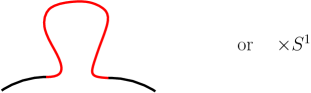
Figure 1. Corrugation in dimension one and two.

I should say that the theory of corrugation is still very lively for constructing concrete $C^{1}$ isometric embeddings (see V. Borrelli & al. [2]).

Figure 2. First corrugating step for an isometric embedding of the unit sphere into the ball of radius 1/2. By courtesy of the Hevea Project.

In the rest of Section 1, I would like to present Smale’s ideas, starting from the basics, and connect them with more recent ideas.

1.2. Immersions.

Given two smooth manifolds $X$ and $Y$ where the dimension of $X$ is not greater than the dimension of $Y$, a $C^{1}$-map $f:X\to Y$ is said to be an immersion if its differential $df$ is of maximal rank at every point of $X$. An immersion can have double points but no singular points like folds. An immersion with no double points is said to be an embedding. In that case, the image of $f$ is a submanifold under some properness condition, more precisely when $f$ is proper (in the topological sense) from $X$ to some open subset of $Y$ (Figure 3(A)).

The space of immersions from $X$ to $Y$, denoted by $Imm(X,Y)$, is an open set in $C^{1}(X,Y)$ if the space of $C^{1}$ maps is endowed with the so-called fine Whitney topology. When $X$ is compact, there is no concern: a sequence $\left(f_{n}\right)$ is convergent if and only if both sequences $\left(f_{n}(x)\right)$ and $\left(df_{n}(x)\right)$ converge uniformly. In what follows, we shall only consider immersions whose source is compact. In that case, the set of immersions is locally contractible.

Two immersions $f_{0},f_{1}:X\to Y$ are said to be regularly homotopic if they are joined by a path in $Imm(X,Y)$ or equivalently if $f_{0}$ and $f_{1}$ belong to the same path component of $Imm(X,Y)$.

Figure 3. (A) shows an embedding $(0,1)\to\mathbb{R}^{2}$ whose image is not a submanifold. (B) shows an immersion $\mathbb{S}^{1}\to\mathbb{R}^{2}$ which does not extend to an immersion of the 2-disc.

1.3. Whitney-Graustein Theorem

The immersions from the circle to the plane were classified by Whitney up to regular homotopy in the mid-thirties [43]. The classification reduces to the degree of the Gauss map

$$\begin{array}[]{rcl}G:\mathbb{S}^{1}&\to&\mathbb{S}^{1}\\ x&\mapsto&df_{x}(\partial_{\theta})/\|df_{x}(\partial_{\theta})\|\,,\end{array}$$

where $\partial_{\theta}$ stands for the unit tangent vector to the circle $\mathbb{S}^{1}:=\mathbb{R}/2\pi\mathbb{Z}$. The reason why this theorem is named Whitney-Graustein Theorem is given by Whitney himself in a footnote on page 279 of his article:

This theorem, together with a straightforward proof, was suggested to me by W. C. Graustein.

It is worth noticing that there is an interesting proof of the Whitney-Graustein Theorem given by S. Levy in [20, p. 33 - 37] following Thurston’s idea of corrugation.

It would be wrong to think that this classification ends the story of immersion of the circle to the plane. A much more difficult question is the following: Which immersions extend to an immersion of the disc to the plane? For such an immersion, how many extensions are there? An obvious necessary condition for a positive answer to the first question is that the degree of the Gauss map be equal to one. But that condition is not sufficient as Figure 3(B) shows. Actually, these questions have been solved by S. Blank in his unpublished thesis. Luckily, V. Poenaru reported on Blank’s thesis in a Bourbaki seminar [26]. The analogous questions for immersions of the $n$-sphere into $\mathbb{R}^{n+1}$ can be raised and remain essentially open.

1.4. The key proposition in Smale’s thesis.

Let $f_{0}$ denote the standard embedding of $S^{2}$ in $\mathbb{R}^{3}$. Choose an equator $E$ on $\mathbb{S}^{2}$, a base point $p\in E$ and two hemispheres respectively named the northern and the southern hemisphere $H_{N}$ and $H_{S}$. We consider the space of pointed immersions

$$Imm_{p}(\mathbb{S}^{2},\mathbb{R}^{3}):=\left\{f:\mathbb{S}^{2}\looparrowright\mathbb{R}^{3}\mid f(p)=f_{0}(p)\text{ and }df(p)=df_{0}(p)\right\}.$$

The spaces $Imm_{p}(H_{S},\mathbb{R}^{3})$ and $Imm_{p}(H_{N},\mathbb{R}^{3})$ are defined similarly. The space of immersions $H_{N}$ to $\mathbb{R}^{3}$ whose 1-jet $j^{1}\!f(x):=\bigl{(}f(x),df(x)\bigr{)}$ coincides with $j^{1}\!f_{0}(x)$ at every point $x\in E$ is denoted by $Imm_{E}(H_{N},\mathbb{R}^{3})$. Finally, $\widetilde{Imm}_{p}(E,\mathbb{R}^{3})$ stands for the space of immersions of $E$ to $\mathbb{R}^{3}$ enriched with a 2-framing along $E$ which is fixed at $p$ and whose generated plane field is tangent to $E$ and standard at $p$. The space of pointed immersions of the 2-disc to $\mathbb{R}^{3}$ is known to be contractible thanks to the Alexander’s contraction which reads in the present setting:

$$(x,t)\mapsto p+\frac{1}{t}[f\bigl{(}p+t(x-p)\bigr{)}-f(p)]$$

where $p$ lies in the boundary of $\mathbb{D}^{2}$ and $(x,t)\in\mathbb{D}^{2}\times(0,1]$. When $t$ goes to 0, the limit of the above expression, uniformly in $x$ in the 2-disc, is the affine map $x\mapsto p+df(p)(x-p)$.

Proposition.

1) The restriction map $Imm_{p}(\mathbb{S}^{2},\mathbb{R}^{3})\to Imm_{p}(H_{S},\mathbb{R}^{3})$ is a Serre fibration. Its fibre over $f_{0}$ is homeomorphic to $Imm_{E}(H_{N},\mathbb{R}^{3})$.

2) The 1-jet map along the equator, $Imm_{p}(H_{N},\mathbb{R}^{3})\to\widetilde{Imm}_{p}(E,\mathbb{R}^{3})$, is a Serre fibration. Its fibre over $(j^{1}\!f_{0})|_{E}$ is also homeomorphic to $Imm_{E}(H_{N},\mathbb{R}^{3})$.

A map $\rho:X\to Y$ between two arcwise connected spaces is said to be a Serre fibration when it has the parametric Covering Homotopy Property. More precisely, for every $\gamma:[0,1]\to Y$ and every $x_{0}$ in $X$ with $\rho(x_{0})=\gamma(0)$, there exists a lift $\tilde{\gamma}:[0,1]\to X$ of $\gamma$ starting from $x_{0}$; and similarly in families with parameters in the $n$-disc. In that case, there is a long exact sequence in homotopy.

It is worth noticing that similar statements for one-dimensional source were already present in Smale’s thesis (published in [27]).

The proof of the first item is sketched by a picture which shows the flexibility that the statement translates (Figure 4).

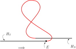
Figure 4. The southern hemisphere moves to the right. Only a northern collar of the equator in $H_{N}$ is deformed.

Corollary. We have $\pi_{0}\bigl{(}Imm_{p}(\mathbb{S}^{2},\mathbb{R}^{3})\bigr{)}=0$, that is, the space of pointed immersions of $\mathbb{S}^{2}\to\mathbb{R}^{3}$ is arcwise connected.

Proof. Since the base of the first Serre fibration is contractible, we have $\pi_{0}\bigl{(}Imm_{p}(\mathbb{S}^{2},\mathbb{R}^{3})\bigr{)}\cong\pi_{0}\bigl{(}Imm_{E}(H_{N},\mathbb{R}^{3})\bigr{)}$. By the second Serre fibration whose total space is contractible, we have $\pi_{0}\bigl{(}Imm_{E}(H_{N},\mathbb{R}^{3})\bigr{)}\cong\pi_{1}\bigl{(}\widetilde{Imm}_{p}(E,\mathbb{R}^{3})\bigr{)}$. Arguing similarly for the enriched immersions of $E$ whose equator is a 0-sphere, we get

$$\pi_{1}\bigl{(}\widetilde{Imm}_{p}(E,\mathbb{R}^{3})\bigr{)}\cong\pi_{2}\bigl{(}\widetilde{Imm}_{p}(S^{0},\mathbb{R}^{3})\bigr{)}\cong\pi_{2}(\{2\text{-frames in }\mathbb{R}^{3}\}\cong\pi_{2}(SO(3))=\pi_{2}(\mathbb{S}^{3})=0.$$

$\Box$

1.5. Concrete eversion of the sphere.

I do not intend to explain the history of this matter. I just give a list of references in chronological order and add a few comments: A. Phillips [22], G. Francis & B. Morin [6], Francis’ book [7] and finally the text and video by S. Levy [20].

The first idea, due to Arnold Shapiro, is to pass through Boy’s surface, here noted $\Sigma$, an immersion of the projective plane into the 3-space. Since the projective plane is non-orientable, a tubular neighborhood $T$ of $\Sigma$ is not a product. Therefore, $T$ is bounded by an immersed sphere $\tilde{\Sigma}$. It turns out that $\tilde{\Sigma}$ is endowed with the involution which consists of exchanging the two end points in each fibre of $T$. This is realized by the regular homotopy

$$\tilde{\Sigma}\times[0,1]\to T,\ (x,t)\mapsto x(1-2t)$$

where the product in the right hand side is associated to the affine structure of the fibre of $x$. If the two faces of $\tilde{\Sigma}$ are painted with different colors, this move has the effect of changing the color which faces Boy’s surface. It remains to connect the standard embedding of $S^{2}$ to Boy’s surface by a regular homotopy in order to get an eversion of the sphere.

Remembering a walk with Nicolaas Kuiper when he explained this construction to me, I had the feeling that he played himself a role in it. I did not know more until very recently, when Tony Phillips informed me about an article of Kuiper where his argument is written explicitly [17, p. 88]. The video [20] does not follow the same idea: it goes the way of Thurston’s corrugations and is not optimal in number of multiple points of multiplicity 3 or more.

1.6. Hirsch’s definitive statement.

The general statement in homotopy theory of immersions is due to M. Hirsch [15]. He considers any pair $(X,Y)$ of smooth manifolds. For simplicity, assume $X$ is connected. The main assumption is that $\dim X\leq\dim Y$, the equality being allowed only when $X$ is not closed (if $X$ is compact its boundary must be non-empty).

If $f:X\to Y$ is an immersion, we have a diagram

where $df$ is a fibre bundle map over $f$ (between the total spaces of the respective tangent bundles) which is fibrewise linear and injective.

Although the following terminology has been in use since Gromov’s thesis only, we are going to use it here. A formal immersion is a diagram

where $f$ is only assumed to be continuous and $F$ is a fibre bundle map which is fibrewise linear and injective. In the language of jet spaces, this is just a section of the 1-jet bundle $J^{1}(X,Y)$ over $X$ valued in the open set of 1-jets whose linear part is of maximal rank.

With this vocabulary at hand, Hirsch’s theorem states the following:

Theorem (Hirsch [15]). The space $Imm(X,Y)$ of immersions from $X$ to $Y$ has the same homotopy type as the space $Imm^{\rm formal}(X,Y)$ of formal immersions.

1.7. Phillips’ work on submersions.

When the dimension of $X$ is greater than the dimension of $Y$ it is natural to consider submersions, that is maps of maximal rank. When such maps exist they form a space that we denote by $Subm(X,Y)$. Using again the current terminology, a formal submersion is a section of the 1-jet bundle $J^{1}(X,Y)$ over $X$ valued in the open set of 1-jets whose linear part is of maximal rank. Phillips’ submersion theorem sounds similar to Hirsch’s immersion theorem with, nevertheless, a fundamental difference: the source needs to be an open manifold. Notice that the circle has no submersion to the line despite the existence of a formal submersion; a similar claim holds for any parallelizable manifold like a compact Lie group.

Theorem (Phillips [23]). If $X$ is an open manifold, $Subm(X,Y)$ and $Subm^{\rm formal}(X,Y)$ have the same homotopy type.

Since a foliation is locally defined by a submersion onto a local transversal, the next theorem can be viewed as an extension of the previous one. Let $\mathcal{F}$ be a smooth foliation of the manifold $Y$. Denote its normal bundle by $\nu(\mathcal{F})$; it is a vector bundle on $Y$ whose rank equals the codimension of $\mathcal{F}$. Denote by $\pi:TY\to\nu(\mathcal{F})$ the linear bundle morphism over $Id_{Y}$ whose kernel is the sub-bundle of $TY$ made of the tangent vectors to $Y$ which are tangent to the leaves of $\mathcal{F}$.

A smooth map $f:X\to Y$ is said to be transverse to $\mathcal{F}$ if the bundle morphism $\pi\circ df:TX\to\nu(\mathcal{F})$ over $f$ is fibrewise surjective. In that case, the preimage of $f^{-1}(\mathcal{F})$ is a foliation of the same codimension as $\mathcal{F}$ and its normal bundle is the pull-back $f^{*}\bigl{(}\nu(\mathcal{F})\bigr{)}$. We denote by $C^{\pitchfork\mathcal{F}}(X,Y)$ the set of smooth maps transverse to $\mathcal{F}$.

Given a bundle morphism $F:TX\to TY$ over $f:X\to Y$, the pair $(f,F)$ is said to be formally transverse to $\mathcal{F}$ if $\pi\circ F$ is fibrewise surjective. By abuse, one says also that $f$ is formally transverse to $\mathcal{F}$.

Theorem (Phillips [24]). The space $C^{\pitchfork\mathcal{F}}(X,Y)$ has the same homotopy type as the space of maps which are formally transverse to $\mathcal{F}$.

Remark. All previous theorems reduce the understanding of immersions, submersions or maps transverse to foliations from the homotopic point of view to the understanding of the corresponding formal problems. And the latter reduces to classical homotopy theory: the matter is to find sections to some maps and thus it reduces to well-known obstructions. This does not mean that the homotopy type of the formal spaces in question is computable. In general it is not, as the homotopy groups of the spheres are not completely computable.

The aim of Gromov’s approach which we are going to describe below is to consider all previous problems as particular cases of a general principle.

1.8. Differential relations after M. Gromov.

The main reference here is Gromov’s book [10]. A simplified approach is described in Y. Eliashberg & N. Mishachev’s book [5]; the new tool is their holonomic approximation Theorem which was first proved in [4].

The preface of [5] starts as follows:

A partial differential relation $\mathcal{R}$ is any condition imposed on the partial derivatives of an unknown function.

If the unknown function in question is a smooth map from $X$ to $Y$ – we limit ourselves to this case – a simple definition consists of saying that $\mathcal{R}$ is a subset in a jet space $J^{r}(X,Y)$ for some integer $r$. Recall that in coordinates an element of this jet space is just the data of a point $a\in X$, a point $b\in Y$ and a Taylor expansion of order $r$ at $a$ with constant term $b$.

The expression $h$-principle comes from the article of Gromov & Eliashberg [11]; they write:

The principle of weak homotopy equivalence for etc.

Later on, this expression is abbreviated to h-principle. With these authors we say that the parametric $h$-principle holds for $\mathcal{R}$ if the inclusion

$$sol\,\mathcal{R}\hookrightarrow sec\,\mathcal{R}$$

is a homotopy equivalence between

$$sol\,\mathcal{R}:=\{f:X\to Y\mid j^{r}\!f\text{ is valued in }\mathcal{R}\}$$

and

$$sec\,\mathcal{R}:=\{\text{sections of }J^{r}(X,Y)\text{ valued in }\mathcal{R}\}\,.$$

One can think of an element of $\sec\mathcal{R}$ as a formal solution of the problem posed by $\mathcal{R}$. A section valued in $\mathcal{R}$ which is of the form $j^{r}\!f$ is said to be holonomic or integrable. The integrablity is prescribed by the vanishing on the section in question of a list of 1-forms (called a Pfaff system) which are naturally defined on the manifold $J^{r}(X,Y)$. For instance, when $r=1$ and $Y=\mathbb{R}$, a section $s$ is integrable if and only if its image is Legendrian for the canonical contact form $\alpha$ which reads $dz-\sum p_{i}dq^{i}$ in canonical coordinates, that is, if $s^{*}\alpha=0$.

Theorem (Gromov [8]). If $\mathcal{R}$ is an open set in $J^{r}(X,Y)$ which is invariant under the natural right action of $\text{Diff}(X)$ and if $X$ is an open manifold (meaning that no connected component is closed), then the parametric $h$-principle holds true for $\mathcal{R}$.

The proof also goes through corrugations as said for Smale’s theorem. Of course, the corrugations are not developed in the range; there is no room for corrugating. They are developed in the domain. This is very clearly explained in Eliashberg-Mishachev’s book [5].

Remark. Another very important condition on a differential relation leads to an $h$-principle; it is when the relation is ample. In that case $X$ does not need to be an open manifold. Here, the $h$-principle follows from the famous convex integration technique which was invented by Gromov in [9] (see Gromov’s book [10]). A complete account on this is given in D. Spring’s book [32]. The end of Eliashberg-Mishachev’s book [5] focuses on convex integration applied to the $C^{1}$ isometric embedding problem (Nash-Kuiper); Borrelli & al. [2] converted their theoretical result into an algorithm richly illustrated by pictures of $C^{1}$ fractal objects, as the authors say. Despite the great interest of the subject, I do not intend to enter more deeply into it as it is less connected to the work of Thom than what follows.

Going back to the, say open, $h$-principle stated above, one sees that the previously mentioned results by Smale, Hirsch and Phillips are clearly covered by Gromov’s theorem. One could be disappointed that only the 1-jet space is involved. The simplest way to find new examples with differential relations of higher order consists of the following construction, which naturally appears in Thom’s singularity theory [35] as it is shown in the next subsection.

Consider a proper submanifold $\Sigma\subset J^{r-1}(X,Y)$ or a proper stratified set with nice singularities (for instance, with conical singularities in the sense of [18]); the important point is that transversality to any stratum $\Sigma_{i}\subset\Sigma$ implies transversality to all other strata in some neighbourhood of $\Sigma_{i}$ in $J^{r-1}(X,Y)$. Assume that $\Sigma$ is natural, that is invariant under the action of ${Dif\!f(X)}$. The transversality to $\Sigma$ is obviously a differential relation of order $r$. This differential relation which we denote by $\mathcal{R}_{\Sigma}$ is open and invariant under the action of ${Dif\!f(X)}$. Thus, if $X$ is open, Gromov’s theorem applies.

1.9. Examples from singularity theory.

For a first concrete example, take $\dim X=\dim Y=2$ and consider the stratified set $\Sigma$ of 1-jets of rank less that 2. It is made of two strata: one stratum is the set of jets of rank 1; it has codimension 1 and is denoted by $\Sigma^{1}$ in the so-called Thom-Boardman notation [1]. The other stratum is the rank zero one; it has codimension 4 in our setting. Their union is a stratified set with conical singularities which is natural and proper. Thus $\mathcal{R}_{\Sigma}$ satisfies the open $h$-principle if $X$ is open.

Figure 5. Local image of a cusp in a two-dimensional manifold.

The next example leads to an order 3 differential relation. One starts with the first example and looks at a 2-jet $\xi\in\mathcal{R}_{\Sigma}$; say it is based in $a\in X$. Since $\xi$ is transverse to $\Sigma$, it does not project to the zero 1-jet. Therefore, it determines the tangent space in $a$ to the fold locus $L\subset X$ where the rank of any germ of map $f$ realizing $\xi$ is exactly 1. In our setting, $L$ is one-dimensional. On the other hand, $\xi$ determines the kernel $K_{a}$ of the differential $df_{a}$. Thus, there is a natural stratification of $\mathcal{R}_{\Sigma}\subset J^{2}(X,Y)$: one stratum is $\Sigma^{1,0}$ which is made of 2-jets where $K_{a}$ is transverse to $T_{a}L$; the second one, denoted by $\Sigma^{1,1}$, is made of 2-jets where $K_{a}$ is tangent to $T_{a}L$. The stratum $\Sigma^{1,0}$ is an open set in $\mathcal{R}_{\Sigma}$ and $\Sigma^{1,1}$ has codimension 2 in $J^{2}(X,Y)$; it is a conical singularity of $\mathcal{R}_{\Sigma}$. Thus, if a 3-jet is transverse to $\mathcal{R}_{\Sigma}$, it is the jet of a germ having an isolated cusp from which emerge two branches of fold locus (see Figure 5).

1.10. Thom’s transversality theorem in jet spaces.

This was exactly the subject of Thom’s lecture at the 1956 Symposium in Mexico City that I mentioned at the very beginning of this piece. Incidently, this theorem will play a fundamental role in singularity theory, as the above discussion lets us foresee. The statement is the following:

Theorem (Thom [34]). Let $\Sigma$ be a submanifold in a $r$-jet bundle $E^{(r)}\to X$ over a manifold $X$. Then, generically, an integrable section of $E^{(r)}$ is transverse to $\Sigma$.

This theorem is remarkable in two ways:

1) The usual transversality statement tells us that any section of $E^{(r)}$ can be approximated by a section transverse to $\Sigma$. But, the integrability condition is a closed constraint and even if we started with an integrable section, the transverse approximation could be non-integrable.

2) The same proof, by inserting the given map in a large family of maps which is transverse to $\Sigma$ as a whole, works both for the usual transversality theorem and for the transversality theorem with constraints.

For many years I tried to understand whether the statements of Thom and Gromov were somehow related. For instance, does the $h$-principle hold for the relations $\mathcal{R}_{\Sigma}$ from subsection 1.9? The answer was shown to be no in general, in a note with Alain Chenciner [3]. Quoting from its abstract:

A section in the 2-jet space of Morse functions is not always homotopic to a holonomic section.

2. Integrability and related questions

2.1. Thom’s point of view in 1959.

The title of the lecture given by René Thom at the 1959 conference organized by the CNRS in Lille (France) is striking when compared with the terminology that would appear ten years later:

Remarques sur les problèmes comportant des inéquations différentielles globales

which I translate into: Remarks about problems involving global differential inequations.

The setting is the same as in Gromov’s theorem from Subsection 1.8 and, for consistency with what precedes, $\mathcal{R}$ still denotes an open set in the jet space $J^{r}(X,Y)$, except that now the openness of $X$ is not assumed. There are two chain complexes naturally associated with $\mathcal{R}$:

1. $C_{*}(\mathcal{R})$ is the complex of continuous singular simplices.

2. $C_{*}^{\rm int}(\mathcal{R})$ is the subcomplex generated by the differentiable simplices valued in $\mathcal{R}$ which are integrable (or holonomic) in the sense that each 1-form from the integrability Pfaff system vanishes on them.

Here, a $k$-simplex is a map from the standard $k$-simplex $\Delta^{k}\subset\mathbb{R}^{k+1}$ to $\mathcal{R}$. Thanks to the so-called small simplex Lemma, up to quasi-isomorphism, it is sufficient to consider holonomic smooth simplices of the form: $\sigma=j^{r}f\circ\underline{\sigma}$ where $\underline{\sigma}$ is a $k$-simplex of the base $X$ and $f$ is a smooth map defined near the image of $\underline{\sigma}$ with values in $Y$.

Theorem (Thom [37].) The inclusion $C_{*}^{\rm int}(\mathcal{R})\hookrightarrow C_{*}(\mathcal{R})$ induces an isomorphism in homology for $*<\dim X$ and an epimorphism for $*=\dim X$.

For instance, if $X$ is closed and $s:X\to\mathcal{R}$ is a section, then the cycle $s(X)$ (at least with $\mathbb{Z}/2\mathbb{Z}$ coefficients when $X$ is non-orientable) is homologous to a holonomic zig-zag, that is a cycle of the form $j^{r}f(X)$ where $f:X\to Y$ is multivalued.

2.2. What happened afterwards.

This article was actually only an announcement. The proof of the theorem was outlined in three pages, and was difficult to read although some ideas were visibly emerging; for instance the sawtooth, which is an antecedent to the jiggling intensively used by Thurston in the early seventies [39]. No complete proof ever appeared. Unfortunately, the report by Smale in the Math. Reviews [30] was somewhat discouraging for anyone who would have tried to complete Thom’s proof. Here is the final comment of this report:

{The author has said to the reviewer that, although he believes his proof to be valid for $r=1$, there seem to be further difficulties in case $r>1$.}

Nevertheless, David Spring has known for a few years that Thom’s statement holds true (see his note [33]). His unpublished proof is based on the holonomic approximation theorem of Eliashberg & Mishachev [4] when $*<\dim X$. In the remaining case, he also needs Poenaru’s foldings theorem [25]. I should say that the holonomic approximation theorem is in germ in Thom’s announcement; his horizontal sawtooth is closely related to the construction made in [4].

When reading Thom’s article for preparing the edition of his collected mathematical works [38], I was no more able to complete the proof in the way indicated by Thom, but I discovered a beautiful object in that article. I first translate the original few lines into English and then, in the next subsection, I shall state the lemma which I could extract from these lines.

[The proof] mainly relies on the construction of a deformation (homotopy operator) from the complex of all singular differentiable simplices to the integrable simplices. Such a deformation has to be « hereditary », that is, compatible with the restriction to faces. Moreover, as the problem is local in nature, it will be sufficient to construct this deformation for an open set in $J^{\prime r}(\mathbb{R}^{n},\mathbb{R}^{p})$.

… …

Let $b^{k}$ be a $k$-dimensional simplex, $b^{n}$ an $n$-dimensional simplex, $n\geq k$; let $b^{\prime k}$ be a subdivision of $b^{k}$ and $s$ a simplicial map from this subdivision $b^{\prime k}$ of $b^{k}$ to $b^{n}$. The finer the subdivision $b^{\prime}$ is, the more the map $s$ has a « strong gradient »  in the sense that the quotient $[s(x)-s(y)]/(x-y)$, for every pair of points $x,y\in B^{k}$ close enough, becomes larger and larger.

Here, the question is: why do such a subdivision and simplicial map exist?

2.3. Thom’s subdivision.

Here is the statement that I cooked up for translating the preceding lines into a more precise language.

Lemma. There exists a sequence $\left(K_{n},s_{n}\right)_{n}$, where $K_{n}$ is a linear subdivision of $\Delta^{n}$ and $s_{n}:K_{n}\to\Delta^{n}$ is a simplicial map such that:

1. (Non-degeneracy) for each $n$-simplex $\delta_{n}\subset K_{n}$, the restriction $s_{n}|_{\delta_{n}}$ is surjective;

2. (Heredity) for each $(n-1)$-face $F$ of $\Delta^{n}$ we have:

   $$\left\{\begin{array}[]{l}F\cap K_{n}\ \cong\ K_{n-1}\,,\\ s|_{F}\ \cong\ s_{n-1}\,.\end{array}\right.$$

Here, the symbol $\cong$ stands for simplicial isomorphism; if a numbering of the vertices of $\Delta^{n}$ is given there is a canonical simplicial isomorphism $F\cong\Delta^{n-1}$ for every facet $F$. The non-degeneracy somehow translates Thom’s strong gradient condition.

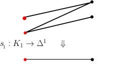
Figure 6. Thom subdivision in dimension 1 and its folding map.

The proof can be obtained by induction on $n$ in the way which is illustrated by passing from Figure 6 to Figure 7: put a small $n$-simplex $\delta^{n}$ upside down in the interior of $\Delta^{n}$ and join each vertex of $\delta^{n}$ to the facet of $\Delta^{n}$ lying in front of it which is already subdivided by induction hypothesis.

One can think of $s_{n}$ as a folding map from $\Delta^{n}$ onto itself. Due to the heredity property, we have:

• Any polyhedron can be folded onto itself.

• The folding can be iterated $r$ times:

  $$\begin{array}[]{lcl}K_{n}^{(r)}&=&\left(s_{n}^{(r-1)}\right)^{-1}(K_{n})\\ s_{n}^{(r)}&=&s_{n}\circ s_{n}^{(r-1)}\end{array}$$

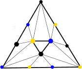
Figure 7. Thom subdivision in dimension two; $s_{2}$ is defined by the coloring.

Notice that the folding map of any order is endowed with an hereditary unfolding homotopy to Identity.

2.4. Jiggling formula

It is now easy to derive a natural jiggling formula, using the same terminology as Thurston’s in [39], but without any measure consideration.

Equip $X$ with a Riemannian metric. Let $DX\to X$ be a tangent disc bundle such that the exponential map $\text{exp}:DX\to X$ is a submersion. Choose a triangulation $T$ of $X$ finer than the open covering $\left\{\text{exp}_{x}(D_{x}X)\mid x\in X\right\}$. Fix an integer $r$. The $r$-th jiggling map is the section of the tangent bundle defined by

$$\begin{array}[]{c}j^{(r)}:X\to DX,\\ j^{(r)}(x)=\text{exp}_{x}^{-1}\bigl{(}s_{n}^{(r)}(x)\bigr{)}\,.\end{array}$$

This map is piecewise smooth. Moreover, the larger $r$ is, the more vertical the jiggling is.

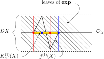
Figure 8. The jiggling map of order $r=1$. The vertical lines are fibres of $TX$.

As a consequence, for $r$ large enough, $j^{(r)}(X)$ is quasi-transverse to the tangent space to the exponential foliation $\mathcal{F}_{\rm exp}$, that is, for any simplex $\tau$ of the $r$-th Thom subdivision of $T$ the smooth image $j^{(r)}(\tau)$ shares no tangent vector with the tangent space to the leaves of $\mathcal{F}_{\rm exp}$. Actually, when $X$ is compact, this quasi-transversality holds with respect to any compact family of $n$-plane fields which are transverse to the fibres of $TX$, in place of $\mathcal{F}_{\rm exp}$.

2.5. Going back to immersions.

This is part of a joint work with Gaël Meigniez [19].

First, recall that one can reduce oneself to consider only immersions of codimension 0. Indeed, any formal immersion $(f,F)$ from $X$ to $Y$ ($\dim X<\dim Y$) has a normal bundle; it is the vector bundle over $X$ which is the cokernel $\nu(f,F)$ of the monomorphism $TX\to f^{*}TY$ through which $F$ factorizes. Thus, immersing $X$ to $Y$ is equivalent to immersing a disc bundle of $\nu(f,F)$ to $Y$ and the latter is a codimension 0 immersion.

In what follows, we assume that $X$ is compact with non-empty boundary and has the same dimension as $Y$. For free, a formal immersion $(f,F)$ from $X$ to $Y$ gives rise to a foliation $\mathcal{F}_{X}:=F^{-1}(\mathcal{F}_{{\rm exp}_{Y}})$ which foliates a neighbourhood of the zero section $O_{X}$ of $TX$. Indeed, since $F$ maps fibres to fibres surjectively, $F$ is transverse to the exponential foliation of $Y$ (defined near the zero section $O_{Y}$ of $TY$).

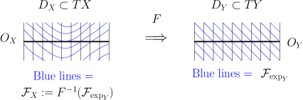
Figure 9. The left part shows a tangential Haefliger structure.

Such a (germ of) foliation like $\mathcal{F}_{X}$ is called a tangential Haefliger structure or a $\Gamma_{n}$-structure on $X$. We refer to [13] for more details on this important notion. Since there is no reason for $\mathcal{F}_{X}$ to be transverse to $O_{X}$, the trace of $\mathcal{F}_{X}$ on $X=O_{X}$ is in general a singular foliation.

Actually, those singularities are responsible for the flexibility associated with that concept: they allow for operations like induction (or pull-back) and homotopy (or concordance). Let us emphasize that a $\Gamma_{n}$-structure is mainly a $\check{\rm C}$ech cocycle of degree one valued in the groupoid of germs of diffeomorphisms of $\mathbb{R}^{n}$. This allows one to induce such a structure on a polyhedron or a CW-complex. A concordance between two $\Gamma_{n}$-structures $\xi_{0},\xi_{1}$ on $X$ is just a $\Gamma_{n}$-structure on $X\times[0,1]$ which induces $\xi_{i}$ on $X\times\{i\},\,i=0,1$. There is a classifying space $B\Gamma_{n}$ in the following sense: the $\Gamma_{n}$-structures on $X$, up to concordance, are in 1-to-1 correspondance with the homotopy classes $[X,B\Gamma_{n}]$, as for vector bundles.

In our setting, the Haefliger structure in question is enriched with a transverse geometric structure invariant under holonomy: each transversal to $\mathcal{F}_{X}$ is endowed with a submersion to $Y$ which is preserved when moving the transversal by isotopy along the leaves (this point being obvious since the leaves in question are contained in the inverse images of points in $Y$); such a $\Gamma_{n}$-structure will be named a $\Gamma_{n}^{Y}$-structure. In particular, if $O_{X}$ were transverse to $\mathcal{F}_{X}$, then $X$ would be endowed with a submersion to $Y$, that is an immersion to $Y$ as $\dim X=\dim Y$. Therefore, the aim is to remove the singularities of the $\Gamma_{n}^{Y}$-structure, that is, to find a regularizing concordance of $\Gamma_{n}^{Y}$-structures from $\mathcal{F}_{X}$ to a $\Gamma_{n}^{Y}$-structure whose underlying foliation is transverse to the zero section.

In the next subsection we give a brief review of the regularization problem, and in the last subsection a sketch of the regularization is given in our setting of immersions in codimension 0 of compact manifolds with non-empty boundary and no closed connected components.

2.6. About the regularization of $\Gamma$-structures.

Let $\xi$ be a $\Gamma_{q}$-structure on an $n$-dimensional manifold $X$. In general, the underlying foliation $\mathcal{F}(\xi)$ is supported in a neighbourhood of the zero-section in a vector bundle $\nu(\xi)$ of rank $q$, called the normal bundle to $\xi$. This normal bundle remains unchanged along a concordance. If $\xi$ is regular, that is, if $\mathcal{F}(\xi)$ is transverse to the 0-section of $\nu(\xi)$, then the trace of $\mathcal{F}(\xi)$ on $X$ is a genuine foliation whose normal bundle is canonically isomorphic to $\nu(\xi)$. Therefore, a necessary condition to be regularizable is that $\nu(\xi)$ embed into the tangent bundle $TX$; in particular, $q\leq n$.

André Haefliger was the first to prove that any $\Gamma_{q}$-structure on an open manifold $X$ whose normal bundle embeds into $TX$ is regularizable [12] (or [13, p. 148]). That follows from two things: first, the classifying property of the classifying space $B\Gamma_{q}$: the latter is equipped with a universal $\Gamma_{q}$-structure which induces by pull-back all others; second, the Phillips transversality theorem to a foliation [24] (see the statement in Subsection 1.7). Today, this regularization theorem is frequently referred to as the Gromov-Haefliger-Phillips theorem.

The next step was done by W. Thurston [39]. If $q>1$, even when $X$ is closed, any $\Gamma_{q}$-structure satisfying the necessary condition is regularizable. The case $q=n$ is the toy case. The only technique is the famous jiggling lemma whose proof is quite tricky in terms of measure theory, despite its author considered it as obvious. Exactly at this point, our jiggling based on the Thom subdivision is much simpler; moreover, it works in families.

The final step is the codimension-one case for closed manifolds, a piece of work indeed. Generally it is known in the following form:

Theorem (Thurston [40]). Every hyperplane field is homotopic to the field tangent to some codimension-one foliation.

Actually, the main part of that result is a regularization theorem for $\Gamma_{1}$-structures. In addition to the jiggling technique, there are many subtle points (simplicity of the group of diffeomorphisms, intricate constructions, etc.).

2.7. Regularization of transversely geometric $\Gamma_{n}$-structures.

In Subsection 2.5 we reduced the problem of immersion to a problem of regularization of some $\Gamma_{n}^{Y}$-structure $\xi$ on $X$ associated with the given formal immersion and shown in Figure 9. The exponent $Y$ reminds us that we are considering a $\Gamma_{n}$-structure endowed with some transverse geometry which here consists of being endowed with a submersion to $Y$. The scheme shown in Figure 10, and on which I am going to comment, summarizes an ordinary regularization (which would work even if $X$ were closed). It will appear in the end that this regularization is easily enriched with a transverse geometric structure when $X$ is open. It is worth noticing that the problem is the same whatever the transverse geometry is. In place of submersion to $Y$ one could have a symplectic or contact structure, a complex structure or a codimension-one foliated structure etc.. For any geometry, the regularization is the same.

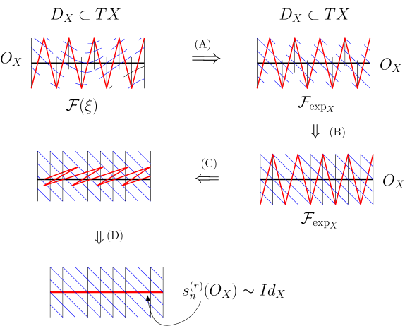
Figure 10. The scheme of the regularization in four steps.

First, the jiggling is chosen, meaning that the order of the Thom subdivision $r$ is fixed once and for all. This $r$ is chosen so that $j^{(r)}(X)$ is quasi-transverse to the following codimension-$n$ foliations or plane fields:

• the foliation $\mathcal{F}(\xi)$ underlying the given $\Gamma_{n}$-structure $\xi$ (this foliation was denoted by $\mathcal{F}_{X}$ in the particular case of Figure 9);

• the exponential foliation $\mathcal{F}_{\text{exp}_{X}}$;

• every $n$-plane field which is a barycentric combination of the two previous ones.

The homotopy from the zero-section to $j^{(r)}(X)$ gives rise to an obvious concordance which is not mentioned in the scheme of Figure 10.

Step (A) is exactly Thurston’s concordance in [39]. By using the above-mentioned barycentric combination, some generic $(n+1)$-plane field $\Pi$ is chosen on $TX\times[0,1]$ quasi-transverse to $j^{(r)}(X)\times[0,1]$. Since the trace of $\Pi$ on each simplex of the jiggling is 0- or 1-dimensional, such a trace is integrable. Thus, a $C^{0}$ approximation of $\Pi$ is integrable in a neighbourhood of $j^{(r)}(X)\times[0,1]$. This gives the concordance (A) and explains the reason why some part of the tube $D_{X}$ has been deleted from the initially foliated domain.

Step (B) is just the inclusion using the fact that the exponential foliation exists on the whole tube. Step (C) uses the interpolation $\text{exp}^{t}$, $t\in[0,1]$, from $Id_{DX}$ to $\text{exp}:DX\to X$ given by:

$$(x,u)\longmapsto\left(\text{exp}_{x}(tu),\left(D_{(x,tu)}\text{exp}_{x}(tu)\right)(1-t)u\right).$$

It allows one to slide $j^{(r)}(X)$ along the leaves of the exponential foliation keeping the quasi-transversality to each simplex. Observe that the vertical homothety does not have such a property. When $t=1$, we finish with the folding map $s_{n}^{(r)}(X)\to X$. Step (D) is just the unfolding of $s_{n}^{(r)}$, that is, its hereditary homotopy to $Id_{X}$. Again, at each time of the homotopy, the image polyhedron (contained in the zero-section) is quasi-transverse to the exponential foliation. This finishes the regularization of $\xi$ as a $\Gamma_{n}$-structure. In general, it is not possible to extend the transverse geometry to the concordance. But, this is possible when $X$ is an open manifold as we are going to explain.

If $X$ is an $n$-dimensional manifold without closed connected component, endowed with a triangulation $T$, there exists a spine, that is, a subcomplex $K$ of dimension $n-1$ such that, for any neighbourhood $N(K)$, there is an isotopy of embeddings $\varphi_{t}:X\to X$ whose time-one maps $X$ into $N(K)$ (see for instance [5, p. 40-41]).

Restricting ourselves to $K\subset X$, let us consider the concordance $(W,\mathcal{F}_{W})$ of $\Gamma_{n}$-structures obtained by concatenation and time reparametrization of the four concordances described right above from $j^{(r)}(K)$ to $K\subset O_{X}$. Here, $W\subset TX\times[0,1]$ is piecewise linear homeomorphic to $X\times[0,1]$; and $\mathcal{F}_{W}$ is a codimension-$n$ foliation defined near $W$ and transverse to the fibres of $TX\times[0,1]\to X\times[0,1]$ which induces $\mathcal{F}(\xi)$ over $t=0$ and $\mathcal{F}_{{\rm exp}_{X}}$ over $t=1$. Moreover, $\mathcal{F}_{W}$ is quasi-transverse to every simplex of $W$. Therefore, since $W$ is $n$-dimensional, every leaf meets each simplex of $W$ in one point at most.

By construction, $W$ collapses onto its initial face $W_{0}:=j^{(r)}(K)$. We recall that a simplicial complex $W$ collapses to $W_{0}$ if there is a sequence of elementary collapses $W_{q+1}\searrow W_{q}$ starting with $W$ and ending with $W_{0}$. An elementary collapse means that $W_{q+1}$ is the union of $W_{q}$ and a simplex $\sigma_{q}$ so that $\sigma_{q}\cap W_{q}$ consists of the boundary of $\sigma_{q}$ with an open facet removed. The elementary collapse $W_{q+1}\searrow W_{q}$ gives rise to an elementary isotopy $\chi_{q}^{t}$ pushing $W_{q+1}$ into itself, keeping $W_{q}$ fixed, and ending with $\chi_{q}^{1}(W_{q+1})$ as close to $W_{q}$ as we want. Due to the quasi-transversality to $\mathcal{F}_{W}$ this isotopy extends to a neighbourhood of $\sigma_{q}$ as a foliated isotopy $\tilde{\chi}_{t}$, meaning that leaf is mapped to leaf at each time.

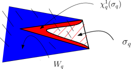
Figure 11. A few leaves of $\mathcal{F}_{W}$ are drawn in black. The simplex $\sigma_{q}$ is the union of the red full part and the red dashed part.

By induction on $q$, assume that the transverse geometric structure already exists on the foliation $\mathcal{F}_{W}|_{W_{q}}$. Then, by pulling back through $\tilde{\chi}_{q}^{1}$, this structure extends to the foliation $\mathcal{F}_{W}|_{W_{q+1}}$. Finally, the whole foliation $\mathcal{F}_{W}$ is enriched with the considered geometry, for instance a submersion to $Y$. And hence, $N(K)$ is endowed with a submersion to $Y$.

2.8. Sphere eversion again.

The main advantage of this proof based on the Thom subdivision and its associated jiggling is that it works in families (or with parameters). It is sufficient to choose the order $r$ large enough so that a common jiggling is convenient for each member of the family.

For instance, if $f_{0}$ denotes the inclusion $S^{2}\hookrightarrow\mathbb{R}^{3}$ and $f_{1}:=-f_{0}$, these two immersions are formally homotopic by:

$$(f_{t},F_{t}):\ (x,\vec{u})\mapsto\left(tf_{1}(x)+(1-t)f_{0}(x),R_{Ox}^{\pi t}(\vec{u})\right).$$

Here, $t\in[0,1]$ is the parameter of the homotopy, $x$ is a point in $\mathbb{S}^{2}$ and $\vec{u}$ is a vector in $\mathop{\mathbb{R}}\limits^{\to}\,\!\!{}^{3}$, the vector space underlying the affine space $\mathbb{R}^{3}$, tangent to $S^{2}$ at $x$; and $R_{Ox}^{\pi t}$ stands for the Euclidean rotation of angle $\pi t$ in $\mathop{\mathbb{R}}\limits^{\to}\,\!\!{}^{3}$ around the oriented axis directed by $\vec{x}$. When $t=1$, we have indeed $F_{1}(x,-)=d_{x}f_{1}(-)$, the differential of $f_{1}$ at $x$.

By thickening, we have a one-parameter family $F_{t}$ of formal submersions of $S^{2}\times(-\varepsilon,+\varepsilon)$ to $\mathbb{R}^{3}$. Thus, we have a one-parameter family of $\Gamma_{3}$-structures equipped with a transverse geometry (the local submersion to $\mathbb{R}^{3}$). The regularization by the Thom jiggling method – one jiggling for all foliations $F_{t}^{-1}(\mathcal{F}{{\rm exp}_{\mathbb{R}^{3}}}$) – gives rise to a one-parameter family of submersions $S^{2}\times(-\varepsilon,+\varepsilon)\to\mathbb{R}^{3}$ joining the respective thickenings of $f_{0}$ and $f_{1}$. The restriction to $S^{2}\times\{0\}$ is a regular homotopy from $f_{0}$ to $f_{1}$. This is the desired sphere eversion.

Here is a final remark. Since $f_{0}$ and $f_{1}$ have the same image, we get that the space of non-oriented immersed 2-spheres in the 3-space is not simply connected. Maybe, those who were skeptical about the sphere eversion thought that the orientation should be preserved. Of course, if an orientation is chosen on the initial sphere, it propagates along any regular homotopy. But, as the image is changing it does not prevent us from a change of orientation when the final image is the same as the original one. This is a phenomenon of monodromy well-known for detecting non-simply-connectedness.

Acknowledgements. I am indebted to Tony Phillips who provided important information to me about the time of the sphere eversion. I thank Paolo Ghiggini for helpful advice. I also thank Peter Landweber who read very carefully the first posted version and sent good remarks to me.

References

- [1] Boardman J.M., Singularities of differentiable maps, Publ. Math. IHES vol. 33, (1967), 21-57.
- [2] Borrelli V., Jabrane S., Lazarus F., Thibert B., Isometric embedding of the square flat torus in ambient space, Ensaios Mat. 24, Soc. Bras. Mat., 2013.
- [3] Chenciner A. & Laudenbach F., Morse 2-jet space and -principle, Bull. Braz. Math. Soc. 40(4) (2009), 455-463.
- [4] Eliashberg Y. & Mishachev N., Holonomic approximation and Gromov’s h-principle, p. 271 - 285 vol. I in: Essays on geometry and related topics, Monogr. Enseign. Math. 38, Geneva, 2001.
- [5] ———– , Introduction to the -principle, Graduate Studies in Math. 48, Amer. Math. Soc., 2002.
- [6] Francis G. & Morin B., Arnold Shapiro’s eversion of the sphere, Math. Intelligencer 2 (1979), 200-203.
- [7] Francis G., A Topological Picturebook, Springer, 1987.
- [8] Gromov M., Stable mappings of foliations, Izv. Akad. Nauk SSSR Ser. Mat. 33 (1969), 707-734; English translation, Math. USSR-Izv. 3 (1969), 671-694. MR 41 #7708.
- [9] ———– , Convex integration of differential relations I, Izv. Akad. Nauk SSSR Ser. Mat. 37 (1973), 329-343; English translation, Math. USSR-Izv. 7 (1973), 329-343.
- [10] ———– , Partial Differential Relations, Ergeb. Math. vol. 9, Springer, 1986.
- [11] Gromov M. & Eliashberg Y., Removal of singularities of smooth mappings, Izv. Akad. Nauk SSSR Ser. Mat. 35 (1971), 600-627; English translation: Math. USSR-Izv. 5 (1971), 615-639.
- [12] Haefliger A., Feuilletages sur les variétés ouvertes, Topology 9 (1970), 183- 194.
- [13] ——– , Homotopy and integrability, 133-175 in: Manifolds - Amsterdam 1970, Lect. Notes in Math. 197, Springer, 1971.
- [14] Herlihy M. & N. Shavit, A simple constructive computability theorem for wait free computation, Proceedings of the Twenty-sixth Annual AMC Symposium on Theory of Computing (STOC 94), pp. 243-252, AMC, New York, ISBN:0-89791-663-8.
- [15] Hirsch M. W., Immersions of manifolds, Trans. Amer. Math. Soc. 93 (1959), 242-276.
- [16] ————– , The work of Stephen Smale in differential topology, p. 29-52 in: [31, vol. 1].
- [17] Kuiper N., Convex immersions in , Non-orientable closed surfaces in with minimal total absolute Gauss-curvature, Comment. Math. Helv. 35 (1961), 85-92.
- [18] Laudenbach F., On the Thom-Smale complex, Appendix to: Bismut J.-M. & Zhang W., An extension of a Theorem by Cheeger and Müller, Astérisque 205 (1992), 219-233.
- [19] ——— & Meigniez G., Haefliger structures and symplectic/contact structures, J. École polytechnique 3 (2016), 1-29.
- [20] Levy S., Making waves, A guide to the ideas behind Outside In, (text and video), AK Peters, Wellesley (MA), 1995.
- [21] Palais R., Homotopy theory of infinite dimensional manifolds, Topology 5 (1966), 1-16.
- [22] Phillips A., Turning a surface inside out, Scientific American 214 (May 1966), 112-120.
- [23] ——– , Submersions of open manifolds, Topology 6 (1967), 171-206. MR 34 #8420
- [24] ——– , Smooth maps transverse to a foliation, Bull. Amer. Math. Soc. 76 n (1970), 792-797. MR 41 #7711
- [25] Poenaru V., On regular homotopy in codimension , Ann. of Math. 83 (1966), 257-265.
- [26] ———— , Extension des immersions en codimension 1 (d’après S. Blank), exposé n∘ 342, p. 473-505 in: Séminaire N. Bourbaki, vol. 10, 1966-1968, Soc. Math. de France, 1995; (online) Eudml.
- [27] Smale S., Regular curves on Riemannian manifolds, Trans. Amer. Math. Soc. 87 (1958), 492-512.
- [28] ———– , A classification of immersions of the 2-sphere, Abstract 380t, Bulletin Amer. Math. Soc. 63 (3) (1957), p. 196.
- [29] ——— , A classification of immersions of the two-sphere, Trans. Amer. Math. Soc. 90 (1959), 281-290.
- [30] ——— , Review of [37], MR0121807, Amer. Math. Soc. (1961).
- [31] ——— , Collected work of Stephen Smale, Ed. F. Cucker & R. Wong , World Scientific Publishing, 2000.
- [32] Spring D., Convex Integration Theory, Monographs in Math. 92, Birkhäuser, 1998.
- [33] ———— , Comments (to [37]), p. 558-560 in: [38, vol. 1].
- [34] Thom R., Un lemme sur les applications différentiables, Boletin de la Sociedad Matemática Mexicana 1 (1956), 59-71.
- [35] ——— , Les singularités des applications différentiables, Ann. Institut Fourier 6, (1955-1956), 43-87.
- [36] ——— , La classification des immersions (d’après S. Smale), exposé n∘157, p. 279-289 in: Séminaire N. Bourbaki, vol. 4, 1956-1958, Soc. Math. de France, 1995; (online) Eudml.
- [37] ——– , Remarques sur les problèmes comportant des inéquations différentielles globales, Bull. Soc. Math. France 87 (1959), 455-461; MR 22 #1253; or p. 549-555 in [38].
- [38] ——– , Œuvres mathématiques, volume 1, Documents Mathématiques 15, Soc. Math. de France, 2017.
- [39] Thurston W., The theory of foliations of codimension greater than one, Comment. Math. Helv. 49 (1974), 214-231.
- [40] ———– , Existence of codimension-one foliations, Annals of Math. 104 (1976), 249-268.
- [41] ———– , Making waves: The theory of corrugations in: [20].
- [42] Veblen O. & Whitehead J. H. C., A set of axioms for differential geometry, Proceedings of the National Academy of Sciences 17, 10 (1931), 551-561.
- [43] Whitney H., On regular closed curves in the plane, Compositio Math. vol. 4 (1937), 276-284.
- [44] ————— , Geometric Integration Theory, Princeton Univ. Press, 1957.