Parametrized-4.5PN TaylorF2 approximant(s) and tail effects to quartic nonlinear order from the effective one body formalism.

Abstract

By post-Newtonian (PN) expanding the well-known, factorized and resummed, effective-one-body energy flux for circularized binaries we show that: (i) because of the presence of the resummed tail factor, the 4.5PN-accurate tails-of-tails-of-tails contribution to the energy flux recently computed by Marchand et al. [Class. Q. Grav. 33 (2016) 244003] is actually contained in the resummed expression; this is also the case of the the next-to-leading-order tail-induced spin-orbit term of Marsat et al. [Class. Q. Grav. 31 (2014) 025023]; (ii) in performing this expansion, we also obtain, for the first time, the explicit 3.5PN leading-order tail-induced spin-spin flux term; (iii) pushing the PN expansion of the (nonspinning) EOB flux up to 5.5PN order, we compute 4PN, 5PN and 5.5PN contributions to the energy flux, though in a form that explicitly depends on, currently unknown, 4PN and 5PN non-test-mass corrections to the factorized waveform amplitudes. Within this (parametrized) 4.5PN accuracy, we calculate the Taylor F2 approximant. Focusing for simplicity on the nonspinning case and using the numerical-relativity calibrated IMRPhenomD waveform model as benchmark, we demonstrate that it is possible to reproduce the derivative of the IMRPhenomD phase (say up to the frequency of the Schwarzschild last-stable-orbit) by flexing only a 4PN “effective” waveform amplitude parameter. A preliminary analysis also illustrates that similar results can be obtained for the spin-aligned case provided only the leading-order spin-orbit and spin-spin terms are kept. Our findings suggest that this kind of, EOB-derived, (parametrized), higher-order, PN approximants may serve as promising tools to construct Inspiral-Merger-Ringdown phenomenological models or even to replace the standardly used 3.5PN-accurate TaylorF2 approximant in searches of small-mass binaries.

I Introduction

Effective-one-body (EOB) Buonanno and Damour (1999, 2000); Damour (2001); Buonanno et al. (2006) waveforms informed by numerical relativity (NR) simulations Damour et al. (2002); Damour and Nagar (2007); Damour et al. (2008) have played a central role in the detection, subsequent parameter-estimation Abbott et al. (2016a) analyses and GR tests Abbott et al. (2016b) of the gravitational-wave (GW) observations GW150914 Abbott et al. (2016c) and GW151226 Abbott et al. (2016d, e) announced in 2015. EOB waveforms have also been employed to build frequency-domain, phenomenological models for the inspiral, merger and ringdown stages of the binary black hole (BBH) coalescence Khan et al. (2016). Those models were also used to infer the properties Abbott et al. (2016a) and carry out tests Abbott et al. (2016b) of GR with GW150914 and GW151226. Despite the success of the EOBNR enterprise, one has to remember that EOB waveforms do not currently cover the full range of total masses to which the LIGO/Virgo detectors might be sensitive. In fact, for small-mass binaries, with $M<4M_{\odot}$ where $M=m_{1}+m_{2}$ is the total mass of the system, searches are done using post-Newtonian (PN) approximants, notably the Taylor F2 frequency domain one constructed using the stationary phase approximation (SPA, see e.g. Ref. Buonanno et al. (2009) and references therein). This approximant is computed at 3.5PN total accuracy, involving also spin-orbit and spin-spin terms. In addition, the 3.5PN-accurate Taylor F2 approximant is also used within the construction of the inspiral part of Inspiral-Merger-Ringdown phenomenological waveforms models, like IMRPhenomD Khan et al. (2016): its phasing is modified by the addition of effective parameters that are fitted to EOB-NR hybrid waveforms. By contrast, EOB models incorporate 4PN-accurate orbital information Bini and Damour (2013); Damour et al. (2016, 2015, 2014); Bernard et al. (2016, 2017), some test-particle information up to 5PN in the waveform Damour and Nagar (2009), the spin-spin interaction is incorporated in a special resummed form Damour and Nagar (2014); Balmelli and Damour (2015) as well as tail effects Damour and Nagar (2007); Damour et al. (2009). In practice, since the EOB model actually employs analytical information that is at higher PN-accuracy than the 3.5PN (and in fact for some parts, like the tail factor, it is using infinite PN accuracy), and since the PN-expansion is contained within the EOB model, it is actually possible to derive PN approximants beyond the 3.5PN order, though with some parameters that account for those specific terms (that depend on the symmetric mass ratio only $\nu\equiv\mu/M=m_{1}m_{2}/(m_{1}+m_{2})^{2}$) that are not fully known yet in PN theory). These additional parameters, that are inspired by EOB knowledge, could be then be informed by comparison with long-inspiral EOB or NR waveforms. A flavor of this idea was given already in Ref. Damour et al. (2012), that computed the tidal part of the Fourier domain phase at 2.5PN accuracy, including tail terms, but with the explicit dependence on a (still) unknown 2PN tidal waveform term. Once these, parametrized (EOB-NR informed), new approximants are obtained, one may then ask whether they are any better than the plain 3.5PN one during the inspiral and, in particular, whether they might be reliable (e.g., against NR calibrated NR waveforms) also for searches with larger values of $M$. If it were the case, one could exploit improved, computationally inexpensive, PN approximants beyond the mass range considered up to now.

The main purpose of this paper is to derive, from EOB first principles, families of parametrized, higher-PN, approximant, in order to give a general framework in which this problem can be properly addressed. In practice, we present here two results. On the one hand, starting from the well-known, factorized and resummed, EOB energy flux and PN-expanding it up to 5.5PN order (for the nonspinning case), we recover several high-order tail terms (notably the 4.5PN one) in the energy flux of circularized binaries recently computed using the Multipolar-Post-Minkowskian (MPM) formalism Marchand et al. (2016); Marsat et al. (2014) In doing so, we also obtain, for the first time at best of our knowledge, the leading-order spin-spin tail-induced term in the energy flux, finding it perfectly consistent with the test-mass results. Then, focusing on the nonspinning case for simplicity, we deliver a new 4.5PN-accurate TaylorF2 approximant in parametrized form, where the (two) parameters account for yet uncalculated 4PN-accurate waveform information, and we briefly investigate its flexibility and properties by comparison with the IMRPhenomD phenomenological model of Ref. Khan et al. (2016).

The paper is organized as follows: In Sec. II we obtain this parametrized 5.5PN accurate (nonspinning) flux and notably the 4.5PN tail term of Ref. Marchand et al. (2016). We note, in passing, that this term is part of the EOB resummed formalism from 2008 Damour et al. (2009); Damour and Nagar (2009), though it was never written down explicitly. Section III focuses on tail-induced spin terms: the NLO spin-orbit-induced tail term of Ref. Marsat et al. (2014) is obtained explicitly and, in addition, we similarly write down the LO spin-spin tail-induced term; Section IV illustrates the parametrized 4.5PN TaylorF2 approximant and gives an extensive comparison with the IMRPhenomD model. A very preliminary investigation of the spinning case is also discussed. Finally, we summarize our findings in Sec. V. If not otherwise specified, we use units where $c=G=1$.

II Parametrized 5.5PN, nonspinning flux from the effective-one-body framework

The aim of this Section is to compute the energy flux for nonspinning binaries at 5.5PN order by Taylor expanding the corresponding, factorized and resummed, EOB energy flux Damour et al. (2009); Damour and Nagar (2009). Evidently, since the $\nu$-dependent information is incomplete both at 4PN and at 5PN order, the final result will be obtained in parametrized form, with specific parameters, that have clear mining within the EOB framework, accounting for this yet uncalculated, $\nu$-dependent, information. In performing this calculation, we will also obtain as a bonus, and independently, the 4.5PN tail term recently computed by Marchand et al. Marchand et al. (2016) using the MPM formalism.

Going into detail, let us first recall the structure of the EOB energy flux. It is written as a sum of multipoles as

$${\cal F}=\sum_{\ell=2}^{\infty}\sum_{\ell=-m}^{m}F^{\rm Newt}_{{\ell m}}\hat{F}_{{\ell m}}$$ (1)

where $F^{\rm Newt}_{\ell m}$ is the usual Newtonian (leading-order) contribution and $\hat{F}_{\ell m}$ is the post-Newtonian correction. Within the EOB framework, this latter is written in a special factorized and resummed form as Damour et al. (2009)

$$\hat{F}_{\ell m}=\left(S^{(\epsilon)}_{\rm eff}\right)^{2}|T_{\ell m}|^{2}(\rho_{\ell m})^{2\ell},$$ (2)

where $S^{(\epsilon)}_{\rm eff}$ is the effective source, that is the effective EOB energy $\hat{E}_{\rm eff}(x)\equiv E_{\rm eff}/\mu$ when $\epsilon=0$ ($\ell+m$=even) or the Newton-normalized orbital angular momentum when $\epsilon=1$ ($\ell+m$=odd). The (complex) tail factor $T_{\ell m}$ resums an infinite number of leading order logarithms. See Refs. Damour et al. (2009); Faye et al. (2015). Starting from Eqs. (1)-(2), by means of a straightforward calculation one can show that the 4.5PN term of Marchand et al. (2016) is exactly contained in these expressions. The square modulus of the tail factor reads

$$|T_{\ell m}(x)|^{2}=\dfrac{4\pi Emx^{3/2}\prod_{s=1}^{\ell}\left(s^{2}+(2Emx^{3/2}\right)^{2}}{(\ell!)^{2}\left(1-e^{-4\pi mE}\right)},$$ (3)

where $x=(GM\Omega/c^{3})^{2/3}$ and $E$ is the energy of the system. In a dynamical EOB evolution, $E$ is given by the EOB Hamiltonian evaluated along the dynamics (and in fact the orbital frequency parameter $x$ is actually replaced by the orbital velocity $v_{\varphi}^{2}$). Here, $E$ is given by its PN expansion along circular orbit. Dropping for the moment the spin-dependence, that will be discussed in the next section, to obtain the PN-expanded energy flux at 5PN we need to retain $E$ and $S^{(\epsilon)}_{\rm eff}$ along circular orbits up to 4PN order. The PN expansions of $E(x)$ along circular orbits reads (see Refs. Damour et al. (2014, 2015, 2016); Bernard et al. (2017))

$$E(x)=1-\dfrac{\nu}{2}x+\left(\frac{\nu^{2}}{24}+\frac{3\nu}{8}\right)x^{2}+\left(\frac{\nu^{3}}{48}-\frac{19\nu^{2}}{16}+\frac{27\nu}{16}\right)x^{3}$$

$$+\left[\frac{35\nu^{4}}{10368}+\frac{155\nu^{3}}{192}+\left(\frac{205\pi^{2}}{192}-\frac{34445}{1152}\right)\nu^{2}+\frac{675\nu}{128}\right]x^{4}$$

$$+\Bigg{[}-\frac{77\nu^{5}}{62208}-\frac{301\nu^{4}}{3456}+\left(\frac{498449}{6912}-\frac{3157\pi^{2}}{1152}\right)\nu^{3}$$ (4)

$$+\left(\frac{123671}{11520}-\frac{9037\pi^{2}}{3072}-\frac{448}{15}{\rm eulerlog}_{2}(x)\right)\nu^{2}-\frac{3969}{256}\nu\Bigg{]}x^{5},$$

where ${\rm eulerlog}_{m}(x)\equiv\gamma_{\rm E}+\log(2)+\dfrac{1}{2}\log(x)+\log(m)$ and $\gamma_{E}$ is the Euler constant.

The effective EOB energy along circular orbits $\hat{E}_{\rm eff}(x)$ is obtained from the EOB mapping between the real and effective Hamiltonians Buonanno and Damour (1999) $E(x)=M\sqrt{1+2\nu(\hat{E}_{\rm eff}-1)}$ and reads

$$\hat{E}_{\rm eff}(x)=1-\frac{x}{2}+\left(\frac{\nu}{6}+\frac{3}{8}\right)x^{2}+\left(\frac{27}{16}-\frac{11\nu}{8}\right)x^{3}$$

$$+\left(-\frac{\nu^{3}}{162}+\frac{17\nu^{2}}{12}+\left(\frac{205\pi^{2}}{192}-\frac{4417}{144}\right)\nu+\frac{675}{128}\right)x^{4}$$

$$+\Bigg{[}-\frac{\nu^{4}}{486}-\frac{115\nu^{3}}{216}+\left(\frac{74899}{864}-\frac{943\pi^{2}}{288}\right)\nu^{2}$$ (5)

$$+\bigg{(}\frac{50293}{5760}-\frac{9037\pi^{2}}{3072}-\frac{448}{15}{\rm eulerlog}_{2}(x)\bigg{)}\nu-\frac{3969}{256}\Bigg{]}x^{5}.$$

Finally, we also need the Newton-normalized orbital angular momentum $\hat{j}=\sqrt{x}j(x)$ along circular orbits as function of $x$. It reads (see Appendix for a reminder of its derivation as well as Eq. (5.4b) of Ref. Damour et al. (2014))

$$\hat{j}(x)=1+\left(\frac{\nu}{6}+\frac{3}{2}\right)x+\left(\frac{\nu^{2}}{24}-\frac{19\nu}{8}+\frac{27}{8}\right)x^{2}$$

$$+\left(\frac{7\nu^{3}}{1296}+\frac{31\nu^{2}}{24}+\left(\frac{41\pi^{2}}{24}-\frac{6889}{144}\right)\nu+\frac{135}{16}\right)x^{3}$$

$$+x^{4}\bigg{[}-\frac{55\nu^{4}}{31104}-\frac{215\nu^{3}}{1728}+\left(\frac{356035}{3456}-\frac{2255\pi^{2}}{576}\right)\nu^{2}$$

$$+\left(\frac{98869}{5760}-\frac{6455\pi^{2}}{1536}-\dfrac{128}{3}{\rm eulerlog}_{2}(x)\right)\nu+\frac{2835}{128}\bigg{]}.$$ (6)

Then, we list the functions $\rho_{\ell m}(x)$ at the order needed for obtaining the 5.5PN flux. Up to 3PN accuracy, the $\ell=2$ and $\ell=3$, $m=1$ and $\ell=m=3$ are the only contributions fully known, these latter recently obtained in Ref. Faye et al. (2015). For higher PN terms, the $\nu$-dependent part is currently unknown, but the test-particle ($\nu=0$) contributions are known. We write them explicitly, while the unknown $\nu$-dependent terms are indicated with various coefficients.

$$\rho_{22}(x;\nu) =\rho_{22}^{\rm 3PN}(x;\nu)+\left(-\dfrac{387216563023}{160190110080}+\dfrac{9202}{2205}+{\rm eulerlog}_{2}(x)+\nu c_{22}^{\rm 4PN}\right)x^{4}$$

$$+\left(-\dfrac{16094530514677}{533967033600}+\dfrac{439877}{55566}{\rm eulerlog}_{2}(x)+\nu c_{22}^{\rm 5PN}(\nu)\right)x^{5}$$ (7)

$$\rho_{21}(x;\nu) =\rho_{21}^{\rm 2PN}(x;\nu)+\biggl{(}\dfrac{7613184941}{2607897600}-\dfrac{107}{105}{\rm eulerlog}_{1}(x)+\nu c_{21}^{\rm 3PN}(\nu)\biggr{)}x^{3}$$ (8)

$$+\biggl{(}-\frac{1168617463883}{911303737344}+\frac{6313}{5880}{\rm eulerlog_{1}}(x)+\nu c_{21}^{\rm 4PN}(\nu)\biggr{)}x^{4},$$

$$\rho_{33}(x;\nu) =\rho_{33}^{\rm 3PN}(x;\nu)+\left(-\dfrac{57566572157}{8562153600}+\dfrac{13}{3}{\rm eulerlog}_{3}(x)+\nu c_{33}^{\rm 4PN}(\nu)\right)x^{4},$$ (9)

$$\rho_{32}(x;\nu) =\rho_{32}^{\rm 2PN}(x;\nu)+\left(\dfrac{5849948554}{940355325}-\dfrac{104}{63}{\rm eulerlog}_{2}(x)+\nu c_{32}^{\rm 3PN}(\nu)\right)x^{3},$$ (10)

$$\rho_{31}(x;\nu) =\rho_{31}^{\rm 3PN}(x;\nu)+\left(\dfrac{2606097992581}{4854741091200}+\dfrac{169}{567}{\rm eulerlog}_{1}(x)+\nu c^{\rm 4PN}_{31}(\nu)\right)x^{4},$$ (11)

$$\rho_{44}(x;\nu) =\rho_{44}^{\rm 2PN}(x;\nu)+\left(\dfrac{16600939332793}{1098809712000}-\dfrac{12568}{3465}{\rm eulerlog}_{4}(x)+\nu c_{44}^{\rm 3PN}(\nu)\right)x^{3},$$ (12)

$$\rho_{43}(x;\nu) =\rho_{43}^{\rm 1PN}(x:\nu)-\left(\dfrac{6894273}{7047040}+\nu c_{43}^{\rm 2PN}(\nu)\right)x^{2},$$ (13)

$$\rho_{42}(x;\nu) =\rho_{42}^{\rm 2PN}(x;\nu)+\left(\dfrac{848238724511}{219761942400}-\dfrac{199276197120}{219761942400}{\rm eulerlog}_{2}(x)+\nu c_{42}^{\rm 3PN}(\nu)\right)x^{3}$$ (14)

$$\rho_{41}(x;\nu) =\rho_{41}^{\rm 1PN}(x;\nu)-\left(\dfrac{7775491}{21141120}+\nu c_{41}^{\rm 2PN}(\nu)\right)x^{2},$$ (15)

$$\rho_{55}(x;\nu) =\rho_{55}^{\rm 1PN}(x;\nu)-\left(\dfrac{3353747}{2129400}+\nu c_{55}^{\rm 2PN}(\nu)\right)x^{2},$$ (16)

$$\rho_{53}(x;\nu) =\rho_{53}^{\rm 1PN}(x;\nu)-\left(\dfrac{410833}{709800}+\nu c_{53}^{\rm 2PN}(\nu)\right)x^{2},$$ (17)

$$\rho_{51}(x:\nu) =\rho_{51}^{\rm 1PN}(x;\nu)-\left(\dfrac{31877}{304200}+\nu c_{51}^{\rm 2PN}(\nu)\right)x^{2}.$$ (18)

To go up to 5.5PN order we also retain all multipoles up to $\ell=6$, but only the Newtonian or 1PN $\nu$-dependence is important, so that it is not needed to indicate higher coefficients. Then, by expanding Eq. (1) up to 5.5PN and defining the Newton-normalized flux as $\hat{\cal F}\equiv{\cal F}/F_{22}^{\rm Newt}(x)$, we finally obtain the following terms beyond 3.5 PN and up to 5.5 PN:

$$\hat{\cal F}_{\rm 4PN} =\bigg{\{}\dfrac{\nu}{9}\left(1-4\nu\right)c_{21}^{\rm 4PN}(\nu)+\nu\left(4c_{22}^{\rm 4PN}(\nu)-\frac{5429939\pi^{2}}{96768}+\frac{196922\gamma_{\rm E}}{2205}-\frac{2580408938233367}{3203802201600}\right)+\frac{4439809795\nu^{4}}{14239120896}$$

$$+\frac{20946233683\nu^{3}}{1456273728}+\left(\frac{54048871600249}{320380220160}-\frac{136735\pi^{2}}{24192}\right)\nu^{2}+\left(\frac{47385\nu}{392}-\frac{47385}{1568}\right)\log(3)$$

$$+\left(\frac{126302\nu}{2205}+\frac{39931}{294}\right)\log(2)+\left(\frac{98461\nu}{2205}+\frac{232597}{8820}\right)\log(x)-\frac{1369\pi^{2}}{126}+\frac{232597\gamma_{\rm E}}{4410}-\frac{323105549467}{3178375200}\bigg{\}}x^{4},$$ (19)

$$\hat{\cal{F}}_{\rm 4.5PN} =\pi\Bigg{(}-\frac{3719141\nu^{3}}{38016}-\frac{133112905\nu^{2}}{290304}+\left(\frac{2062241}{22176}+\frac{41}{12}\pi^{2}\right)\nu+\frac{265978667519}{745113600}-\frac{6848}{105}{\rm eulerlog}_{2}(x)\Bigg{)}x^{9/2},$$ (20)

$$\hat{\cal{F}}_{\rm 5PN} =\Bigg{\{}-\dfrac{1}{1-3\nu}\Bigg{[}\dfrac{2500861660823683}{2831932303200}-\dfrac{10608155067013217101261}{1904961566258150400}\nu+\dfrac{24823886833955583083459}{3265648399299686400}\nu^{2}$$

$$+\dfrac{83916740839405609479263}{68578616385293414400}\nu^{3}+\dfrac{31282558612344304720193}{3809923132516300800}\nu^{4}-\dfrac{163716515443482656797}{35168521223227392}\nu^{5}$$

$$+\dfrac{1247153383060759670851}{1714465409632335360}\nu^{6}+\gamma_{\rm E}\left(-\dfrac{916628467}{7858620}+\dfrac{3232420865}{3667356}\nu-\dfrac{12533953163}{9168390}\nu^{2}-\dfrac{2084604421}{3056130}\nu^{3}\right)$$

$$+\pi^{2}\left(\dfrac{424223}{6804}-\dfrac{520672457}{1354752}\nu+\dfrac{1244952467}{4064256}\nu^{2}+\dfrac{888697001}{1016064}\nu^{3}-\dfrac{36678805}{677376}\nu^{4}\right)$$

$$+\left(\dfrac{83217611}{1122660}-\dfrac{11385383927}{18336780}\nu+\dfrac{12117535706}{4584195}\nu^{2}-\dfrac{1327348993}{305613}\nu^{3}\right)\log(2)$$

$$+\left(-\dfrac{47385}{196}+\dfrac{1405755}{784}\nu-\dfrac{2827305}{784}\nu^{2}+\dfrac{236925}{196}\nu^{3}\right)\log(3)$$

$$+\left(-\dfrac{916628467}{15717240}+\dfrac{3232420865}{7334712}\nu-\dfrac{12533953163}{18336780}\nu^{2}-\dfrac{2084604421}{6112260}\nu^{3}\right)\log(x)\Bigg{]}$$

$$+\left(-\dfrac{114}{7}+\dfrac{55}{7}\nu\right)\nu c_{22}^{\rm 4PN}(\nu)+4\nu c_{22}^{\rm 5PN}(\nu)+\frac{1}{9}\nu(1-4\nu)c_{21}^{\rm 4PN}+\left(-\dfrac{1}{56}+\dfrac{151}{756}\nu-\dfrac{97}{189}\nu^{2}\right)\nu c_{21}^{\rm 3PN}(\nu)$$

$$+\nu(1-4\nu)\left(\dfrac{1}{1344}c_{31}^{\rm 4PN}(\nu)+\dfrac{3645}{448}c_{33}^{\rm 4PN}(\nu)\right)+\nu(1-3\nu)^{2}\left(\dfrac{10}{21}c_{32}^{\rm 3PN}(\nu)+\dfrac{10240}{567}c_{44}^{\rm 3PN}(\nu)+\dfrac{40}{3969}c_{42}^{\rm 3PN}(\nu)\right)$$

$$-\nu(1-2\nu)^{2}(4\nu-1)\Bigg{(}\dfrac{729}{560}c_{43}^{\rm 2PN}+\dfrac{1}{35280}c_{41}^{{\rm 2PN}}(\nu)+\dfrac{48828125}{1216512}c_{55}^{\rm 2PN}(\nu)+\dfrac{2187}{45056}c_{53}^{\rm 2PN}(\nu)+\dfrac{1}{12773376}c_{51}^{\rm 2PN}(\nu)\Bigg{)}\Bigg{\}}x^{5}$$ (21)

$$\hat{\cal F}_{\rm 5.5PN} =\pi\Bigg{\{}\dfrac{2\nu}{9}\left(1-4\nu\right)c_{21}^{\rm 3PN}(\nu)+\frac{6058253667029\nu^{4}}{64076044032}+\frac{70029960211823\nu^{3}}{85434725376}+\frac{100004171503889\nu^{2}}{160190110080}$$

$$+\nu\left(16c_{22}^{\rm 4PN}(\nu)-\frac{138140205552539713}{25630417612800}\right)+\frac{8399309750401}{101708006400}+\pi^{2}\left(\frac{1015201\nu}{193536}-\frac{1605601\nu^{2}}{48384}\right)$$

$$+\gamma_{\rm E}\left(\frac{2781341\nu}{4410}+\frac{177293}{1176}\right)+\left(\frac{2360189\nu}{4410}+\frac{8521283}{17640}\right)\log(2)+\left(\frac{142155\nu}{196}-\frac{142155}{784}\right)\log(3)$$

$$+\left(\frac{2781341\nu}{8820}+\frac{177293}{2352}\right)\log(x)\Bigg{\}}x^{11/2}.$$ (22)

A few comments are needed. First, even if the 4PN calculation of the flux is not fully completed, thanks to the fact that both energy and angular momentum are actually known at 4PN, one finds that the 4PN total flux only depends on two functions of $\nu$ that parametrize the missing 4PN $\nu$ dependence in the $\ell=2$ amplitude waveform multipoles. Interestingly, once both $c_{22}^{\rm 4PN}(\nu)$ and $c_{21}^{\rm 4PN}(\nu)$ will be known, because of the resummed structure of the tail factor, one will also know the 5.5PN tail term, that only depends on 4PN information coming from the energy, angular momentum and residual waveform amplitudes, likewise the 4.5PN tail term, that only depends on 3PN information with the same origin. In fact, we see that the 4.5PN flux term is free of uknown coefficients and coincides precisely, seen the definition of the ${\rm eulerlog}_{2}(x)$ function, with Eq. (5.10) of Ref. Marchand et al. (2016) obtained from first principles using the MPM approach. Note also that, even in the absence of full analytical knowledge of the various $c_{\ell m}^{\rm nPN}$, one may think to extract these parameters from long-inspiral, radiation-reaction dominated, NR waveforms, using the parametrized $\rho_{\ell m}$’s written above within the EOB model. We will give a flavor of this idea in Sec. IV below, though in a simplified scenario that uses the IMRPhenomD Khan et al. (2016) phenomenological waveform model as an approximation to the NR waveform, and the (parametrized) 4.5PN-accurate Taylor F2 description of the Fourier-domain phase (in the stationary phase approximation) instead of the time-domain EOB one.

III NLO spin-orbit and LO spin-spin tail induced flux terms

The same procedure outlined above can be applied, in the case of spin, to show that also the next-to-leading tail-induced spin-orbit term in the flux obtained by Marsat et al. Marsat et al. (2014) using the MPM formalism is contained in Eqs. (1)-(2) above once the spin-dependent information is suitably included in the various functions. We will have to work at 4PN fractional order, i.e. retain in the expansion of $|T_{\ell m}|^{2}$ terms up to $x^{4}$. To push the calculation up to this order, we need the spin-orbit NLO $\rho_{{\ell m}}^{S}$ for multipoles with $l=2$ (in particular, the $\tilde{f}_{{\ell m}}$ factorization from Damour and Nagar (2014) was used for the odd one), whereas for the multipoles with $\ell=3$ and $\ell=4$ the spin relativistic amplitude corrections have been utilized at the leading order (here the $\tilde{f}_{{\ell m}}$ were used for the (3,3), (3,1), (4,3) and (4,1) multipoles). We do so by using the NLO terms of Ref. Damour and Nagar (2014) and the LO terms of Ref. Pan et al. (2011), but, instead of expressing them, as it is customary, by means of the usual symmetric and antisymmetric combinations $\chi_{S}\equiv(\chi_{1}+\chi_{2})/2$ and $\chi_{A}\equiv(\chi_{1}-\chi_{2})/2$, of the dimensionless spins $\chi_{1,2}\equiv S_{1,2}/(m_{1,2})^{2}$, we use instead

$$\tilde{a}_{i}\equiv X_{i}\chi_{i}\qquad i=1,2\,,$$ (23)

where $X_{i}\equiv m_{i}/M$. In the usual convention that $X_{1}\geq X_{2}$, that is $X_{1}=1/2\left(1+\sqrt{1-4\nu}\right)$ and $X_{2}=1-X_{1}$. This choice is convenient for two reasons: (i) the analytical expression get more compact as several factors $\sqrt{1-4\nu}$ are absorbed in the definitions, and one can clearly distinguish the sequence of terms that are “even”, in the sense that are symmetric under exchange of body 1 with body 2 and are proportional to the “effective spin” $\hat{a}_{0}\equiv\tilde{a}_{1}+\tilde{a}_{2}$ from those that are “odd”, i.e. change sign under the exchange of body 1 with body 2 and are proportional to the factor $\sqrt{1-4\nu}(\tilde{a}_{1}-\tilde{a}_{2})$; (ii) in addition, one can see the test-particle limit just inspecting visually the formulas, since in this limit, $m_{2}\ll m_{1}$, $\tilde{a}_{2}\to 0$ and $\tilde{a}_{1}$ becomes the dimensionalmente spin of the massive black hole of mass $m_{1}=M$. Similarly, one can recover the spinning particle limit because in that limit $\tilde{a}_{2}$ just reduces to the usual spin-variable of the particle $\sigma\equiv S_{2}/({m_{1}m_{2}})$. Moreover, the orbital $\rho_{{\ell m}}$s were taken at 3PN for the (2,2) multipole; at 2PN for (2,1), (3,2),(3,1),(3,3), (4,4) and (4,2) multipoles and at 1PN for (4,1) and (4,3) multipoles. All these truncations are consistent with the factorizations of the Newtonian prefactors. Beyond that, one needs to gather all flux multipoles up to $\ell=m=6$ and only the even parity multipoles $(7,7)$, $(7,5)$, $(7,3)$ and $(7,1)$ for $\ell=7$, since the other multipoles enter at higher PN order. More precisely, for $(7,m)$ and $(6,m)$ with $m={\rm odd}$ only the Newtonian contribution is needed; for $(6,m)$ and $(5,m)$ with $m={\rm even}$ one needs only the orbital part up to 1PN; for $(5,m)$ with $m={\rm odd}$ one needs only the orbital part up to 2PN. Using this spin-dependent information in Eqs. (1)-(2), a straightforward calculation gives

$$\hat{\cal F}^{\rm SO}_{\rm 4PN}=-\pi\left[(\tilde{a}_{1}+\tilde{a}_{2})\left[\frac{3485}{192}+\dfrac{13879}{144}\nu\right]-\sqrt{1-4\nu}\,(\tilde{a}_{1}-\tilde{a}_{2})\left(\dfrac{10069}{1344}+\dfrac{21241}{672}\nu\right)\right]x^{4},$$ (24)

which coincides with the NLO term of Eq. (4.9) of Ref. Marsat et al. (2014) once written using $\tilde{a}_{1,2}$. In doing so, one also notices that, by also including the leading-order spin-spin term in $\rho_{22}^{\rm S}$ as computed in Ref. Damour and Nagar (2014) (see Eq. (81) and (87) there)

$$\rho_{22}^{\rm SS_{{\rm LO}}}=\dfrac{1}{2}\left(\tilde{a}_{1}+\tilde{a}_{2}\right)x^{2},$$ (25)

one can immediately obtain the leading-order, tail-induced, spin-spin term in the flux, as

$$\hat{{\cal F}}^{\rm SS_{{\rm LO}}}_{\rm 3.5PN}=\pi\left(\dfrac{65}{8}\tilde{a}_{1}^{2}+\dfrac{63}{4}\tilde{a}_{1}\tilde{a}_{2}+\dfrac{65}{8}\tilde{a}^{2}\right)x^{7/2}.$$ (26)

In the test-particle limit, $\tilde{a}_{2}=0$, this term is just the well-known test-particle limit in the flux obtained in Eq. (G19) of Ref. Tagoshi et al. (1996). To our knowledge, this leading-order tail-induced spin-spin term is obtained here for the first time. Evidently, the procedure can be extended to higher orders and one can obtain higher PN terms in the flux, either even, or odd, that depend on coefficients that are given a clear physical meaning within the EOB formalism. However, let us note that, differently from the nonspinning case, one is not allowed to introduce in the $\rho_{{\ell m}}$’s terms that are obtained in the test-particle limit and parametrize the rest, as it is done for the orbital part. The reason is that the test-particle results come from the combination of two kinds of terms, some proportional to $(\tilde{a}_{1}+\tilde{a}_{2})$ and some other proportional to $\sqrt{1-4\nu}(\tilde{a}_{1}-\tilde{a}_{2})$, likewise what is seen in Eq. (24) above.

IV 4.5PN parametrized Taylor F2 approximant: the nonspinning case

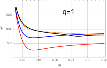
Figure 1: Nonspinning case, $q=1$. Comparison betweeen different representations of the derivative of the phase of the Fourier transform, $-\Psi^{\prime}(f)$. The plot shows: (i) the standard 3.5PN Taylor F2 approximant (blue); (ii) the parametrized 4.5PN one with $c_{22}^{\rm 4PN}=0$ (red); the tuned parametrized 4.5PN one with $c_{22}^{\rm 4PN}=-200$ (orange, dashed); (iii) the phase derivative of the IMRPhenomD model Khan et al. (2016) (black). A single parameter is able to improve the consistency between $T_{\rm F2}^{\rm 4.5PN}$ and IMRPhenomD even below the standard Schwarzschild LSO frequency $Mf_{\rm LSO}^{\rm Schw}\approx 0.0217$.

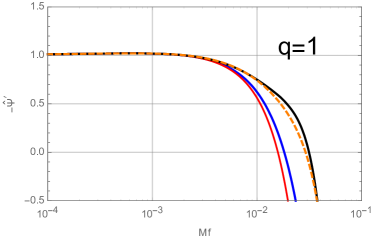
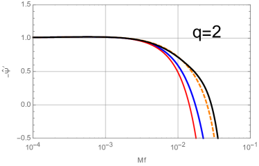
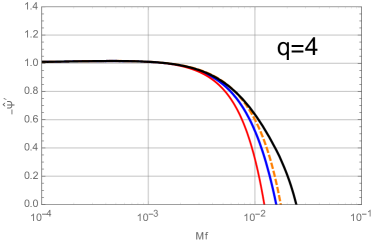
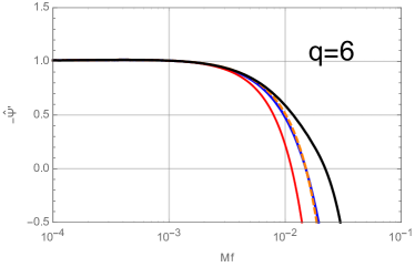
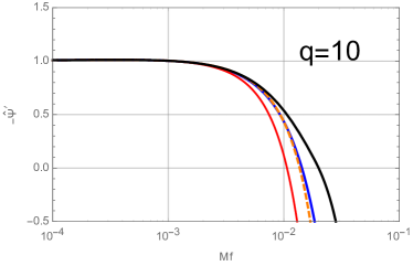
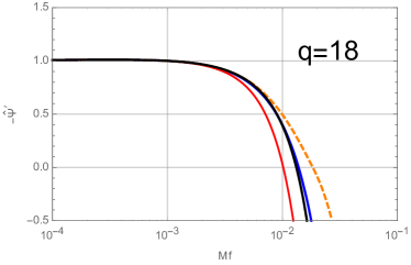
Figure 2: Qualitative exploration of the flexibility of the parametrized, nonspinning, 4.5PN Taylor F2 approximant. The figure shows the Newton-normalized derivative of the frequency-domain phase for mass ratios $q=(1,2,4,6,10,18)$, Eq. (30), computed for: (i) the IMRPhenomD phase (black); (ii) the 3.5PN approximant (blue); (iii) the 4.5PN approximant without tuning (red), $c_{22}^{\rm 4PN}=c_{21}^{\rm 4PN}=0$; (iv) the 4.5PN approximant with $c_{21}^{\rm 4PN}=0$ and $c_{22}^{\rm 4PN}$ tuned so to obtain an accurate representation the IMRPhenomD phase on the largest possible frequency interval.

As a straightforward application of our calculation of the flux at (parametrized) 4.5PN we can compute the corresponding Taylor F2 frequency domain approximant, using the SPA, to the phase of the Fourier transform of the signal. Here, as an exploratory, proof-of-principle, investigation, we only focus on the phase of the Fourier transform and do not discuss the amplitude. The TaylorF2 frequency-domain waveform phase up to 4.5PN reads

$$\Psi_{4.5}^{\rm F2}(f) =2\pi ft_{c}-\varphi_{c}-\dfrac{\pi}{4}$$

$$+\dfrac{3}{128\nu}(\pi fM)^{-5/3}\sum_{i=0}^{9}\varphi_{i}(\pi fM)^{i/3},$$ (27)

where the $\varphi_{i}$’s with $i={0,1,\dots,7}$ are given by the nonspinning limit of Eqs. (B6)-(B13) Ref. Khan et al. (2016). The additional 4PN (parametrized) and 4.5PN (exact) terms read

$$\varphi_{8} =[1-\log(\pi Mf)]\biggl{[}c_{21}^{\rm 3PN}\biggl{(}\frac{40\nu}{81}-\frac{160\nu^{2}}{81}\biggr{)}+\frac{160c_{22}^{\rm 4PN}\nu}{9}-\frac{369469478275\nu^{4}}{16019011008}+\frac{510041481025\nu^{3}}{13106463552}$$ (28)

$$+\biggl{(}\frac{300600673165997}{576684396288}-\frac{399545\pi^{2}}{27216}\biggr{)}\nu^{2}+\biggl{(}-\frac{5679872289503527}{1281520880640}-\frac{5322928\gamma}{3969}+\frac{9302215\pi^{2}}{54432}$$

$$-\frac{1420688\log(2)}{441}+\frac{26325\log(3)}{49}\biggr{)}\nu-\frac{90490\pi^{2}}{567}-\frac{36812\gamma}{189}+\frac{2550713843998885153}{830425530654720}-\frac{26325\log(3)}{196}$$

$$-\frac{1011020\log(2)}{3969}\biggr{]}+\biggl{(}\frac{2661464\nu}{11907}+\frac{18406}{567}\biggr{)}\log^{2}(\pi Mf),$$

$$\varphi_{9} =\pi\bigg{(}-\frac{13696}{63}\log(\pi Mf)+\frac{10323755\nu^{3}}{199584}+\frac{45293335}{127008}\nu^{2}+\left(\frac{2255\pi^{2}}{6}-\frac{1492917260735}{134120448}\right)\nu-\frac{640\pi^{2}}{3}-\dfrac{13696}{21}\gamma_{\rm E}$$

$$+\frac{105344279473163}{18776862720}-\frac{27392}{21}\log(2)\bigg{)}.$$ (29)

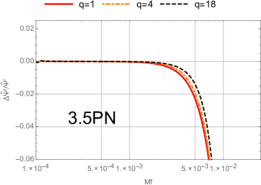
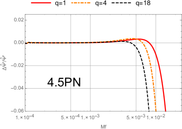
Figure 3: Relative differences between IMRPhenomD and TaylorF2 PN approximants: the 3.5PN disagreement is reduced with the 4.5PN tuned approximant, especially for nearly equal-mass binaries.

In this way we have constructed an approximant that, though dependent on some unknown analytical information, it incorporates in fully consistent way 4PN and 4.5PN terms with the complete $\nu$ dependence. The residual ignorance only resides in the functions $c_{22}^{\rm 4PN}(\nu)$ and $c_{21}^{\rm 4PN}(\nu)$ that parametrize currently unknown 4PN waveform terms. A priori, one is expecting these functions to be just third-order polynomials in $\nu$ by induction from the previous PN orders, since the highest power of $\nu$ that can appear coincides with the highest PN order considered (recall that the quantities that appear in the fluxes are $\nu c_{\ell m}^{\rm 4PN}(\nu)$). Note that, even before the 4PN waveform calculation will be completed, it would be in principle possible to constrain $(c_{22}^{\rm 4PN}(\nu),c_{21}^{\rm 4PN}(\nu))$ by comparing parametrized EOB predictions with NR waveform data, a line of research that worths being investigated in detail in the future. More modestly, here we try to illustrate the usefulness of the new terms in Eqs. (28)-(IV) by presenting a simple comparison between: (i) the new 4.5PN-accurate, parametrized, TaylorF2 approximant; (ii) the usual 3.5PN accurate approximant; (iii) the IMRPhenomD phenomenological model of Fourier phasing of Ref. Khan et al. (2016). This model is calibrated to hybrid EOB-NR waveforms and is able to yield an accurate representation of our best description of the actual phasing (for spinning, nonprecessing, BBHs) from inspiral to plunge, merger and ringdown on a large portion of the (nonprecessing) BBH parameter space. During the inspiral (more precisely, up to $Mf=0.018$), it is built by flexing the standard 3.5PN Taylor F2 approximant by adding effective, parameter-dependent, high-order PN terms that complement the 3.5PN analytical knowledge for both the Fourier phase and amplitude. The terms that are added to do so are effectively some $(\varphi_{8},\varphi_{9},\varphi_{10},\varphi_{11})$. The difference with our case is that no partial analytical knowledge is assumed on them; rather, these terms are determined by fitting to the Fourier transform of suitably computed EOB-NR hybrid waveforms. The IMRPhenomD model was proved to be faithful against a large portion of the currently available Simulating eXtreme Spacetimes (SXS) catalog SXS of NR waveforms; for this reason, in this work we assume it is delivering the “exact” representation of the Fourier phasing (certainly for $Mf\geq 0.0035$, that is the minimum frequency considered for doing the phenomenological fits, see Sec. VIA of Khan et al. (2016)), and thus we use it as a benchmark for the various PN approximant. We compare the derivative of the phase of the Fourier transform with respect to the frequency, $-\Psi^{\prime}(f)\equiv-\partial\Psi(f)/\partial f$, since this is the quantity that was directly calibrated to the hybrid waveforms in Ref. Khan et al. (2016) for technical reasons. For simplicity, we do so by putting $t_{c}=0$ both in the definition of $\Psi_{4.5}^{\rm F2}$, Eq. (IV) above as well as in the IMRPhenomD model. Figure 1 contrasts four representations of $-\Psi^{\prime}(f)$ for the equal-mass, $q=1$ case  The black line is the IMRPhenomD function; the blue is the standard 3.5PN TaylorF2 approximant, while the red is the 4.5PN approximant with $c_{22}^{\rm 4PN}=0$. Not surprisingly, this latter is neither better nor worse than the 3.5PN. However, we find that by considering $c_{22}^{\rm 4PN}$ as an effective, tunable, parameter it is fairly easy to lower the red curve in the figure and to move it on top of the black one during the inspiral. Interestingly, the agreement remains good also after $fM\approx 0.02$. We remind, as a useful mnemonic reference point, that the GW frequency of the Schwarzschild last-stable-orbit (LSO) is $(Mf)_{\rm LSO}^{\rm GW}=\pi^{-1}6^{-3/2}\approx 0.0217$. Note however that for an equal-mass, nonspinning system the LSO, as defined within the EOB approach, occurs at higher frequencies because of the $\nu$-dependent terms in the interaction potential Buonanno and Damour (1999). The orange-dashed curve in Fig. 1 is obtained by fixing $c_{22}^{\rm 4PN}=-200$ (note in this respect that for $\nu=1/4$ the $c_{21}^{\rm 4PN}$-dependent term just vanishes in Eq. (28)). One then finds that the parametrized 4.5PN approximant is sufficiently robust to allow one to obtain similar results also for larger values of $q$: keeping $c_{21}^{\rm 4PN}=0$ for simplicity, it is always possible to find a value of $c_{22}^{\rm 4PN}$ that reduces the gap between the 4.5PN and the IMRPhenomD curves in a frequencies interval where the 3.5PN approximant is not reliable anymore. To quantify this effect, it is useful to look at the Newton-normalized derivative of the phase

$$\hat{\Psi}^{\prime}(f)=\Psi^{\prime}(f)\left(\dfrac{5}{128(fM)^{8/3}\pi^{5/3}\nu}\right)^{-1},$$ (30)

In Fig. 2 we show this quantity for six values of the mass ratio $q$ that belong to the domain of calibration of IMRPhenomD Khan et al. (2016). We use as lower frequency limit $fM=0.0001$. As in Fig. 1, the figure compares four curves: the IMRPhenomD (black); the TaylorF2 at 3.5PN (blue); the untuned TaylorF2 at 4.5PN ($c_{22}^{\rm 4PN}=c_{21}^{\rm 4PN}=0$); the $c_{22}^{\rm 4PN}$-tuned TaylorF2 at 4.5PN. The parameter is determined by hand so to find good consistency with the black curve on the largest possible frequency interval: this is done by inspecting the (relative) difference with $\psi^{\prime}(f)$ yielded by the IMRPhenomD model and tuning $c_{22}^{\rm 4PN}$ so that this difference remains flat on the largest possible frequency interval (see below). Figure 2 illustrates several points: (i) the low-frequency consistency between all PN approximants as well as IMRPhenomD; (ii) neither the 3.5PN-accurate nor the untuned 4.5PN-accurate TaylorF2 deliver accurate approximations to the IMRPhenomD inspiral phasing after frequency $fM\approx 0.005$; (iii) by tuning only the parameter $c_{22}^{\rm 4PN}$ one can easily put the 4.5PN curves on top of the IMRPhenomD for all configurations and the good agreement is kept essentially up to $fM\approx 0.01$ for all binaries (or even to $fM\approx 0.2$ for $q\simeq 1$) except for $q=18$, where the consistency is trustable up to $fM\approx 0.005$. The good values of $c_{22}^{\rm 4PN}(q)$ yielding such behaviors for $q=(1,2,3,4,6,7,10,18)$ are $c_{22}^{\rm 4PN}=(-200,-290,-390,-480,-650,-750,-1050,-2000)$. The improvement brought by the 4.5PN tuned approximant with respect to the purely analytical 3.5PN one is quantitatively illustrated in Fig. 3, that shows the relative differences with the IMRPhenomD, i.e. $\Delta\Psi^{\prime}/\Psi^{\prime}\equiv(\Psi^{\prime}_{\rm IRMPhenomD}-\Psi^{\prime}_{\rm*PN})/\Psi^{\prime}_{\rm IMRPhenomD}$ and highlights how the region of frequencies reliably covered by the PN approximant is enlarged when the 4.5PN-tuned description is employed. Finally, it is easily found that the “first-guess” values of $c_{22}^{\rm 4PN}$ mentioned above and used in Figs. 2-3 can be well fitted by a rational function of the form

$$c_{22}^{\rm 4PN}(\nu)=c_{1/4}^{\rm 4PN}\dfrac{1+n_{1}(X_{12})^{2}+n_{2}(X_{12})^{4}+n_{3}(X_{12})^{6}}{1+d_{1}(X_{12})^{2}}$$ (31)

where $X_{12}\equiv X_{1}-X_{2}=\sqrt{1-4\nu}$, with $c_{1/4}^{\rm 4PN}=-200.821$, $n_{1}=3.1334$, $n_{2}=-6.4605$, $n_{3}=5.0608$, $d_{1}=-1.0027$.

In principle, this effective representation for $c_{22}^{\rm 4PN}$ can yield a complete 4.5PN TaylorF2 approximant that could replace the purely analytical 3.5PN one for the nonspinning sector. Still, we would like to remain very conservative at this stage and stress that our analysis should be considered mainly qualitative and only marginally quantitative, since it only aims at showing the potentialities of our approach. A more quantitative analysis is beyond the scope of this work, and it should be done, for example, by comparing the parametrized PN approximant with long-inspiral EOB waveforms, in order to further reduce potential uncertainties in the IMRPhenomD model. In this respect, a question that may be interesting to answer is to which accuracy an EOB-tuned 4.5PN approximant can effectively reproduce the EOBNR phasing and up to which value of the total mass (probably higher than the limits given by the 3.5PN one Buonanno et al. (2009)) of the binary it could be used in searches. These questions will hopefully find their answers in future studies.

In addition, we also would like to note that the parametrized 4.5PN (once extended to the spinning case) approximant might possibly be used as a replacement of the phenomenological ansatz given by Eq. (28) of Ref. Khan et al. (2016), so to include more analytic information and possibly simplify the fitting procedures, with less parameters to be determined by fitting. Evidently, in doing so one may investigate whether including $c_{21}^{\rm 4PN}$ might be useful as well as the possible extension of the TaylorF2 approximant up to (parametrized) 5.5PN accuracy, using the parametrized 5PN and 5.5PN terms we derived in Eqs. (II)-(II).

IV.1 Preliminary discussion of the spinning case

Finally, we have also driven a preliminary exploration of the spinning case. First of all, one can incorporate the new term of Eq. (26) in the construction of the spin-aligned TaylorF2 approximant. This would add to the known spin-orbit (non-tail) knowledge up to NNLO, the NLO spin-spin and the LO spin cube Bohe et al. (2013, 2015); Marsat (2015); Marsat et al. (2013). In addition, as we did for the nonspinning case, one can similarly parametrize higher PN spin-dependent terms. In this respect, we anticipate that, once the computation of the factorized $\rho_{\ell m}$’s will be completed at NNLO spin-orbit Bohe and Marsat (2017) accuracy, one will have immediate access to some of the higher order tail terms in the flux, so that it will be possible to incorporate a lot of higher PN information in any PN-expanded approximant, though with some dependence on parameters for the uncalculated terms in the $\rho_{\ell m}$’s. However, it will be necessary to investigate carefully to which extent these terms have to be incorporated in a TaylorF2 approximant aiming at being better than the 3.5PN one for small-mass binaries and/or to improve current phenomenological models. By doing a preliminary investigation of the $\hat{\Psi}^{\prime}(f)$ quantity we discussed above, it is easy to find that, when the spins are present (whatever value), the 3.5PN one is monothonically growing after frequencies $fM\approx 0.02$, while the “true” behavior captured by the IMRPhenomD model is actually qualitatively the same as the nonspinning case discussed above, i.e. monothonically decreasing for $fM>0$. Such growing behavior is mainly related to the $\log(\pi Mf)$ term in the $\varphi_{5}$ coefficient of the TaylorF2 approximant, see Eq. (B11) of Ref. Khan et al. (2016). One finds that, if only the LO spin-orbit and spin-spin terms, that is Eqs. (B9) and (B10) of Ref. Khan et al. (2016), are retained in the TaylorF2, together with the same 3.5PN-accurate orbital pieces, the behavior of $\hat{\Psi}^{\prime}(f)$ is qualitatively correct, i.e. it is monotonically decresing with $fM$. We checked this to be the case explicitly for a sample of equal-mass, equal-spin binaries with $-1\leq\chi_{i}\leq 1$. As an instructive exercise, we then built a new, parametrized, TaylorF2 approximant that is formally 4.5PN accurate in the orbital part, but only retains LO spin-orbit and spin-spin terms. Focusing only on the equal-mass, equal-spin case for simplicity, we find it possible, by just flexing the $c_{22}^{\rm 4PN}$ parameter, to have the 4.5PN curve consistent with the IMRPhenomD one up to higher frequencies than those possible for the usual TaylorF2 at 3.5PN. This results illustrates at the same time the robustness and the flexibility of our approach, although more precise and quantitative assessment are needed and are postponed to future studies.

V Conclusions

By Taylor expanding well-known analytical information incorporated in the effective-one-body description of BBHs, we have: (i) shown that the 4.5PN accurate tail-induced flux term obtained by Ref. Marchand et al. (2016) using the multipolar post-minkowskian formalism is already incorporated in the currently used EOB flux and does not need any additional information to be obtained; (ii) we similarly obtained the next-to-leading-order tail-induced spin-orbit term in the flux Marsat et al. (2014); (iii) we have computed for the first time (to our knowledge) the leading-order spin-square tail-induced term, finding perfect agreement with the test-particle limit results of Tagoshi et al. (1996); (iv) we have derived new 4.5PN-accurate (and higher) TaylorF2 approximants that explicitly depend on yet uncalculated PN information. We have illustrated that, thanks to the possibility of flexing a single parameter and focusing on the nonspinning case for simplicity, one is able to reproduce the derivative of the Fourier phase as provided by the IMRPhenomD model up to $fM\approx 0.01$, while the 3.5PN approximants usually stops at $fM\approx 0.005$.

We note in passing that our 4.5PN approximant, once complemented by the 7.5PN accurate tidal phase of Ref. Damour et al. (2012), should yield a better representation of the phasing for nonspinning binary neutron stars (BNS) during the late inspiral, and up to merger, than the 3.5PN one. We recall in fact (see e.g. Fig. 1 of Ref. Bernuzzi et al. (2015)) that the BNS merger frequency, estimated using NR simulations over a large sample of EOS, approximately occurs in the range $0.015\approx Mf_{\rm mrg}^{\rm BNS}\approx 0.032$. In this frequency range, the tuned 4.5PN TaylorF2 is closer to the IMRPhenomD phasing than the standard 3.5PN one (see top-left panel of Fig. 2 and left panel of Fig. 3) and thus it might be helpful to reduce possible systematics yielded by this latter.

In conclusion, our exploratory investigation suggests that EOB-derived, high-order, parametrized, PN-approximants may help to produce improved descriptions of the inspiral phasing that might be useful either for improving current phenomenological models in the low-frequency regime, or even as alternative detection tools for low-mass binaries.

Appendix A Orbital angular momentum at 4PN

Let us briefly recall how the 4PN-accurate expression of the orbital angular momentum given in Eq. (II) can be computed by just PN expanding one of the EOB equations of motion. Our starting point is the 4PN-accurate EOB interaction potential

$$A =1-2u+2\nu u^{3}+a_{4}\nu u^{4}$$ (32)

$$+\nu\left(\frac{64}{5}\log u+a_{5}^{c_{0}}+\nu a_{5}^{c_{1}}\right)u^{5}$$

with $a_{4}=94/3-41/32\,\pi^{2}$, $a_{5}^{c_{0}}=-4237/60+128/5\gamma_{\rm E}+2275/512\,\pi^{2}+256/5\log(2)$ and $a_{5}^{c_{1}}=41/32\pi^{2}-221/6$. The angular momentum along circular orbits is given by Buonanno and Damour (1999)

$$j_{\rm adiab}^{2}(u)=\frac{-A^{\prime}(u)}{(u^{2}A(u))^{\prime}},$$ (33)

where the prime stands for derivative with respect to $u$. From the circularized EOB Hamiltonian

$$\hat{H}=\frac{1}{\nu}\sqrt{1+2\nu\left[\sqrt{A(u)(1+j^{2}u^{2})}-1\right]},$$ (34)

the dimensionless orbital frequency $\hat{\Omega}\equiv GM\Omega/c^{3}$ reads

$$\hat{\Omega}=\frac{\partial{\hat{H}}}{\partial{j}},$$ (35)

which finally yields an expression of $\Omega$ as a function of $u$. We must then invert the series to obtain, from Eq. (33), the orbital angular momentum in terms of the gauge-invariant parameter $x\equiv\hat{\Omega}^{2/3}$ as given in Eq. (II) in the main text.

References

- Buonanno and Damour (1999) A. Buonanno and T. Damour, Phys. Rev. D59, 084006 (1999).
- Buonanno and Damour (2000) A. Buonanno and T. Damour, Phys. Rev. D62, 064015 (2000).
- Damour (2001) T. Damour, Phys. Rev. D64, 124013 (2001).
- Buonanno et al. (2006) A. Buonanno, Y. Chen, and T. Damour, Phys. Rev. D74, 104005 (2006), arXiv:gr-qc/0508067 .
- Damour et al. (2002) T. Damour, E. Gourgoulhon, and P. Grandclement, Phys.Rev. D66, 024007 (2002), arXiv:gr-qc/0204011 [gr-qc] .
- Damour and Nagar (2007) T. Damour and A. Nagar, Phys. Rev. D76, 064028 (2007), arXiv:0705.2519 [gr-qc] .
- Damour et al. (2008) T. Damour, A. Nagar, E. N. Dorband, D. Pollney, and L. Rezzolla, Phys.Rev. D77, 084017 (2008), arXiv:0712.3003 [gr-qc] .
- Abbott et al. (2016a) B. P. Abbott et al. (Virgo, LIGO Scientific), (2016a), arXiv:1602.03840 [gr-qc] .
- Abbott et al. (2016b) B. P. Abbott et al. (Virgo, LIGO Scientific), (2016b), arXiv:1602.03841 [gr-qc] .
- Abbott et al. (2016c) B. P. Abbott et al. (Virgo, LIGO Scientific), Phys. Rev. Lett. 116, 061102 (2016c), arXiv:1602.03837 [gr-qc] .
- Abbott et al. (2016d) B. P. Abbott et al. (Virgo, LIGO Scientific), Phys. Rev. Lett. 116, 241103 (2016d), arXiv:1606.04855 [gr-qc] .
- Abbott et al. (2016e) B. P. Abbott et al. (Virgo, LIGO Scientific), Phys. Rev. X6, 041015 (2016e), arXiv:1606.04856 [gr-qc] .
- Khan et al. (2016) S. Khan, S. Husa, M. Hannam, F. Ohme, M. Puerrer, X. Jimenez Forteza, and A. Bohe, Phys. Rev. D93, 044007 (2016), arXiv:1508.07253 [gr-qc] .
- Buonanno et al. (2009) A. Buonanno, B. Iyer, E. Ochsner, Y. Pan, and B. Sathyaprakash, Phys.Rev. D80, 084043 (2009), arXiv:0907.0700 [gr-qc] .
- Bini and Damour (2013) D. Bini and T. Damour, Phys.Rev. D87, 121501 (2013), arXiv:1305.4884 [gr-qc] .
- Damour et al. (2016) T. Damour, P. Jaranowski, and G. Schafer, Phys. Rev. D93, 084014 (2016), arXiv:1601.01283 [gr-qc] .
- Damour et al. (2015) T. Damour, P. Jaranowski, and G. Schafer, Phys. Rev. D91, 084024 (2015), arXiv:1502.07245 [gr-qc] .
- Damour et al. (2014) T. Damour, P. Jaranowski, and G. Schaefer, Phys.Rev. D89, 064058 (2014), arXiv:1401.4548 [gr-qc] .
- Bernard et al. (2016) L. Bernard, L. Blanchet, A. Bohe, G. Faye, and S. Marsat, Phys. Rev. D93, 084037 (2016), arXiv:1512.02876 [gr-qc] .
- Bernard et al. (2017) L. Bernard, L. Blanchet, A. Bohe, G. Faye, and S. Marsat, Phys. Rev. D95, 044026 (2017), arXiv:1610.07934 [gr-qc] .
- Damour and Nagar (2009) T. Damour and A. Nagar, Phys. Rev. D79, 081503 (2009).
- Damour and Nagar (2014) T. Damour and A. Nagar, Phys.Rev. D90, 044018 (2014), arXiv:1406.6913 [gr-qc] .
- Balmelli and Damour (2015) S. Balmelli and T. Damour, Phys. Rev. D92, 124022 (2015), arXiv:1509.08135 [gr-qc] .
- Damour et al. (2009) T. Damour, B. R. Iyer, and A. Nagar, Phys. Rev. D79, 064004 (2009).
- Damour et al. (2012) T. Damour, A. Nagar, and L. Villain, Phys.Rev. D85, 123007 (2012), arXiv:1203.4352 [gr-qc] .
- Marchand et al. (2016) T. Marchand, L. Blanchet, and G. Faye, Class. Quant. Grav. 33, 244003 (2016), arXiv:1607.07601 [gr-qc] .
- Marsat et al. (2014) S. Marsat, A. Bohe, L. Blanchet, and A. Buonanno, Class. Quant. Grav. 31, 025023 (2014), arXiv:1307.6793 [gr-qc] .
- Faye et al. (2015) G. Faye, L. Blanchet, and B. R. Iyer, Class. Quant. Grav. 32, 045016 (2015), arXiv:1409.3546 [gr-qc] .
- Pan et al. (2011) Y. Pan, A. Buonanno, R. Fujita, E. Racine, and H. Tagoshi, Phys.Rev. D83, 064003 (2011), arXiv:1006.0431 [gr-qc] .
- Tagoshi et al. (1996) H. Tagoshi, M. Shibata, T. Tanaka, and M. Sasaki, Phys. Rev. D54, 1439 (1996), arXiv:gr-qc/9603028 [gr-qc] .
- (31) http://www.black-holes.org/waveforms.
- Bohe et al. (2013) A. Bohe, S. Marsat, and L. Blanchet, Class. Quant. Grav. 30, 135009 (2013), arXiv:1303.7412 [gr-qc] .
- Bohe et al. (2015) A. Bohe, G. Faye, S. Marsat, and E. K. Porter, Class. Quant. Grav. 32, 195010 (2015), arXiv:1501.01529 [gr-qc] .
- Marsat (2015) S. Marsat, Class. Quant. Grav. 32, 085008 (2015), arXiv:1411.4118 [gr-qc] .
- Marsat et al. (2013) S. Marsat, L. Blanchet, A. Bohe, and G. Faye (2013) arXiv:1312.5375 [gr-qc] .
- Bohe and Marsat (2017) A. Bohe and S. Marsat, (2017), in preparation.
- Bernuzzi et al. (2015) S. Bernuzzi, A. Nagar, T. Dietrich, and T. Damour, Phys.Rev.Lett. 114, 161103 (2015), arXiv:1412.4553 [gr-qc] .