Charmonium spectrum with a Dirac potential model in the momentum space

Abstract

We study the charmonium spectrum using a complete one gluon exchange approach based on a phenomenological relativistic $q\bar{q}$ potential model with Dirac spinors in momentum space. We use phenomenological screening factors to include vacuum quantum effects. Our formulation does not rely on nonrelativistic approximations. We fit the lowest-lying charmonia (below the $D\bar{D}$ threshold) and predict the higher-lying resonances of the spectrum. In general, we reproduce the overall structure of the charmonium spectrum and, in particular, we can reasonably describe the $X(3872)$ resonance mass as (mostly) a $c\bar{c}$ state. The numerical values of the free parameters of the model are determined taking into account also the experimental uncertainties of the resonance energies. In this way, we are able to obtain the uncertainties of the theoretical resonance masses and the correlation among the free parameters of the model.

I Introduction

In the last years the interest in charmonia has been renewed by the experimental observation of new charmoniumlike states Olsen1 ; brambilla ; Godfrey:2008nc ; Esposito:2016noz ; Swanson1 ; Esposito:2014rxa ; Lebed . Some of these states have been easily identified as charmonia, e.g. $h_{c}(1P)$ Rosner ; Rubin and $\chi_{c2}(2P)$ Uehara , as reported by the Particle Data Group (PDG) PDG2016 . However there exist other important resonances that are still under examination. These states, denoted as $X$, $Y$ and $Z$, do not match the predictions of the nonrelativistic or semirelativistic $q\bar{q}$ potential models and some of them have been described as tetraquarks, molecules, glueballs and hybrids Olsen1 ; brambilla ; Esposito:2016itg ; Brodsky:2014xia ; Godfrey:2008nc ; Pilloni:2015doa ; Esposito:2016noz ; Lebed ; Guo:2008yz ; Guo-Galata ; Ber-Brambi ; Faccini:2013lda . Another possible explanation suggests that some of these states may be the result of kinematic effects Szczepaniak:2015eza ; Guo:2014iya that appear in the nearby of the thresholds of the open charm channels. The interpretation of these resonances depends, to a certain extent, on the theoretical approach that is followed to perform the amplitude analysis of the data Pilloni:2016obd ; Kang:2016jxw and to study charmonium spectroscopy.

Quantum chromodynamics (QCD) must be considered, in any case, the underlying field theory for the study of these systems. However, due to the difficulty of finding analytically (approximated) solutions for QCD, alternative approaches have been followed. For example, numerical lattice QCD (LQCD) Liu:2012ze ; Christopher ; Lang ; Gunnar , potential quark models Isgur ; Capstick ; Faustov ; DeSanctis2 ; Cao2012 ; DeSanctis3 ; klink ; poly ; Bram-Gro ; Kawanai1 ; Laschka ; PhysRevD.85.091503 ; Kawanai2 , unquenched quark models (UQM) Santo ; Santo2 ; Ferre-Galata ; FeSa1 ; FeSa2 ; FeSa3 , and Bethe-Salpeter approaches Hilger:2015hka ; Fischer ; Popovici .

LQCD represents a very promising but, at the same time, highly difficult tool. LQCD computations reproduce the structure of the charmonium spectrum and predict many undiscovered states Liu:2012ze ; Christopher ; Gunnar . In particular, LQCD is computationally taxing, especially when open channels and the resonant nature of the states are considered, and still needs to be improved in order to reproduce accurately the hadron spectrum Luscher ; Rummukainen ; Briceno1 ; Briceno2 ; Dudek:2012xn ; mesonsector ; Wilson ; Dudek . Exploratory LQCD simulations of the $D\bar{D}$ scattering in S and P waves have been recently computed Lang but they still need to be improved to achieve the precision of the lowest-energy meson sector Briceno:2016mjc . However, the construction of potential quark models whose interaction has been derived from LQCD Kawanai1 ; Laschka ; PhysRevD.85.091503 ; Kawanai2 , building up models that are not purely phenomenological Bali:2000gf , has proved to be a very useful tool for the study of these physical systems. Historically, the Cornell potential Eichen represents the first interaction that was introduced, with partial success, to study the charmonium spectrum. This model consists of a Coulomb-like potential and a linear term inserted in a standard nonrelativistic Schrödinger equation. The Coulomblike term takes into account reduction of the one gluon exchange (OGE) in the short range region. The linear term introduces quark confinement in the model, in approximate agreement with the spectroscopy of the first excited states. LQCD studies have confirmed the presence of the linear term in the long range effective interaction PhysRevD.85.091503 . However, in this model, the nonrelativistic approximation cannot be really justified and the fine structure of the spectrum, related to the spin-spin, spin-orbit and tensor interactions, has to be introduced by hand in a purely phenomenological way. Furthermore, higher order effects of the field theory reduction are also absent.

Throughout the literature several relativized quark models have been introduced in order to incorporate some relativistic effects Isgur ; Capstick ; Faustov ; DeSanctis2 ; Cao2012 ; DeSanctis3 ; klink ; poly ; Bram-Gro . A possible approach to include some of the relativistic effects in a consistent way is given by the generalization of the Fermi-Breit expansion (originally studied for the electromagnetic interaction) followed in DeSanctis2 ; Cao2012 ; DeSanctis3 to study the resonant states of strongly interacting quarks. We point out that this approach is not fully relativistic because the interaction terms are expanded in powers of $p/m$, where $p$ and $m$ are the quark momentum and mass, respectively. These models also assume that the mean values of $p/m$ are small and, consequently, only the first terms of the expansion are retained. The obtained effective interaction, by means of a Fourier transform, can be expressed in the coordinate space in terms of local operators. As a consequence, the eigenvalue equation for the effective Hamiltonian of these models can be solved with the standard techniques. For the specific case of relativized quark models for hadronic systems, the Bakamjian-Thomas construction may be used in the context of relativistic Hamiltonian dynamics klink ; poly . This approach allows us to perform exact Lorentz boosts on the wave functions of the model, but no connection between the interaction Hamiltonian and the Dirac structure of the underlying theory can be easily established. In other words, one cannot express the interaction of the model in terms of the Dirac covariants that are the building blocks of any relativistic theory, i.e. the scalar, vector, pseudoscalar, tensor and pseudotensor terms. Further details can be found in klink ; poly .

Another approach to improve the dynamical description of the quarkonium spectrum consists in employing the UQM formalism. In the UQM, starting from a relativized quark model, the coupling of the valence quarks to the continuum is taken into account through a self energy term Santo ; Santo2 ; Ferre-Galata . This coupling causes a shift in the energy, generally leading to a reduction in the masses of the quarkonia FeSa1 ; FeSa2 ; FeSa3 in the high-lying states. This effect can also be incorporated, in a more phenomenological way, through the screening of the interaction potential Li ; Gonzalez which produces a similar global result.

It is also possible to perform a four-dimensional fully relativistic computation of the heavy meson spectra solving the Bethe-Salpeter equation. This approach has been taken in the context of the rainbow ladder approximation Hilger:2015hka . This approach presents relevant theoretical advantages; however, the quality of the theoretical spectrum is not completely satisfactory and, in particular, spurious states are obtained Fischer ; Popovici as a consequence of the adopted dynamical approximations Ahlig ; Bijtebier1 .

In the present work we develop a relativistic model inspired by the OGE interaction. In our calculation we do not perform any nonrelativistic expansion. Hence, the well-known spin-orbit, spin-spin and tensor effects are automatically given by the relativistic calculation. Due to the Dirac structure of the interaction, the model is necessarily constructed in the momentum space. We include vector and scalar interaction terms as well as phenomenological screening factors Li ; Gonzalez ; Bai . We solve an integral eigenvalue Hamiltonian equation in the momentum space through a variational method and we perform the diagonalization of the Hamiltonian matrix in a selected orthonormal basis. We determine the parameters of the model by fitting the low-lying charmonia states taking into account the experimental uncertainties. These uncertainties are exactly propagated to the parameters and to the computed spectrum using the bootstrap technique NumericalRecipes ; Landay:2016cjw . This method is computationally expensive but allows a rigorous determination, from the statistical point of view, of the parameters of the model and their uncertainties, as well as the propagation of such uncertainties to the computation of the spectrum. The rigorous study of the uncertainties allows to identify the statistically significant differences between the theoretical and the experimental spectra, determining which states are in need of physics beyond the $c\bar{c}$ picture to be described. Moreover, the method allows to study the correlations among the parameters of the model, which provides insight on how physically independent are the different pieces that build the phenomenological model. As far as we know, no previous works on phenomenological models of charmonia have addressed the problem of rigorously establishing the correlations among parameters, the associated uncertainties of the parameters and their impact in the predicted spectrum.

The paper is organized as follows. In Section II we develop the general structure of our theoretical model. In particular, we show the details of the vector and scalar interactions that we use to obtain the charmonium spectrum. In Section III we discuss the methods used to solve the eigenvalue equation and to determine the free parameters of the model and their uncertainties. We also show how these uncertainties are propagated to the energy levels of the theoretical charmonium spectrum. In Section IV we provide our results compared to the available experimental data and we discuss different phenomenological interpretations. Finally, in Section V we summarize the results of the study. The details on the spin-angle matrix elements are left for Appendix A.

II Theoretical model

In this section we provide a detailed description of our theoretical model for the study of charmonium spectroscopy. The model consists in a three-dimensional reduction of the Bethe-Salpeter equation in which only the contributions of the positive energy Dirac spinors of the quarks are retained. Dirac spinors guarantee that relativity is satisfied and the Dirac structure of the interaction is highlighted. Due to the relativistic nature of the model, the well-known spin-orbit, spin-spin and tensor effects are all automatically included in our calculation. If we expand our model in powers of $p/m$ we recover the standard semirelativistic Fermi-Breit interaction Lifshitz .

II.1 Definitions

As it is customary, we work in the center of mass (CM) reference frame of the $c\bar{c}$ system and we use the system of natural units ($\hbar=c=1$). The quantities of the ket and bra states are labeled with the indices $a$ and $b$, respectively. Hence, the three-momentum of the quark (particle 1) and the three-momentum of the antiquark (particle 2) are written as

$$\begin{split}\vec{p}_{1a}&=-\vec{p}_{2a}=\vec{p}_{a},\\ \vec{p}_{1b}&=-\vec{p}_{2b}=\vec{p}_{b},\end{split}$$ (1)

where the relative three-momenta $\vec{p}_{b}$ and $\vec{p}_{a}$ are the actual kinematic variables employed in the calculations. We also introduce the three-momentum transfer

$$\vec{q}=\vec{p}_{b}-\vec{p}_{a},$$ (2)

and the cosine of the angle between $\vec{p}_{a}$ and $\vec{p}_{b}$

$$x=\cos\theta=\hat{p}_{a}\cdot\hat{p}_{b},$$ (3)

so that

$$\vec{q}^{\>2}=\vec{p}_{a}^{\>2}+\vec{p}_{b}^{\>2}-2p_{a}p_{b}x,$$ (4)

where $p_{a}$ and $p_{b}$ are the moduli of the respective three-momenta, $\hat{p}_{a}=\vec{p}_{a}/p_{a}$ and $\hat{p}_{b}=\vec{p}_{b}/p_{b}$. The on shell energies of both particles ($i=1,2$) are

$$\begin{split}E(\vec{p}_{ia})=E(\vec{p}_{a})=\sqrt{\vec{p}_{a}^{\>2}+m^{2}},\\ E(\vec{p}_{ib})=E(\vec{p}_{b})=\sqrt{\vec{p}_{b}^{\>2}+m^{2}},\end{split}$$ (5)

where $m$ stands for the quark and antiquark masses. We introduce the energy difference (for both particles) between the bra and ket states

$$\Delta E=E(\vec{p}_{b})-E(\vec{p}_{a}),$$ (6)

and the invariant four-momentum transfer squared ($Q^{2}>0$)

$$Q^{2}=\vec{q}^{\>2}-(\Delta E)^{2}.$$ (7)

Finally, for completeness, we give the standard definition of the positive energy Dirac spinors that will be used in the calculation

$$u(\vec{p}_{i},\vec{\sigma}_{i})=\sqrt{\frac{E(\vec{p}_{i})+m}{2E(\vec{p}_{i})}}\begin{pmatrix}1\\ \frac{\vec{p}_{i}\cdot\vec{\sigma}_{i}}{E(\vec{p}_{i})+m}\end{pmatrix}\chi,$$ (8)

where $i=1,2$ is the particle index, $\vec{\sigma}_{i}$ are the Pauli matrices and $\chi$ represents a generic two component spin wave function. Using Eq. (1), we take $\vec{p}_{i}=\vec{p}_{ia}$ and $\vec{p}_{i}=\vec{p}_{ib}$, for the ket and bra states, respectively. The spinors are normalized to ${u}^{{\dagger}}(\vec{p}_{i},\vec{\sigma}_{i})u(\vec{p}_{i},\vec{\sigma}_{i})=1$.

II.2 Total interaction Hamiltonian and screening factors

The matrix elements of the total Hamiltonian in momentum space are obtained adding two terms that represent the vector and the scalar interactions

$$\bar{\cal H}_{\text{int}}(\vec{p}_{b},\vec{p}_{a})=\langle\vec{p_{b}}|H^{(v)}|\vec{p_{a}}\rangle+\langle\vec{p_{b}}|H^{(s)}|\vec{p_{a}}\rangle,$$ (9)

where, for brevity, the spin matrices have not been explicitly written. However, the standard phenomenological potentials do not allow for a good reproduction of the spectrum, in particular above the open charm threshold Li ; Vija-Gon-Gar . A more complete dynamical treatment is necessary. Some of the vacuum quantum effects predicted by QCD can be taken into account by unquenching the quark model as in bijker ; ref ; Ferretti:2015fba . In particular, the virtual pair creation effects are incorporated to the Hamiltonian, i.e, the contribution given by the coupling of the $c\bar{c}$ states to the meson-meson continuum Santo ; Santo2 . Below threshold, this coupling to the continuum states gives rise to virtual $q\bar{q}-q\bar{q}$ components in the meson wave function that shift the charmonia Santo2 and bottomonia FeSa1 ; FeSa2 ; FeSa3 masses through a self-energy term. Part of these virtual pair production effects can be taken into account, in a more phenomenological way, introducing a screening factor in the confinement interaction in the coordinate space Li ; Gonzalez .

In this work, we introduce this screening effect phenomenologically, incorporating momentum dependent factors in the interaction Hamiltonian as follows

$$\bar{\cal H}_{\text{int}}(\vec{p}_{b},\vec{p}_{a})\rightarrow{\cal H}_{\text{int}}(\vec{p}_{b},\vec{p}_{a})=F_{s}(p_{b})\bar{\cal H}_{\text{int}}(\vec{p}_{b},\vec{p}_{a})F_{s}(p_{a}),$$ (10)

where the factors $F_{s}(p_{a})$ and $F_{s}(p_{b})$ take into account the screening effect. In the present work we use the following stepwise function to describe such screening effects

$$F_{s}(p)=\frac{1+k_{s}}{k_{s}+\exp{\left(p^{2}/p^{2}_{s}\right)}},$$ (11)

where $k_{s}$ and $p_{s}$ will be determined (as the rest of the parameters of the model) by fitting to the lowest energy levels of the charmonium spectrum. The details on the fit are provided in Section III.2.

II.3 Vector interaction

In the Coulomb gauge, the vector interaction matrix element reads

$$\langle\vec{p}_{b}|H^{(v)}|\vec{p}_{a}\rangle=\alpha\left(J^{0}_{1}\>J^{0}_{2}\>D_{00}+J^{\alpha}_{1}\>J^{\beta}_{2}\>D_{\alpha\beta}\right).$$ (12)

If we choose $\alpha=\alpha_{em}$ (the electromagnetic fine structure constant) we obtain the standard electromagnetic interaction whose expansion up terms $p/m$ gives the Fermi-Breit interaction Lifshitz . We generalize the previous equation to the strong interaction between a quark and an antiquark DeSanctis2 . In particular, $J^{\mu}_{i}$ represents the quark ($i=1$) and antiquark ($i=2$) Dirac four-current that will be given explicitly in Eq. (17). Furthermore

$$D_{00} =-\frac{1}{\vec{q}^{\>2}},$$ (13)

$$D_{\alpha\beta} =\frac{1}{Q^{2}}\left(\delta_{\alpha\beta}-\frac{q_{\alpha}q_{\beta}}{\vec{q}^{\>2}}\right).$$ (14)

Given that we use positive energy Dirac spinors, we can write the continuity equation in the form

$$(\Delta E)\>J^{0}_{1,2}=\pm\>\vec{q}\cdot\vec{J}_{1,2},$$ (15)

where the signs $+$ and $-$ correspond to the quark and antiquark cases respectively. Using Eq. (15) we can rewrite Eq. (12) for the strong interaction as

$$\begin{split}\langle\vec{p_{b}}|H^{(v)}|\vec{p_{a}}\rangle=&\>V^{(v)}(\vec{q})\>\left[J^{0}_{1}\>J^{0}_{2}\left(1-\frac{(\Delta E)^{2}}{Q^{2}}\right)\right.\\ &-\left.\vec{J}_{1}\cdot\vec{J}_{2}\left(1+\frac{(\Delta E)^{2}}{Q^{2}}\right)\right].\end{split}$$ (16)

The explicit form of the effective vector potential $V^{(v)}(\vec{q})$ is provided in Eq. (20a) of Section II.5. Notice that, compared to Eq. (12), we take $\alpha=\alpha_{st}$, which represents the phenomenological strong coupling constant of the model.

Finally, the quark and antiquark four-currents are given by the standard form

$$J_{i}^{\mu}=J_{i}^{\mu}(\vec{\sigma}_{i};\vec{p}_{b},\vec{p}_{a})=\bar{u}(\vec{p}_{ib},\vec{\sigma}_{i})\gamma_{i}^{\mu}u(\vec{p}_{ia},\vec{\sigma}_{i}).$$ (17)

In this work we do not include a chromomagnetic current term, which seems to be unnecessary given the quality of the obtained spectrum as shown in Section IV.

II.4 Scalar interaction

In hadron spectroscopy the spin-obit effect is in general rather small and cannot be reproduced if we only use a vector interaction. Hence, a scalar interaction, partially responsible for quark confinement Swanson1 ; Swanson2 , is included in the interaction Hamiltonian to improve the description of the charmonium spectrum Cao2012 ; Ebert . Also in the present work we find that the scalar interaction is needed to obtain a good description of the charmonium spectrum. We write the scalar interaction in the following standard way

$$\langle\vec{p}_{b}|H^{(s)}|\vec{p}_{a}\rangle=V^{(s)}(\vec{q})\>I_{1}\>I_{2},$$ (18)

with the explicit form of the effective scalar potential $V^{(s)}(\vec{q})$ provided in Eq. (20b) of Section II.5. The scalar vertex is given by

$$I_{i}=I_{i}(\vec{\sigma}_{i};\vec{p}_{b},\vec{p}_{a})=\bar{u}(\vec{p}_{ib},\vec{\sigma}_{i})u(\vec{p}_{ia},\vec{\sigma}_{i}).$$ (19)

II.5 Vector and scalar potentials

In order to include different physical effects in our effective interaction, it is necessary to use phenomenological expressions for the potentials in momentum space. There exist a wide range of models for the scalar and vector potentials DeSanctis2 ; Faustov ; Radford . In this work we use the following effective potentials:

$$V^{(v)}(\vec{q})=-\frac{4}{3}\frac{\alpha_{st}}{\vec{q}^{\>2}}+\beta_{v}\frac{3b^{2}-\vec{q}^{\>2}}{(\vec{q}^{\>2}+b^{2})^{3}},$$ (20a)

$$V^{(s)}(\vec{q})=A+\beta_{s}\frac{3b^{2}-\vec{q}^{\>2}}{(\vec{q}^{\>2}+b^{2})^{3}}.$$ (20b)

We note that only by a combination of scalar and vector confining potentials is it possible to eliminate the empirically contraindicated spin-orbit interaction in the interquark potential. The vector interaction, Eq. (20a), is given by a regularized Cornell potential in momentum space where the $-\frac{4}{3}\alpha_{st}/\vec{q}^{\>2}$ term in Eq. (20a) corresponds to the standard pure Coulombian strong potential, being $\alpha_{st}$ the effective strong coupling constant and $\frac{4}{3}$ the color factor. The second term corresponds to a confining interaction where the $\beta_{v}$ parameter is related to the vector confinement intensity. The parameter $b$ has been introduced to avoid the $1/{q}^{4}$ singularity in the momentum space interaction and, in the present model, has no direct physical meaning. The expression of the vector potential in the coordinate space reads

$$V^{(v)}(r)=-\frac{4}{3}\frac{\alpha_{st}}{r}+\beta_{v}\pi^{2}r\exp{(-rb)},$$ (21)

where it is apparent that the second term represents a linear confinement interaction regularized with a decreasing exponential function. For convenience, we fix $b=10^{-2}~{}\text{GeV}$, that corresponds to $1/b\simeq 20~{}\text{fm}$. The $b$ value is chosen small enough to avoid numerical problems and large enough to approximately recover the Cornell potential for the energy region of interest. Regarding the scalar interaction in Eq. (20b), we take a phenomenological constant term, represented by $A$, plus a linear regularized potential, analogous to the confining term of the vector potential. We note that $\beta_{s}$ is (as $\beta_{v}$) related to the confinement strength, and we also fix $b=10^{-2}~{}\text{GeV}$. In this work we use two different prescriptions for the scalar potentials to fit the experimental data. In the first prescription (potential I), we set $\beta_{s}=0$, i.e. we keep the effective constant scalar confinement term $A$ in Eq. (20b) and we omit the scalar linear regularized potential. In the second one (potential II), the value of $\beta_{s}\neq 0$ is determined fitting the data. We study these two prescriptions separately in order to assess the impact of the confinement term of the scalar interaction. In what follows we refer to these two models as

$$\begin{cases}\text{potential I\phantom{I}}\rightarrow\text{model using Eqs.~{}(\ref{vtotq}) with }\beta_{s}=0,\\ \text{potential II}\rightarrow\text{model using Eqs.~{}(\ref{vtotq}) with }\beta_{s}\neq 0.\end{cases}$$ (22)

II.6 Integral equation for the $c\bar{c}$ system

Now, we can write the total integral Hamiltonian equation (in momentum space) for our system. First, we introduce the standard kinetic energy of the quark and the antiquark in the charmonium CM

$$K(\vec{p})=2\sqrt{\vec{p}^{\>2}+m^{2}}.$$ (23)

The integral Hamiltonian equation takes the form

$$[K(\vec{p_{b}})+M_{0}]\Psi(\vec{p}_{b})+\int d^{3}p_{a}{\cal H}_{\text{int}}(\vec{p}_{b},\vec{p}_{a})\Psi(\vec{p}_{a})=M\>\Psi(\vec{p}_{b}),$$ (24)

where ${\cal H}_{\text{int}}(\vec{p}_{b},\vec{p}_{a})$ is given by Eq. (9), $M_{0}$ represents a phenomenological zero point energy of the spectrum, $M$ is the resonance mass (that is the eigenvalue of the integral equation) and $\Psi(\vec{p})$ is the resonance wave function. For brevity, in the interaction Hamiltonian, the Pauli spin matrices have not been explicitly written and also, in the wave function, the energy and angular momentum quantum numbers have been omitted.

Equation (24) can be obtained performing a three-dimensional reduction of a Bethe-Salpeter equation with an instantaneous interaction and projecting the result onto the positive energy spinors itzy .

III Solution method and fitting procedure

III.1 Solution method

In order to determine the resonance energies of the spectrum we have to solve Eq. (24) which is a Fredholm integral equation of second order Arfken . There are different available methods to solve this kind of integral equations. In particular, we employ a variational procedure. First, we express the wave function of the system by means of a superposition of the wave functions of a given trial basis. Using the standard $LS$ coupling for the angular momenta the wave functions read

$$\Psi_{n,\{\nu\}}(\vec{p})=R_{n,L}(p;\bar{p})\left[Y_{L}(\hat{p})\otimes\chi_{S}\right]_{J,M_{J}},$$ (25)

where the radial function in the momentum space $R_{n,L}(p;\bar{p})$ represents the trial function, $n$ is the principal quantum number, $\bar{p}$ is the variational parameter with the dimension of momentum, $Y_{L,M_{L}}(\hat{p})$ is the corresponding spherical harmonic, and $\chi_{S,M_{S}}$ is the spin function. For convenience we introduce the shorthand notation $\{\nu\}=L,S,J$ for the spin-angle quantum numbers of the basis, i.e., the orbital angular momentum ($L$), the total spin ($S=0,1$) and the total angular momentum ($J$). For the actual calculations we take the projection of the total angular momentum on the $z$-axis as $M_{J}=J$. The matrix elements involving other values of $M_{J}$ are related to the $M_{J}=J$ matrix element through the Wigner-Eckart theorem edmonds . For simplicity we do not consider the possibility that different values of $L$ mix, whose effect has been shown to be negligible in semirelativistic models Radford ; DeSanctis2 . For the radial part we select the orthonormal three dimensional harmonic oscillator wave functions

$$R_{n,L}(p;\bar{p})=\left[\frac{2n!}{\Gamma(n+L+\frac{3}{2})}\right]^{\frac{1}{2}}\frac{s^{L}}{\bar{p}^{\frac{3}{2}}}{\cal L}^{L+\frac{1}{2}}_{n}(s^{2})\exp{\left[\frac{-s^{2}}{2}\right]},$$ (26)

where ${\cal L}^{L+\frac{1}{2}}_{n}(s^{2})$ are the generalized Laguerre polynomials, $s\equiv p/\bar{p}$ and $\bar{p}$ is the variational parameter. Now, we can diagonalize the Hamiltonian (mass) matrix in Eq. (24) obtaining

$$M_{\{\nu\},n_{b},n_{a}}=M_{0}\delta_{n_{b},n_{a}}+\int d^{3}p\>\Psi_{n_{b},\{\nu\}}^{{\dagger}}(\vec{p})K(\vec{p})\Psi_{n_{a},\{\nu\}}(\vec{p})+\int d^{3}p_{b}\>d^{3}p_{a}\Psi_{n_{b},\{\nu\}}^{{\dagger}}(\vec{p_{b}}){\cal H}_{\text{int}}(\vec{p}_{b},\vec{p}_{a})\Psi_{n_{a},\{\nu\}}(\vec{p_{a}}),$$ (27)

where, as before, the Pauli spin matrices in ${\cal H}_{\text{int}}(\vec{p}_{b},\vec{p}_{a})$ have not been explicitly written. Notice that a six-dimensional integration over $\vec{p}_{b}$ and $\vec{p}_{a}$ appears in the interaction term. We integrate analytically the spin-angle part of the matrix elements (see details in Appendix A) so that only a three-dimensional integration over $p_{b}$, $p_{a}$ and $\cos\theta=x$ is left.

To solve Eq. (27) we use the variational diagonalization procedure introduced in DeSanctis2 . We obtain good numerical convergence for the energy eigenvalues taking the first ten trial wave functions of the basis for each state. Hence, the $10\times 10$ Hamiltonian matrix is diagonalized and minimized through the standard variational approach. Once a numerical solution is obtained, we check that the solution represents a good numerical approximation. We substitute the numerical solution in the lhs of Eq. (24) and verify that it fulfills the integral equation.

III.2 Fitting and uncertainties calculation

The two models under study defined by potentials I and II, see Eq. (22), depend on seven and eight parameters respectively. Potential I depends on $m$ (constituent mass of the $c$ and $\bar{c}$ quarks), $M_{0}$ (phenomenological zero point energy of the spectrum), $\alpha_{st}$ (effective strong coupling constant), $\beta_{v}$ (vector confinement intensity), $A$ (constant scalar interaction), and $k_{s}$ and $p_{s}$ (screening parameters), while the model with potential II depends on the same parameters plus $\beta_{s}$ that represents the scalar confinement intensity.

To determine the values of the parameters, the corresponding uncertainties and the charmonium spectrum we fit the experimental resonance masses given in Table 1, i.e. the ground states of each $J^{PC}$ band plus the $\eta_{c}^{\prime}$ and $\psi^{\prime}$ resonances, whose energies are below the open charm threshold $D\bar{D}$. In doing so, we proceed as follows Fernandez-Ramirez:2015fbq :

1. We randomly choose values for the masses of the resonances by sampling a Gaussian distribution according to the uncertainties given in Table 1, obtaining a resampled lowest-lying charmonia spectrum;

2. We use the least-squares method to minimize the squared distance

   $$d^{2}=\sum_{i}\left(E_{i}-M_{i}\right)^{2},$$ (28)

   where $M_{i}$ represent these resampled ground state experimental masses, i.e. the lowest-lying states with quantum numbers: $i\equiv J^{PC}=$ $0^{-+}$ ($\eta_{c}$ and $\eta^{\prime}_{c}$), $1^{--}$ ($J/\psi$ and $\psi^{\prime}$), $0^{++}$ ($\chi_{c0}$), $1^{+-}$ ($h_{c}$), $1^{++}$ ($\chi_{c1}$) and $2^{++}$ ($\chi_{c2}$), and $E_{i}$ are the theoretical CM energies of the lowest-lying states obtained from the potential models I and II solving Eq. (27). The fits are performed using MINUIT MINUIT .

Table 1: Fitted charmonia for potentials I and II compared to the experimental masses from PDG. $n$ stands for the principal quantum number, $L$ for the orbital angular momentum, $J$ for the total angular momentum and $S$ for the spin.

Name	$n\>^{2S+1}L_{J}$	Masses (MeV)
		Potential I	Potential II	Experiment
$\eta_{c}$	$1\>^{1}S_{0}$	$\phantom{0}2990^{+6}_{-12}$	$\phantom{0}2981^{+8}_{-12}$	$\phantom{0}2983.6\pm 0.6$
$J/\psi$	$1\>^{3}S_{1}$	$3089.3^{+5.7}_{-6.5}$	$\phantom{0}3101^{+13}_{-10}$	$\phantom{0}3096.916\pm 0.011$
$\chi_{c0}$	$1\>^{3}P_{0}$	$3417.0^{+8.4}_{-5.9}$	$\phantom{0}3416^{+11}_{-13}$	$\phantom{0}3414.75\pm 0.31$
$\chi_{c1}$	$1\>^{3}P_{1}$	$3500.7^{+4.4}_{-3.4}$	$3506.3^{+7.7}_{-7.1}$	$\phantom{0}3510.66\pm 0.07$
$h_{c}$	$1\>^{1}P_{1}$	$3514.9^{+5.9}_{-4.6}$	$3521.0^{+6.5}_{-6.7}$	$\phantom{0}3525.38\pm 0.11$
$\chi_{c2}$	$1\>^{3}P_{2}$	$\phantom{0}3579^{+5}_{-12}$	$\phantom{0}3563^{+8}_{-14}$	$\phantom{0}3556.20\pm 0.09$
$\eta_{c}^{\prime}$	$2\>^{1}S_{0}$	$\phantom{0}3646^{+7}_{-12}$	$\phantom{0}3647^{+10}_{-12}$	$\phantom{0}3639.2\pm 1.2$
$\psi^{\prime}$	$2\>^{3}S_{1}$	$3674.9^{+5.4}_{-5.7}$	$3679.2^{+9.2}_{-9.4}$	$3686.109^{+0.012}_{-0.014}$

This procedure is repeated $1000$ times providing enough statistics to compute the expected value of the parameters and the spectrum energies as well as their uncertainties at a $1\sigma$ (68%) confidence level (CL). The expected values of the parameters are computed as the mean values of the $1000$ samples. To compute the uncertainties at a $1\sigma$ CL we take the best 68% of the fits and we compute the differences between the mean value and the highest and lowest masses. In this way our uncertainties are not symmetric. Table 2 provides the fitted parameters for both potentials and Tables 3 and 4 the correlation matrices of the parameters for potentials I and II, respectively.

Table 2: Fit parameters for the two potentials considered in this work. Error bars are reported at the 1$\sigma$ (68%) CL and take into account all the correlations among parameters (see Section III.2).

Parameter	Potential I	Potential II
$m$ (MeV)	$1455^{+30}_{-26}$	$1364^{+46}_{-63}$
$M_{0}$ (MeV)	$\phantom{0}108^{+21}_{-25}$	$\phantom{0}270\pm 45$
$\alpha_{st}$	$\phantom{00}0.63^{+0.08}_{-0.06}$	$\phantom{0}0.544^{+0.027}_{-0.060}$
$\beta_{v}$ (GeV2)	$\phantom{0}0.0134^{+0.0009}_{-0.0014}$	$\phantom{0}0.004^{+0.001}_{-0.002}$
$k_{s}$	$\phantom{00}59^{+11}_{-9}$	$\phantom{0}96^{+14}_{-10}$
$p_{s}$ (GeV)	$\phantom{0}0.698^{+0.065}_{-0.067}$	$\phantom{0}0.91^{+0.11}_{-0.06}$
$A$ (GeV-2)	$\phantom{00}0.015\pm 0.004$	$-0.006\pm 0.002$
$\beta_{s}$ (GeV2)	$\phantom{00}0$ (fixed)	$\phantom{0}0.013^{+0.004}_{-0.003}$

Table 3: Correlation matrix for the parameters of potential I.

	$m$	$M_{0}$	$\alpha_{st}$	$\beta_{v}$	$k_{s}$	$p_{s}$	$A$
$m$	$\phantom{-}1$
$M_{0}$	$-0.78$	$\phantom{-}1$
$\alpha_{st}$	$\phantom{-}0.86$	$-0.40$	$\phantom{-}1$
$\beta_{v}$	$-0.88$	$\phantom{-}0.39$	$-0.93$	$\phantom{-}1$
$k_{s}$	$\phantom{-}0.11$	$-0.02$	$\phantom{-}0.13$	$-0.23$	$\phantom{-}1$
$p_{s}$	$\phantom{-}0.33$	$-0.34$	$\phantom{-}0.05$	$-0.16$	$-0.62$	$\phantom{-}1$
$A$	$-0.76$	$\phantom{-}0.59$	$-0.53$	$\phantom{-}0.62$	$\phantom{-}0.03$	$-0.70$	$\phantom{-}1$

Table 4: Correlation matrix for the parameters of potential II.

	$m$	$M_{0}$	$\alpha_{st}$	$\beta_{v}$	$k_{s}$	$p_{s}$	$A$	$\beta_{s}$
$m$	$\phantom{-}1$
$M_{0}$	$-0.61$	$\phantom{-}1$
$\alpha_{st}$	$\phantom{-}0.40$	$\phantom{-}0.31$	$\phantom{-}1$
$\beta_{v}$	$-0.12$	$\phantom{-}0.04$	$\phantom{-}0.06$	$\phantom{-}1$
$k_{s}$	$\phantom{-}0.31$	$-0.10$	$\phantom{-}0.14$	$-0.23$	$\phantom{-}1$
$p_{s}$	$\phantom{-}0.02$	$-0.20$	$-0.42$	$-0.17$	$-0.35$	$\phantom{-}1$
$A$	$\phantom{-}0.22$	$-0.18$	$\phantom{-}0.09$	$-0.21$	$\phantom{-}0.24$	$\phantom{-}0.58$	$\phantom{-}1$
$\beta_{s}$	$-0.29$	$-0.20$	$-0.52$	$-0.66$	$\phantom{-}0.02$	$\phantom{-}0.33$	$\phantom{-}0.29$	$\phantom{-}1$

Table 3 (potential I), shows a strong correlation among the parameters of the vector interaction in Eq. (20a). Furthermore, we note a marked correlation between $A$ and all the parameters of the vector interaction, confirming that, in this model, vector and scalar interactions are physically correlated. Besides, it is worth highlighting the correlation of the parameters in the vector and scalar interactions with the screening parameters $k_{s}$ and $p_{s}$ of Eq. (11). We notice that the parameter $p_{s}$ turns out to be weakly correlated with the parameters of the vector interaction but strongly correlated with the parameters of the scalar interaction. For potential II, see Eq. (22), we have the additional parameter $\beta_{s}$. In this case the parameters are less correlated among them than for potential I, see Table 4. In particular, we point out that the correlations between the effective quark mass ($m$) and other parameters are significantly reduced in potential II compared to potential I, with the exception of the phenomenological zero point energy $M_{0}$. Also, the correlation between $\alpha_{st}$ and $\beta_{v}$ is largely reduced. In this way, the parameters in the vector interaction are uncorrelated among them. Regarding the scalar interaction, we observe that the parameters $A$ and $\beta_{s}$ are almost uncorrelated. However, we noticed a considerable correlation between parameters $\beta_{v}$ and $\beta_{s}$, suggesting that, in any case, a strong physical correlation exists between the confinement terms of the vector and the scalar interactions. The parameter $p_{s}$ of the screening factors is weakly correlated with the other parameters of the interactions except with the phenomenological parameter $A$ in the scalar interaction. The high correlation highlights how the screening impacts the scalar interaction. Finally, comparing the correlation matrices for both potentials, we find that the addition of the confining term in the scalar interaction reduces the correlation among some of the parameters, which allows for a more straightforward interpretation of the physics associated to each term in the potential.

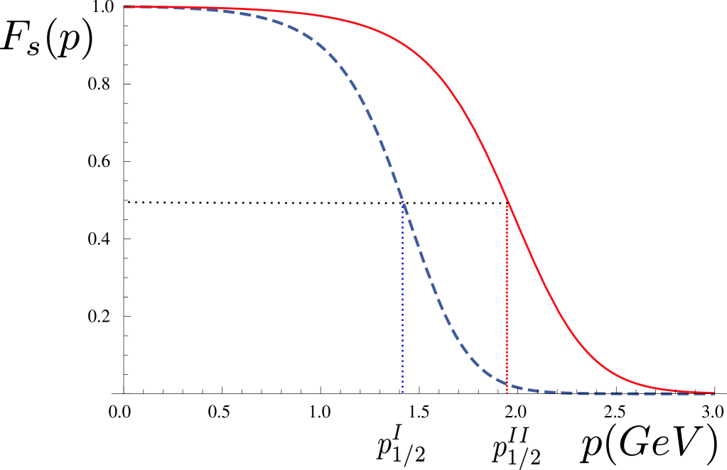
Figure 1: Screening function, Eq. (11), for potentials I (dashed blue) and II (solid red). For $k_{s}$ and $p_{s}$ we use the central values in Table 2. We highlight the values of the screening momenta $p^{\text{I}}_{1/2}$ (potential I) and $p^{\text{II}}_{1/2}$ (potential II) defined in Section III.2.

For completeness, we plot the screening function $F_{s}(p)$ in Fig. 1 for the two potentials. We introduce the screening momentum $p^{\>\text{j}}_{1/2}$ ($\text{j}=\text{I},\text{II}$ labels potentials I and II) that are defined by $F_{s}(p^{\>\text{j}}_{1/2})=1/2$ (recall that $F_{s}(0)=1$). We find the values of $p^{\text{I}}_{1/2}=1.4~{}\text{GeV}$ and $p^{\text{II}}_{1/2}=1.9~{}\text{GeV}$. These values correspond to the screening kinetic energy

$$\bar{E}^{\>\text{j}}=2\sqrt{m^{2}+\left(p^{\>\text{j}}_{1/2}\right)^{\>2}}$$ (29)

obtaining $\bar{E}^{\text{I}}=4.1~{}\text{GeV}$ and $\bar{E}^{\text{II}}=4.7~{}\text{GeV}$. It shows that the screening effect is active above the open charm threshold where a sort of saturation energy must be introduced for the interaction Xiang .

We now consider the specific calculation of the charmonium spectrum and its theoretical uncertainties. Once that $1000$ fits have been performed, the uncertainties of the model parameters can be propagated to the charmonium spectrum using bootstrap NumericalRecipes ; Landay:2016cjw . This method allows us to carry to the spectrum computation the experimental uncertainties together with the correlations among the parameters. This method is more accurate than those using the covariance matrix, although it is computationally more expensive. In more detail, the computation of the charmonium spectrum is performed as follows: For each one of the $1000$ sets of parameters obtained from the fits we compute the spectrum. Hence, for each state of the spectrum we have a set of $1000$ values of the mass. The expected value of each state as well as the uncertainty is computed in the same way it was done for the parameters.

IV Results for the charmonium spectrum

Tables 1 (fitted states) and 5 (predicted states) report the obtained spectra for both models. Figures 2 (potential I) and 3 (potential II) provide a graphical representation of our results compared to the available experimental data from PDG PDG2016 . We can see that the obtained fits (below open charm threshold) are excellent and that, in general, the whole spectrum is well described with both potentials. We note that the statistical uncertainties grow up with the excitation energy of the states.

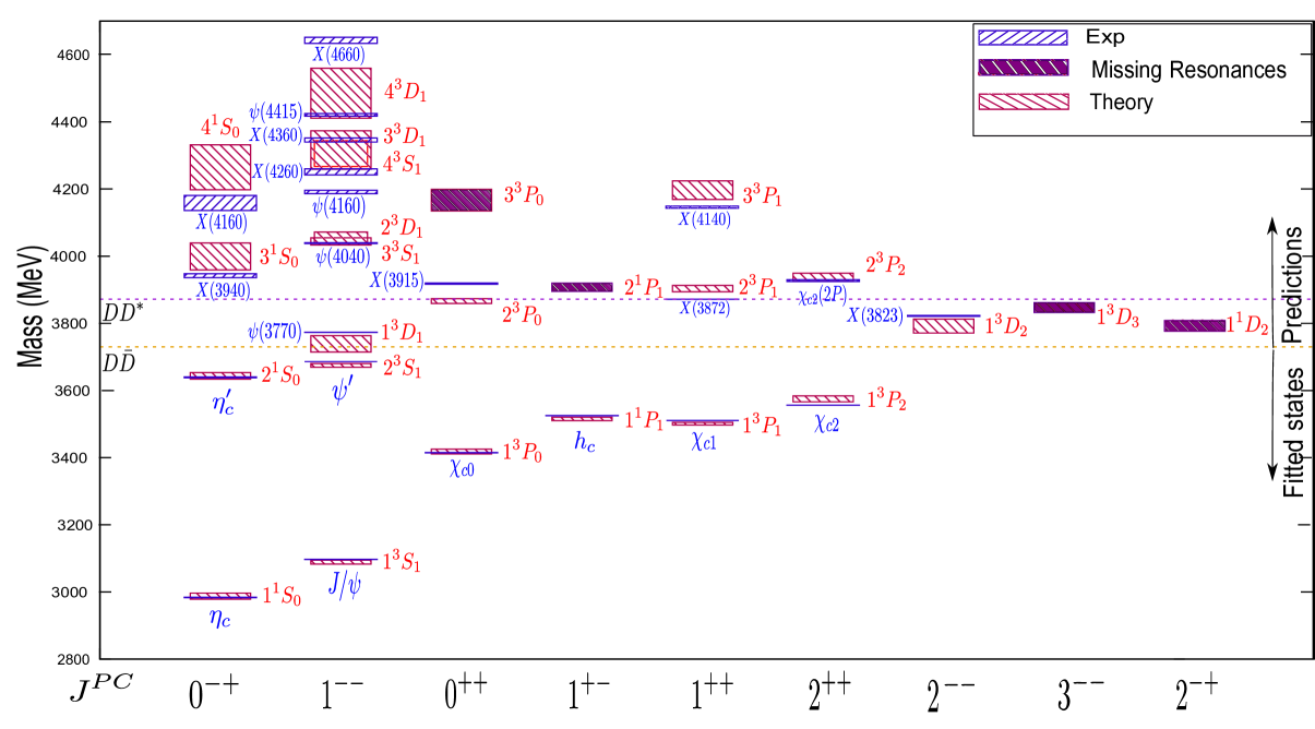
Figure 2: Complete charmonium spectrum obtained with potential I (red boxes) compared to the experimental spectrum from PDG (blue boxes). The size of the red boxes accounts for error bars at 1$\sigma$ (68%) CL. In the same way, the size of the blue boxes stands for the experimental error of the resonance masses. The dashed lines stand for the open charm energies $D\bar{D}$ and $DD^{*}$. The calculation of the uncertainties takes into account all the correlations among the parameters (see Section III.2 for details). In the horizontal axis the quantum numbers $J^{PC}$ are reported for the states above. In the right side of the figure, the arrows indicate the states (below the $D\bar{D}$ threshold) that are used in the fitting procedure and the predictions of the model with potential I. It is important to note that we have used the latest nomenclature by the PDG where the vector mesons are also named as $X$ instead of $Y$ as it is commonplace in the charmonia research field. The states in both naming schemes relate as follows: $Y(4260)\leftrightarrow X(4260)$, $Y(4360)\leftrightarrow X(4360)$, $Y(4660)\leftrightarrow X(4660)$, $Y(4140)\leftrightarrow X(4140)$ and $Y(3915)\leftrightarrow X(3915)$.

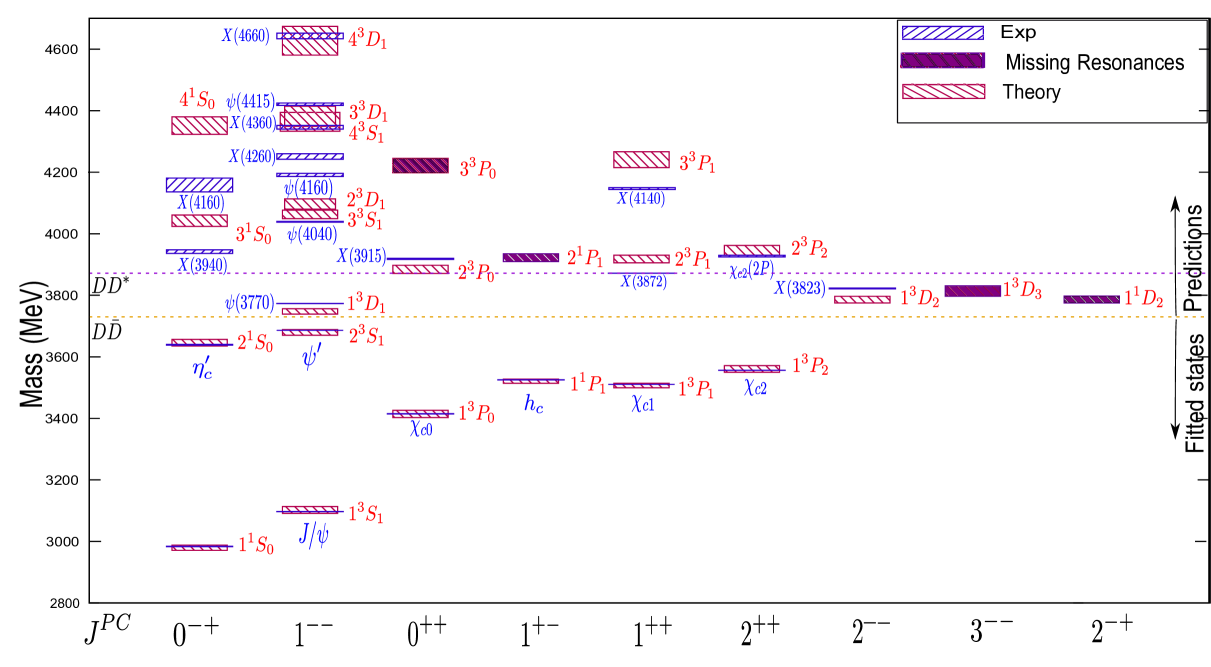
Figure 3: Charmonium spectrum obtained with potential II. Notation as in Fig. 2.

Table 5: Predicted charmonia for potentials I and II compared to the experimental masses and uncertainties from PDG. Notation as in Table 1. For the $X(4160)$ experimental mass the first error is statistical and the second systematic Abe:2007sya .

Name	$n\>^{2S+1}L_{J}$	Mass (MeV)
		Potential I	Potential II	Experiment
—	$1\>^{1}D_{2}$	$\phantom{0}3788^{+20}_{-12}$	$3789^{+9}_{-13}$	—
$\psi(3770)$	$1\>^{3}D_{1}$	$\phantom{0}3723^{+41}_{-8}$	$3749^{+7}_{-10}$	$3773.13\pm 0.35$
$\psi(3823)$	$1\>^{3}D_{2}$	$\phantom{0}3782^{+30}_{-11}$	$3788^{+9}_{-12}$	$3822.2\pm 1.2$
—	$1\>^{3}D_{3}$	$\phantom{0}3849^{+13}_{-17}$	$3817^{+14}_{-20}$	—
$X(3915)$ [$Y(3915)$]	$2\>^{3}P_{0}$	$3867.9^{+5.5}_{-8.6}$	$3884^{+14}_{-13}$	$3918.4\pm 1.9$
—	$2\>^{1}P_{1}$	$\phantom{0}3908^{+11}_{-13}$	$3923^{+11}_{-13}$	—
$X(3872)$	$2\>^{3}P_{1}$	$3903.5^{+9.3}_{-9.4}$	$3918^{+13}_{-12}$	$3871.69\pm 0.17$
$\chi_{c2}(2P)$	$2\>^{3}P_{2}$	$\phantom{0}3941^{+8}_{-16}$	$3945^{+17}_{-14}$	$3927.2\pm 2.6$
$\psi(4160)$	$2\>^{3}D_{1}$	$\phantom{0}4059^{+13}_{-20}$	$4094^{+19}_{-20}$	$4191\pm 5$
$X(3940)$	$3\>^{1}S_{0}$	$\phantom{0}4030^{+9}_{-71}$	$4043^{+18}_{-19}$	$3942\pm 6$
$\psi(4040)$	$3\>^{3}S_{1}$	$\phantom{0}4046^{+9}_{-13}$	$4060^{+17}_{-11}$	$4039\pm 1$
—	$3\>^{3}P_{0}$	$\phantom{0}4182^{+17}_{-47}$	$4219^{+26}_{-21}$	—
$X$(4140) [$Y$(4140)]	$3\>^{3}P_{1}$	$\phantom{0}4200^{+24}_{-31}$	$4238^{+29}_{-22}$	$4146.9\pm 3.1$
$X(4160)$	$4\>^{1}S_{0}$	$\phantom{00}4300^{+30}_{-100}$	$4349^{+31}_{-26}$	$4156^{+25}_{-20}\pm 15$

Table 6: Predicted states that can be interpreted differently depending on the potential model. Notation as in Table 1.

Name	Potential	$n\>^{2S+1}L_{J}$	Mass (MeV)
			Theory	Experiment
$X(4260)$	I	$4^{3}S_{1}$	$4311_{-44}^{+33}$	$4251\pm 9$
$[Y(4260)]$	II	—–
$X(4360)$	I	$3^{3}D_{1}$	$4312_{-53}^{+62}$	$4346\pm 6$
$[Y(4360)]$	II	$4^{3}S_{1}$	$4360_{-28}^{+34}$
$\psi(4415)$	I	$4^{3}D_{1}$	$4489_{-78}^{+65}$	$4421\pm 4$
	II	$3^{3}D_{1}$	$4378_{-29}^{+36}$
$X(4660)$	I	——		$4643\pm 9$
$[Y(4660)]$	II	$4^{3}D_{1}$	$4620_{-39}^{+54}$

Table 1 shows that potential II reproduces all the fitted states within the $1\sigma$ CL while for potential I $\chi_{c1}$ and $\chi_{c2}$ fall marginally outside of the $1\sigma$ CL. Hence, potential II produces a slightly better result for the $J^{PC}$ ground states. If we look into the predicted excited states (Table 5) we see larger differences between both potentials, although the produced overall structure of the spectrum is the same.

In this Section we discuss in more detail some of the states as given by potentials I and II, according to the $n^{2S+1}L_{J}$ spectroscopical assignment of the quantum numbers.

IV.1 $X(3915)$, $X(3872)$ and $\chi_{c2}(2P)$

For these states we assign the quantum numbers $2^{3}P_{J}$, with $J=0$, $1$ and $2$ for $X(3915)$, $X(3872)$ delAmoSanchez:2010jr and $\chi_{c2}(2P)$ respectively. Potentials I and II are able to reproduce the hyperfine splitting of the fitted $1P$ states ($\chi_{c0}$, $h_{c}$, $\chi_{c1}$ and $\chi_{c2}$) but the structure of the $2P$ states cannot be reproduced with the same accuracy. In particular, the fact that the $X(3915)$ state has a higher mass than the $X(3872)$. However, we accurately predict the $\chi_{c2}(2P)$ state within uncertainties with both models. These states lay very close to the $\bar{D}D^{*}$ threshold, hence, dynamical effects and degrees of freedom not considered in our models such as threshold effects and molecular admixture in the wave functions can be responsible for the deviations from our predictions.

The $X(3872)$ state is of particular interest and requires a careful discussion. This resonance was discovered by the Belle collaboration in $B$ decays Choi and was confirmed by CDF collaboration Acosta . Various interpretations have been proposed for this resonance whose properties cannot be easily explained within a standard $q\bar{q}$ picture of mesons due to the proximity to the $\bar{D}D^{*}$ decay threshold Santo2 . It has been identified as a tetraquark Terasaki ; Faustov ; Esposito:2014rxa ; Maiani:2004vq , as a $\bar{D}D^{*}$ molecule Wong ; Baru ; Ortega:2010qq ; AlFiky:2005jd , as $c\bar{c}$ core plus molecular components Santo2 , and as a hybrid state Takizawa . Even in the context of semirelativistic quark models there is certain controversy on the assignment of the quantum numbers. In particular, besides the usual $2^{3}P_{1}$ assignment (favored by studies of the decay processes Faccini:2012zv ; Aaij13 ), a $1^{1}D_{2}$ has also been proposed DeSanctis ; Radford . Within the Bethe-Salpeter approach this resonance has been identified with a $3^{3}P_{1}$ state at a mass value of $3912~{}\text{MeV}$ Fischer but, at the same time, a spurious $2^{3}P_{1}$ state at $3672~{}\text{MeV}$ is also obtained. Other calculations with a similar formalism obtain approximately the mass value of $3900~{}\text{MeV}$, but incorporating the $X(3872)$ state in the fitting procedure Hilger:2014nma . The semirelativistic calculations in DeSanctis ; DeSanctis2 , that employ a vector and a scalar interaction, obtain a mass of $3912~{}\text{MeV}$ for the $2^{3}P_{1}$ state. The UQM obtains a mass value around $3908~{}\text{MeV}$ ref ; Santo2 ; Ferreti_alone ; Ferre-Galata . A calculation in the coordinate space with a screened potential has also given a good result of $3901~{}\text{MeV}$ Bai . In general, the nonrelativistic and semirelativistic quark models tend to overestimate the mass of this resonance with respect to the experimental value Radford ; Cao2012 ; Barnes . In the present work we obtain $3903$ and $3918~{}\text{MeV}$ with potentials I and II, respectively. These results are in reasonable but not complete agreement with the experimental value. This result together with the large isospin violation Olsen1 which prevents the identification of this state with a standard charmonium, indicates the need for a more accurate model that includes, in more precisely way, the threshold effects due to the opening of $D\bar{D}$ and $\bar{D}D^{*}$ channels. Finally, we note that both models predict a $1^{1}D_{2}$ state with mass value of $\approx 3790~{}\text{MeV}$. This resonance has not been experimentally observed yet. To complete the analysis of this multiplet, we comment on the $X(3915)$ resonance. This state has been described as a $c\bar{c}$ state Gang and also has been suggested to be a tetraquark Voloshin and a molecule Molina:2012bz . In the $c\bar{c}$ context, this resonance is identified with the $2^{3}P_{0}$ state Gang . However, there exist some issues that question the validity of this assignment. For example, it has been proposed that the $X(3915)$ is basically the $\chi_{c2}(2P)$ Zhou:2015uva ; Baru:2017fgv Among them we highlight the lack of signal in the $X(3915)\rightarrow D\bar{D}$ decay channel Olsen1 . Furthermore, the energy difference between the mass of the $X(3915)$ and its hyperfine splitting partner $\chi_{c2}(2P)$, is smaller than expected Olsen1 ; Olsen2 ; Xia . In our model the expected values of the mass for the $2^{3}P_{0}$ state are $\approx 45~{}\text{MeV}$ (potential I) and $\approx 20~{}\text{MeV}$ (potential II) below the experimental data. Hence, our model does not describe this state with high accuracy, but taking into account the general uncertainties in the hadronic models, an interpretation of this state as a $c\bar{c}$ meson cannot be excluded.

IV.2 $\psi(3770)$, $\psi(4040)$, $\psi(4160)$ and $\psi(4415)$

In the overpopulated zone of the $J^{PC}=1^{--}$ resonances above the $D\bar{D}$ energy threshold, we find some states that are reported by the PDG as charmonia: $\psi(3770)$, $\psi(4040)$, $\psi(4160)$ and $\psi(4415)$, and generally interpreted as $1^{3}D_{1}$, $3^{3}S_{1}$, $2^{3}D_{1}$ and $4^{3}S_{1}$ states respectively Olsen1 .

In our model, with both potentials, we can reproduce the mass of the $\psi(3770)$ with acceptable accuracy. The minor difference between the theoretical and experimental value ($50~{}\text{MeV}$ with potential I and $20~{}\text{MeV}$ with potential II) can be related to the proximity of the $D\bar{D}$ threshold.

The $\psi(4040)$, with an experimental mass value of $4039~{}\text{MeV}$, is generally identified as a $3^{3}S_{1}$ state Olsen1 ; Lebed . However, the theoretical mass value obtained with potential models for the $3^{3}S_{1}$ state is greater than the experimental value Barnes ; DeSanctis2 ; Cao2012 . In our case we can describe this state with sufficient accuracy thanks to the inclusion of the screening functions Bai . In particular, potential I provides a theoretical prediction that agrees with the experimental value within uncertainties. Potential II also produces an acceptable mass value for this state.

The $\psi(4160)$ is interpreted as a radial excitation of the $\psi(3770)$. The predicted mass value is lower than the experimental one, a situation similar to what happens in other screened potential models Bai ; Vijande . If we accept that the $\psi(4160)$ can be considered as a pure $2^{3}D_{1}$ state, we have to conclude that our model and the screened potential models are unable to reproduce this state, supporting a more elaborated nature for this state Barnes-Close ; Asner_etal .

Finally, the resonance $\psi(4415)$ has been generally interpreted as a $4^{3}S_{1}$ state Olsen1 but also as a $5^{3}S_{1}$ state in Bai where the masses of the $\psi$ states are lowered by the inclusion of the screening effects. Within our model it may be tentatively described in two different ways depending on which potential is used (see Table 6). Potential I suggests that we can roughly identify this resonance with a $4^{3}D_{1}$ state but potential II suggests a $3^{3}D_{1}$ state. These unusual tentative assignments for $\psi(4415)$ differ from the standard ones of the semirelativistic potential models Isgur ; Radford where this resonance is well described as a $4^{3}S_{1}$ state. We note that in our model the $4^{3}S_{1}$ state has a mass of $4311~{}\text{MeV}$ with potential I and $4360~{}\text{MeV}$ with potential II, that are better matches for the $X(4260)$ [$Y(4260)$] and the $X(4360)$ [$Y(4360)$] resonances, respectively. Hence, our $4^{3}S_{1}$ state cannot be identified as the $\psi(4415)$.

IV.3 $X(4260)$, $X(4360)$ and $X(4660)$

These resonances with $J^{PC}=1^{--}$ were discovered by BaBar B.Aubert1 and Belle C.Yuan ; Wang1 collaborations and confirmed by a combined analysis of the data Z.Liu . There exist different interpretations of the nature of these resonances: hybrid charmonia Zhu ; Guo:2008yz , tetraquarks Wang ; Galkin-Fau , molecules Close , $c\bar{c}$ mesons Ding and some authors suggest that these signals are the product of the interference between different channels and resonances Chen0 ; Chen1 ; Chen2 . In the charmonium context, these vector mesons are atypical. Their quantum numbers are univocally determined by their production mechanism but some of their features, e.g. the absence of open charm production Galkin-Fau , do not match the $c\bar{c}$ picture brambilla ; Olsen1 .

Our two potentials produce different results for these states. We note that, in our model, the predictions in the high energy region of the spectrum depend strongly on the form of the scalar interaction. Potential I predicts a $4^{3}S_{1}$ state, i.e. $\psi(4S)$, that can be roughly identified with the $X(4260)$ [$Y(4260)$] resonance. This assignment is reasonable if we compare with the bottomonium system. In particular, we compare the experimental mass difference $\Upsilon(4S)-\Upsilon(3S)\approx 224~{}\text{MeV}$ with that of $\psi(4S)-\psi(3S)\approx 254~{}\text{MeV}$. In Liu-Chen a mass of $\approx 4260~{}\text{MeV}$ was obtained for the $\psi(4S)$ state. Also, as in Bai , in our model we can match the $3^{3}D_{1}$ state to the $X(4360)$ resonance. Finally, we note that potential I cannot reproduce the $X(4660)$ [$Y(4660)$] resonance. Potential II depicts a completely different situation. We identify the resonances $X(4360)$ [$Y(4360)$] and $X(4660)$ with the $4^{3}S_{1}$ and $4^{3}D_{1}$ states respectively but we cannot describe the $X(4260)$ state.

IV.4 $X(3940)$ and $X(4160)$

These states were observed by Belle collaboration in double charm production processes Abe:2007sya ; Abe ; Shen . Their decays suggest the $J^{PC}=0^{-+}$ quantum numbers. They have been described in many different ways: hybrids Petrov , molecules Molina:2009ct ; Fernandez , and as the second ($\eta_{c}^{\prime\prime}$) and the third ($\eta_{c}^{\prime\prime\prime}$) radial excitations of the $\eta_{c}$ meson in a standard $c\bar{c}$ picture KTChao ; Estia ; Ping . Both semirelativistic and nonrelativistic potential models Barnes obtain masses for $\eta_{c}^{\prime\prime}$ and $\eta_{c}^{\prime\prime\prime}$ above the experimental values of $X(3940)$ and $X(4160)$, which casts doubts on these assignments.

In Liu-Chen it is assumed that the energy gap between $\psi(3S)-\psi(2S)\approx 353~{}\text{MeV}$ resonances is similar to the $\eta_{c}(3S)-\eta_{c}(2S)$ gap, making it possible to estimate the energy of $\eta(3S)$. The authors found that $\eta(3S)\approx 3992~{}\text{MeV}$, roughly close to the experimental mass of the $X(3940)$. This allows us to identify it as a $3^{1}S_{0}$ state. On the other hand, through a decay analysis in Liu-Chen it is concluded that it is not possible to identify the $X(4160)$ resonance with a $4^{3}S_{0}$ state.

In the screened potential model Bai the correspondence between the $X(3940)$ resonance and the $3^{1}S_{0}$ state is slightly improved. They found $\eta_{c}(3S)=3991~{}\text{MeV}$, but the difference between the experimental mass of the $X(4160)$ and the theoretical mass value of the $4^{1}S_{0}$ state ($4250~{}\text{MeV}$) is large enough to call into question this assignment. In our model, with potential I and the assignments $3^{1}S_{0}$ and $4^{1}S_{0}$, we obtain the values of $4030~{}\text{MeV}$ and $4302~{}\text{MeV}$ for $X(3940)$ and $X(4160)$, respectively. Using potential II, we obtain for the same states the values of $4043~{}\text{MeV}$ and $4349~{}\text{MeV}$, respectively. We see in Table 5 and in Fig. 2 that with potential I we can obtain a rough description of $X(3940)$. Nevertheless, in general, we conclude that our model is not able to describe appropriately these two resonances.

IV.5 $X(4140)$

This resonance was first observed in Aaltonen1 and later confirmed Aaltonen2 . It has been interpreted as a tetraquark Fang ; Stancu ; Wang:2015pea , as a molecule Wang:2009ue ; Wang:2014gwa ; Xiang , as a hybrid charmonium Mahajan and as a $c\bar{c}$ state Gonzalez . Recently, the LHCb collaboration Aaij reported the $1^{++}$ quantum numbers for this resonance, which leads to a $3^{3}P_{1}$ state interpretation, i.e. $\chi_{c1}(3P)$, within the $c\bar{c}$ context Chen:2016iua . The mass value of the $3^{3}P_{1}$ state in the relativistic potential Barnes and screened potential Bai models is above of the mass of the $X(4140)$ [$Y(4140)$] resonance, but, for the case of the latter the difference is just $40~{}\text{MeV}$, so this interpretation is possible. In our case, the $3^{3}P_{1}$ state is obtained with higher values than the experimental data found by LHCb for both potentials. More precisely, potentials I and II predict this state approximately $30~{}\text{MeV}$ and $70~{}\text{MeV}$ above the experimental value, respectively.

IV.6 $\psi(3823)$

This resonance was observed for the first time more than 20 years ago Antoni . Recently, it was observed again by Belle collaboration Bhardwaj and confirmed by BESIII collaboration Ablikim . In agreement with semirelativistic potential models Barnes ; Radford , our model describes reasonably well this state with both potentials, $\approx 3785~{}\text{MeV}$ versus an experimental value of $3822~{}\text{MeV}$, with the standard assignment $1^{3}D_{2}$ ($J^{PC}=2^{--}$). In Bai , it was found a mass value of $3798~{}\text{MeV}$, similar to ours. In the UQM Santo2 a mass of $3736~{}\text{MeV}$ was found, significantly lower than the experimental value.

IV.7 Missing resonances

Our model, as the majority of the $c\bar{c}$ models do, predicts (with both potentials) some states that have not been observed in the experiments yet. In particular, we note the states $1^{1}D_{2}$, $2^{1}P_{1}$, $3^{3}P_{0}$ and $1^{3}D_{3}$. The $1^{1}D_{2}$ state, as already discussed, does not represent a good candidate for the $X(3872)$ and constitutes a missing resonance produced by our model. The $2^{1}P_{1}$ state belongs to an energy region where only the charged mesons $Z_{c}(3900)$ and $Z_{c}(4010)$ have been found. This region is currently empty of charmonialike states, while the radial excitations of the $h_{c}$ state should lie there. The $3^{3}P_{0}$ state that was identified as $X(4140)$ in the past becomes a missing resonance (see Section IV.5) if we consider the latest results from LHCb Aaij . The last missing resonance, the $1^{3}D_{3}$ state, also remains undetected despite that its energy value is close to the open charm threshold.

V Summary and conclusions

We have studied the charmonium spectrum employing a $c\bar{c}$ relativistic Dirac potential model in momentum space with a vector and a scalar interaction. We note that only by a combination of scalar and vector confining potentials is it possible to eliminate the empirically contraindicated spin-orbit interaction in the interquark potential. Positive energy Dirac spinors have been used without performing any nonrelativistic expansion.

In our model, we have employed for the vector interaction a one gluon exchange term plus a confining term. For the latter term we used a standard regularized linear confining interaction transformed to momentum space. For the scalar interaction we have considered two possibilities: (i) potential I, which is given by a constant term only, namely $A$, that accounts for an effective confinement term; and (ii) potential II, that together with the constant term $A$ it also incorporates a standard regularized linear confining term. We have also incorporated phenomenological screening factors that take into account the coupling of the $c\bar{c}$ system with virtual $q\bar{q}$ states. Potential I depends on seven parameters: the $c$ and $\bar{c}$ quark mass $m$, the zero point energy $M_{0}$, the strong coupling constant $\alpha_{st}$, the strength of the confining term in the vector interaction $\beta_{v}$, the constant term of the scalar interaction $A$, and the parameters of the screening factors $k_{s}$ and $p_{s}$. Potential II depends on eight parameters: the same ones as potential I plus the strength of the confining term of the scalar interaction $\beta_{s}$.

Both potential models have been fitted to the experimental masses of eight resonances below the open charm threshold (see Table 1): $\eta_{c}$, $J/\psi$, $\chi_{c0}$, $\chi_{c1}$, $h_{c}$, $\chi_{c2}$, $\eta^{\prime}_{c}$ and $\psi^{\prime}$. In both cases we obtain a good description of these states, including the unusual splitting between $h_{c}$, $\chi_{c1}$ and $\chi_{c2}$ resonances. The uncertainties in the parameters have been computed using bootstrap technique. In this way we can propagate exactly the statistical errors in the data to both the parameters and the resonance masses taking into account all the correlations. We predict the energies of the resonances above the open charm threshold and compute the associated uncertainties (see Tables 5 and 6 and Figs. 2 and 3). We predict correctly the structure of the charmonium spectrum and we obtain a reasonable agreement with most of the available experimental data. The screening effect turns out to be relevant in the description of the spectrum with both potentials, especially at energy values above the open charm threshold. The correlation matrices of the parameters for potential I (Table 3) and II (Table 4) show that there is a small correlation between the screening parameters and the vector interaction parameters. However, the correlation is strong with the parameters of the scalar interaction. Hence, we confirm that the screening factors in our model take phenomenologically (and only partially) into account the excitation of $q\bar{q}$ degrees of freedom. As the excitation energy grows, it becomes more difficult to reproduce the data, indicating that the presence of new degrees of freedom that should be introduced in the theoretical model. This point requires a new and more comprehensive investigation.

We have performed a full statistical error analysis, determining the uncertainties of the parameters and their correlations. We have exactly propagated those uncertainties and correlations to the predicted spectrum. As far as we know, previous error analysis within phenomenological models have been very limited and incomplete. To perform the error analysis we use the bootstrap technique. This method is computationally taxing but provides a rigorous treatment of the statistical uncertainties. Rigorous error estimations allow us to assess if the inclusion of a new effect in the phenomenological model is necessary or not. Moreover, the study of the correlation among the parameters that arises from the error analysis allows us to identify how independent are the different pieces of the model among them. A full error analysis is mandatory to identify which deviations from experimental data can be absorbed into the statistical uncertainties of the models and which can be related to physics beyond the $c\bar{c}$ picture, guiding future research.

In more detail, the $X(3915)$, $X(3872)$ and $\chi_{c2}(2P)$ are identified as $2^{3}P_{J}$ states with $J=0$, $1$, and $2$, respectively. The $\chi_{c2}(2P)$ is accurately reproduced. The $X(3872)$ mass is slightly overestimated ($3904~{}\text{MeV}$ with potential I and $3918~{}\text{MeV}$ with potential II) signaling that this state is mostly a $c\bar{c}$ state with its mass dynamically modified by effects not taken into account in our models, e.g. molecular components or open channel effects. The $X(3915)$ is not well described, and, hence, the $2P$ splitting among these states is not properly accounted for.

We also recover the general structure of the $\psi$ states above the $D\bar{D}$ threshold, namely $\psi(3770)$ ($1^{3}D_{1}$), $\psi(4040)$ ($3^{3}S_{1}$), $\psi(4160)$ ($2^{3}D_{1}$) and $\psi(4415)$ ($4^{3}D_{1}$ with potential I and $3^{3}D_{1}$ with potential II). However, while $\psi(3770)$ and $\psi(4040)$ are sufficiently well described, $\psi(4160)$ and $\psi(4415)$ are not.

Our two models produce different results for the $X(4260)$ [$Y(4260)$], $X(4360)$ [$Y(4360)$] and $X(4660)$ [$Y(4660)$] resonances. Potential I produces a $4^{3}S_{1}$ state that can roughly be identified with the $X(4260)$ resonance. The higher-lying $X(4660)$ resonance is reproduced within the uncertainties of the model with potential II but not with potential I, and the $X(4360)$ resonance is reproduced with both potentials, but within very large theoretical uncertainties. We consider that we are not able to provide a good description of $X(3940)$ and $X(4160)$ resonances with our model, an indication that these states might be dominated by dynamical effects that go beyond the $c\bar{c}$ picture. The $X(4140)$ resonance is approximately reproduced with potential I, suggesting a correspondence with a $c\bar{c}$ $3^{3}P_{1}$ state; however, it is not properly reproduced by potential II despite the large uncertainties of the theoretical prediction. The $\psi(3823)$ state is also well reproduced, in agreement with semirelativistic potential models.

Further investigation should be devoted to understand confinement in a more complete way. We note that potential II, which includes a confining term in both the vector and the scalar interactions, provides slightly better results than potential I (which lacks the scalar confining term), in agreement with the standard argument from spin-orbit reduction that the vector and the scalar potentials have approximately the same form. In addition, the lower correlation among the parameters in potential II, Table 4 compared to the correlation among the parameters in potential I, Table 3, allows usto make a more straightforward connection to the physics associated to each term in potential II than in potential I, in particular the confining interaction term.

The inclusion of relativistic effects in $q\bar{q}$ potential models constitutes an important step forward in the description of charmonia, especially the higher-lying states. However, it is apparent that a deeper dynamical study is also needed. One should use interactions more straightforwardly related to QCD and include other effects such as molecular admixture, tetraquark components, as well as open channels and threshold effects have to be taken into account to obtain a complete description of the experimental states, in particular those whose difference with the quark model prediction cannot be accounted for by the statistical uncertainties.

Appendix A Spin-angle matrix elements

To calculate the spin-angle matrix elements we need to factorize the corresponding operators. To this aim we introduce the following quantities

$$F(\vec{p})=\sqrt{\frac{E(\vec{p})+m}{2E(\vec{p})}},\hskip 14.22636ptR(\vec{p})=\sqrt{\frac{E(\vec{p})-m}{2E(\vec{p})}},$$ (30)

and

$$\eta=F(\vec{p}_{a})F(\vec{p}_{b}),\hskip 14.22636pt\lambda=R(\vec{p}_{b})R(\vec{p}_{a}),$$

$$\theta=F(\vec{p}_{b})R(\vec{p}_{a}),\hskip 14.22636pt\phi=F(\vec{p}_{a})R(\vec{p}_{a}).$$ (31)

As an example, we first consider the vector term of the interaction. Then, we generalize the calculation to the case of the vector and scalar interactions of the model. Substituting the Dirac four-currents of Eq. (17) in Eq. (16) and using the definitions in Eqs. (30) and (A), we can rewrite the vector Hamiltonian as follows

$$\begin{split}\langle\vec{p}_{b}|H^{(v)}|\vec{p}_{a}\rangle=&\>V^{(v)}(\vec{q})\left\{\left[1-\frac{(\Delta E)^{2}}{Q^{2}}\right]\left[\eta^{2}+\eta\lambda(\vec{\sigma}_{1}\cdot\hat{p}_{b})(\vec{\sigma}_{1}\cdot\hat{p}_{a})+\eta\lambda(\vec{\sigma}_{2}\cdot\hat{p}_{b})(\vec{\sigma}_{2}\cdot\hat{p}_{a})\right.\right.\\ +&\left.\lambda^{2}(\vec{\sigma}_{1}\cdot\hat{p}_{b})(\vec{\sigma}_{2}\cdot\hat{p}_{b})(\vec{\sigma}_{1}\cdot\hat{p}_{a})(\vec{\sigma}_{2}\cdot\hat{p}_{a})\right]+\left[\theta^{2}(\vec{\sigma}_{1}\cdot\hat{p}_{a})(\vec{\sigma}_{2}\cdot\hat{p}_{a})(\vec{\sigma}_{1}\cdot\vec{\sigma}_{2})+\theta\phi(\vec{\sigma}_{1}\cdot\hat{p}_{a})(\vec{\sigma}_{2}\cdot\hat{p}_{b})(\vec{\sigma}_{1}\cdot\vec{\sigma}_{2})\right.\\ +&\left.\left.\theta\phi(\vec{\sigma}_{2}\cdot\hat{p}_{a})(\vec{\sigma}_{1}\cdot\hat{p}_{b})(\vec{\sigma}_{1}\cdot\vec{\sigma}_{2})+\phi^{2}(\vec{\sigma}_{1}\cdot\hat{p}_{b})(\vec{\sigma}_{2}\cdot\hat{p}_{b})(\vec{\sigma}_{1}\cdot\vec{\sigma}_{2})\right]\left[1+\frac{(\Delta E)^{2}}{Q^{2}}\right]\right\}.\end{split}$$ (32)

We use the notation from Section II.2 and rename

$$\langle\vec{p}_{b}|H^{(v)}|\vec{p}_{a}\rangle=\bar{{\cal H}}^{(v)}(\vec{p}_{b},\vec{p}_{a}),$$ (33)

where $\bar{{\cal H}}^{(v)}(\vec{p}_{b},\vec{p}_{a})$ is defined in Eq. (10). Recalling Eq. (4) for $\vec{q}^{\>2}$, we can express the rhs of Eq. (33) as the product of the functions $\bar{{\cal H}}^{(v),k}(p_{b},p_{a},x)$ times the operators depending on $\hat{p}_{a},~{}\hat{p}_{b},~{}\vec{\sigma}_{1}$ and $\vec{\sigma}_{2}$. These operators are denoted as $\Lambda_{k}(\hat{p}_{a},\hat{p}_{b},\vec{\sigma}_{1},\vec{\sigma}_{2})$. We obtain a sum of eight terms

$$\bar{{\cal H}}^{(v)}(\vec{p}_{b},\vec{p}_{a})=\sum_{k=1}^{8}\bar{{\cal H}}^{(v),k}(p_{b},p_{a},x)\Lambda_{k}(\hat{p}_{a},\hat{p}_{b},\vec{\sigma}_{1},\vec{\sigma}_{2}).$$ (34)

The explicit expressions of the first four terms of this sum are

$$\Lambda_{1}(\hat{p}_{a},\hat{p}_{b},\vec{\sigma}_{1},\vec{\sigma}_{2}) =\mathbb{1},$$ (35)

$$\Lambda_{2}(\hat{p}_{a},\hat{p}_{b},\vec{\sigma}_{1},\vec{\sigma}_{2}) =(\vec{\sigma}_{1}\cdot\hat{p}_{b})(\vec{\sigma}_{1}\cdot\hat{p}_{a}),$$ (36)

$$\Lambda_{3}(\hat{p}_{a},\hat{p}_{b},\vec{\sigma}_{1},\vec{\sigma}_{2}) =(\vec{\sigma}_{2}\cdot\hat{p}_{b})(\vec{\sigma}_{2}\cdot\hat{p}_{a}),$$ (37)

$$\Lambda_{4}(\hat{p}_{a},\hat{p}_{b},\vec{\sigma}_{1},\vec{\sigma}_{2}) =(\vec{\sigma}_{1}\cdot\hat{p}_{b})(\vec{\sigma}_{2}\cdot\hat{p}_{b})(\vec{\sigma}_{1}\cdot\hat{p}_{a})(\vec{\sigma}_{2}\cdot\hat{p}_{a}),$$ (38)

$$\bar{{\cal H}}^{(v),1}(p_{b},p_{a},x) =V^{(v)}(\vec{q})\left[1-\frac{(\Delta E)^{2}}{Q^{2}}\right]\eta^{2},$$ (39)

$$\bar{{\cal H}}^{(v),2}(p_{b},p_{a},x) =V^{(v)}(\vec{q})\left[1-\frac{(\Delta E)^{2}}{Q^{2}}\right]\eta\lambda,$$ (40)

$$\bar{{\cal H}}^{(v),3}(p_{b},p_{a},x) =V^{(v)}(\vec{q})\left[1-\frac{(\Delta E)^{2}}{Q^{2}}\right]\eta\lambda,$$ (41)

$$\bar{{\cal H}}^{(v),4}(p_{b},p_{a},x) =V^{(v)}(\vec{q})\left[1-\frac{(\Delta E)^{2}}{Q^{2}}\right]\lambda^{2}.$$ (42)

Analogously, the other terms of the vector interaction and those of the scalar interaction can be found through straightforward calculations. Next, we perform a double spherical harmonic expansion on both the scalar and vector terms with respect to the angles of $\hat{p}_{b}$ and of $\hat{p}_{a}$ for each $\bar{\cal H}^{(\tau),k}(p_{b},p_{a},x)$ term, where $\tau$ labels the vector ($v$) and scalar ($s$) interactions. We obtain

$$\begin{split}\bar{\cal H}_{\text{int}}(\vec{p}_{b},\vec{p}_{a})=&\>4\pi\sum_{\tau}\sum_{k}\sum_{\ell}{\bar{\cal H}}^{(\tau),k}_{\ell}(p_{b},p_{a})\\ \times\sum_{m}&Y_{\ell,m}(\hat{p}_{b})Y_{\ell,m}^{*}(\hat{p}_{a})\Lambda_{k}(\hat{p}_{a},\hat{p}_{b},\vec{\sigma}_{1},\vec{\sigma}_{2}),\end{split}$$ (43)

where we have expanded in Legendre polynomials $P_{\ell}(x)$

$$\bar{\cal H}_{\ell}^{(\tau),k}(p_{b},p_{a})=\frac{1}{2}\int_{-1}^{1}dx\>\bar{\cal H}^{(\tau),k}(p_{b},p_{a},x)P_{\ell}(x).$$ (44)

The second line of Eq. (43) represents the spin-angle operators that can be calculated analytically from the angular part of the wave functions of our basis given in Eq. (25). In doing so, we write

$$O^{k}_{\ell;L,S,J}=\int d\Omega_{b}\>d\Omega_{a}\left[Y_{L}(\hat{p}_{b})\otimes\chi_{S}\right]_{J,J}^{\dagger}\sum_{m}Y_{\ell,m}(\hat{p}_{b})Y_{\ell,m}^{*}(\hat{p}_{a})\Lambda_{k}(\hat{p}_{a},\hat{p}_{b},\vec{\sigma}_{1},\vec{\sigma}_{2})\left[Y_{L}(\hat{p}_{a})\otimes\chi_{S}\right]_{J,J},$$ (45)

where $d\Omega_{a}$ and $d\Omega_{b}$ represent the integration elements over the angles of $\hat{p}_{a}$ and $\hat{p}_{b}$, respectively. The matrix elements of the previous equation can be calculated in a standard way by using angular momentum algebra.

Finally, the interaction matrix elements, that is the third term in the rhs of Eq. (27) can be written as

$$\begin{split}\int d^{3}p_{b}\>d^{3}p_{a}\>\Psi_{n_{b},\{\nu\}}^{{\dagger}}(\vec{p}_{b}){\cal H}_{\text{int}}(\vec{p}_{b},\vec{p}_{a})\Psi_{n_{a},\{\nu\}}(\vec{p}_{a})&\\ =4\pi\sum_{\tau}\sum_{k}\sum_{\ell}O^{k}_{\ell;L,S,J}\int_{0}^{\infty}p_{b}^{2}\>dp_{b}\int_{0}^{\infty}p_{a}^{2}\>dp_{a}\>&R_{n_{b},L}(p_{b};\bar{p})F_{s}(p_{b})\bar{\cal H}_{\ell}^{(\tau),k}(p_{b},p_{a})F_{s}(p_{a})R_{n_{a},L}(p_{a};\bar{p}),\end{split}$$ (46)

where two integrations over $p_{a}$, $p_{b}$ and one integration over $x=\cos\theta$ from Eq. (44) remain.

References

- (1) E. S. Swanson, Phys. Rep. 429, 243 (2006), arXiv:hep-ph/0601110.
- (2) A. Esposito, A. L. Guerrieri, F. Piccinini, A. Pilloni, and A. D. Polosa, Int. J. Mod. Phys. A 30, 1530002 (2015), arXiv:1411.5997 [hep-ph].
- (3) S. L. Olsen, Front. Phys. 10, 101401 (2015), arXiv:1411.7738 [hep-ex].
- (4) N. Brambilla et al., Eur. Phys. J. C 71, 1534 (2011), arXiv:1010.5827 [hep-ph].
- (5) S. Godfrey and S. L. Olsen, Ann. Rev. Nucl. Part. Sci. 58, 51 (2008), arXiv:0801.3867 [hep-ph].
- (6) A. Esposito, A. Pilloni, and A. D. Polosa, Phys. Rep. 668, 1 (2017), arXiv:1611.07920 [hep-ph].
- (7) R. F. Lebed, R. E. Mitchell, and E. S. Swanson, Prog. Part. Nucl. Phys. 93, 143 (2017), arXiv:1610.04528 [hep-ph].
- (8) J. Rosner et al. (CLEO Collaboration), Phys. Rev. Lett. 95, 102003 (2005), arXiv:hep-ex/0505073.
- (9) P. Rubin et al. (CLEO Collaboration), Phys. Rev. D 72, 092004 (2005), arXiv:hep-ex/0508037.
- (10) S. Uehara et al. (Belle Collaboration), Phys. Rev. Lett. 96, 082003 (2006), arXiv:hep-ex/0512035.
- (11) C. Patrignani et al. (Particle Data Group), Chin. Phys. C 40, 100001 (2016).
- (12) A. Esposito, A. Pilloni, and A. D. Polosa, Phys. Lett. B 758, 292 (2016), arXiv:1603.07667 [hep-ph].
- (13) S. J. Brodsky, D. S. Hwang, and R. F. Lebed, Phys. Rev. Lett. 113, 112001 (2014), arXiv:1406.7281 [hep-ph].
- (14) A. Pilloni, Nuovo Cim. C 39, 235 (2016), arXiv:1508.03823 [hep-ph].
- (15) P. Guo, A. P. Szczepaniak, G. Galatà, A. Vassallo, and E. Santopinto, Phys. Rev. D 78, 056003 (2008), arXiv:0807.2721 [hep-ph].
- (16) P. Guo, A. P. Szczepaniak, G. Galatà, A. Vassallo, and E. Santopinto Phys. Rev. D 77, 056005 (2008), arXiv:0707.3156 [hep-ph].
- (17) M. Berwein, N. Brambilla, J. Tarrús Castellà, and A. Vairo Phys. Rev. D 92, 114019 (2015), arXiv:1510.04299 [hep-ph].
- (18) L. Maiani, V. Riquer, R. Faccini, F. Piccinini, A. Pilloni, and A. D. Polosa, Phys. Rev. D 87, 111102 (2013), arXiv:1303.6857 [hep-ph].
- (19) A. P. Szczepaniak, Phys. Lett. B 747, 410 (2015), arXiv:1501.01691 [hep-ph].
- (20) F. K. Guo, C. Hanhart, Q. Wang, and Q. Zhao, Phys. Rev. D 91, 051504 (2015), arXiv:1411.5584 [hep-ph].
- (21) A. Pilloni, C. Fernández-Ramírez, A. Jackura, V. Mathieu, M. Mikhasenko, J. Nys, and A. P. Szczepaniak (JPAC Collaboration), arXiv:1612.06490 [hep-ph].
- (22) X. W. Kang and J. A. Oller, arXiv:1612.08420 [hep-ph].
- (23) L. Liu, G. Moir, M. Peardon, S. M. Ryan, C. E. Thomas, P. Vilaseca, J. J. Dudek, R. G. Edwards, B. Joo, and D. G. Richards (Hadron Spectrum Collaboration), JHEP 1207, 126 (2012), arXiv:1204.5425 [hep-ph].
- (24) C. E. Thomas (Hadron Spectrum Collaboration), AIP Conf. Proc. 1735, 030007 (2016).
- (25) G. S. Bali, S. Collins, and C. Ehmann, Phys. Rev. D 84, 094506 (2011), arXiv:1110.2381 [hep-lat].
- (26) C. B. Lang, L. Leskovec, D. Mohler, and S. Prelovsek, JHEP 1509, 89 (2015), arXiv:1503.05363 [hep-lat].
- (27) S. Godfrey and N. Isgur, Phys. Rev. D 32, 189 (1985).
- (28) S. Capstick and N. Isgur, Phys. Rev. D 34, 2809 (1986).
- (29) D. Ebert, R. Faustov, and V. Galkin, Phys. Lett. B 634, 214 (2006), arXiv:hep-ph/0512230.
- (30) M. De Sanctis and P. Quintero, Eur. Phys. J. A 46, 213 (2010).
- (31) L. Cao, Y.-C. Yang, and H. Chen, Few-Body Syst. 53, 327 (2012), arXiv:1206.3008 [hep-ph].
- (32) M. De Sanctis, Eur. Phys. J. A 41, 169 (2009).
- (33) W. H. Klink, Phys. Rev. C 58, 3617 (1998).
- (34) W. N. Polyzou, Y. Huang, C. Elster, W. Glockle, J. Golak, R. Skibinski, H. Witala, and H. Kamada, Few-Body Syst. 49, 129 (2011).
- (35) N. Brambilla, M. Groher, H. E. Martinez, and A. Vairo Phys. Rev. D 90, 114032 (2014), arXiv:1407.7761 [hep-ph].
- (36) T. Kawanai and S. Sasaki, Phys. Rev. Lett. 107, 091601 (2011), arXiv:1102.3246 [hep-lat].
- (37) A. Laschka, N. Kaiser, and W. Weise, Phys. Lett. B 715, 190 (2012), arXiv:1205.3390 [hep-ph].
- (38) T. Kawanai and S. Sasaki, AIP Conf. Proc. 1701, 050022 (2016), arXiv:1503.05752 [hep-lat].
- (39) T. Kawanai and S. Sasaki, Phys. Rev. D 85, 091503(R) (2012), arXiv:1110.0888 [hep-lat].
- (40) E. Santopinto and J. Ferretti, EPJ Web Conf. 96, 01026 (2015), arXiv:1503.02968 [hep-ph].
- (41) J. Ferretti, G. Galatà, and E. Santopinto Phys. Rev. C 88, 015207 (2013), arXiv:1302.6857 [hep-ph].
- (42) J. Ferretti, G. Galatà, and E. Santopinto Phys. Rev. D 90, 054010 (2014), arXiv:1401.4431 [nucl-th].
- (43) J. Ferretti and E. Santopinto, Phys. Rev. D 90, 094022 (2014), arXiv:1306.2874 [hep-ph].
- (44) J. Ferretti, G. Galatà, E. Santopinto, and A. Vassallo, Phys. Rev. C 86, 015204 (2012).
- (45) J. Ferretti, G. Galatà, and E. Santopinto, Phys. Rev. D 90, 054010 (2014), arXiv:1401.4431 [nucl-th].
- (46) T. Hilger, M. Gómez-Rocha, and A. Krassnigg, Phys. Rev. D 91, 114004 (2015), arXiv:1503.08697 [hep-ph].
- (47) C. S. Fischer, S. Stanislav, and R. Williams, Eur. Phys. J. A 51, 10 (2015), arXiv:1409.5076 [hep-ph].
- (48) C. Popovici, T. Hilger, M. Gómez-Rocha, and A. Krassnigg, Few-Body Syst. 56, 481 (2015), arXiv:1407.7970 [hep-ph].
- (49) M. Lüscher, Commun. Math. Phys. 105, 153 (1986).
- (50) K. Rummukainen and S. A. Gottlieb, Nucl. Phys. B 450, 397 (1995), arXiv:hep-lat/9503028.
- (51) R. A. Briceño, M. T. Hansen, and A. Walker-Loud, Phys. Rev. D 91, 034501 (2015), arXiv:1406.5965 [hep-lat].
- (52) R. A. Briceño and M. T. Hansen, Phys. Rev. D 92, 074509 (2015), arXiv:1502.04314 [hep-lat].
- (53) J. J. Dudek, R. G. Edwards, and C. E. Thomas (Hadron Spectrum Collaboration), Phys. Rev. D 87, 034505 (2013), arXiv:1212.0830 [hep-ph].
- (54) J. J. Dudek, R. G. Edwards, C. E. Thomas, and D. J. Wilson (Hadron Spectrum Collaboration), Phys. Rev. Lett. 113, 182001 (2014), arXiv:1406.4158 [hep-ph].
- (55) D. J. Wilson, R. A. Briceño, J. J. Dudek, R. G. Edwards, and C. E. Thomas (Hadron Spectrum Collaboration), Phys. Rev. D 92, 094502 (2015), arXiv:1507.02599 [hep-ph].
- (56) J. J. Dudek, R. G. Edwards, and D. J. Wilson (Hadron Spectrum Collaboration), Phys. Rev. D 93, 094506 (2016), arXiv:1602.05122 [hep-ph].
- (57) R. A. Briceño, J. J. Dudek, R. G. Edwards, and D. J. Wilson (Hadron Spectrum Collaboration), Phys. Rev. Lett. 118, 022002 (2017), arXiv:1607.05900 [hep-ph].
- (58) G. S. Bali, Phys. Rep. 343, 1 (2001), arXiv:hep-ph/0001312.
- (59) E. Eichten, K. Gottfried, T. Kinoshita, K. D. Lane, and T.-M. Yan, Phys. Rev. D 17, 3090 (1978).
- (60) B.-Q. Li, C. Meng, and K.-T. Chao, Phys. Rev. D 80, 014012 (2009), arXiv:0904.4068 [hep-ph].
- (61) P. González, AIP Conf. Proc. 1735, 060010 (2016).
- (62) S. Ahlig and R. Alkofer, Ann. Phys. (N.Y.) 275, 113 (1999), arXiv:hep-th/9810241.
- (63) J. Bijtebier, Nucl. Phys. A 623, 498 (1997), arXiv:nucl-th/9703028.
- (64) B.-Q. Li and K.-T. Chao, Phys. Rev. D 79, 094004 (2009), arXiv:0903.5506 [hep-ph].
- (65) W. H. Press, S. A. Teukolsky, W. T. Vetterling, and B. P. Flannery, Numerical Recipes: The Art of Scientific Computing (Cambridge University Press, Cambridge, England, 1992).
- (66) J. Landay, M. Döring, C. Fernández-Ramírez, B. Hu, and R. Molina, Phys. Rev. C 95, 015203 (2017), arXiv:1610.07547 [nucl-th].
- (67) V. B. Berestetskii, E. M. Lifshitz, and L. P. Pitaevskii, Quantum Electrodynamics (Pergamon Press, New York, USA, 1982).
- (68) J. Vijande, P. González, H. Garcilazo, and A. Valcarce Phys. Rev. D 69, 074019 (2004), arXiv:hep-ph/0312165.
- (69) H. García-Tecocoatzi and R. Bijker, J. Phys.: Conf. Ser. 639, 012013 (2015), arXiv:1506.05015 [nucl-th].
- (70) J. Ferretti and E. Santopinto, EPJ Web Conf. 73, 03010 (2014).
- (71) J. Ferretti, E. Santopinto, and H. García-Tecocoatzi, arXiv:1510.00433 [hep-ph].
- (72) A. P. Szczepaniak and E. S. Swanson, Phys. Rev. D 55, 3987 (1997), arXiv:hep-ph/9611310.
- (73) D. Ebert, R. N. Faustov, and V. O. Galkin, Phys. Rev. D 67, 014027 (2003), arXiv:hep-ph/0210381.
- (74) S. F. Radford and W. W. Repko, Phys. Rev. D 75, 074031 (2007), arXiv:hep-ph/0701117.
- (75) C. Itzykson and J. B. Zuber, Quantum Field Theory (McGraw-Hill, New York, USA, 1988).
- (76) G. B. Arfken and H. J. Weber, Mathematical Methods for Physicists (Elsevier, San Diego, USA, 2005).
- (77) A. R. Edmonds, Angular Momentum in Quantum Mechanics (Princeton University Press, New Jersey, USA, 1996).
- (78) C. Fernández-Ramírez, I. V. Danilkin, V. Mathieu, and A. P. Szczepaniak (JPAC Collaboration), Phys. Rev. D 93, 074015 (2016), arXiv:1512.03136 [hep-ph].
- (79) F. James and M. Roos, Comput. Phys. Commun. 10, 343 (1975).
- (80) X. Liu and S.-L. Zhu, Phys. Rev. D 80, 017502 (2009); 85, 019902(E) (2012), arXiv:0903.2529 [hep-ph].
- (81) P. del Amo Sanchez et al. (BaBar Collaboration), Phys. Rev. D 82, 011101 (2010), arXiv:1005.5190 [hep-ex].
- (82) S.-K. Choi et al. (Belle Collaboration), Phys. Rev. Lett. 91, 262001 (2003), arXiv:hep-ex/0309032.
- (83) D. Acosta et al. (CDFII Collaboration), Phys. Rev. Lett. 93, 072001 (2004), arXiv:hep-ex/0312021.
- (84) K. Terasaki, Progr. Theoret. Phys. 118, 821 (2007), arXiv:0706.3944 [hep-ph].
- (85) L. Maiani, F. Piccinini, A. D. Polosa, and V. Riquer, Phys. Rev. D 71, 014028 (2005), arXiv:hep-ph/0412098.
- (86) C.-Y. Wong, Phys. Rev. C 69, 055202 (2004), arXiv:hep-ph/0311088.
- (87) V. Baru, E. Epelbaum, A. A. Filin, C. Hanhart, U.-G. Meißner, and A. V. Nefediev, Phys. Lett. B 763, 20 (2016), arXiv:1605.09649 [hep-ph].
- (88) P. G. Ortega, J. Segovia, D. R. Entem, and F. Fernández, Phys. Rev. D 81, 054023 (2010), arXiv:1001.3948 [hep-ph].
- (89) M. T. AlFiky, F. Gabbiani, and A. A. Petrov, Phys. Lett. B 640, 238 (2006), arXiv:hep-ph/0506141.
- (90) M. Takizawa and S. Takeuchi, Prog. Theor. Exp. Phys. 2013, 093D01 (2013), arXiv:1206.4877 [hep-ph].
- (91) R. Faccini, F. Piccinini, A. Pilloni, and A. D. Polosa, Phys. Rev. D 86, 054012 (2012), arXiv:1204.1223 [hep-ph].
- (92) R. Aaij et al. (LHCb Collaboration), Phys. Rev. Lett. 110, 222001 (2013), arXiv:1302.6269 [hep-ex].
- (93) M. De Sanctis and P. Quintero, Eur. Phys. J. A 47, 54 (2011).
- (94) T. Hilger, C. Popovici, M. Gómez-Rocha, and A. Krassnigg, Phys. Rev. D 91, 034013 (2015), arXiv:1409.3205 [hep-ph].
- (95) J. Ferretti, EPJ Web Conf. 72 00008 (2014).
- (96) T. Barnes, S. Godfrey, and E. S. Swanson, Phys. Rev. D 72, 054026 (2005), arXiv:hep-ph/0505002.
- (97) X. Liu, Z.-G. Luo, and Z.-F. Sun, Phys. Rev. Lett. 104, 122001 (2010), arXiv:0911.3694 [hep-ph].
- (98) X. Li and M. B. Voloshin, Phys. Rev. D 91, 114014 (2015), arXiv:1503.04431 [hep-ph].
- (99) R. Molina, D. Gamermann, and E. Oset, EPJ Web Conf. 37, 01014 (2012).
- (100) S. Olsen, Phys. Rev. D 91, 057501 (2015), arXiv:1410.6534 [hep-ex].
- (101) Z. Y. Zhou, Z. Xiao, and H. Q. Zhou, Phys. Rev. Lett. 115, 022001 (2015), arXiv:1501.00879 [hep-ph].
- (102) V. Baru, C. Hanhart, and A. V. Nefediev, arXiv:1703.01230 [hep-ph].
- (103) Y.-C. Yang, Z. Xia, and J. Ping, Phys. Rev. D 81, 094003 (2010), arXiv:0912.5061 [hep-ph].
- (104) J. Vijande, G. Krein, and A. Valcarce, Eur. Phys. J. A 40, 89 (2009), arXiv:0902.3570 [hep-ph].
- (105) T. Barnes, F. E. Close, and E. S. Swanson, Phys. Rev. D 52, 5242 (1995), arXiv:hep-ph/9507407.
- (106) D. M. Asner et al. (BESIII Collaboration), Int. J. Mod. Phys. A 24, 499 (2009), arXiv:0809.1869 [hep-ex].
- (107) B. Aubert et al. (BaBar Collaboration), Phys. Rev. Lett. 95,142001 (2005), arXiv:hep-ex/0506081.
- (108) C. Z. Yuan et al. (Belle Collaboration), Phys. Rev. Lett. 99, 182004 (2007), arXiv:0707.2541 [hep-ex].
- (109) X. L. Wang et al. (Belle Collaboration), Phys. Rev. Lett. 99, 142002 (2007), arXiv:0707.3699 [hep-ex].
- (110) Z. Q. Liu, X. S. Qin, and C. Z. Yuan, Phys. Rev. D 78, 014032 (2008), arXiv:0805.3560 [hep-ex].
- (111) S.-L. Zhu, Phys. Lett. B 625, 212 (2005), arXiv:hep-ph/0507025.
- (112) Z. G. Wang, Eur. Phys. J. C 76, 387 (2016), arXiv:1601.05541 [hep-ph].
- (113) D. Ebert, R. N. Faustov, and V. O. Galkin, Phys. Atom. Nuclei 72,184 (2009), arXiv:0802.1806 [hep-ph].
- (114) F. Close and C. Downum, Phys. Rev. Lett. 102, 242003 (2009), arXiv:0905.2687 [hep-ph].
- (115) G.-J. Ding, J.-J. Zhu, and M.-L. Yan, Phys. Rev. D 77, 014033 (2008), arXiv:0708.3712 [hep-ph].
- (116) D. Y. Chen, J. He, and X. Liu, Phys. Rev. D 83, 054021 (2011), arXiv:1012.5362 [hep-ph].
- (117) D.-Y. Chen, J. He, and X. Liu, Phys. Rev. D 83, 074012 (2011), arXiv:1101.2474 [hep-ph].
- (118) D.-Y. Chen, X. Liu, X.-Q. Li, and H.-W. Ke, Phys. Rev. D 93, 014011 (2016), arXiv:1512.04157 [hep-ph].
- (119) L. P. He, D. Y. Chen, X. Liu, and T. Matsuki, Eur. Phys. J. C 74, 3208 (2014), arXiv:1405.3831 [hep-ph].
- (120) P. Pakhlov et al. (Belle Collaboration), Phys. Rev. Lett. 100, 202001 (2008), arXiv:0708.3812 [hep-ex].
- (121) K. Abe et al. (Belle Collaboration), Phys. Rev. Lett. 98, 082001 (2007), arXiv:hep-ex/0507019.
- (122) C. P. Shen et al. (Belle Collaboration), Phys. Rev. Lett. 104, 112004 (2010), arXiv:0912.2383 [hep-ex].
- (123) A. A. Petrov, J. Phys.: Conf. Ser. 9, 83 (2005).
- (124) R. Molina and E. Oset, Phys. Rev. D 80, 114013 (2009), arXiv:0907.3043 [hep-ph].
- (125) F. Fernandez, P. G. Ortega, and D. R. Entem, AIP Conf. Proc. 1606, 168 (2014).
- (126) K. T. Chao, Phys. Lett. B 661, 348 (2008), arXiv:0707.3982 [hep-ph].
- (127) E. J. Eichten, K. Lane, and C. Quigg, Phys. Rev. D 73, 014014 (2006), arXiv:hep-ph/0511179.
- (128) H. Wang, Z. Yan, and J. Ping, Eur. Phys. J. C 75, 196 (2015), arXiv:1412.7068 [hep-ph].
- (129) T. Aaltonen et al. (CDF Collaboration), Phys. Rev. Lett. 102, 242002 (2009), arXiv:0903.2229 [hep-ex].
- (130) T. Aaltonen et al. (CDF Collaboration), arXiv:1101.6058 [hep-ex].
- (131) Q.-F. Lü and Y.-B. Dong, Phys. Rev. D 94, 074007 (2016), arXiv:1607.05570 [hep-ph].
- (132) Fl. Stancu, J. Phys. G 37, 075017 (2010), arXiv:0906.2485 [hep-ph].
- (133) Z. G. Wang and Y. F. Tian, Int. J. Mod. Phys. A 30, 1550004 (2015), arXiv:1502.04619 [hep-ph].
- (134) Z. G. Wang, Eur. Phys. J. C 63, 115 (2009), arXiv:0903.5200 [hep-ph].
- (135) Z. G. Wang, Eur. Phys. J. C 74, 2963 (2014), arXiv:1403.0810 [hep-ph].
- (136) N. Mahajan, Phys. Lett. B 679, 228 (2009), arXiv:0903.3107 [hep-ph].
- (137) R. Aaij et al. (LHCb Collaboration), Phys. Rev. Lett. 118, 022003 (2017), arXiv:1606.07895 [hep-ex].
- (138) D. Y. Chen, Eur. Phys. J. C 76, no. 12, 671 (2016), arXiv:1611.00109 [hep-ph].
- (139) L. Antoniazzi et al. (E705 Collaboration), Phys. Rev. D 50, 4258 (1994).
- (140) V. Bhardwaj et al. (Belle Collaboration), Phys. Rev. Lett. 111, 032001 (2013), arXiv:1304.3975 [hep-ex].
- (141) M. Ablikim et al. (BESIII Collaboration), Phys. Rev. Lett. 115, 011803 (2015), arXiv:1503.08203 [hep-ex].