Mirror instability in the turbulent solar wind

Abstract

The relationship between a decaying strong turbulence and the mirror instability in a slowly expanding plasma is investigated using two-dimensional hybrid expanding box simulations. We impose an initial ambient magnetic field perpendicular to the simulation box, and we start with a spectrum of large-scale, linearly-polarized, random-phase Alfvénic fluctuations which have energy equipartition between kinetic and magnetic fluctuations and vanishing correlation between the two fields. A turbulent cascade rapidly develops, magnetic field fluctuations exhibit a Kolmogorov-like power-law spectrum at large scales and a steeper spectrum at sub-ion scales. The imposed expansion (taking a strictly transverse ambient magnetic field) leads to generation of an important perpendicular proton temperature anisotropy that eventually drives the mirror instability. This instability generates large-amplitude, nonpropagating, compressible, pressure-balanced magnetic structures in a form of magnetic enhancements/humps that reduce the perpendicular temperature anisotropy.

I. Introduction

In situ observations in the solar wind, in planetary magnetosheaths, in the heliosheaths and in other weakly collisional, generally turbulent astrophysical plasmas show isolated or wave-trains of compressible pressure-balanced structures (Winterhalter et al., 1995; Stevens & Kasper, 2007; Tsurutani et al., 2011; Enríquez-Rivera et al., 2013). Many of these structures are thought to be generated by the mirror instability driven by the perpendicular particle temperature anisotropy (Vedenov & Sagdeev, 1958; Hasegawa, 1969; Hellinger, 2007). The mirror instability has peculiar features. It generates nonpropagating modes (at least in a plasma without differential streaming) and near threshold the unstable modes appears on fluid scales, i.e., on large scales with respect to the particle characteristic scales. On the other hand, the instability is resonant, the resonant particles (with nearly zero parallel velocities with respect to the ambient magnetic field) have a strong influence on the instability growth rate (Southwood & Kivelson, 1993).

The nonlinear properties of the mirror instability are not well understood. Kuznetsov et al. (2007a, b) proposed a nonlinear model for this instability near threshold, based on a reductive perturbative expansion of the Vlasov-Maxwell equations. This model extends the mirror dispersion relation by including the dominant nonlinear coupling whose effect is to reinforce the mirror instability. In this approach both the linear and nonlinear properties are strongly sensitive to the details of the proton distribution function (Califano et al., 2008). In the perturbative nonlinear model the particle distribution is, however, fixed. For bi-Maxwellian particle distribution functions the nonlinear model predicts formation of magnetic depressions/holes at the nonlinear stage of the instability. On the other hand, direct numerical simulations typically show generation of magnetic enhancements/humps (Califano et al., 2008). This behavior is in agreement with expectations based on the energy minimization argument in the simplified framework of usual anisotropic magnetohydrodynamics (Passot et al., 2006). Hellinger et al. (2009) attempted to combine the reductive perturbative expansion approach with the quasilinear approximation (Shapiro & Shevchenko, 1964). This combined model leads to a fast deformation of the proton distribution function that modifies the (sign of the) nonlinear term, and, consequently, magnetic humps are generated in agreement with fully self-consistent simulations. The quasilinear approximation is however questionable in the case of coherent structures and, moreover, one expects particle trapping to be important at the nonlinear level of the mirror instability (Pantellini et al., 1995; Rincon et al., 2015).

In situ observations in the terrestrial magnetosheath show that mirror magnetic humps are typically observed in the mirror-unstable plasma whereas in the mirror-stable plasma magnetic holes are more probable (Soucek et al., 2008; Génot et al., 2009). The two-dimensional hybrid expanding box simulation of a homogeneous plasma system (with the magnetic field in the simulation box, without turbulent fluctuations but with an expansion that drives the perpendicular temperature anisotropy (cf., Matteini et al., 2012; Hellinger, 2017)) of Trávníček et al. (2007) predicts that in a high-beta plasma the mirror modes are dominant, and, as the expansion pushes the system to lower betas, the system becomes dominated by the proton cyclotron waves whereas the mirror mode structure continuously disappear. The mirror modes, however, survive relatively far the stable region where they are (linearly) damped; in the unstable region the mirror modes have the form of magnetic humps and on the way to the stable region they transform to magnetic holes similar to the observations in the terrestrial magnetosheath (Génot et al., 2009, 2011). The transition from humps to holes is not understood but is in agreement with the energetic arguments.

The mirror instability is usually investigated in homogeneous or weakly inhomogeneous plasmas (Hasegawa, 1969; Hellinger, 2008; Herčík et al., 2013). Behavior of this instability is a strongly turbulent (and strongly inhomogeneous) plasma such as the solar wind one is an open problem. As in the case of the oblique fire hose instability (Hellinger et al., 2015) one expects that the mirror instability coexists with plasma turbulence if it is fast enough to compete with the turbulent cascade. In this paper we investigate properties of the mirror instability in 2-D expanding box simulation where we include important turbulent plasma motion. The paper is organized as follows: Section II describes the numerical code, Section III presents the simulation results, and in Section IV we discuss the obtained results.

II. Hybrid expanding box model

In this paper we test the relationship between proton kinetic instabilities and plasma turbulence in the solar wind using a hybrid expanding box model that allows to studying self-consistently physical processes at ion scales. In the hybrid expanding box model a constant solar wind radial velocity $v_{sw}$ is assumed. The radial distance $R$ is then $R=R_{0}(1+t/t_{e0})$ where $R_{0}$ is the initial position and $t_{e0}=R_{0}/v_{sw}$ is the initial value of the characteristic expansion time $t_{e}=R/v_{sw}=t_{e0}(1+t/t_{e0})$. Transverse scales (with respect to the radial direction) of a small portion of plasma, co-moving with the solar wind velocity, increase $\propto R$. The expanding box uses these co-moving coordinates, approximating the spherical coordinates by the Cartesian ones (Hellinger & Trávníček, 2005). The model uses the hybrid approximation where electrons are considered as a massless, charge neutralizing fluid and ions are described by a particle-in-cell model (Matthews, 1994). Here we use the two-dimensional (2-D) version of the code, fields and moments are defined on a 2-D $x$–$y$ grid $2048\times 2048$; periodic boundary conditions are assumed. The spatial resolution is $\Delta x=\Delta y=0.25d_{p0}$ where $d_{p0}=v_{A0}/\Omega_{\mathrm{p}0}$ is the initial proton inertial length ($v_{A0}$: the initial Alfvén velocity, $\Omega_{\mathrm{p}0}$: the initial proton gyrofrequency). There are $4096$ macroparticles per cell for protons which are advanced with a time step $\Delta t=0.05/\Omega_{\mathrm{p}0}$ while the magnetic field is advanced with a smaller time step $\Delta t_{B}=\Delta t/10$. The initial ambient magnetic field is directed along the $z$ direction, perpendicular to the simulation plane (that includes the radial direction $\|y$), $\boldsymbol{B}_{0}=(0,0,B_{0})$, and we impose a continuous expansion in $x$ and $z$ directions with the initial expansion time $t_{e0}=10^{4}\Omega_{\mathrm{p}0}^{-1}$.

Due to the expansion with the strictly transverse magnetic field the ambient density and the magnitude of the ambient magnetic field decrease as $\langle n\rangle\propto R^{-2}$ while $\langle B\rangle\propto R^{-1}$ (the proton inertial length $d_{\mathrm{p}}$ increases $\propto R$, the ratio between the transverse sizes and $d_{\mathrm{p}}$ remains constant; the proton gyrofrequency $\Omega_{\mathrm{p}}$ decreases as $\propto R^{-1}$). A small resistivity $\eta$ is used to avoid accumulation of cascading energy at grid scales; we set $\eta=0.002\mu_{0}v_{A0}^{2}/\Omega_{\mathrm{p}0}$ ($\mu_{0}$ being the magnetic permittivity of vacuum). The simulation is initialized with an isotropic 2-D spectrum of modes with random phases, linear Alfvén polarization ($\delta\boldsymbol{B}\perp\boldsymbol{B}_{0}$), and vanishing correlation between magnetic and velocity fluctuations. These modes are in the range $0.02\leq kd_{\mathrm{p}}\leq 0.2$ and have a flat one-dimensional (1-D) (omnidirectional) power spectrum with rms fluctuations $=0.25B_{0}$. We set initially the parallel proton beta $\beta_{p\|}=3$ and the system is characterized by a perpendicular temperature anisotropy $T_{p\perp}/T_{p\|}=1.6$; for these parameters the plasma system is already unstable with respect to the mirror instability, however, the geometrical constraints and the presence of relatively strong fluctuations inhibit the growth of mirror modes. Electrons are assumed to be isotropic and isothermal with $\beta_{e}=1$ at $t=0$.

III. Simulation results

Figure 1 shows the evolution of different quantities in the simulation as functions of time: the fluctuating magnetic field (panel a, solid line) perpendicular $\delta B_{\perp}$ and (a, dashed) parallel $\delta B_{\|}$ with respect to $\boldsymbol{B}_{0}$; (b) the average squared parallel current $\langle j_{z}^{2}\rangle$; the (c, solid) parallel $T_{p\|}$ and (c, dashed) perpendicular $T_{p\perp}$ proton temperatures (the $\|$ and $\perp$ directions are here with respect to the local magnetic field; the dotted lines on panel c denote the corresponding CGL predictions); (d, solid) the nonlinear eddy turnover time $t_{nl}$ at $kd_{\mathrm{p}}=1$ (d, dotted) the expansion time $t_{e}$, and (d, dashed) the linear time $t_{l}=1/\gamma_{max}$ for the mirror instability; here $\gamma_{max}$ is the maximum growth rate of the mirror instability in the corresponding homogeneous plasma with bi-Maxwellian protons.

Figure 1 gives an overview of the simulation: Initially, the parallel current fluctuations are generated, $\langle j_{z}^{2}\rangle$ (normalized to $\langle B\rangle^{2}/d_{\mathrm{p}}^{2}$) reaches a maximum at $t\sim 0.02t_{e0}$ indicating the presence of a well-developed turbulent cascade (Mininni & Pouquet, 2009; Servidio et al., 2015). After that the system is dominated by a decaying turbulence, $\delta B_{\perp}/\langle B\rangle$ decreases. During the initial phase, the compressible component $\delta B_{\|}$ is also generated, and then decays; at later times, however, $\delta B_{\|}/\langle B\rangle$ stagnates and even increases. This indicates generation of compressible fluctuations. Figure 1c shows that the parallel and perpendicular temperatures roughly follow the double adiabatic predictions. Figure 1d presents a comparison between characteristic timescales; the longest timescale is the expansion time, the system is (on average) unstable with respect to the mirror instability but the nonlinear eddy turnover time $t_{nl}$ at $kd_{\mathrm{p}}=1$ is faster than the mirror linear time but at later times the two timescales become comparable. This may be favorable for generation of compressible mirror modes that may be responsible for the increasing compressible magnetic fluctuations.

Figure 1.— Time evolution of different quantities: (a) the fluctuating magnetic field (solid) perpendicular $\delta B_{\perp}$ and (dashed) parallel $\delta B_{\|}$ with respect to $\boldsymbol{B}_{0}$; (b) the average squared parallel current $\langle j_{z}^{2}\rangle$; (c) the parallel $T_{p\|}$ (solid line) and perpendicular $T_{p\perp}$ (dashed line) proton temperatures (the $\|$ and $\perp$ directions are here with respect to the local magnetic field; the dotted lines denote the corresponding CGL predictions); (d) (solid) the nonlinear eddy turnover time $t_{nl}$ at $kd_{\mathrm{p}}=1$ (dotted) the expansion time $t_{e}$, and (dashed) the linear time $t_{l}$ for the mirror instability.

Figure 2 presents 1-D power spectral density (PSD) of the (left) perpendicular $B_{\perp}$, (middle) parallel $B_{\|}$, and total (right) $B$ as functions of $k$ at $t=0$ (dotted line), $t=0.02t_{e0}$ (blue) $t=0.1t_{e0}$ (green), $t=0.5t_{e0}$ (red), and $t=0.75t_{e0}$ (black solid). The perpendicular component $B_{\perp}$ has roughly a Kolmogorov-like slope on large scales that steepens on the sub-ion scales. The slopes of $B_{\perp}$, $B_{\|}$, and $B$ in the sub-ion range (below the transition/break) are quite similar, about $-3.5$. However, the range where the spectra are power-law like is quite narrow, at smaller scales $k\gtrsim 4/d_{\mathrm{p}}$ they flatten (especially at later times) indicating a bottleneck problem possibly connected with the numerical noise. The amplitude of the $B_{\perp}$ spectra decreases with time owing to the cascade and the expansion. The amplitude of the compressible ($B_{\|}$) spectrum also initially decreases but, at later times, the level of fluctuations on large scales increases (see Figure 1a). The incompressible $B_{\perp}$ fluctuations dominate the total spectrum but, at later times, the compressible component $B_{\|}$ becomes important on relatively large scales and importantly contributes to the total power spectra of $B$.

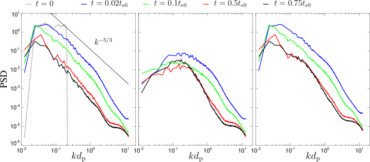
Figure 2.— 1-D PSD of the (left) perpendicular $B_{\perp}$, (middle) parallel $B_{\|}$, and total (right) $B$ fluctuating magnetic field, normalized to $B_{0}^{2}d_{\mathrm{p}0}$, as functions of $k$ at different times. The dotted line shows the initial spectrum and the thin solid line shows a dependence $\propto k^{-5/3}$ for comparison.

Figure 3 presents 1-D PSD of the proton velocity field $u_{\perp}$ (left) and $u_{\|}$ (middle), and the proton (number) density (right) as functions of $k$ at $t=0$ (dotted line), $t=0.02t_{e0}$ (blue) $t=0.1t_{e0}$ (green), $t=0.5t_{e0}$ (red), and $t=0.75t_{e0}$ (black solid). The power spectra of $u_{\perp}$ exhibit an exponential-like behavior from large to sub-ion scales (alternatively, this may be a smooth transition between two power-law like dependencies but it’s hard to distinguish between the two for the relatively short range of wave vectors); for $kd_{\mathrm{p}}\gtrsim 2$ the spectra are dominated by the numerical noise due to the finite number of particles per cell (Franci et al., 2015a). The power spectra of $u_{\|}$ are relatively flat at large scales and below about $k\rho_{\mathrm{p}}$ they exhibit rather power-law like properties (with a slope about $-3$) and again, for $kd_{\mathrm{p}}\gtrsim 2$ the spectra are dominated by the numerical noise. The amplitudes of $u_{\perp}$ and $u_{\|}$ decreases with time but at later times they are roughly constant. The power spectra of $\delta n$ at early times have properties of two power laws (but the ranges of wave vectors are too short to be sure) with a relatively thin transition, and their amplitude decreases in the time. At later times the amplitude of density fluctuations increases and has a property of a wide spectral peak with the maximum around $kd_{\mathrm{p}}\sim 10^{-1}$. As in the case of the velocity fluctuations the density spectra are dominated by the numerical noise for $kd_{\mathrm{p}}\gtrsim 2$.

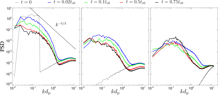
Figure 3.— 1-D PSD of the fluctuating proton velocity field $u_{\perp}$ (left), $u_{\|}$ (middle), normalized to $v_{A0}^{2}d_{\mathrm{p}0}$, and of the density fluctuations $\delta n$ (right), normalized to $\langle n\rangle^{2}d_{\mathrm{p}0}$, as functions of $k$ at different times. The dotted line shows the initial spectra and the thin solid line shows a dependence $\propto k^{-5/3}$ for comparison.

The generation of compressible fluctuations affects some ratios used to analyze properties of turbulent fluctuations. Figure 4 shows (left) the ratio between perpendicular electric and magnetic fluctuations, (middle) the ratio between squared amplitudes of the parallel and the total magnetic fluctuations, and (right) the ratio between squared amplitudes of density and perpendicular magnetic fluctuations as functions of $k$ at different times. The simulation results show that the transverse fluctuations are not strongly affected by the presence of the compressible fluctuations (cf., Bale et al., 2005; Matteini et al., 2017) whereas, unsurprisingly, the compressible ratios $\delta n^{2}/\delta B_{\perp}^{2}$ and $\delta B_{\|}^{2}/\delta B^{2}$ are strongly affected (cf., Kiyani et al., 2013; Franci et al., 2015b).

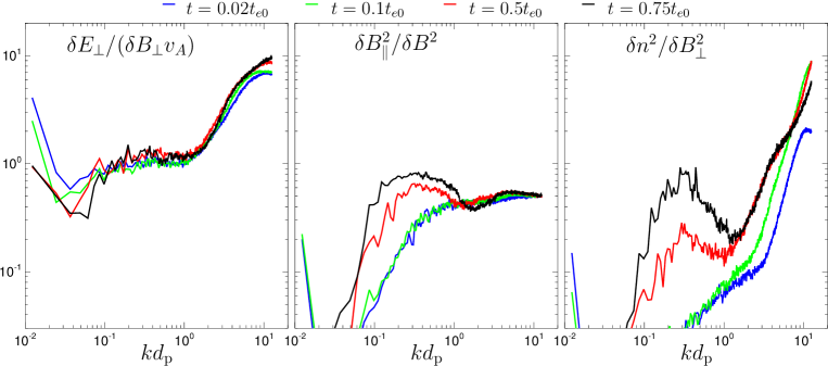
Figure 4.— (left) The ratio between perpendicular electric and magnetic fluctuations, (middle) the ratio between squared amplitudes of the parallel and the total magnetic fluctuations, and (right) the ratio between squared amplitudes of density and perpendicular magnetic fluctuations as functions of $k$ at different times.

The spatial properties of the magnetic fluctuations are shown in Figure 5 where $\delta B_{\perp}$ and $\delta B_{z}$ are displayed as functions of $x$ and $y$ at different times: (top) $t=0.1t_{e0}$, (middle) $t=0.5t_{e0}$, and (bottom) $t=0.75t_{e0}$. Only a part of the simulation box is shown; note that the radial, $y$ size of the simulation box normalized to $d_{\mathrm{p}}$ decreases in time as $d_{\mathrm{p}}\propto R$ (see the animation corresponding to Figure 5). The slow expansion introduces an anisotropy with respect to the radial direction (Dong et al., 2014; Verdini & Grappin, 2015, 2016); this happens mainly on the large scales, the turbulent characteristic time scales on the scales resolved in the present simulation are much faster then the expansion time so that no clear anisotropy is observed in our simulation (cf., Vech & Chen, 2016). Figure 5 shows the turbulent field of magnetic islands/vortices in $\delta B_{\perp}$ and formation of localized magnetic enhancements/humps in the compressible magnetic component $\delta B_{z}$ that are evident at later times but weak signatures of these structures are already seen at $t=0.1t_{e0}$. The compressible structures are likely the expected mirror mode structures, a more detailed analysis indicates that these structures are standing in the local plasma frame (they are moving with the turbulent plasma flow, see the animation corresponding to Figure 5).

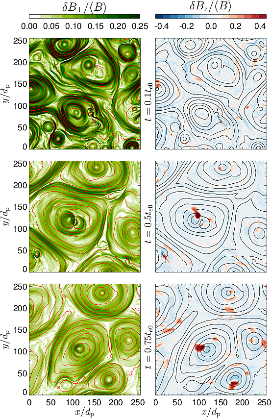
Figure 5.— Color scale plots of (left) $\delta B_{\perp}$ and (right) $\delta B_{z}$ as functions of $x$ and $y$ for (top) $t=0.1t_{e0}$, (middle) $t=0.5t_{e0}$, and (bottom) $t=0.75t_{e0}$. The solid lines show selected (projected) magnetic field lines. Only a part of the simulation box is shown.

A detailed view of the spatial structure is displayed in Figure 6 showing 1-D cuts of $\delta B_{x}$, $\delta B_{y}$, $\delta B_{z}$ (all normalized to $\langle B\rangle$), and $\delta n$ (normalized to $\langle n\rangle$) as functions of $x$ at $y=110d_{\mathrm{p}}$ and $t=0.75t_{e0}$ (see Figure 5, bottom). $\delta B_{x}$ and $\delta B_{y}$ components of the fluctuating magnetic field have a complex structure, at around $x=110d_{\mathrm{p}}$ the cut passes a center of a relatively large magnetic vortex. Close to this center the compressible component $\delta B_{z}$ forms a magnetic hump with a strong amplitude $\delta B_{z}/\langle B\rangle\sim 0.5$. The magnetic enhancement is compensated by a density decrease; the magnetic hump/density hole structure is roughly at pressure balance.

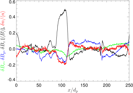
Figure 6.— Spatial profiles of $\delta B_{x}$, $\delta B_{y}$, $\delta B_{z}$ (all normalized to $\langle B\rangle$), and $\delta n$ (normalized to $\langle n\rangle$) as functions of $x$ at $y=110d_{\mathrm{p}}$ for $t=0.75t_{e0}$. (see Figure 5, bottom).

The pressure-balanced magnetic humps are characterized by an anti-correlation between the magnetic field component $B_{z}$ and the proton density and the distribution of $B_{z}$ values has a skewed distribution with a positive skewness (Génot et al., 2009). Figure 7 shows the evolution of the correlation between $n$ and $B_{z}$ and the skewness of $B_{z}$, $\mathcal{S}(B_{z})$, calculated over the whole box, as functions of time. Initially in the simulation, $B_{z}$ and $n$ are correlated indicating fast mode-like properties. $B_{z}$ and $n$ rapidly become anti-correlated suggesting a slow mode-like behavior; a similar evolution is seen in standard 2-D hybrid simulations of Franci et al. (2016). At later times the anti-correlation is strengthened by development of mirror structures. The skewness $\mathcal{S}(B_{z})$ starts around zero, then steadily increases, and for $t\gtrsim 0.3t_{e0}$ saturates around $3$. It is interesting to note that a similar analysis applied to the results from standard 2-D hybrid simulations of Franci et al. (2016) shows that the skewness $\mathcal{S}(B_{z})$ is negative in a well-developed turbulent cascade starting from an isotropic proton distribution for a wide range of betas.

Figure 7.— Time evolution of different quantities: (top) the correlation between the compressible component $B_{z}$ and the proton number density $n_{\mathrm{p}}$ and (bottom) of the skewness of $B_{z}$, $\mathcal{S}(B_{z})$, as functions of time.

Figure 8 shows the simulation results $(\beta_{\mathrm{p}\|},T_{\mathrm{p}\perp}/T_{\mathrm{p}\|})$ at different times, (top) $t=0.1t_{e0}$, (middle) $t=0.5t_{e0}$, and (bottom) $t=0.75t_{e0}$. The shades of blue display the distribution of the local (grid) values whereas the solid circles indicate the values averaged over the simulation box. The empty circle denotes the initial condition and the solid line gives the evolution of the averaged values. During the evolution, a large spread of local values develops in the space $(\beta_{\mathrm{p}\|},T_{\mathrm{p}\perp}/T_{\mathrm{p}\|})$ (cf., Servidio et al., 2015; Hellinger et al., 2015). The expansion drives the system towards more unstable situations but the development of mirror modes reduces the anisotropy and tends to stabilize the system. A small subset of local values in the space $(\beta_{\mathrm{p}\|},T_{\mathrm{p}\perp}/T_{\mathrm{p}\|})$ have smaller values of the maximum growth rates (compared to the average value); the places where the mirror instability is weakened appear in the vicinity of the mirror structures. The reduction of the local proton temperature anisotropy is mainly governed by the enhanced magnetic field that leads to higher proton perpendicular temperatures, the magnetic moment of protons is varying only weakly (cf., Schekochihin et al., 2008). The variation of the magnetic field is not, however, the only saturation mechanism. Figure 9 shows the proton velocity distribution $f$ (averaged over the simulation box) as a function of parallel and perpendicular velocities $v_{\|}$ and $v_{\perp}$ (with respect to the local magnetic field) at different times: (top) $t=0.1t_{e0}$, (middle) $t=0.5t_{e0}$, and (bottom) $t=0.75t_{e0}$. The averaged proton distribution function exhibit a clear flattening around $v_{\|}=0$, i.e., $\partial f/\partial v_{\|}\sim 0$ for $v_{\perp}\gtrsim 2v_{A}$. This is compatible with the quasi-linear diffusion of protons through the Landau (transit time) resonance (Califano et al., 2008; Hellinger et al., 2009).

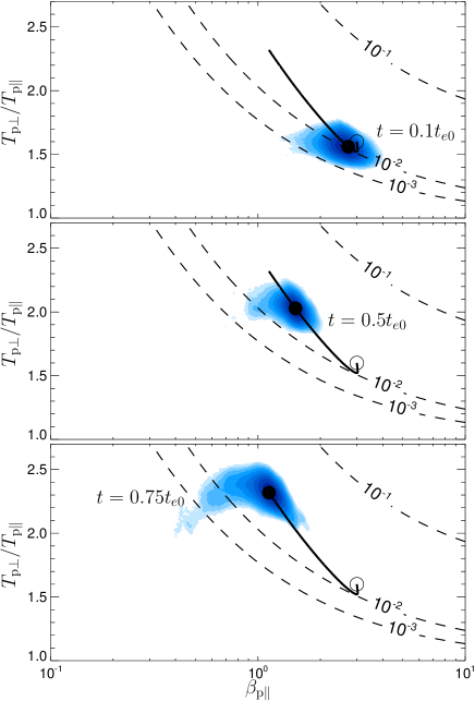
Figure 8.— Simulated data distribution in the plane $(\beta_{\mathrm{p}\|},T_{\mathrm{p}\perp}/T_{\mathrm{p}\|})$ at different times. The empty circles give the initial condition whereas the solid circles denote the average values and the solid lines show their evolution. The dashed contours show the maximum growth rate $\gamma_{max}$ (in units of $\Omega_{\mathrm{p}}$) of the mirror instability as a function of $\beta_{\mathrm{p}\|}$ and $T_{\mathrm{p}\perp}/T_{\mathrm{p}\|}$ in the corresponding plasma with bi-Maxwellian protons.

Both the linear and nonlinear properties of the mirror instability in the nonlinear reductive perturbative model (Kuznetsov et al., 2007a, b; Califano et al., 2008) are sensitive to the details of the proton distribution function in the resonant region $v_{\|}\sim 0$. The flattening observed in the simulation likely modifies the nonlinear properties and leads to generation of magnetic humps (instead of holes that are expected for bi-Maxwellian velocity distribution functions (Hellinger et al., 2009)) in agreement with the simulation results.

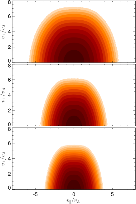
Figure 9.— Average proton velocity distribution function $f$ as a function of parallel and perpendicular velocities $v_{\|}$ and $v_{\perp}$ (with respect to the local magnetic field) for (top) $t=0.1t_{e0}$, (middle) $t=0.5t_{e0}$, and (bottom) $t=0.75t_{e0}$.

IV. Discussion

The presented 2-D hybrid simulation of plasma turbulence with the expansion forcing demonstrates that mirror instability may coexist with the fully developed (strong) turbulence and generate compressible, nonpropagating pressure-balanced magnetic structures with amplitudes comparable to or even greater than those of the ambient turbulent fluctuations. The compressible component of the magnetic field $B_{\|}$ becomes at later times important on scales comparable to and larger than the typical proton scales and this affects the total power spectra of $B$ around the transition between large MHD and sub-ion scales (cf., Lion et al., 2016), as well as different compressibility ratios. The mirror structures reduce locally the temperature anisotropy through a fluid mechanism (generation of enhanced magnetic field that increases the proton perpendicular temperature) and through a quasilinear-like proton scattering via the Landau (transit time) resonance. The role of particle trapping in the present case is unclear (Rincon et al., 2015).

The dominant, compressible magnetic component of the mirror structures only weakly interacts with the incompressible turbulent Alfvénic fluctuations through the main fluid nonlinearities. On the other hand, the minor, transverse component of mirror fluctuations have a vortex like properties around the compressible structures (Passot et al., 2014) and likely couples directly to the turbulent plasma motions (the present simulation indicates presence of such vortical structures). Further work is necessary to understand the interaction between turbulence and the mirror instability.

In this paper we drive the temperature anisotropy by the expansion with the transverse magnetic field. We expect a similar evolution for other driving forces that generate the perpendicular proton/ion temperature anisotropy (Kunz et al., 2014). Our work is relevant mainly for high beta plasmas where the mirror instability is dominant; for low and moderate beta plasmas the ion cyclotron instability is prevalent (Gary, 1992; Lacombe & Belmont, 1995). The nonlinear competition between these instabilities is a nontrivial problem even in a homogeneous system and generally requires fully three-dimensional (3-D) simulations (Shoji et al., 2009). In the present case, both turbulence and the 2-D geometry constraints strongly affect the dynamics of the mirror instability. In the 2-D simulation box we have only limited access to oblique modes; however, the mirror instability appear at strongly oblique angles with respect to the ambient magnetic field (in a homogeneous plasma system) near threshold (Hellinger, 2007). The 2-D geometry is likely a smaller problem for the mirror instability compared to the oblique fire hose (cf., Hellinger et al., 2015) but, in any case, 3-D simulations are needed to investigate the interplay between turbulence and instabilities. We expect that 3-D simulations with turbulent fluctuations will exhibit an evolution similar to the 2-D simulation of Trávníček et al. (2007) modified by turbulence; this will be subject of future work. Despite the limitations, the present simulation results confirm that the mirror instability is a viable mechanism that can generate magnetic pressure-balanced structures in turbulent astrophysical plasmas.

References

- Bale et al. (2005) Bale, S. D., Balikhin, M. A., Horbury, T. S., et al. 2005, Space Sci. Rev., 118, 161
- Califano et al. (2008) Califano, F., Hellinger, P., Kuznetsov, E., et al. 2008, J. Geophys. Res., 113, A08219, doi:10.1029/2007JA012898
- Dong et al. (2014) Dong, Y., Verdini, A., & Grappin, R. 2014, ApJ, 793, 118, doi:10.1088/0004-637X/793/2/118
- Enríquez-Rivera et al. (2013) Enríquez-Rivera, O., Blanco-Cano, X., Russell, C. T., et al. 2013, J. Geophys. Res., 118, 17, doi:10.1029/2012JA018233
- Franci et al. (2015a) Franci, L., Landi, S., Matteini, L., Verdini, A., & Hellinger, P. 2015a, ApJ, 812, 21, doi:10.1088/0004-637X/812/1/21
- Franci et al. (2016) —. 2016, ApJ, 833, 91, doi:10.3847/1538-4357/833/1/91
- Franci et al. (2015b) Franci, L., Verdini, A., Matteini, L., Landi, S., & Hellinger, P. 2015b, ApJL, 804, L39, doi:10.1088/2041-8205/804/2/L39
- Gary (1992) Gary, S. P. 1992, J. Geophys. Res., 97, 8519
- Génot et al. (2011) Génot, V., Broussillou, L., Budnik, E., et al. 2011, Ann. Geophys., 29, 1849
- Génot et al. (2009) Génot, V., Budnik, E., Hellinger, P., et al. 2009, Ann. Geophys., 27, 601
- Hasegawa (1969) Hasegawa, A. 1969, Phys. Fluids, 12, 2642
- Hellinger (2007) Hellinger, P. 2007, Phys. Plasmas, 14, 082105
- Hellinger (2008) —. 2008, Phys. Plasmas, 15, 054502
- Hellinger (2017) —. 2017, J. Plasma Phys., 83, 705830105, doi:10.1017/S0022377817000071
- Hellinger et al. (2009) Hellinger, P., Kuznetsov, E. A., Passot, T., Sulem, P. L., & Trávníček, P. M. 2009, Geophys. Res. Lett., 36, L06103, doi:10.1029/2008GL036805
- Hellinger et al. (2015) Hellinger, P., Matteini, L., Landi, S., et al. 2015, ApJL, 811, L32, doi:10.1088/2041-8205/811/2/L32
- Hellinger & Trávníček (2005) Hellinger, P., & Trávníček, P. 2005, J. Geophys. Res., 110, A04210, doi:10.1029/2004JA010687
- Herčík et al. (2013) Herčík, D., Trávníček, P. M., Johnson, J. R., Kim, E.-H., & Hellinger, P. 2013, J. Geophys. Res., 118, 405, doi:10.1029/2012JA018083
- Kiyani et al. (2013) Kiyani, K. H., Chapman, S. C., Sahraoui, F., et al. 2013, ApJ, 763, 10, doi:10.1088/0004-637X/763/1/10
- Kunz et al. (2014) Kunz, M. W., Schekochihin, A. A., & Stone, J. M. 2014, Phys. Rev. Lett., 112, 205003, doi:10.1103/PhysRevLett.112.205003
- Kuznetsov et al. (2007a) Kuznetsov, E. A., Passot, T., & Sulem, P. 2007a, JETP Lett., 86, 637, doi:10.1134/S0021364007220055
- Kuznetsov et al. (2007b) Kuznetsov, E. A., Passot, T., & Sulem, P.-L. 2007b, Phys. Rev. Lett., 98, 235003, doi:10.1103/PhysRevLett.98.235003
- Lacombe & Belmont (1995) Lacombe, C., & Belmont, G. 1995, Adv. Space Res., 15, 329
- Lion et al. (2016) Lion, S., Alexandrova, O., & Zaslavsky, A. 2016, ApJ, 824, 47, doi:10.3847/0004-637X/824/1/47
- Matteini et al. (2017) Matteini, L., Alexandrova, O., Chen, C. H. K., & Lacombe, C. 2017, MNRAS, 466, 945, doi:10.1093/mnras/stw3163
- Matteini et al. (2012) Matteini, L., Hellinger, P., Landi, S., Trávníček, P. M., & Velli, M. 2012, Space Sci. Rev., 172, 373, doi:10.1007/s11214-011-9774-z
- Matthews (1994) Matthews, A. 1994, J. Comput. Phys., 112, 102
- Mininni & Pouquet (2009) Mininni, P. D., & Pouquet, A. 2009, Phys. Rev. E, 80, 025401, doi:10.1103/PhysRevE.80.025401
- Pantellini et al. (1995) Pantellini, F. G. E., Burgers, D., & Schwartz, S. J. 1995, Adv. Space Res., 15, 341
- Passot et al. (2014) Passot, T., Henri, P., Laveder, D., & Sulem, P.-L. 2014, Eur. Phys. J. D, 68, 207, doi:10.1140/epjd/e2014-50160-1
- Passot et al. (2006) Passot, T., Ruban, V., & Sulem, P. L. 2006, Phys. Plasmas, 13, 102310, doi:10.1063/1.2356485
- Rincon et al. (2015) Rincon, F., Schekochihin, A. A., & Cowley, S. C. 2015, MNRAS, 447, L45, doi:10.1093/mnrasl/slu179
- Schekochihin et al. (2008) Schekochihin, A. A., Cowley, S. C., Kulsrud, R. M., Rosin, M. S., & Heinemann, T. 2008, Phys. Rev. Lett., 100, 081301, doi:10.1103/PhysRevLett.100.081301
- Servidio et al. (2015) Servidio, S., Valentini, F., Perrone, D., et al. 2015, J. Plasma Phys., 81, 325810107, doi:10.1017/S0022377814000841
- Shapiro & Shevchenko (1964) Shapiro, V. D., & Shevchenko, V. I. 1964, Sov. Phys. JETP, Engl. Transl., 18, 1109
- Shoji et al. (2009) Shoji, M., Omura, Y., Tsurutani, B. T., Verkhoglyadova, O. P., & Lembege, B. 2009, J. Geophys. Res., 114, A10203, doi:10.1029/2008JA014038
- Soucek et al. (2008) Soucek, J., Lucek, E., & Dandouras, I. 2008, J. Geophys. Res., 113, A04203, doi:10.1029/2007JA012649
- Southwood & Kivelson (1993) Southwood, D. J., & Kivelson, M. G. 1993, J. Geophys. Res., 98, 9181
- Stevens & Kasper (2007) Stevens, M. L., & Kasper, J. C. 2007, J. Geophys. Res., 112, A05109, doi:10.1029/2006JA012116
- Trávníček et al. (2007) Trávníček, P., Hellinger, P., Taylor, M. G. G. T., et al. 2007, Geophys. Res. Lett., 34, L15104, doi:10.1029/2007GL029728
- Tsurutani et al. (2011) Tsurutani, B. T., Lakhina, G. S., Verkhoglyadova, O. P., et al. 2011, J. Geophys. Res., 116, A02103, doi:10.1029/2010JA015913
- Vech & Chen (2016) Vech, D., & Chen, C. H. K. 2016, ApJL, 832, L16, doi:10.3847/2041-8205/832/1/L16
- Vedenov & Sagdeev (1958) Vedenov, A. A., & Sagdeev, R. Z. 1958, in Plasma Physics and the Problem of Controlled Thermonuclear Reactions, Vol. 3 (New York: Pergamon), 332–339
- Verdini & Grappin (2015) Verdini, A., & Grappin, R. 2015, ApJL, 808, L34, doi:10.1088/2041-8205/808/2/L34
- Verdini & Grappin (2016) —. 2016, ApJ, 831, 179, doi:10.3847/0004-637X/831/2/179
- Winterhalter et al. (1995) Winterhalter, D., Neugebauer, M., Goldstein, B. E., et al. 1995, Space Sci. Rev., 72, 201