Natural Time Analysis of Seismicity in California: The epicenter of an impending mainshock

Abstract

Upon employing the analysis in a new time domain, termed natural time, it has been recently demonstrated that a remarkable change of seismicity emerges before major mainshocks in California. What constitutes this change is that the fluctuations of the order parameter of seismicity exhibit a clearly detectable minimum. This is identified by using a natural time window sliding event by event through the time series of the earthquakes in a wide area and comprising a number of events that would occur on the average within a few months or so. Here, we suggest a method to estimate the epicentral area of an impending mainshock by an additional study of this minimum using an area window sliding through the wide area. We find that when this area window surrounds (or is adjacent to) the future epicentral area, the minimum of the order parameter fluctuations in this area appears at a date very close to the one at which the minimum is observed in the wide area. The method is applied here to major mainshocks that occurred in California during the recent decades including the strongest one, i.e., the 1992 Landers earthquake.

It may be considered (e.g. refs. Turcotte, 1997; Holliday et al., 2006) that earthquakes are non-equilibrium critical phenomena. Their complex correlations in time, space and magnitude $M$ have been investigated by various procedures (e.g., see refs. Huang (2008); Telesca (2010); Lennartz et al. (2011); Lippiello et al. (2012); Tenenbaum et al. (2012)) including a very recent development Tenenbaum et al. (2012) of the complex networks approach. In this study, we employ the analysis in a new time domain, termed natural timeVarotsos et al. (2002a, b); Tanaka et al. (2004), $\chi$, since it allows us to identifyVarotsos et al. (2011a) when a system approaches a critical point (for a review see ref. Varotsos et al., 2011b).

Seismic Electric Signals (SES) are low frequency ($\leq 1$Hz) electric signals Varotsos and Alexopoulos (1984) preceding earthquakes. They are emitted from the future focal region probably through the following mechanism Varotsos et al. (2013): When in the focal region the stress reaches a critical value $\sigma_{cr}$, a cooperative orientation of the electric dipoles (that have been formed due to defectsVarotsos and Alexopoulos (1978); Varotsos (1980); Varotsos et al. (1982); Varotsos and Alexopoulos (1982); Varotsos (2008)) occurs, which leads to the emission of a transient electric signal that constitutes an SES. Several such signals within a short time are called SES activity Varotsos et al. (1996); Varotsos et al. (2003a, b). By combining the SES physical properties, the epicenter and the magnitude of the impending mainshock can be determinedVarotsos et al. (1996). Furthermore, by making use of the small earthquakes subsequent to the initiation of an SES activity and analyzing them in natural time (see below), the occurrence time of an impending mainshock can be identified as follows: We compute the value of the order parameter $\kappa_{1}$ of seismicity (see below) and then findVarotsos et al. (2006); Sarlis et al. (2008) that a mainshock occurs in a few days to one week after the $\kappa_{1}$ value approaches 0.070. By applying this procedure, several successful predictions have been issued Varotsos et al. (2011b) in Greece.

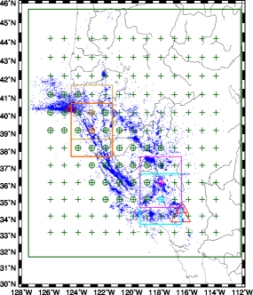
Figure 1: (color online) Map of the earthquake epicenters (blue dots) in the wide area (green rectangle): $N_{31.7}^{45.7}W_{127.5}^{112.1}$ ($M\geq 2.5$) during 1 January 1979 - 1 January 2004 as reported by NCEDC. The major mainshocks in California discussed in this paper are shown with red triangles and the neighboring rectangles depict their tentative epicentral area estimated by means of the procedure described in the text. The 156 green plus symbols depict the locations of the area window of size $3^{o}\times 3^{o}$ sliding through the wide area $14^{o}\times 15.4^{o}$ out of which 38 are encircled in order to show that they contain at least 24 events occurring on average in three months.

The challenging question raises, however, what can we do when geoelectrical data are lacking which was the case before the occurrence of the most strong earthquakes (EQs) worldwide during the recent decades. It is the main objective of this paper to attempt answering this question motivated by an important fact which has been recently reported Varotsos et al. (2013): The initiation of an SES activity is accompanied by a clearly detectable change in seismicity which constitutes an independent geophysical dataset of a different physical observable. In particular, by analyzing in natural time the time series of earthquakes, we found that the fluctuations of the order parameter of seismicity exhibited a clearly detectable minimum approximately at the time of the initiation of the SES activity. Furthermore, we showed Varotsos et al. (2013) that these two phenomena (SES activity, minimum of the order parameter fluctuations of seismicity) beyond their co-location in time they were also linked closely in space. Here, we take advantage of these recent findings and show the following: Since the natural time analysis of the seismic data alone can lead to the identification of the minimum of the fluctuations of the order parameter of seismicity that precedes a major EQ, an adequate study of the spatial distribution of those events resulting in this precursory minimum enables an estimate of the area in which the major EQ will occur. We shall present applications including the strongest EQ that occurred in California (see Fig. 1) during the last three decades. Analogous applications have been completed for major EQs in JapanSarlis et al. (2013, 2015).

I The procedure for the data analysis

We first briefly describe the natural time analysis of seismicity Varotsos et al. (2011b); Varotsos et al. (2005). In a time series comprising $N$ earthquakes, the natural time $\chi_{k}=k/N$ serves as an index for the occurrence of the $k$-th earthquake. In natural time analysis the pair $(\chi_{k},Q_{k})$ is studied, where $Q_{k}$ is the energy released during the $k$-th earthquake of magnitude $M_{k}$. Alternatively, one may study the pair $(\chi_{k},p_{k})$, where $p_{k}={Q_{k}}/{\sum_{n=1}^{N}Q_{n}}$ is the normalized energy released during the $k$-th earthquake, and $Q_{k}$ -and hence $p_{k}$- is estimated through the relation Kanamori (1978) $Q_{k}\propto 10^{1.5M_{k}}$. The variance of $\chi$ weighted for $p_{k}$, designated by $\kappa_{1}$, is given by Varotsos et al. (2002a, 2011b, 2003b, 2003a); Varotsos et al. (2005)

$$\kappa_{1}=\sum_{k=1}^{N}p_{k}(\chi_{k})^{2}-\left(\sum_{k=1}^{N}p_{k}\chi_{k}\right)^{2}$$ (1)

This quantity can be also considered as an order parameter for seismicityVarotsos et al. (2005); Varotsos et al. (2011b).

In order to study the fluctuations of $\kappa_{1}$, we apply the following procedure Varotsos et al. (2011b). Taking an excerpt of a seismic catalog comprising $W(\geq 100)$ successive events, we start from the first EQ and calculate the first 35 $\kappa_{1}$ values for 6 to 40 consecutive EQs (cf. the upper limit of this number does not markedly influence the results Varotsos et al. (2006)). Then we proceed to the second EQ, and calculate again 35 values of $\kappa_{1}$ using the 7^th to the 41^st event. Scanning, event by event, the whole excerpt of $W$ earthquakes, we calculate the average value $\mu(\kappa_{1})$ and the standard deviation $\sigma(\kappa_{1})$ of the $\kappa_{1}$ values. The quantity

$$\beta\equiv\sigma(\kappa_{1})/\mu(\kappa_{1})$$ (2)

is definedSarlis et al. (2010) as the variability $\beta$ of $\kappa_{1}$ for this excerpt of length $W$. Usually we are interested on what happens to the $\beta$ value until just before the occurrence of each EQ, $e_{i}$, in the seismic catalog. To achieve this goal, we calculate first the $\kappa_{1}$ values using the previous 6 to 40 (or 6 to $W$)Sarlis et al. (2013, 2015) consecutive EQs. These 35 $\kappa_{1}$ values are associated with the EQ $e_{i}$, but we clarify that the EQ $e_{i}$ has not been employed for their calculation. The $\beta$ value -corresponding to the EQ $e_{i}$- for a natural time window length $W$ is computed using all the ($35\times W$) $\kappa_{1}$ values associated with the EQs $e_{i-W+1}$ to $e_{i}$. The resulting value is denoted by $\beta_{W}$, where the subscript $W$ shows the natural time window length, and the corresponding minimum is designated by $\beta_{W,min}$.

We now summarize a few important points that emerged in our earlier studiesVarotsos et al. (2005, 2006), reviewed also in chapter 6 of ref. Varotsos et al., 2011b, when analyzing in natural time the long term seismicity in wide areas. By using a natural time window comprising 6 to 40 consecutive events sliding through an earthquake catalog, the computed $\kappa_{1}$ values lead to the construction of the probability density function (pdf) P($\kappa_{1}$) of a wide area. The scaled distribution $\sigma(\kappa_{1})$ P($\kappa_{1}$) plotted versus ($\mu(\kappa_{1})-\kappa_{1}/\sigma(\kappa_{1})$) of this area collapses on the same curve with the ones deduced from different wide areas. For example, the curve obtained from the area $N_{25}^{46}E_{125}^{146}$ in Japan using the JMA catalog, and the area $N_{32}^{37}W_{114}^{122}$ in California using the southern California earthquake catalog (SCEC) Varotsos et al. (2005). It has been also found that this universal curve of long term seismicity exhibits strikingly similar features with the corresponding scaled distribution curves of the order parameter fluctuations in other -nonequilibrium or equilibrium- critical systemsBramwell et al. (1998, 2001); Zheng and Trimper (2001); Zheng (2003); Clusel et al. (2004) including the dataAegerter et al. (2004); Lőrincz and Wijngaarden (2007) we analyzedSarlis et al. (2011) for the case of self organized criticalityBak et al. (1987). This similarity was focused on the existence of a common “exponential tail” (which has in fact a double exponential form) reflecting non-Gaussian (large, but rare) fluctuations.

II The data analyzed

In this study we present examples of major EQs that occurred in California. We used the United States Geological Survey Northern California Seismic Network catalog available from the Northern California Earthquake Data Center, at the http address: www.ncedc.org/ncedc/catalog-search.html, hereafter called NCEDC. The earthquake magnitudes reported in this catalog are hereafter labelled with $M$. We considered all earthquakes with $M\geq 2.5$ reported by NCEDC, within the area ${\rm N}_{31.7}^{45.7}{\rm W}_{127.5}^{112.1}$ (the green rectangle in Fig. 1). We have on average $\sim 10^{2}$ EQs per month since 31832 earthquakes occurred for the 25 year period from 1 January 1979 to 1 January 2004.

Following ref. Varotsos et al., 2012, we focus hereafter on the natural time window length $W=$300, which is compatible with the fact that the lead time of SES activities is around a few months (i.e., from 21 days to an upper limit of around 5 months, e.g., see ref. Varotsos et al., 2011b). By analyzing in natural time the aforementioned NCEDC data, we recently identified Varotsos et al. (2012), for $W$=300 events, the dates of the minima $\beta_{W,min}$ as being 1 to 5 months before four out of the five mainshocks with $M\geq 7.0$ that occurred within the wide area $N_{31.7}^{45.7}W_{127.5}^{112.1}$ during the 25 year period 1 January 1979 to 1 January 2004 in California. For the two examples of the $M$7.4 Landers EQ on 28 June 1992 and the $M$7.0 Hector Mine EQ on 16 October 1999 that will be treated below, the dates of the precursory minima $\beta_{300,min}$ were reported to be 28 January 1992 and 14 May 1999, respectively.

III The method proposed to estimate the epicentral area of an impending mainshock

Briefly, the method proposed in based on the following main aspect: We argue that a minimum should be observed almost simultaneously in the order parameter fluctuations of the seismicity within both the wide area and the epicentral area of the impending mainshock. This stems from our findings in ref. Varotsos et al., 2013 where we identified the appearance of a $\beta_{W,min}$ (at scales $W$=100 to $W$=400) in the seismicity within the wide area $N_{25}^{46}E_{125}^{146}$, i.e., $21^{o}\times 21^{o}$, in Japan around the date (i.e., on 26 April 2000) of the initiation of the SES activity recordedUyeda et al. (2002) at Niijima Island -in the vicinity of which a major seismic swarm started 2 months later with a $M$6.5 EQ on 1 July 2000. Moreover, it was found that in areas surrounding Niijima Island the variability $\beta$ of the seismicity exhibited a minimum almost at the same date, i.e., around 26 April. Hence, in the light of the above findings, the method to estimate the epicentral area of an impending mainshock -when no information for the recording of an SES activity is available- should consist of the following steps:

First step: We start the investigation from the natural time analysis of the seismicity in a wide area, for example $N_{31.7}^{45.7}W_{127.5}^{112.1}$ (i.e., $14^{o}\times 15.4^{o}$) in California. By considering a sliding natural time window comprising a number of events that would occur in a few months (e.g., we may adopt, as in ref. Varotsos et al., 2012, $W$=300 events for the aforementioned wide area in California), we search for a minimum in the $\beta$ variability.

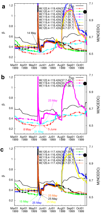
Figure 2: (color online) Results for the $M$7.0 Hector Mine EQ in California on 16 October 1999. (a) The variability $\beta$ of the seismicity versus the conventional time for a natural time window length $W$ comprising a number of events that would occur in three months: The thick black curve minimizing on 14 May 1999 corresponds to the wide area $N_{31.7}^{45.7}W_{127.5}^{112.1}$. The other eight curves correspond to those areas -out of the 38 encircled ones in Fig. 1- resulting in $\beta$ minima which occur at dates close to that of the $\beta_{300}$ minimum of the wide area. These dates for the lower three minima are marked in (b) and for the remaining five minima in (c). (b): After discarding the red curve (see the text), the cyan curve exhibits the lowest minimum on 21 May 1999. It corresponds to the area $N_{33.7}^{36.7}W_{119.4}^{116.4}$ shown in Fig. 1 by the cyan rectangle along with the Hector Mine EQ epicenter marked with the neighboring red triangle (the smaller). The EQs with $M\geq 6.4$ (right scale) are shown with vertical bars ending at solid circles.

Second step: We investigate whether this minimum is a precursory one by examining whether it obeys the criteria mentioned in ref. Varotsos et al., 2012. This should necessarily include the Detrended Fluctuation Analysis (DFA)Peng et al. (1994) in order to investigate temporal correlations in the earthquake magnitude time series at the same natural time window length scale as the one mentioned above (cf. It has been shown Varotsos et al. (2014) that $\beta$ captures the correlations between the events). DFA has become the standard method when studying long-range correlated time series and can also be applied to real world non-stationary signals Hu et al. (2001); Chen et al. (2002, 2005); Ma et al. (2010); Xu et al. (2011).

Third step: We search for the epicentral area of the impending mainshock by using an area window of an appreciably smaller size, e.g., $3^{o}\times 3^{o}$ for the cases studied in California, sliding (with steps of $1^{o}$ in longitude and/or $1^{o}$ in latitude, see the green plus symbols in Fig. 1) through the wide area. For each location of the sliding area window, we repeat the analysis as in the wide area in order to determine the date of $\beta_{W,min}$. Note that, if in the aforementioned wide area of California (in which, as mentioned, occur on average 100 events/month) we used $W$=300 events, we should consider as $W$ in each location of the sliding area window the corresponding number of the events that would occur on average within three months. This reflects that we cannot select an area window of arbitrarily smaller size in view of the following limitation: In order to identify the date of the occurrence of the minimum of $\beta$ in an area window size with an uncertainty of around a few days, we must have at least on the average 2 events per week, i.e., at least 24 events for an almost three month period (12 weeks). Among these locations of the sliding area window investigated, we select the one(s) which led to a $\beta_{W,min}$ date which almost coincides with the date at which the $\beta_{300,min}$ value was observed in the wide area. In practice, the former date differs from the latter usually by no more than a few days up to around 10 days, or so. This way we usually find an area surrounding the future epicenter, as it results from the examples presented in the following two Sections, which refer to major EQs that occurred in California.

Since a major EQ occurs, as mentioned, 1 to 5 months after the appearance of $\beta_{300,min}$ in the wide area Varotsos et al. (2012), the applicability of the method proposed here becomes more clear when a single major mainshock occurs within a five month period. Such an example, is the case of the $M$7.0 Hector Mine EQ in California in 1999. Furthermore, in a later Section, we shall present a case in which two major mainshocks occurred inside the wide area within 5 months. This is the case of the $M$7.4 Landers EQ on 28 June 1992 that was preceded by the $M$6.7 ($M_{s}$7.1, e.g. see ref. Tanioka et al., 1995) Cape Mendocino EQ on 25 April 1992. As we shall see later, it is strikingly interesting that in the latter case the method identifies two different epicentral areas as it should.

We clarify that in the next two Sections, we solely focus on the third step of the method since the first two steps -referring to the identification in the wide area of the dates of the minima $\beta_{300,min}$ for major EQs in California and their distinction from the non precursory minima- have been already accomplished, as mentioned, in ref. Varotsos et al., 2012.

To summarize: For the analysis of the examples presented below for California, we used the wide area $N_{31.7}^{45.7}W_{127.5}^{112.1}$ as in ref.Varotsos et al. (2012), and a sliding area window size $3^{o}\times 3^{o}$ (with step $1^{o}$) resulting in 156 areas (see the plus symbols in Fig. 1) out of which 38 areas (encircled in Fig. 1) had at least 24 events on average per three months. Hence, the investigation of the examples below in California was made by analyzing the seismic data occurring in these 38 areas.

IV Results concerning the $M$7.0 Hector Mine EQ on 16 October 1999 at $34.60^{o}$N $116.34^{o}$W in California

The thick black curve in Fig. 2a depicts the variability $\beta$ versus the conventional time when a natural time window length $W$=300 events is sliding through the wide area $N_{31.7}^{45.7}W_{127.5}^{112.1}$. A clear minimum of $\beta$ is observed on 14 May 1999, as marked in the figure. The subsequent analysis of the 38 areas -out of the 156 depicted in Fig. 1- resulting from the locations of the sliding window of size $3^{o}\times 3^{o}$ lead to 38 curves. Eight of these curves, depicted in Fig. 2a, were identified to exhibit a $\beta$ minimum with dates within 10 days, or so, from the aforementioned date on 14 May 1999 obtained from the wide area. These dates are now marked, for reader’s convenience, in two separate panels of this figure: In Fig. 2b -for the three lowest minima observed in Fig. 2a- and in Fig. 2c for the minima of the remaining five curves. A closer inspection of Fig. 2b shows that the red curve in the bottom (that is obtained from the area $N_{37.7}^{40.7}W_{122.4}^{119.4}$) has a plateau extending from 8 May until 5 June which in fact comes from the absence of the occurrence of any event in the area during this almost one month period. Thus, this curve should be discarded from further analysis since we cannot derive a definite conclusion on the existence or not of a minimum close to the aforementioned date 14 May 1999. Between the remaining two curves, the cyan has a minimum which is somewhat lower and occurs on 21 May 1999. It corresponds to the area $N_{33.7}^{36.7}W_{119.4}^{116.4}$ depicted with the cyan rectangle in Fig. 1 along with the epicenter of the Hector Mine EQ (the smaller red triangle) lying at $34.60^{o}$N $116.34^{o}$W. The epicenter is located just at the eastern edge of the area, see the cyan rectangle in Fig. 1. The other curve, i.e., the magenta in Fig.2b, corresponds to the area $N_{34.7}^{37.7}W_{119.4}^{116.4}$, see the magenta rectangle in Fig. 1, which is only $0.1^{o}$ far from the Hector Mine EQ epicenter. As for the five curves in Fig.2c they correspond to the areas $N_{34.7}^{37.7}W_{120.4}^{117.4}$, $N_{36.7}^{39.7}W_{121.4}^{118.4}$, $N_{35.7}^{38.7}W_{119.4}^{116.4}$, $N_{36.7}^{39.7}W_{119.4}^{116.4}$ and $N_{36.7}^{39.7}W_{120.4}^{117.4}$ lying at various distances (roughly between $1^{o}$ and $2.9^{o}$) from the Hector Mine EQ epicenter. None of these areas, is adjacent to the epicenter as the aforementioned one $N_{33.7}^{36.7}W_{119.4}^{116.4}$ which corresponds to the cyan curve exhibiting the lowest $\beta$ minimum in Figs. 2a,b.

Thus, in short, the cyan curve exhibiting a $\beta$ minimum on 21 May, i.e., around a week later from that (14 May) identified in the wide area (thick black curve), which happens to be the lowest one among the other curves showing also minima at neighboring dates, corresponds to an area whose eastern edge lies just at the Hector Mine EQ epicenter.

V Results concerning the $M$7.4 Landers EQ in California on 28 June 1992 at $34.19^{o}$N $116.46^{o}$W

This EQ, which is the largest moment magnitude ($M_{w}$) EQ that occurred in California since 1992, has been preceded by the $M$6.7 ($M_{s}$7.1) Cape Mendocino EQ on 25 April 1992 with an epicenter at $40.36^{o}$N $124.23^{o}$W (followed by two strong $M$6.45 and $M$6.6 aftershocks on 26 April 1992). Hence, Landers EQ and Cape Mendocino EQ occurred within almost 3 months being less than the maximum lead time between $\beta_{300,min}$ and the subsequent EQ which is around 5 months Varotsos et al. (2012). The complexity of this case might be the origin of the following fact: The variability of the seismicity versus the conventional time in the wide area $N_{31.7}^{45.7}W_{127.5}^{112.1}$, depicted in Fig. 3 with a thick black curve, although exhibited its lowest value on 28 January 1992 (marked in Fig. 3a, its minimum is in fact very broad (like a plateau) lasting for about 4 weeks, i.e., from 18 January to around 20 February, 1992. This must be carefully considered when the area window of $3^{o}\times 3^{o}$ is sliding (with step $1^{o}$) through the aforementioned wide area. We found that, among the 38 areas studied, eight of them led to $\beta$ minima with dates from 2 February to 19 February 1992, thus lying within the broad range mentioned above for the $\beta$ minimum of the wide area. The eight curves corresponding to these areas are plotted in Fig. 3a and can be classified into two types, which are depicted separately in Figs. 3b and 3c where we also mark the date of the minimum in each curve. First, in three of these curves shown with magenta squares, black triangles and cyan circles, which correspond to the areas $N_{33.7}^{36.7}W_{120.4}^{117.4}$, $N_{35.7}^{38.7}W_{120.4}^{117.4}$ and $N_{33.7}^{36.7}W_{119.4}^{116.4}$, a very sharp minimum appears on 19 February 1999, see Fig. 3b. An inspection of these three areas shows that the epicenter of Landers EQ in Fig. 1 (large red triangle) lies inside the latter area (depicted with a cyan rectangle in Fig. 1), $1^{o}$ to the east of the first area and around $1.8^{o}$ to the southeast of the second area. Second, the remaining five curves, see Fig. 3c, shown in orange circles, blue squares, red crosses, thin black line and green asterisks (starting from the curve with the lowest $\beta$ minimum), exhibit non-sharp minima on the following dates 2, 2, 2, 16 and 17 February, 1992, and correspond to the following five areas: $N_{37.7}^{40.7}W_{124.4}^{121.4}$, $N_{37.7}^{40.7}W_{123.4}^{120.4}$, $N_{36.7}^{39.7}W_{125.4}^{122.4}$, $N_{36.7}^{39.7}W_{124.4}^{121.4}$ and $N_{36.7}^{39.7}W_{123.4}^{120.4}$, respectively. The first area is depicted with the orange rectangle in Fig.1, where we see that the epicenter of the Cape Mendocino EQ marked by a red triangle -inside the orange rectangle- along with the neighboring two smaller red triangles showing its two aftershocksTanioka et al. (1995), lies inside it (cf. the brown rectangle depicted in Fig, 1 also results as a candidate epicentral area for the Cape Mendocino EQ upon considering a reasonable experimental error in the determination of the magnitudes. Concerning the other areas, we find that the Cape Mendocino epicenter lies $0.8^{o}$ to the West of the second area, $0.8^{o}$ to the North from the third and the fourth, and around $1.1^{o}$ to the NW of the fifth area.

Let us summarize: We found that eight curves minimize at dates within the broad minimum (18 January - 20 February) exhibiting by the thick black curve corresponding to the wide area. Among these curves, three minimize on 19 February 1992 and five at earlier dates. The former three curves correspond to areas related with Landers EQ since one of them is surrounding its epicenter, and the other two are neighboring areas, i.e., $1^{o}$ and $1.8^{o}$ far from the epicenter. The remaining five curves correspond to areas related with the Cape Mendocino EQ since one of them (exhibiting the lowest minimum) is surrounding its epicenter, and the other four lie in its vicinity.

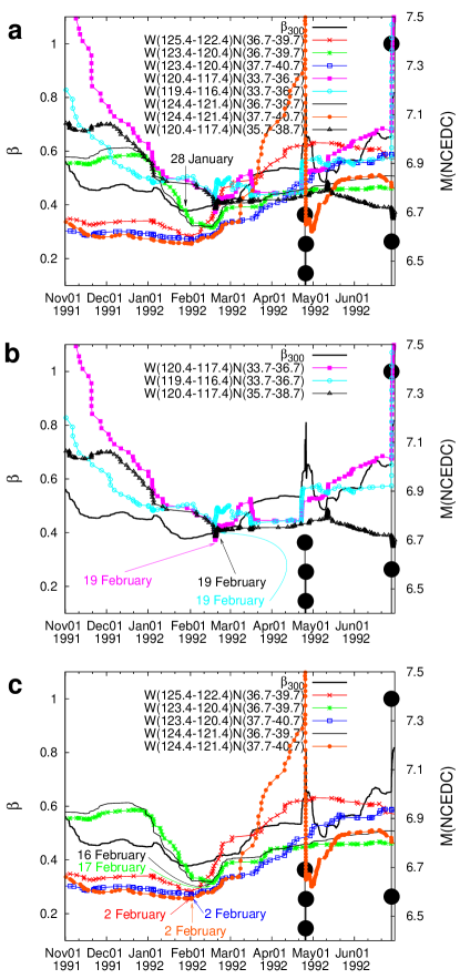
Figure 3: (color online) Results for the $M$7.4 Landers EQ in California on 28 June 1992, and for the Cape Mendocino EQ on 25 April 1992. (a) The variability $\beta$ of the seismicity versus the conventional time for a natural time window length $W$ comprising a number of events that would occur in three months: The black thick curve resulting from the wide area $N_{31.7}^{45.7}W_{127.5}^{112.1}$ exhibits a very broad minimum approximately from 18 January to 20 February 1992 with its lowest value on 28 January 1992, as marked. The other eight curves correspond to those areas -among the 38 encircled ones in Fig. 1- leading to $\beta$ minima at dates within the range of the broad minimum of the wide area. These dates are marked in (b) for the three curves that correspond to areas related with the Landers EQ and in (c) for the remaining five curves corresponding to areas associated with the Cape Mendocino EQ (see the text). The cyan curve in (b) corresponds to the area $N_{33.7}^{36.7}W_{119.4}^{116.4}$ depicted in Fig. 1 with the cyan rectangle that includes the Landers EQ epicenter (the largest red triangle). The curve with the orange circles in (c) corresponds to the area $N_{37.7}^{40.7}W_{124.4}^{121.4}$, shown in Fig. 1 with the orange rectangle surrounding the Cape Mendocino EQ epicenter. The EQs with $M\geq 6.4$ (right scale) are shown with vertical bars ending at solid circles.

VI Discussion and Conclusions

The prediction of the epicenter of an impending mainshock can be made on the basis of the SES physical properties, as mentioned in the Introduction. This of course has two prerequisites: First, that geoelectrical data are available and second, that we know from earlier experience the selectivity map Varotsos et al. (1996) of the measuring station at which the SES under investigation appeared. The method proposed here cannot be falsely considered as replacing that followed by means of SES since it does not improve its accuracy, which is of the order of 100km, but it has the privilege that can be applied even in the lack of geoelectrical data.

In conclusion, here we proposed a method to estimate the epicentral area of an impending mainshock based on a precursory minimum observed in the fluctuations of the order parameter of seismicity. This has been successfully applied to mainshocks in California including the Landers EQ on 28 June 1992, which is the largest earthquake that occurred in California during the last three decades. These results are found to be robust when repeating 100 trials upon considering a reasonable experimental error in the magnitude measurements of the earthquakes in the seismic catalog used.

VII Methods

All the seismic data taken from NCEDC have been analyzed in natural time. The seismic moment $M_{0}$, which is proportional to the energy release during an earthquake and hence to the quantity $Q_{k}$ used in natural time analysis, is calculated Varotsos et al. (2011b) from the relation $\log_{10}(M_{0})=1.5M+$const.

References

- Turcotte (1997) D. L. Turcotte, Fractals and Chaos in Geology and Geophysics (Cambridge University Press, Cambridge, 1997), 2nd ed.
- Holliday et al. (2006) J. R. Holliday, J. B. Rundle, D. L. Turcotte, W. Klein, K. F. Tiampo, and A. Donnellan, Phys. Rev. Lett. 97, 238501 (2006).
- Huang (2008) Q. Huang, Geophys. Res. Lett. 35, L23308 (2008).
- Telesca (2010) L. Telesca, Tectonophysics 494, 155 (2010).
- Lennartz et al. (2011) S. Lennartz, A. Bunde, and D. L. Turcotte, Geophys. J. Int. 184, 1214 (2011).
- Lippiello et al. (2012) E. Lippiello, C. Godano, and L. de Arcangelis, Geophys. Res. Lett. 39, L05309 (2012).
- Tenenbaum et al. (2012) J. N. Tenenbaum, S. Havlin, and H. E. Stanley, Phys. Rev. E 86, 046107 (2012).
- Varotsos et al. (2002a) P. A. Varotsos, N. V. Sarlis, and E. S. Skordas, Phys. Rev. E 66, 011902 (2002a).
- Varotsos et al. (2002b) P. A. Varotsos, N. V. Sarlis, and E. S. Skordas, Acta Geophysica Polonica 50, 337 (2002b).
- Tanaka et al. (2004) H. K. Tanaka, P. A. Varotsos, N. V. Sarlis, and E. S. Skordas, Proc. Jpn. Acad. Ser. B Phys. Biol. Sci. 80, 283 (2004).
- Varotsos et al. (2011a) P. Varotsos, N. V. Sarlis, E. S. Skordas, S. Uyeda, and M. Kamogawa, Proc. Natl. Acad. Sci. USA 108, 11361 (2011a).
- Varotsos et al. (2011b) P. A. Varotsos, N. V. Sarlis, and E. S. Skordas, Natural Time Analysis: The new view of time. Precursory Seismic Electric Signals, Earthquakes and other Complex Time-Series (Springer-Verlag, Berlin Heidelberg, 2011b).
- Varotsos and Alexopoulos (1984) P. Varotsos and K. Alexopoulos, Tectonophysics 110, 73 (1984).
- Varotsos et al. (2013) P. A. Varotsos, N. V. Sarlis, E. S. Skordas, and M. S. Lazaridou, Tectonophysics 589, 116 (2013).
- Varotsos and Alexopoulos (1978) P. Varotsos and K. Alexopoulos, Phys. Status Solidi A 47, K133 (1978).
- Varotsos (1980) P. Varotsos, physica status solidi (b) 100, K133 (1980).
- Varotsos et al. (1982) P. Varotsos, K. Alexopoulos, and K. Nomicos, physica status solidi (b) 111, 581 (1982).
- Varotsos and Alexopoulos (1982) P. Varotsos and K. Alexopoulos, physica status solidi (b) 110, 9 (1982).
- Varotsos (2008) P. Varotsos, Solid State Ionics 179, 438 (2008).
- Varotsos et al. (1996) P. Varotsos, K. Eftaxias, M. Lazaridou, K. Nomicos, N. Sarlis, N. Bogris, J. Makris, G. Antonopoulos, and J. Kopanas, Acta Geophysica Polonica 44, 301 (1996).
- Varotsos et al. (2003a) P. A. Varotsos, N. V. Sarlis, and E. S. Skordas, Phys. Rev. E 67, 021109 (2003a).
- Varotsos et al. (2003b) P. A. Varotsos, N. V. Sarlis, and E. S. Skordas, Phys. Rev. E 68, 031106 (2003b).
- Varotsos et al. (2006) P. A. Varotsos, N. V. Sarlis, E. S. Skordas, H. K. Tanaka, and M. S. Lazaridou, Phys. Rev. E 74, 021123 (2006).
- Sarlis et al. (2008) N. V. Sarlis, E. S. Skordas, M. S. Lazaridou, and P. A. Varotsos, Proc. Jpn. Acad. Ser. B Phys. Biol. Sci. 84, 331 (2008).
- Sarlis et al. (2013) N. V. Sarlis, E. S. Skordas, P. A. Varotsos, T. Nagao, M. Kamogawa, H. Tanaka, and S. Uyeda, Proc. Natl. Acad. Sci. USA 110, 13734 (2013).
- Sarlis et al. (2015) N. V. Sarlis, E. S. Skordas, P. A. Varotsos, T. Nagao, M. Kamogawa, and S. Uyeda, Proc. Natl. Acad. Sci. USA 112, 986 (2015).
- Varotsos et al. (2005) P. A. Varotsos, N. V. Sarlis, H. K. Tanaka, and E. S. Skordas, Phys. Rev. E 72, 041103 (2005).
- Kanamori (1978) H. Kanamori, Nature 271, 411 (1978).
- Sarlis et al. (2010) N. V. Sarlis, E. S. Skordas, and P. A. Varotsos, EPL 91, 59001 (2010).
- Bramwell et al. (1998) S. T. Bramwell, P. C. W. Holdsworth, and J. F. Pinton, Nature (London) 396, 552 (1998).
- Bramwell et al. (2001) S. T. Bramwell, J.-Y. Fortin, P. C. W. Holdsworth, S. Peysson, J.-F. Pinton, B. Portelli, and M. Sellitto, Phys. Rev. E 63, 041106 (2001).
- Zheng and Trimper (2001) B. Zheng and S. Trimper, Phys. Rev. Lett. 87, 188901 (2001).
- Zheng (2003) B. Zheng, Phys. Rev. E 67, 026114 (2003).
- Clusel et al. (2004) M. Clusel, J.-Y. Fortin, and P. C. W. Holdsworth, Phys. Rev. E 70, 046112 (2004).
- Aegerter et al. (2004) C. M. Aegerter, M. S. Welling, and R. J. Wijngaarden, Europhys. Lett. 65, 753 (2004).
- Lőrincz and Wijngaarden (2007) K. A. Lőrincz and R. J. Wijngaarden, Phys. Rev. E 76, 040301 (2007).
- Sarlis et al. (2011) N. Sarlis, E. Skordas, and P. Varotsos, EPL 96, 28006 (2011).
- Bak et al. (1987) P. Bak, C. Tang, and K. Wiesenfeld, Phys. Rev. Lett. 59, 381 (1987).
- Varotsos et al. (2012) P. Varotsos, N. Sarlis, and E. Skordas, EPL 99, 59001 (2012).
- Uyeda et al. (2002) S. Uyeda, M. Hayakawa, T. Nagao, O. Molchanov, K. Hattori, Y. Orihara, K. Gotoh, Y. Akinaga, and H. Tanaka, Proc. Natl. Acad. Sci. USA 99, 7352 (2002).
- Peng et al. (1994) C.-K. Peng, S. V. Buldyrev, S. Havlin, M. Simons, H. E. Stanley, and A. L. Goldberger, Phys. Rev. E 49, 1685 (1994).
- Varotsos et al. (2014) P. A. Varotsos, N. V. Sarlis, and E. S. Skordas, J. Geophys. Res.: Space Physics 119, 9192 (2014).
- Hu et al. (2001) K. Hu, P. C. Ivanov, Z. Chen, P. Carpena, and H. E. Stanley, Phys. Rev. E 64, 011114 (2001).
- Chen et al. (2002) Z. Chen, P. C. Ivanov, K. Hu, and H. E. Stanley, Phys. Rev. E 65, 041107 (2002).
- Chen et al. (2005) Z. Chen, K. Hu, P. Carpena, P. Bernaola-Galvan, H. E. Stanley, and P. C. Ivanov, Phys. Rev. E 71, 011104 (2005).
- Ma et al. (2010) Q. D. Y. Ma, R. P. Bartsch, P. Bernaola-Galván, M. Yoneyama, and P. C. Ivanov, Phys. Rev. E 81, 031101 (2010).
- Xu et al. (2011) Y. Xu, Q. D. Ma, D. T. Schmitt, P. Bernaola-Galván, and P. C. Ivanov, Physica A 390, 4057 (2011).
- Tanioka et al. (1995) Y. Tanioka, K. Satake, and L. Ruff, Tectonics 14, 1095 (1995).