Sequential Detection of Three-Dimensional Signals under Dependent Noise

Abstract

Abstract: We study detection methods for multivariable signals under dependent noise. The main focus is on three-dimensional signals, i.e. on signals in the space-time domain. Examples for such signals are multifaceted. They include geographic and climatic data as well as image data, that are observed over a fixed time horizon. We assume that the signal is observed as a finite block of noisy samples whereby we are interested in detecting changes from a given reference signal. Our detector statistic is based on a sequential partial sum process, related to classical signal decomposition and reconstruction approaches applied to the sampled signal. We show that this detector process converges weakly under the no change null hypothesis that the signal coincides with the reference signal, provided that the spatial-temporal partial sum process associated to the random field of the noise terms disturbing the sampled signal converges to a Brownian motion. More generally, we also establish the limiting distribution under a wide class of local alternatives that allows for smooth as well as discontinuous changes. Our results also cover extensions to the case that the reference signal is unknown. We conclude with an extensive simulation study of the detection algorithm.
 
Keywords: Change-point problems; Correlated noise random fields; Image processing; Multivariate Brownian motion; Sampling theorems; Sequential detection.

1 Introduction

Signal processing and signal transmission play an important role in many different areas. Typical problems include the reconstruction of a signal by its discretely sampled values as well as the detection of changes from a given reference signal. For univariate signals $f\colon\mathbb{R}\to\mathbb{R}$, sampled equidistantly using a sampling period $\tau>0$ and disturbed by additive noise, such that one obtains a block of noisy samples $\{y_{\bm{i}}:i\in\{1,\ldots,n\}\}$ where

$$y_{\bm{i}}=f\left(i\tau\right)+\varepsilon_{\bm{i}},$$ (1.1)

a nonparametric joint reconstruction/detection algorithm has been proposed in the paper of Pawlak and Steland (2013). Their approach has several appealing features. Firstly, the algorithm can detect changes while reconstructing the signal at the same time. Secondly, it is a nonparametric approach, i.e. no further information about the exact class to which the observed signal belongs is necessary. Lastly, the procedure works in a sequential way such that changes can be detected on-line, in contrast to off-line detection schemes which can first detect changes in retrospect, i.e. when the whole data set is already available.

A natural question arises whether this approach also works for high-dimensional signals. One answer to this problem is given in Prause and Steland (2015), where the authors treat matrix-valued signals and apply results from Pawlak and Steland (2013) by considering quadratic forms. In the present paper, however, we consider a more general framework by focusing our attention on signals $f\colon\mathbb{R}^{q}\to\mathbb{R}$ for $q>1$. Examples for such signals are multifaceted, including geographic and climatic data as well as image data, that are observed over a fixed time horizon. In order to simplify the notation we fix $q=3$ as this case also covers the most interesting applications. However, our results also hold true for $q=2$ and arbitrary $q>3$ and the corresponding proofs can easily be completed along the same lines. Thus, in the following we are interested in reconstructing three-dimensional signals and, at the same time, in detecting changes from a given reference signal. Here, one component represents the time and the other two the location. The application that we have in mind are video signals, i.e. sequences of image frames over time.

The basis on which we now want to establish our investigations is a finite block of noisy samples $\{y_{\bm{i}}=y_{i_{1},i_{2},i_{3}}:(i_{1},i_{2},i_{3})\in\{1,\ldots,n_{1}\}\times\{1,\ldots,n_{2}\}\times\{1,\ldots,n_{3}\}\}$ that – in accordance with model (1.1) – is obtained from the model

$$y_{i_{1},i_{2},i_{3}}=f\left(i_{1}\tau_{1},i_{2}\tau_{2},i_{3}\tau_{3}\right)+\varepsilon_{i_{1},i_{2},i_{3}}\,.$$ (1.2)

Here, $f(t,r_{2},r_{3})$ is the unknown signal depending on time ($i_{1}$) and location ($i_{2}$ and $i_{3}$), $\left\{\varepsilon_{\bm{i}}=\varepsilon_{i_{1},i_{2},i_{3}}\right\}$ is a zero mean random field and $\tau_{j}=\tau_{n_{j}},\,j=1,2,3$, are the sampling periods. We assume that they fulfill $\tau_{j}\to 0$ and $n_{j}\tau_{j}\to\overline{\tau}_{j}$, $j=1,2,3$ as $\min_{1\leq i\leq 3}n_{i}\to\infty$. As in Pawlak and Steland (2013) we want to base our approaches on classical reconstruction procedures from the signal sampling theory, leading to sequential partial sum processes as detector statistics, see Section 2. In order to make these detector statistics applicable we need to determine proper control limits; thus, in Section 3 we will show that we can generalize the two main weak convergence results in Pawlak and Steland (2013) to our multidimensional context, i.e. we show weak convergence of the detection process towards Gaussian processes under different assumptions on the dependence structure of the noise processes where either the null hypothesis $f=f_{0}$ or the alternative $f\neq f_{0}$ holds true. In Section 4 we present extensions to weighting functions, which allow to detect the location of the change as well, and discuss how to treat the case of an unknown but time-constant reference signal. Finally, in Section 5 we present some simulation results concerning the rejection rates and the power of the detection algorithm.

2 The detection algorithm

We now want to extend the main results of Pawlak and Steland (2013) to signals $f\colon\mathbb{R}^{q}\to\mathbb{R}$ with $q=3$. As in Pawlak and Steland (2013) we base our estimator of $f(t,r_{2},r_{3})$ on results of the signal sampling theory like the Shannon-Whittaker theorem. This theorem has generalizations to signals with several variables. In three dimensions we have for band-limited functions on $[-\Omega_{1},\Omega_{1}]\times[-\Omega_{2},\Omega_{2}]\times[-\Omega_{3},\Omega_{3}]$ with $0<\Omega_{1},\Omega_{2},\Omega_{3}<\infty$ the representation

$$f(t,r_{2},r_{3})= \sum_{i_{1}=-\infty}^{\infty}\sum_{i_{2}=-\infty}^{\infty}\sum_{i_{3}=-\infty}^{\infty}f\left(\frac{i_{1}\pi}{\Omega_{1}},\frac{i_{2}\pi}{\Omega_{2}},\frac{i_{3}\pi}{\Omega_{3}}\right)$$

$$\ \ \textnormal{sinc}\left(\Omega_{1}\left(t-\frac{i_{1}\pi}{\Omega_{1}}\right)\right)\textnormal{sinc}\left(\Omega_{2}\left(r_{2}-\frac{i_{2}\pi}{\Omega_{2}}\right)\right)\textnormal{sinc}\left(\Omega_{3}\left(r_{3}-\frac{i_{3}\pi}{\Omega_{3}}\right)\right),$$

where $\textnormal{sinc}(x)=\frac{\sin(x)}{x}$, cf. Jerri (1977), p. 1571. The most direct idea to construct an estimator of $f(t,r_{2},r_{3})$ would now be to just replace the values of $f$ at $\left(i_{1}\pi/\Omega_{1},i_{2}\pi/\Omega_{2},i_{3}\pi/\Omega_{3}\right)$ by the noisy observations $y_{\bm{i}}=y_{i_{1},i_{2},i_{3}}$. However, Pawlak and Stadtmüller (1996) have shown that this naive estimator is not even consistent in one dimension. Instead, they propose a post-filtering correction of the so-called oversampled version of the Shannon-Whittaker series to filter out high frequencies. This is the approach that we also adapt here. In three dimensions this oversampled version is of the form

$$f(t,r_{2},r_{3})= \sum_{i_{1}=-\infty}^{\infty}\sum_{i_{2}=-\infty}^{\infty}\sum_{i_{3}=-\infty}^{\infty}f\left(i_{1}\tau_{1},i_{2}\tau_{2},i_{3}\tau_{3}\right)$$

$$\ \ \textnormal{sinc}(\pi\tau_{1}^{-1}(t-i_{1}\tau_{1}))\textnormal{sinc}(\pi\tau_{2}^{-1}(r_{2}-i_{2}\tau_{2}))\textnormal{sinc}(\pi\tau_{3}^{-1}(r_{3}-i_{3}\tau_{3}))$$

for $0<\tau_{j}\leq\pi/\Omega_{j},j=1,2,3$. If we convolve this version with

$$g(t,r_{2},r_{3})=\frac{\Omega_{1}\Omega_{2}\Omega_{3}}{\pi^{3}}\textnormal{sinc}(\Omega_{1}t)\textnormal{sinc}(\Omega_{2}r_{2})\textnormal{sinc}(\Omega_{3}r_{3}),$$

use the fact that

$$\quad\ \textnormal{sinc}(\pi\tau_{1}^{-1}(t-i_{1}\tau_{1}))\textnormal{sinc}(\pi\tau_{2}^{-1}(r_{2}-i_{2}\tau_{2}))\textnormal{sinc}(\pi\tau_{3}^{-1}(r_{3}-i_{3}\tau_{3}))\ast g(t,r_{2},r_{3})$$

$$=\tau_{1}\tau_{2}\tau_{3}\frac{\Omega_{1}\Omega_{2}\Omega_{3}}{\pi^{3}}\textnormal{sinc}(\Omega_{1}(t-i_{1}\tau_{1}))\textnormal{sinc}(\Omega_{2}(r_{2}-i_{1}\tau_{2}))\textnormal{sinc}(\Omega_{3}(r_{3}-i_{1}\tau_{3})),$$

and replace $f\left(i_{1}\tau_{1},i_{2}\tau_{2},i_{3}\tau_{3}\right)$ by the noisy sample $y_{i_{1},i_{2},i_{3}}$, this finally leads to the following truncated convolution form as an estimator for $f(t,r_{2},r_{3}),$ namely

$$\widehat{f}_{n_{1},n_{2},n_{3}}(t,r_{2},r_{3})\coloneqq\tau_{1}\tau_{2}\tau_{3}\sum_{i_{1}=1}^{n_{1}}\sum_{i_{2}=1}^{n_{2}}\sum_{i_{3}=1}^{n_{3}}y_{i_{1},i_{2},i_{3}}\varphi\left(t-i_{1}\tau_{1},r_{2}-i_{2}\tau_{2},r_{3}-i_{3}\tau_{3}\right),$$

cf. Pawlak and Stadtmüller (1996), p. 1427, and Pawlak and Stadtmüller (2007), p. 2527. Here,

$$\varphi(t,r_{2},r_{3})=\frac{\sin(\Omega_{1}t)}{\pi t}\frac{\sin(\Omega_{2}r_{2})}{\pi r_{2}}\frac{\sin(\Omega_{3}r_{3})}{\pi r_{3}}\eqqcolon\widetilde{\varphi}_{1}(t)\widetilde{\varphi}_{2}(r_{2})\widetilde{\varphi}_{3}(r_{3})$$

is a three-dimensional product reconstruction kernel with $\widetilde{\varphi}_{j}(0)=\Omega_{j}/\pi$ for $j=1,2,3$.

Given a reference signal $f_{0}(t,r_{2},r_{3})$, our aim now is to decide whether or not we can reject the null hypothesis

$$H_{0}:f(t,r_{2},r_{3})=f_{0}(t,r_{2},r_{3})$$

for all $t\in[0,\overline{\tau}_{1}],r_{2}\in[0,\overline{\tau}_{2}],r_{3}\in[0,\overline{\tau}_{3}]$. As we receive our data in a sequential way over time as a sequence of image frames, we want to be able to detect changes as early as possible, i.e. we want to give an alarm as soon as we have enough evidence in our samples

$$\left\{y_{i_{1},i_{2},i_{3}}:i_{1}\in\{1,\ldots,k\},i_{2}\in\{1,\ldots,n_{2}\},i_{3}\in\{1,\ldots,n_{3}\}\right\},$$

corresponding to the first $k$ image frames, to reject the null hypothesis. To achieve this aim we consider a sequential partial sum process over time which is defined as

$$\mathcal{F}_{n}(s,t,r_{2},r_{3}) \coloneqq(\tau_{1}\tau_{2}\tau_{3})^{-1/2}(\widehat{f}_{\left\lfloor n_{1}s\right\rfloor}(t,r_{2},r_{3})-\mathbb{E}_{0}\widehat{f}_{\left\lfloor n_{1}s\right\rfloor}(t,r_{2},r_{3}))$$

$$=\sqrt{\tau_{1}\tau_{2}\tau_{3}}\sum_{l_{1}=1}^{\lfloor n_{1}s\rfloor}\sum_{l_{2}=1}^{n_{2}}\sum_{l_{3}=1}^{n_{3}}\left[y_{l_{1},l_{2},l_{3}}-f_{0}(l_{1}\tau_{1},l_{2}\tau_{2},l_{3}\tau_{3})\right]$$

$$\hskip 122.34692pt\varphi\left(t-l_{1}\tau_{1},r_{2}-l_{2}\tau_{2},r_{3}-l_{3}\tau_{3}\right),$$ (2.1)

for $0<s_{0}\leq s\leq 1,t\in[0,\overline{\tau}_{1}],r_{2}\in[0,\overline{\tau}_{2}],r_{3}\in[0,\overline{\tau}_{3}]$. The subscript $n$ denotes the dependence on the sample sizes. Note that $\mathbb{E}_{0}$ denotes as usual the expectation taken under the null hypothesis. With this process we can easily define detectors such as the local detector

$$\mathcal{L}_{n}\coloneqq\min\left\{n_{0}\leq k\leq n_{1}:\max_{r_{2}\in[0,\overline{\tau}_{2}],\atop r_{3}\in[0,\overline{\tau}_{3}]}\left|\mathcal{F}_{n}\left(\frac{k}{n_{1}},\frac{\overline{\tau}_{1}k}{n_{1}},r_{2},r_{3}\right)\right|>c_{L}\right\}$$ (2.2)

or the global maximum norm detector

$$\mathcal{M}_{n}\coloneqq\min\left\{n_{0}\leq k\leq n_{1}:\max_{0\leq t\leq\overline{\tau}_{1}k/n_{1}}\max_{r_{2}\in[0,\overline{\tau}_{2}],\atop r_{3}\in[0,\overline{\tau}_{3}]}\left|\mathcal{F}_{n}\left(\frac{k}{n_{1}},t,r_{2},r_{3}\right)\right|>c_{M}\right\}$$ (2.3)

with control limits $c_{L}>0$ and $c_{M}>0$ and $n_{0}\coloneqq\lfloor n_{1}s_{0}\rfloor$, $s_{0}\in(0,1)$. The reason to start monitoring in $n_{0}$ is that we assume that we have a kind of learning sample, i.e. we assume

$$f(t,r_{2},r_{3})=f_{0}(t,r_{2},r_{3}),\ 0\leq t\leq s_{0}\overline{\tau}_{1},0<s_{0}<1.$$ (2.4)

This assumption guarantees that no initial change in the signal occurs before the monitoring procedure starts which allows to estimate unknown parameters of the detection process such as the asymptotic variance $\sigma^{2}$, see below.

Now the question arises how to reasonably choose the control parameters $c_{L}$ and $c_{M}$. To answer this question we are interested in the limiting distribution of our detector statistics. These can be derived from the limiting distribution of our stochastic process $\mathcal{F}_{n}(s,t,r_{2},r_{3})$ which is subject of the next section.

3 Process limit distributions

The asymptotic results to be discussed now, under the null hypothesis of no change and a rich class of alternative hypotheses under which the true signal converges to the reference signal, are based on a weak assumption about the asymptotic distribution of the partial sum process of the random field $\left\{\varepsilon_{i_{1},i_{2},i_{3}}\right\}$. Before discussing that assumption and providing the asymptotic results, we introduce some preliminaries and notations used in the sequel.

3.1 Preliminaries

As usual, the cardinality of a set $u\subseteq\{1,\ldots,q\}$ is denoted as $|u|$. Moreover, for $v\subseteq\{1,\ldots,q\}$ we write $u-v$ for the complement of $v$ with respect to $u$. In particular, we just write $-v$ if we take the complement of $v$ with respect to the whole set $\{1,\ldots,q\}$. Sets of the form $\{j,j+1,\ldots,k\}$ for integers $j$ and $k$ with $j\leq k$ are abbreviated as $j:k$, such that $\{1,\ldots,q\}=1:q$.

To pick out the components of a vector $\bm{x}\in\mathbb{R}^{q}$ that correspond to a set $u\subseteq 1:q$, we write $\bm{x}_{u}$, i.e. $\bm{x}_{u}$ stands for a vector with $|u|$ components with selected entries of $\bm{x}$. Now, let $u,v\subseteq 1:q$ and $\bm{x},\bm{z}\in[\bm{a},\bm{b}]$ with $u\cap v=\emptyset$. The symbol $\bm{x}_{u}:\bm{z}_{v}$ then denotes the point $\bm{y}\in\left[\bm{a}_{u\cup v},\bm{b}_{u\cup v}\right]$, where $y_{j}=x_{j}$ for all $j\in u$ and $y_{j}=z_{j}$ for all $j\in v$.

Recall the concept of the $q$-fold alternating sum of a function $f$ over the hyperrectangle $[\bm{a},\bm{b}]$ which is defined as

$$\Delta(f;\bm{a},\bm{b})\coloneqq\sum_{v\subseteq\{1,\ldots,q\}}(-1)^{|v|}f\left(\bm{a}_{v}:\bm{b}_{-v}\right).$$ (3.1)

Now, let $W$ be a subset of $[0,1]^{q}$. For points in $[0,1]^{q}$ set $\bm{t}=(t_{1},\ldots,t_{q})$ and $\bm{s}=(s_{1},\ldots,s_{q})$ respectively. We call $W$ a block if it is of the form

$$W\coloneqq\prod_{j=1}^{q}(s_{j},t_{j}],$$

where each $(s_{j},t_{j}],j=1,\ldots,q$ is a left-open, right-closed subintervals of $[0,1]$. We now define the increment $X(W)$ of a stochastic process $X=\{X(\bm{t}):\bm{t}\in[0,1]^{q}\}$ around a block $W$ by means of the alternating sum (3.1) as

$$X(W)\coloneqq\Delta(X;\bm{s},\bm{t})=\sum_{v\subseteq\{1,\ldots,q\}}(-1)^{|v|}X\left(\bm{s}_{v}:\bm{t}_{-v}\right).$$

We are now able to define the Brownian motion on $[0,1]^{q}$, cf. Deo (1975), p. 709, where $C_{q}$ stands for the space of all real-valued continuous functions on $[0,1]^{q}$.

Definition 3.1.

The Brownian motion $B=\{B(\bm{t}):\bm{t}\in[0,1]^{q}\}$ on $[0,1]^{q}$ is characterized by

• $P(B\in C_{q})=1$,

• if $W_{1},\ldots,W_{k}$ are pairwise disjoint blocks in $[0,1]^{q}$, then the increments

  $$B(W_{1}),\ldots,B(W_{k})$$

  are independent normal random variables with means zero and variances

  $$\lambda(W_{1}),\ldots,\lambda(W_{k}),$$

  $\lambda$ being the $q$-dimensional Lebesgue measure on $[0,1]^{q}$.

We can now formulate the main assumption for the asymptotic theory of the detection process as follows, where $\Rightarrow$ – as usual – stands for weak convergence in an appropriately chosen function space, see Appendix A.1.

Assumption 1: Let $\{\varepsilon_{i_{1},i_{2},i_{3}}\}$ be a weakly stationary random field with $\mathbb{E}(\varepsilon_{\bm{i}})=0$ which satisfies a functional central limit theorem, i.e.

$$Z_{n}(v_{1},v_{2},v_{3})\coloneqq(n_{1}n_{2}n_{3})^{-1/2}\sum_{i_{1}=1}^{\lfloor n_{1}v_{1}\rfloor}\sum_{i_{2}=1}^{\lfloor n_{2}v_{2}\rfloor}\sum_{i_{3}=1}^{\lfloor n_{3}v_{3}\rfloor}\varepsilon_{i_{1},i_{2},i_{3}}\Rightarrow\sigma B (v_{1},v_{2},v_{3}),$$ (3.2)

$$(v_{1},v_{2},v_{3})\in[0,1]^{3},$$

in the Skorohod space $D[0,1]^{3}$ as $\min_{1\leq i\leq 3}n_{i}\to\infty$ for some constant $\sigma^{2}\in(0,\infty)$.

Here, the constant $\sigma^{2}$ equals the long-run variance of the random field $\{\varepsilon_{i_{1},i_{2},i_{3}}\}$, i.e.

$$\sigma^{2}\coloneqq\lim_{\min_{1\leq i\leq 3}n_{i}\to\infty}\mathbb{V}\textnormal{ar}\left((n_{1}n_{2}n_{3})^{-1/2}\sum_{i_{1}=1}^{n_{1}}\sum_{i_{2}=1}^{n_{2}}\sum_{i_{3}=1}^{n_{3}}\varepsilon_{i_{1},i_{2},i_{3}}\right)=\sum_{\bm{k}\in\mathbb{Z}^{3}}\mathbb{E}(\varepsilon_{\bm{0}}\varepsilon_{\bm{k}}).$$

There exist several results in the literature about the weak invariance principle (3.2) under specific conditions on the random field. In particular, in the i.i.d. case we get the functional central limit theorem under the sole assumptions that

$$\mathbb{E}(\xi_{\bm{0}})=0,\ \mathbb{E}\left(\xi_{\bm{0}}^{2}\right)<\infty\ \textnormal{and}\ \sigma^{2}>0,$$

see Corollary 1 in Wichura (1969). More generally, a functional central limit theorem for strictly stationary and $\varphi$-mixing random fields can be found in Deo (1975), cf. Theorem 1. Further results on weak invariance principles for random fields include weakly stationary associated as well as weakly stationary and $\alpha$-mixing random fields, cf. Bulinski and Kaene (1996), p. 2906, and Berkes and Morrow (1981), Theorem 1, respectively. The latter obtain a strong approximation of the partial sum field by a Brownian motion from which one can deduce a weak invariance principle quite directly. Other results on functional central limit theorems for random fields include the ones of Wang and Woodroofe (2013), cf. Theorem 1.1, and Machkouri et al. (2013), cf. Theorem 2. These authors consider random fields of the form $X_{\bm{i}}=g(\varepsilon_{\bm{i}-\bm{s}};\bm{s}\in\mathbb{Z}^{q})$ where $g$ is a measurable function and the $\{\varepsilon_{\bm{j}};\bm{j}\in\mathbb{Z}^{q}\}$ are i.i.d. random variables. Machkouri et al. (2013) introduce the notion of a $p$-stable random field and then obtain a weak invariance principle for the so-called smoothed partial sum process.

3.2 Asymptotics under the Null Hypothesis

With the help of Assumption 1 we are now in a position to formulate the following theorem stating the asymptotic behaviour of the process.

Theorem 3.1.

Suppose the noise process $\{\varepsilon_{\bm{i}}=\varepsilon_{i_{1},i_{2},i_{3}}\}$ meets Assumption 1. Assume that the sampling periods fulfill $n_{j}\tau_{j}\to\overline{\tau}_{j}$ for $j=1,2,3,$ as $\min_{1\leq i\leq 3}n_{i}\to\infty$. Then, under the null hypothesis $H_{0}$, we have

$$\mathcal{F}_{n}(s,t,r_{2},r_{3})\Rightarrow\mathcal{F}(s,t,r_{2},r_{3}),$$

as $\min_{1\leq i\leq 3}n_{i}\to\infty$ for $0<s_{0}\leq s\leq 1$, $t\in[0,\overline{\tau}_{1}]$, $r_{2}\in[0,\overline{\tau}_{2}]$ and $r_{3}\in[0,\overline{\tau}_{3}]$.

The limit stochastic process $\mathcal{F}(s,t,r_{2},r_{3})$ is of the form

$$\mathcal{F}(s,t,r_{2},r_{3})\coloneqq\sqrt{\overline{\tau}_{1}\overline{\tau}_{2}\overline{\tau}_{3}}\,\sigma\int_{0}^{s}\int_{0}^{1}\int_{0}^{1} \!\varphi\left(t-\overline{\tau}_{1}z_{1},r_{2}-\overline{\tau}_{2}z_{2},r_{3}-\overline{\tau}_{3}z_{3}\right)$$

$$\mathrm{d}B(z_{1},z_{2},z_{3}),$$

where $B(z_{1},z_{2},z_{3})$ is the standard Brownian motion on $[0,1]^{3}$.

The weak convergence takes place in a higher dimensional Skorohod space and the last integral is interpreted as multivariate Riemann-Stieltjes integral, see Appendix A.1 for more details.

The next lemma is a characterization of the correlation structure of the limit process $\mathcal{F}(s,t,r_{2},r_{3})$.

Lemma 3.1.

• The process $\mathcal{F}(s,t,r_{2},r_{3})$ is a nonstationary multivariable Gaussian process with

  $$\mathbb{E}(\mathcal{F}(s,t,r_{2},r_{3}))=\bm{0}$$

  and covariance function

  $$\quad\ \mathbb{C}\textnormal{ov}\left(\mathcal{F}(s^{(1)},t^{(1)},r^{(1)}_{2},r^{(1)}_{3}),\mathcal{F}(s^{(2)},t^{(2)},r^{(2)}_{2},r^{(2)}_{3})\right)$$

  $$=\sigma^{2}\overline{\tau}_{1}\overline{\tau}_{2}\overline{\tau}_{3}\int_{0}^{\min\{s^{(1)},s^{(2)}\}}\int_{0}^{1}\int_{0}^{1}\!\varphi(t^{(1)}-\overline{\tau}_{1}z_{1},r^{(1)}_{2}-\overline{\tau}_{2}z_{2},r^{(1)}_{3}-\overline{\tau}_{3}z_{3})$$

  $$\hskip 85.35826pt\varphi(t^{(2)}-\overline{\tau}_{1}z_{1},r^{(2)}_{2}-\overline{\tau}_{2}z_{2},r^{(2)}_{3}-\overline{\tau}_{3}z_{3})\,\mathrm{d}z_{3}\mathrm{d}z_{2}\mathrm{d}z_{1}$$ (3.3)

  for $0<s_{0}\leq s^{(1)},s^{(2)}\leq 1$, $0\leq t^{(1)},t^{(2)}\leq\overline{\tau}_{1}$, $0\leq r^{(1)}_{2},r^{(2)}_{2}\leq\overline{\tau}_{2}$, and $0\leq r^{(1)}_{3},r^{(2)}_{3}\leq\overline{\tau}_{3}$.

• The process $\mathcal{F}(s,t,r_{2},r_{3})$ has continuous sample paths.

Now that we have the limit distribution of $\mathcal{F}_{n}(s,t,r_{2},r_{3})$ under the null hypothesis at our disposal, we can easily derive central limit theorems for the local and global maximum norm detector defined in (2.2) and (2.3).

Lemma 3.2.

Assume that condition (2.4) holds true. Then, under the conditions of Theorem 3.1 the detectors satisfy the following central limit theorems:

$$\mathcal{L}_{n}/n_{1}\Rightarrow\mathcal{L}\coloneqq\inf\left\{s\in[s_{0},1]:\sup_{r_{2}\in[0,\overline{\tau}_{2}],\atop r_{3}\in[0,\overline{\tau}_{3}]}\left|\mathcal{F}(s,s\overline{\tau}_{1},r_{2},r_{3})\right|>c_{L}\right\},$$

$$\mathcal{M}_{n}/n_{1}\Rightarrow\mathcal{M}\coloneqq\inf\left\{s\in[s_{0},1]:\sup_{0\leq t\leq s\overline{\tau}_{1}}\sup_{r_{2}\in[0,\overline{\tau}_{2}],\atop r_{3}\in[0,\overline{\tau}_{3}]}\left|\mathcal{F}(s,t,r_{2},r_{3})\right|>c_{M}\right\},$$

as $\min_{1\leq i\leq 3}n_{i}\to\infty$.

3.3 Asymptotics under the Alternative

We now investigate the behaviour of our statistic $\mathcal{F}_{n}(s,t,r_{2},r_{3})$ under a general class of alternatives $H_{1}:f_{n_{1},n_{2},n_{3}}(t,r_{2},r_{3})\neq f_{0}(t,r_{2},r_{3})$, i.e. in the situation when the observed signal and the reference signal differ. We assume that our observed data $\{y_{\bm{i}}=y_{i_{1},i_{2},i_{3}}:(i_{1},i_{2},i_{3})\in\{1,\ldots,n_{1}\}\times\{1,\ldots,n_{2}\}\times\{1,\ldots,n_{3}\}\}$ obey the following model:

$$y_{i_{1},i_{2},i_{3}}=f_{n_{1},n_{2},n_{3}}\left(i_{1}\tau_{1},i_{2}\tau_{2},i_{3}\tau_{3}\right)+\varepsilon_{i_{1},i_{2},i_{3}}$$ (3.4)

with the true signal $f_{n_{1},n_{2},n_{3}}(t,r_{2},r_{3})$ depending on the sample size $(n_{1},n_{2},n_{3})$ and $f_{n_{1},n_{2},n_{3}}(t,r_{2},r_{3})\to f_{0}(t,r_{2},r_{3})$ as $\min_{1\leq i\leq 3}n_{i}\to\infty$. The process $\{\varepsilon_{\bm{i}}=\varepsilon_{i_{1},i_{2},i_{3}}\}$ is again the zero mean noise random field fulfilling Assumption 1.

It turns out that the process $\mathcal{F}_{n}(s,t,r_{2},r_{3})$ converges to a well-defined and non-degenerate limit process under general conditions on the variation of the difference $f_{n_{1},n_{2},n_{3}}(t,r_{2},r_{3})-f_{0}(t,r_{2},r_{3})$, similar as in Pawlak and Steland (2013). However, whereas in dimension $q=1$ the Vitali variation suffices, in higher dimensions one has to consider the variation in the sense of Hardy and Krause.

Let $a,b\in\mathbb{R}$ with $a\leq b$. A ladder on $[a,b]$ is a set $\mathcal{Y}$ containing $a$ and finitely many, possibly zero, values from $(a,b)$, see Owen (2005), p. 2. The successor of an element $y\in\mathcal{Y}$ is denoted by $y^{+}$. For $(y,\infty)\cap\mathcal{Y}=\emptyset$ we set $y^{+}=b$ and otherwise $y^{+}$ is the smallest element of $(y,\infty)\cap\mathcal{Y}$. In particular, if we consider a classical partition of $[a,b]$, we have $\mathcal{Y}=\{y_{0},y_{1},\ldots,y_{m}\}$ with $a=y_{0}<y_{1}<\ldots<y_{m}$ such that $y_{k+1}$ is the successor of $y_{k}$ for all $k<m$ and it is $b$ for $k=m$.

If we now define $\mathbb{Y}$ as the set of all ladders on $[a,b]$, we can write the total variation of a univariate function $f$ defined on $[a,b]$ as

$$V(f;a,b)\coloneqq\sup_{\mathcal{Y}\in\mathbb{Y}}\sum_{y\in\mathcal{Y}}\left|f\left(y^{+}\right)-f(y)\right|.$$

In order to generalize the one-dimensional variation to the multidimensional case we need the concept of multidimensional ladders. We now consider a hyperrectangle $[\bm{a},\bm{b}]$ with $\bm{a},\bm{b}\in\mathbb{R}^{q}$ and $\bm{a}\leq\bm{b}$. We define a ladder $\mathcal{Y}$ on $[\bm{a},\bm{b}]$ as $\mathcal{Y}\coloneqq\prod_{j=1}^{q}\mathcal{Y}_{j}$, where $\mathcal{Y}_{j}$ is a ladder on $\left[a_{j},b_{j}\right]$ for $j=1,\ldots,q$. Similarly, we say that $\bm{y}^{+}$ is the successor of $\bm{y}$ if $y^{+}_{j}$ is the successor of $y_{j}$ for each $j=1,\ldots,q$. Finally, we set $\mathbb{Y}\coloneqq\prod_{j=1}^{q}\mathbb{Y}_{j}$ for the set of all ladders on $[\bm{a},\bm{b}]$, where $\mathbb{Y}_{j}$ denotes the set of all ladders on $\left[a_{j},b_{j}\right]$ for $j=1,\ldots,q$. With these alternating sums we are now able to define the variation of $f$ over $\mathcal{Y}$ as

$$V_{\mathcal{Y}}(f)\coloneqq\sum_{\bm{y}\in\mathcal{Y}}\left|\Delta\left(f;\bm{y},\bm{y}^{+}\right)\right|.$$

This leads to the following definition, see Owen (2005), Definition 1 and 2.

Definition 3.2.

The variation of $f$ on the hyperrectangle $[\bm{a},\bm{b}]$, in the sense of Vitali, is

$$V_{[\bm{a},\bm{b}]}(f)\coloneqq\sup_{\mathcal{Y}\in\mathbb{Y}}V_{\mathcal{Y}}(f).$$

The variation of $f$ on the hyperrectangle $[\bm{a},\bm{b}]$, in the sense of Hardy and Krause, is

$$V_{HK}(f)=V_{HK}(f;\bm{a},\bm{b})\coloneqq\sum_{\emptyset\neq u\subseteq 1:q}V_{\left[\bm{a}_{u},\bm{b}_{u}\right]}f\left(\bm{x}_{u}:\bm{b}_{-u}\right).$$ (3.5)

Likewise as in the one-dimensional case, we say that the function $f$ is of bounded variation in the sense of Vitali (and we write $f\in BV$ or $f\in BV[\bm{a},\bm{b}]$) if $V(f)<\infty$. Note that for $q=1$ the variation in the sense of Vitali corresponds with the common definition of the variation of a univariate function. We say that the function $f$ is of bounded variation in the sense of Hardy and Krause (and we write $f\in BVHK$ or $f\in BVHK[\bm{a},\bm{b}]$) if $V_{HK}(f)<\infty$. Note that the summand for $u=1:q$ in the above sum equals $V(f)$, such that $V(f)<\infty$ if $V_{HK}(f)<\infty$. Moreover, it was shown by Young (1917), that $V_{HK}(f)<\infty$ if and only if $V_{[\bm{a},\bm{b}]}(f)<\infty$ and $V_{\left[\bm{a}_{u},\bm{b}_{u}\right]}f\left(\bm{x}_{u}:\bm{z}_{-u}\right)<\infty$ for all $0<|u|<q$ and all $\bm{z}_{-u}\in\left[\bm{a}_{-u},\bm{b}_{-u}\right]$, which is the original definition of bounded variation of Hardy, see Hardy (1906). This means, that in the above definition $\bm{b}_{-u}$ could be replaced by an arbitrary fixed point of the hyperrectangle $\left[\bm{a}_{-u},\bm{b}_{-u}\right]$ for $\emptyset\neq u\subseteq 1:q$.

For more details on these two notions of multidimensional variation we refer the reader to Owen (2005).

3.3.1 Deterministic Disturbances

We first consider the case where $f_{n_{1},n_{2},n_{3}}(t,r_{2},r_{3})$ is deterministic and start with the following illustrative example, where $n=n_{1}=n_{2}=n_{3}$. Consider

$$f_{n}(t,r_{2},r_{3})=f_{0}(t,r_{2},r_{3})+\frac{\left(t-\theta\overline{\tau}_{1}\right)^{\gamma}\widetilde{\delta}(r_{2},r_{3})}{n^{\beta}}\bm{1}_{\left\{t\geq\theta\overline{\tau}_{1}\right\}}$$

for some $\theta\in(0,1)$, $\gamma\geq 0$, $\beta>0$, and a non-zero ‘location’ function $\widetilde{\delta}(r_{2},r_{3})$ defined on $[0,\overline{\tau}_{2}]\times[0,\overline{\tau}_{3}]$. This is a local alternative with a change point at time $t=\theta\overline{\tau}_{1}$. This means, that up to time $\theta\overline{\tau}_{1}$ the observed data obey $f_{0}$ and after this point in time they get disturbed by $\left(t-\theta\overline{\tau}_{1}\right)^{\gamma}\widetilde{\delta}(r_{2},r_{3})/n^{\beta}$. This disturbance depends on the function $\widetilde{\delta}(r_{2},r_{3})$ which assigns different weights at the locations $(r_{2},r_{3})$ changing with the time. In the following we require a more general model for local alternatives, namely we consider

$$f_{n_{1},n_{2},n_{3}}(t,r_{2},r_{3})-f_{0}(t,r_{2},r_{3})=\frac{\delta(t,r_{2},r_{3})}{n_{1}^{\bm{}1}n_{2}^{\beta_{2}}n_{3}^{\beta_{3}}}$$ (3.6)

for some $\beta_{1},\beta_{2},\beta_{3}>0$ and a deterministic function $\delta(t,r_{2},r_{3})$. We assume that $\delta$ meets the following assumption.

Assumption 2: Let $\delta(t,r_{2},r_{3})$ be a nonzero function defined on $[0,\overline{\tau}_{1}]\times[0,\overline{\tau}_{2}]\times[0,\overline{\tau}_{3}]$ which is

• continuous

• of bounded variation in the sense of Hardy and Krause.

Now we are able to describe the asymptotic behaviour of the statistic $\mathcal{F}_{n}(s,t,r_{2},r_{3})$ under local alternatives.

Theorem 3.2.

Assume the sampling model in (3.4) with the local alternative given in (3.6) where $\beta=3/2$. Let Assumption 1 hold and suppose that either Assumption 2 (a) and $n\tau_{j}\to\overline{\tau}_{j}$, $n\to\infty$, $j=1,2,3,$ or Assumption 2 (b) and $n\tau_{j}=\overline{\tau}_{j}$, $j=1,2,3,$ is satisfied. Then, we have

$$\mathcal{F}_{n}(s,t,r_{2},r_{3})\Rightarrow\mathcal{F}^{\delta}(s,t,r_{2},r_{3}),$$

as $\min_{1\leq i\leq 3}n_{i}\to\infty$ for $0<s_{0}\leq s\leq 1$, $t\in[0,\overline{\tau}_{1}]$, $r_{2}\in[0,\overline{\tau}_{2}]$ and $r_{3}\in[0,\overline{\tau}_{3}]$.

The limit stochastic process $\mathcal{F}^{\delta}(s,t,r_{2},r_{3})$ is given by

$$\mathcal{F}^{\delta}(s,t,r_{2},r_{3})\coloneqq\mathcal{F}(s,t,r_{2},r_{3})+\frac{1}{\sqrt{\overline{\tau}_{1}\overline{\tau}_{2}\overline{\tau}_{3}}}\int_{0}^{s\overline{\tau}_{1}}\int_{0}^{\overline{\tau}_{2}}\int_{0}^{\overline{\tau}_{3}}\! \varphi\left(t-z_{1},r_{2}-z_{2},r_{3}-z_{3}\right)$$

$$\delta(z_{1},z_{2},z_{3})\,\mathrm{d}z_{3}\mathrm{d}z_{2}\mathrm{d}z_{1}.$$

Similarly as above we obtain central limit theorems for our detectors, defined in (2.2) and (2.3), under the alternative.

Lemma 3.3.

Let the condition in (2.4) hold. Then, under the assumptions of Theorem 3.2 we obtain the asymptotic distribution of the local and global maximum norm detector by replacing $\mathcal{F}(s,t,r_{2},r_{3})$ by $\mathcal{F}^{\delta}(s,t,r_{2},r_{3})$ in Corollary 3.2.

3.3.2 Random Disturbances

We now consider random disturbances, i.e. we require that our data obey the model

$$y_{i_{1},i_{2},i_{3}}=f_{n}\left(i_{1}\tau_{1},i_{2}\tau_{2},i_{3}\tau_{3};\omega\right)+\varepsilon_{i_{1},i_{2},i_{3}}$$ (3.7)

where now $f_{n}(t,r_{2},r_{3};\omega)\to f_{0}(t,r_{2},r_{3})$ a.s. as $n\to\infty$. To be more precise we require that

$$f_{n}(t,r_{2},r_{3};\omega)-f_{0}(t,r_{2},r_{3})=\frac{\Delta(t,r_{2},r_{3};\omega)}{n^{\beta}}$$ (3.8)

for $\beta>0$, and $\Delta(t,r_{2},r_{3};\omega)$ being a random function that is independent of the random field $\{\varepsilon_{i_{1},i_{2},i_{3}}\}$. Moreover, we assume that $\Delta(t,r_{2},r_{3};\omega)\neq 0$ a.s. We require that $\Delta(t,r_{2},r_{3};\omega)$ meets the following assumption.

Assumption 3: Let $\Delta(t,r_{2},r_{3};\omega)$ be an a.s. nonzero random function defined on $[0,\overline{\tau}_{1}]\times[0,\overline{\tau}_{2}]\times[0,\overline{\tau}_{3}]\times\Omega$ that is independent of the random field $\{\varepsilon_{i_{1},i_{2},i_{3}}\}$ and whose sample paths are

• continuous a.s.

• of bounded variation in the sense of Hardy and Krause a.s.

Then we can describe the asymptotic behaviour of the statistic $\mathcal{F}_{n}(s,t,r_{2},r_{3})$ under random local alternatives.

Theorem 3.3.

Assume the sampling model in (3.7) with the local alternative given in (3.8) where $\beta=3/2$. Let Assumption 1 hold and suppose that either Assumption 3 (a) and $n\tau_{j}\to\overline{\tau}_{j}$, $n\to\infty$, $j=1,2,3,$ or Assumption 3 (b) and $n\tau_{j}=\overline{\tau}_{j}$, $j=1,2,3,$ is satisfied. Then, we have

$$\mathcal{F}_{n}(s,t,r_{2},r_{3})\Rightarrow\mathcal{F}^{\Delta}(s,t,r_{2},r_{3}),$$

as $\min_{1\leq i\leq 3}n_{i}\to\infty$ for $0<s_{0}\leq s\leq 1$, $t\in[0,\overline{\tau}_{1}]$, $r_{2}\in[0,\overline{\tau}_{2}]$ and $r_{3}\in[0,\overline{\tau}_{3}]$.

The limit stochastic process $\mathcal{F}^{\Delta}(s,t,r_{2},r_{3})$ is given by

$$\mathcal{F}^{\Delta}(s,t,r_{2},r_{3})\coloneqq\mathcal{F}(s,t,r_{2},r_{3})+\frac{1}{\sqrt{\overline{\tau}_{1}\overline{\tau}_{2}\overline{\tau}_{3}}}\int_{0}^{s\overline{\tau}_{1}}\int_{0}^{\overline{\tau}_{2}}\int_{0}^{\overline{\tau}_{2}}\! \varphi\left(t-z_{1},r_{2}-z_{2},r_{3}-z_{3}\right)$$

$$\Delta(z_{1},z_{2},z_{3};\omega)\,\mathrm{d}z_{3}\mathrm{d}z_{2}\mathrm{d}z_{1}.$$

4 Extensions: Weighting functions and unknown reference signals

In this section we want to demonstrate that we can easily extend some of the results of the previous section into several directions with only slight modifications. We give two examples that shall show the great flexibility and applicability of our results. We point out, among other things, that the detector statistic in (2) can serve with small changes not only as a detector for changes in time, but also as a detector for the concrete location where a change takes place. Moreover, we can extend the result in Theorem 3.1 to allow for unknown reference signals, by appropriate centering of the observations.

4.1 Additional Weighting Functions

We begin with a generalization of the detector statistic in (2) in order to be able to detect the position of a change. This can be achieved by adding a suitable weighting function $w$ for the different pixels of the image and leads to the sequential monitoring process

$$\mathcal{F}^{w}_{n}(s,t,r_{2},r_{3})=\sqrt{\tau_{1}\tau_{2}\tau_{3}}\sum_{l_{1}=1}^{\lfloor n_{1}s\rfloor}\sum_{l_{2}=1}^{n_{2}} \sum_{l_{3}=1}^{n_{3}}\left[y_{l_{1},l_{2},l_{3}}-f_{0}(l_{1}\tau_{1},l_{2}\tau_{2},l_{3}\tau_{3})\right]$$

$$\varphi\left(t-l_{1}\tau_{1},r_{2}-l_{2}\tau_{2},r_{3}-l_{3}\tau_{3}\right)w(l_{2}\tau_{2},l_{3}\tau_{3},r_{2},r_{3})$$

for $0<s_{0}\leq s\leq 1,t\in[0,\overline{\tau}_{1}],r_{2}\in[0,\overline{\tau}_{2}],r_{3}\in[0,\overline{\tau}_{3}]$. Before we get more specific about possible forms of $w$, we first want to reformulate Theorem 3.1 for the new detection process $\mathcal{F}^{w}_{n}$.

Theorem 4.1.

Let $w$ be a continuous function with

$$\sup_{r_{2}\in[0,\overline{\tau}_{2}],r_{3}\in[0,\overline{\tau}_{3}]}V_{HK}(w(\cdot,\cdot,r_{2},r_{3}))<\infty.$$

Suppose the noise process $\{\varepsilon_{\bm{i}}=\varepsilon_{i_{1},i_{2},i_{3}}\}$ meets Assumption 1. We assume that the sampling periods fulfill $n_{j}\tau_{j}\to\overline{\tau}_{j}$, $j=1,2,3,$ as $\min_{1\leq i\leq 3}n_{i}\to\infty$. Then, under the null hypothesis $H_{0}$, we have

$$\mathcal{F}^{w}_{n}(s,t,r_{2},r_{3})\Rightarrow\mathcal{F}^{w}(s,t,r_{2},r_{3}),$$

as $\min_{1\leq i\leq 3}n_{i}\to\infty$ for $0<s_{0}\leq s\leq 1$, $t\in[0,\overline{\tau}_{1}]$, $r_{2}\in[0,\overline{\tau}_{2}]$, and $r_{3}\in[0,\overline{\tau}_{3}]$.

The limit stochastic process $\mathcal{F}^{w}(s,t,r_{2},r_{3})$ is of the form

$$\mathcal{F}^{w}(s,t,r_{2},r_{3})\coloneqq\sqrt{\overline{\tau}_{1}\overline{\tau}_{2}\overline{\tau}_{3}}\,\sigma\int_{0}^{s}\int_{0}^{1}\int_{0}^{1} \!\varphi\left(t-\overline{\tau}_{1}z_{1},r_{2}-\overline{\tau}_{2}z_{2},r_{3}-\overline{\tau}_{3}z_{3}\right)$$

$$w(\overline{\tau}_{2}z_{2},\overline{\tau}_{3}z_{3},r_{2},r_{3})\,\mathrm{d}B(z_{1},z_{2},z_{3}),$$

where $B(z_{1},z_{2},z_{3})$ is the standard Brownian motion on $[0,1]^{3}$.

Now the question arises which forms would be suitable for $w$. To answer this question it is useful to know the approximate form of the change that one wants to detect. If the aim is, for example, to detect a simple rectangle with length $c_{2}>0$ and width $c_{3}>0$ that occurs at a certain point in time, one could define $w$ for $\delta>0$ as

$$w(z_{2},z_{3},r_{2},r_{3})=\begin{cases}1,&\text{if }|z_{2}-r_{2}|\leq c_{2},|z_{3}-r_{3}|\leq c_{3},\\ 0,&\text{if }|z_{2}-r_{2}|\geq c_{2}+\delta,|z_{3}-r_{3}|\geq c_{3}+\delta,\\ \textnormal{smooth},&\text{otherwise}.\end{cases}$$ (4.1)

Then, one could define suitable detectors as before, e.g. the local detector as

$$\mathcal{L}^{w}_{n}\coloneqq\min\left\{n_{0}\leq k\leq n_{1}:\max_{l\in\{0,\ldots,n_{2}\},\atop m\in\{0,\ldots,n_{3}\}}\left|\mathcal{F}^{w}_{n}\left(\frac{k}{n_{1}},\frac{\overline{\tau}_{1}k}{n_{1}},\frac{\overline{\tau}_{2}l}{n_{2}},\frac{\overline{\tau}_{3}m}{n_{3}}\right)\right|>c^{w}_{L}\right\}$$

and the global maximum norm detector as

$$\mathcal{M}^{w}_{n}\coloneqq\min\left\{n_{0}\leq k\leq n_{1}:\max_{0\leq t\leq\frac{\overline{\tau}_{1}k}{n_{1}}}\max_{r_{2}\in[0,\overline{\tau}_{2}],\atop r_{3}\in[0,\overline{\tau}_{3}]}\left|\mathcal{F}^{w}_{n}\left(\frac{k}{n_{1}},t,r_{2},r_{3}\right)\right|>c^{w}_{M}\right\}$$

for control limits $c^{w}_{L}>0$ and $c^{w}_{M}>0$. Again, the application of the continuous mapping theorem leads to central limit theorems for these detectors. If, for example, the local detector $\mathcal{L}_{n}$ exceeds its control limit $c^{w}_{L}$ for $(k^{\star},l^{\star},m^{\star})$, we know that the rectangle occured on the $\overline{\tau}_{1}k^{\star}/n_{1}$th image frame at position $\left(\overline{\tau}_{2}l^{\star}/n_{2},\overline{\tau}_{3}m^{\star}/n_{3}\right)$.

Remark 4.1.

It is important that one chooses the weight function $w$ not only as a characteristic function, as then the continuity assumption of Theorem 4.1 on $w$ is not fulfilled. Moreover, characteristic functions with a domain that is not parallel to the axes have infinite variation which encourages the ‘smoothing’ of $w$ as well, cf. Owen (2005), p. 14. If one also wants to allow for characteristic functions without smoothing one has to consider the integrals as Itô integrals instead of considering them as Riemann Stieltjes integrals as it is done in this work.

The detection of more complex forms for changes than rectangles is possible as well by choosing corresponding domains for the smoothed characteristic function in (4.1).

4.2 The Case of an Unknown Reference Signal

If the reference signal is unknown to us, the above procedures are not applicable. To overcome this drawback, we shall assume in the sequel that the reference signal is time-constant, i.e.

$$f_{0}(t,r_{2},r_{3})=f_{0}(0,r_{2},r_{3}),\quad(r_{2},r_{3})\in[0,\overline{\tau}_{2}]\times[0,\overline{\tau}_{3}]$$ (4.2)

holds true for all $t\in[0,\overline{\tau}_{1}]$. In this case one may center the spatial-temporal observations at appropriately defined averages of previous observations. Here one can either use the learning sample

$$\left\{y_{\bm{i}}:\bm{i}\in\left\{1,\ldots,n_{0}\right\}\times\left\{1,\ldots,n_{2}\right\}\times\left\{1,\ldots,n_{3}\right\}\right\}$$

or include all observations available at the current time instant. For $(l_{2},l_{3})\in\left\{1,\ldots,n_{2}\right\}\times\left\{1,\ldots,n_{3}\right\}$ let us define

$$\overline{y}_{\cdot,l_{2},l_{3}}\coloneqq\frac{1}{\left\lfloor n_{1}s_{0}\right\rfloor}\sum_{l_{1}=1}^{\left\lfloor n_{1}s_{0}\right\rfloor}y_{l_{1},l_{2},l_{3}},$$

and consider

$$\mathcal{F}^{c}_{n}(s,t,r_{2},r_{3})\coloneqq\sqrt{\tau_{1}\tau_{2}\tau_{3}}\sum_{l_{1}=1}^{\lfloor n_{1}s\rfloor}\sum_{l_{2}=1}^{n_{2}}\sum_{l_{3}=1}^{n_{3}} (y_{l_{1},l_{2},l_{3}}-\overline{y}_{\cdot,l_{2},l_{3}})\varphi\left(t-l_{1}\tau_{1},r_{2}-l_{2}\tau_{2},r_{3}-l_{3}\tau_{3}\right).$$

We then get the following theorem.

Theorem 4.2.

Under the conditions of Theorem 3.1 and if the reference signal fulfills (4.2), we have under the null hypothesis

$$\mathcal{F}^{c}_{n}(s,t,r_{2},r_{3})\Rightarrow\mathcal{F}^{c}(s,t,r_{2},r_{3}),$$

as $\min_{1\leq i\leq 3}n_{i}\to\infty$ for $0<s_{0}\leq s\leq 1$, $t\in[0,\overline{\tau}_{1}]$, $r_{2}\in[0,\overline{\tau}_{2}]$, and $r_{3}\in[0,\overline{\tau}_{3}]$.

The limit stochastic process $\mathcal{F}^{c}(s,t,r_{2},r_{3})$ is of the form

$$\mathcal{F}^{c}(s,t,r_{2},r_{3})\coloneqq\sqrt{\overline{\tau}_{1}\overline{\tau}_{2}\overline{\tau}_{3}}\sigma\int_{0}^{s}\int_{0}^{1}\int_{0}^{1}\!\varphi\left(t-\overline{\tau}_{1}z_{1},r_{2}-\overline{\tau}_{2}z_{2},r_{3}-\overline{\tau}_{3}z_{3}\right)\mathrm{d}B^{c}(z_{1},z_{2},z_{3}),$$

where

$$B^{c}(z_{1},z_{2},z_{3})\coloneqq B(z_{1},z_{2},z_{3})-\frac{z_{1}}{s_{0}}B(s_{0},z_{2},z_{3})$$

for $z_{1}\in[s_{0},1]$, $(z_{2},z_{3})\in[0,1]^{2}$.

5 Simulation of the detection process

In this section we want to investigate the performance of the global maximum norm detector defined in (2.3). Before we do so, we have to explain how we calculate an appropriate control limit $c_{M}$ such that we can guarantee that the asymptotic false alarm probability is smaller than a given $\alpha$. We first note that for the global maximum norm detector $\mathcal{M}_{n}$ a type one error occurs if $\mathcal{M}_{n}/n_{1}<1$. Next, we adapt Theorem 2 of Pawlak and Steland (2013) to our situation in order to obtain a more explicit formula for the type one error. For that we assume condition (2.4), namely that

$$f(t,r_{2},r_{3})=f_{0}(t,r_{2},r_{3}),\ 0\leq t\leq s_{0}\overline{\tau}_{1},0<s_{0}<1,$$

i.e. we assume that there is no initial change in the signal.

Theorem 5.1.

Let the condition in (2.4) hold. Under the assumptions of Theorem 3.1 we have

$$\quad\lim_{n\to\infty}P_{0}\left(\frac{\mathcal{M}_{n}}{n_{1}}<1\right)=P\left(\sup_{s_{0}<s\leq 1}\sup_{0\leq t\leq s\overline{\tau}_{1}}\sup_{r_{2}\in[0,\overline{\tau}_{2}],\atop r_{3}\in[0,\overline{\tau}_{3}]}\left|\mathcal{F}(s,t,r_{2},r_{3})\right|>c_{M}\right),$$

where $\mathcal{F}(s,t,r_{2},r_{3})$ is a zero mean Gaussian process with the covariance function defined in ((a)).

Because of this theorem we can ensure that the asymptotic false alarm probability is not greater than $\alpha\in(0,1)$, if we choose the control limit $c_{M}=c_{M}(\alpha)$ as the smallest $c_{M}$ such that

$$P\left(\sup_{s_{0}\leq s\leq 1}\sup_{0\leq t\leq s\overline{\tau}_{1}}\sup_{r_{2}\in[0,\overline{\tau}_{2}],\atop r_{3}\in[0,\overline{\tau}_{3}]}\left|\mathcal{F}(s,t,r_{2},r_{3})\right|>c_{M}\right)\leq\alpha.$$

As it is, however, not easy to obtain a concrete formula for the distribution of

$$X=\sup_{s_{0}\leq s\leq 1}\sup_{0\leq t\leq s\overline{\tau}_{1}}\sup_{r_{2}\in[0,\overline{\tau}_{2}],\atop r_{3}\in[0,\overline{\tau}_{3}]}\left|\mathcal{F}(s,t,r_{2},r_{3})\right|$$

we propose the following Monte Carlo algorithm to simulate $X$ and the control limit $c_{M}$. The algorithm is an adaption of the proposed algorithm in Pawlak and Steland (2013), p. 8, to the multivariable process $\mathcal{F}(s,t,r_{2},r_{3})$.

Step 1: Generate trajectories of the Gaussian process $\mathcal{F}(s,t,r_{2},r_{3})$ on a grid $\{(s_{i},t_{j},(r_{2})_{k},(r_{3})_{l}):i,j,k,l=1,\ldots,N\}$ where $0\leq s_{1}<\ldots<s_{N}\leq 1$, $0\leq t_{1}<\ldots<t_{N}\leq\overline{\tau}_{1}$, $0\leq(r_{2})_{1}<\ldots<(r_{2})_{N}\leq\overline{\tau}_{2}$ and $0\leq(r_{3})_{1}<\ldots<(r_{3})_{N}\leq\overline{\tau}_{3}$ for some $N\in\mathbb{N}$.

Step 2: Return $X$ by calculating the maximum of the values $|\mathcal{F}(s_{i},t_{j},(r_{2})_{k},(r_{3})_{l})|$ for all $(i,j,k,l)$ such that the constraints $s_{0}\leq s_{i}\leq 1$ and $0\leq t_{j}\leq s_{i}\overline{\tau}_{1}$ are satisfied.

Step 3: Using a large numer of repetitions of Step 1 and Step 2 produce realizations of $X$ to determine the empirical $(1-\alpha)-$quantile as an approximation for $c_{M}(\alpha)$.

We now begin our investigations with an illustrative example of the detection scheme. For that we assume that our reference signal is given by

$$f_{0}(t,r_{2},r_{3})=\sin(6t)\sin(4r_{2})\sin(4r_{3})$$

on $[0,2]^{3}$. Moreover, we assume that at the point in time $t=1$ a jump occurs over the whole image sequence which leads to an alternative signal of the form

$$f_{1}(t,r_{2},r_{3})=\begin{cases}f_{0}(t,r_{2},r_{3}),&t<1\\ 0.2+f_{0}(t,r_{2},r_{3}),&t\geq 1\end{cases}$$

with $(t,r_{2},r_{3})\in[0,2]^{3}$. Thus, we obtain our noisy sample by the model

$$y_{i_{1},i_{2},i_{3}}=f_{j}(i_{1}\tau_{1},i_{2}\tau_{2},i_{3}\tau_{3})+\varepsilon_{i_{1},i_{2},i_{3}},$$

for $j=0$ (null hypothesis) resp. $j=1$ (alternative), where $\{\varepsilon_{i_{1},i_{2},i_{3}}\}$ is an i.i.d. $\mathcal{N}(0,1)$-distributed random field. In the following we take $\tau_{1}=0.04$ and $\tau_{2}=\tau_{3}=0.05$ corresponding to $n_{1}=\overline{\tau}_{1}/\tau_{1}=50$ observations in the time domain, and to $n_{2}=\overline{\tau}_{2}/\tau_{2}=40$ and $n_{3}=\overline{\tau}_{3}/\tau_{3}=40$ observations in the spatial domain. Moreover, we take the bandwidths as $\Omega_{1}=\Omega_{2}=\Omega_{3}=10$ and choose $s_{0}=0.05$ leading to $n_{0}=\left\lfloor s_{0}n_{1}\right\rfloor=2$.

We now consider the global maximum norm detector

$$\max_{0\leq t\leq\overline{\tau}_{1}k/n_{1}}\max_{r_{2}\in[0,\overline{\tau}_{2}],r_{3}\in[0,\overline{\tau}_{3}]}\left|\mathcal{F}_{n}\left(\frac{k}{n_{1}},t,r_{2},r_{3}\right)\right|$$

for $k=n_{0},\ldots,n_{1}$. If we take $\alpha=0.05$ and apply the Monte Carlo algorithm from above, we obtain as value for the control limit $c_{M}=23.3147$ which is the horizontal line in Figure 1. Furthermore, the solid line corresponds to the detection process under the alternative whereas the dashed line corresponds to the detection process under the null hypothesis. We can see that the partial sum process stays below the control limit for the whole observation period $[0,2]$ if there is no change in the signal. If we have, however, a change-point at $t=1$ the detection process directly reacts and crosses the control limit a short while later, namely for $k=30$ corresponding to the point in time $t_{0}=30\cdot 0.04=1.2$.

Figure 1: The global maximum norm detector $M_{n}$ applied to the signal $f_{1}(t,r_{2},r_{3})$ with a change-point at $t=1$. The change is detected at $t=1.2$.

In the following simulation study we investigate the accuracy of the global maximum norm detector. Moreover, we evaluate the influence of different sampling periods and different correlation structures of the noise process. We also want to find out the influence of the asymptotic variance and its estimator developed in Prause and Steland (2016) on the proper selection of the control limit $c_{M}$.

5.1 Influence of the Sampling Periods

We begin by analyzing the influence of different sampling periods in the spatial and time domain with respect to the rejection rates. For that, we calculate the corresponding control limit $c_{M}$ with the help of the Monte Carlo algorithm described above. Thus, we evaluate the process $\mathcal{F}(s,t,r_{2},r_{3})$ on the grid $\{(s_{i},t_{j},(r_{2})_{k},(r_{3})_{l}):i,j,k,l=1,\ldots,N\}$ with $N=15$. After calculating the required maxima of $|\mathcal{F}(s_{i},t_{j},(r_{2})_{k},(r_{3})_{l})|$ we use the $95\%$-quantile of 10000 simulation replicates to estimate $c_{M}$.

In the following we adapt the setting of the illustrative example. As the noise process is modelled by an i.i.d. $\mathcal{N}(0,1)$-distributed random field, we obtain for the asymptotic variance $\sigma^{2}=1$.

Table 1 shows the simulated type one errors for various sampling periods $\tau_{1},\tau_{2}$, and $\tau_{3}$ for 1000 repetitions. We can see that the simulated rejection rates lie between 0.055 and 0.084 and thus that there is only a small influence of the sampling periods on the accuracy of the detector.

$\tau_{1}$	$0.025$	$0.0\overline{3}$	$0.04$	$0.05$	$0.0\overline{6}$	$0.08$	$0.1$
$\tau_{2}=\tau_{3}=0.0\overline{3}$	0.074	0.064	0.067	0.079	0.076	0.070	0.055
$\tau_{2}=\tau_{3}=0.04$	0.074	0.066	0.067	0.061	0.064	0.076	0.062
$\tau_{2}=\tau_{3}=0.05$	0.074	0.069	0.084	0.070	0.063	0.066	0.058

Table 1: Simulated rejection rates for various sampling periods $\tau_{1},\tau_{2}$ and $\tau_{3}$ for 1000 repetitions.

If we use 10000 instead of 1000 repetitions, we get even more accurate results. On account of very high computational costs, however, we only examined the rejection rates for 10000 repetitions in four cases.

$\tau_{1}$	$0.08$	$0.1$
$\tau_{2}=\tau_{3}=0.04$	0.0652	0.0598
$\tau_{2}=\tau_{3}=0.05$	0.0587	0.0567

Table 2: Simulated rejection rates for various sampling periods $\tau_{1},\tau_{2}$, and $\tau_{3}$ for 10000 repetitions.

5.2 Influence of Noise Correlations

In this subsection we investigate how the rejection rates behave when using model (M4) as in Prause and Steland (2016) for the noise process instead of taking i.i.d. errors, i.e. we put for $\rho\in(-1,1)$

$$(\textnormal{M4})\quad\varepsilon_{t,i,j}=X_{t,i,j}+v_{t,i,j},\qquad X_{t,i,j}=\rho X_{t-1,i,j}+u_{t,i,j}$$

where $u_{t,i,j}\stackrel{{\scriptstyle i.i.d.}}{{\sim}}\mathcal{N}(0,1)$ for all $t,i,j\in\mathbb{Z}$ and the $v_{t,i,j}$ follow for each fixed $t$ their model (M1) which means that

$$(\textnormal{M1})\,\,\,v_{i,j}=v_{t,i,j}= \coloneqq a_{1}\eta_{i-1,j-1}+a_{2}\eta_{i-1,j}+a_{3}\eta_{i-1,j+1}+a_{4}\eta_{i,j-1}$$

$$+a_{5}\eta_{i,j}+a_{6}\eta_{i,j+1}+a_{7}\eta_{i+1,j-1}+a_{8}\eta_{i+1,j}+a_{9}\eta_{i+1,j+1}$$

for i.i.d. innovations $\eta_{i,j}$ with $\eta_{i,j}\sim\mathcal{N}(0,1)$ for all $i$ and $j$ and real weights $a_{k},\ k=1,\ldots,9$, where $a_{5}=1$ and $a_{k}=a$ for $k\neq 5$. Moreover, we suppose that the $v_{t,i,j}$ are uncorrelated for different values of $t$ and that $u_{t_{1},i_{1},j_{1}}$ and $v_{t_{2},i_{2},j_{2}}$ are uncorrelated for all $t_{1},t_{2},i_{1},i_{2},j_{1},j_{2}\in\mathbb{Z}$.

We now fix $\tau_{1}=0.04,\tau_{2}=\tau_{3}=0.05$, and $u_{0}=0.25$ leading to $n_{0}=12$ as size for the learning sample in the time domain. The rest of the setting stays the same as in the illustrative example. We allow the autoregressive parameter $\rho$ to vary over the set $\{0.1,0.2,0.3,0.4,0.5\}$ while the moving average parameter $a$ lies in the set $\{\-0.1,0.01,0.1,0.3,0.5\}$. By Theorem 3.1 we now obtain the proper control limit via the formula $c_{M,\sigma}=\sigma c_{M}$ where $\sigma$ is the asymptotic standard deviation of the noise process and $c_{M}$ the control limit for i.i.d. error terms. If the dependence structure of the noise process is unknown, one has to replace $\sigma$ by a proper estimator, see Prause and Steland (2016), leading to a control limit of the form $c_{M,\widehat{\sigma}}=\widehat{\sigma}c_{M}$.

Table 3 shows the rejection rates for 1000 repetitions for control limits calculated with the true $\sigma$. We see that the rejection rates of the detector are quite accurate over the whole set of considered parameters. Smaller values of $\rho$ and $a$, reflecting a weak dependence structure of the noise process, lead to higher rejection rates, while larger values of these parameters, reflecting a strong dependence of the error terms, lead to lower rejection rates. Moreover, we can see that in most cases the rejection rates decrease for fixed $a$ and growing $\rho$ as well as for fixed $\rho$ and growing $a$, where this decrease is greater for smaller than for larger values of $a$ and $\rho$ respectively.

$\rho$	$0.1$	$0.2$	$0.3$	$0.4$	$0.5$
$a=-0.1$	0.099	0.086	0.065	0.053	0.036
$a=0.01$	0.063	0.063	0.059	0.056	0.039
$a=0.1$	0.058	0.053	0.047	0.041	0.035
$a=0.3$	0.033	0.033	0.036	0.038	0.033
$a=0.5$	0.031	0.028	0.027	0.029	0.028

Table 3: Simulated rejection rates for 1000 repetitions for control limits calculated with the true $\sigma$ ($n_{1}=50,n_{0}=12$).

When the asymptotic variance is unknown we can use the estimators proposed in Prause and Steland (2016) in order to calculate the proper control limits. In this paper the accuracy of the estimators is shown in an extensive simulation study for various models of the underlying random field.

5.3 Power Study

We now want to analyse the power of our detection scheme when allowing for alternatives of the form (3.6). For that we take the local departure models as

$$f_{n_{1},n_{2},n_{3}}(t,r_{2},r_{3})-f_{0}(t,r_{2},r_{3})=\frac{\delta_{i}(t,r_{2},r_{3})}{n_{1}^{\beta_{1}}n_{2}^{\beta_{2}}n_{3}^{\beta_{3}}}$$ (5.1)

with

$$\delta_{i}(t,r_{2},r_{3})=g_{i}\sin\left(15(t-1)+\frac{\pi}{2}\right)\sin\left(4r_{2}\right)\sin\left(4r_{3}\right)$$ (5.2)

for $(t,r_{2},r_{3})\in[0,2]^{3}$ and $(g_{1},g_{2},g_{3})=(68,125,559)$. Moreover, we put $\beta_{2}=\beta_{3}=0.5$ and choose $\beta_{1}\in\{0.3,0.5,1\}$.

Note that the alternative signal $f_{n_{1},n_{2},n_{3}}(t,r_{2},r_{3})$ displays an amplitude, a frequency as well as a phase distortion in the time domain compared to the reference signal $f_{0}(t,r_{2},r_{3})=\sin(6t)\sin(4r_{2})\sin(4r_{3})$.

By the asymptotic theory of Theorem 3.2 we expect that changes with $\beta_{1}>1/2$ cannot be detected for large sample sizes in the time domain, whereas changes with $\beta_{1}\leq 1/2$ can easily be detected. In particular, the case $\beta_{1}=1/2$ corresponds to the case where the process $\mathcal{F}_{n}(s,t,r_{2},r_{3})$ converges to the process $\mathcal{F}^{\delta}(s,t,r_{2},r_{3})$ defined in Theorem 3.2.

The values of $g_{i},i=1,2,3,$ were chosen in such a way that the initial power for $n_{1}=20$ observations in the time domain is reasonably high and the same for all three different values of $\beta_{1}$. Here, $g_{1}=68$ corresponds to $\beta_{1}=0.3$, $g_{2}=125$ to $\beta_{1}=0.5$, and $g_{3}=559$ to $\beta_{1}=1$.

The rest of the simulation setting stays the same as in the illustrative example; in particular, we suppose that the error terms are i.i.d. and that this is known. The resulting power curves are shown in Figure 2.

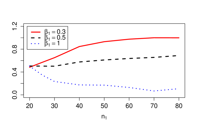
Figure 2: Simulated power for the models in (5.1) for different values of $\beta_{1}$ as a function of the sample size $n_{1}$ in the time domain.

Due to very high computational costs the sample size $n_{1}$ only varies between $20$ and $80$. We see that the curves indeed confirm what is predicted by the theory: For $\beta_{1}<1/2$ the power increases towards one and for $\beta_{1}>1/2$ it decreases towards the type one error rate of $\alpha=5\%$. For $\beta_{1}=1/2$ one could assume that the power increases as well when looking at Figure 2; Table 4 shows, however, that for larger sample sizes in the time domain it levels off between 0.7 and 0.8 which thus confirms the theory as well.

$n_{1}$	$80$	$160$	$240$	$320$
$\beta_{1}=0.5$	0.689	0.760	0.778	0.786

Table 4: Simulated power for the models in (5.1) for $\beta_{1}=0.5$ and different sample sizes $n_{1}$.

Appendix A Proofs

A.1 Preliminaries

Before proving the main results of this paper we briefly want to review the Skorohod space for functions defined on $[0,1]^{q}$ as well as the multivariate Riemann-Stieltjes integral.

The functional $\mathcal{F}_{n}(s,t,r_{2},r_{3})$ and its variations that were introduced in the previous sections can be viewed as an element of the Skorohod space $D_{q}=D[0,1]^{q}$ for functions defined on $[0,1]^{q}$ with $q\in\mathbb{N}$. This function space is the generalisation of the well-known Skorohod space $D=D[0,1]$ for functions with a single time parameter to functions with several time parameters and thus allows for certain discontinuities.

Informally speaking, the space $D[0,1]^{q}$ contains all real-valued functions that are ‘continuous from above, with limits from below’. To be more precise, let $\bm{t}\in[0,1]^{q}$ and define $R_{p}$, for all $1\leq p\leq q$, as one of the relations ‘$<$’ and ‘$\geq$’. Denote by $Q_{R_{1},\ldots,R_{q}}(\bm{t})$ the quadrant

$$\{(s_{1},\ldots,s_{q})\in[0,1]^{q}:s_{p}R_{p}t_{p},1\leq p\leq q\}.$$

We say that $f$ is an element of $D_{q}$ if the following two conditions hold:

• The limit

  $$f_{Q}\coloneqq\lim_{\bm{s}\to\bm{t},\atop\bm{s}\in Q}f(\bm{s})$$

  exists for each of the $2^{q}$ quadrants $Q=Q_{R_{1},\ldots,R_{q}}(\bm{t})$.

• We have

  $$f(\bm{t})=f_{Q_{\geq,\ldots,\geq}}=\lim_{\bm{s}\to\bm{t}\atop\bm{s}\in Q_{\geq,\ldots,\geq}}f(\bm{s}).$$

These conditions are analogously to the ones for $D[0,1]$. For more details, including the notion of weak convergence in $D[0,1]^{q}$, we refer to Straf (1972) and Bickel and Wichura (1971) respectively.

The generalization of the univariate Riemann-Stieltjes integral to the multivariate Riemann-Stieltjes integral in $q$ dimensions is now done by means of the $q$-fold alternating sum of a function in (3.1), cf. also Sard (1963).

Let $\mathcal{Y}=\prod_{j=1}^{q}\mathcal{Y}_{j}$ be a ladder on the hyperrectangle $[\bm{a},\bm{b}]\subset\mathbb{R}^{q}$, where $\mathcal{Y}_{j}$ is a ladder on $\left[a_{j},b_{j}\right]$ for all $j=1,\ldots,q$. Let $\widetilde{\bm{y}}\in\left[\bm{y},\bm{y}^{+}\right]$ for each $\bm{y}\in\mathcal{Y}$, where $\bm{y}^{+}$ denotes the component-by-component successor of $\bm{y}$, see above. Define a norm $\|\mathcal{Y}\|$ on $[\bm{a},\bm{b}]$ as

$$\left\|\mathcal{Y}\right\|\coloneqq\max\left\{\max_{y_{1}\in\mathcal{Y}_{1}}\left(y_{1}^{+}-y_{1}\right),\max_{y_{2}\in\mathcal{Y}_{2}}\left(y_{2}^{+}-y_{2}\right),\ldots,\max_{y_{q}\in\mathcal{Y}_{q}}\left(y_{q}^{+}-y_{q}\right)\right\}.$$

Suppose that $f$ and $h$ are real-valued functions defined on the hyperrectangle $[\bm{a},\bm{b}]$. Now, for each ladder $\mathcal{Y}\in\mathbb{Y}=\prod_{j=1}^{q}\mathbb{Y}_{j}$ consider the so-called Riemann-Stieltjes sum

$$\Sigma\coloneqq\sum_{\bm{y}\in\mathcal{Y}}h\left(\widetilde{\bm{y}}\right)\Delta\left(f;\bm{y},\bm{y}_{+}\right)=\sum_{\bm{y}\in\mathcal{Y}}h\left(\widetilde{\bm{y}}\right)\left[\sum_{v\subseteq\{1,\ldots,q\}}(-1)^{|v|}f\left(\bm{y}_{v}:\bm{y}^{+}_{-v}\right)\right].$$ (A.1)

Analogously to the one-dimensional case we now define the Riemann-Stieltjes integral of $h$ with respect to $f$ as

$$\int_{\bm{a}}^{\bm{b}}\!h(\bm{x})\,\mathrm{d}f(\bm{x})\coloneqq\lim_{\left\|\mathcal{Y}\right\|\to 0}\Sigma,$$ (A.2)

if the latter exists. The integral on the left is understood as a multivariate integral, namely as

$$\int_{\bm{a}}^{\bm{b}}\!h(\bm{x})\,\mathrm{d}f(\bm{x}) =\int_{\bm{a}_{1:q}}^{\bm{b}_{1:q}}\!h(\bm{x})\,\mathrm{d}f\left(\bm{x}\right)$$

$$=\int_{a_{1}}^{b_{1}}\int_{a_{2}}^{b_{2}}\ldots\int_{a_{q}}^{b_{q}}\!h\left(x_{1},x_{2},\ldots,x_{q}\right)\,\mathrm{d}f\left(x_{1},x_{2},\ldots,x_{q}\right).$$

Similar to the one-dimensional case this integral and all ‘lower dimensional’ integrals exist if $h$ is a continuous function on the hyperrectangle $[\bm{a},\bm{b}]$, $\bm{a},\bm{b}\in\mathbb{R}^{q}$ and if $f$ is a function of bounded variation in the sense of Hardy and Krause on $[\bm{a},\bm{b}]$.

Moreover, there exists a generalization of the integration by parts formula for multivariate Riemann-Stieltjes integrals, see Young (1917), p. 287. This allows us to define the multivariate Riemann-Stieltjes integral even with respect to functions $h$ that are not of bounded variation in the sense of Vitali or in the sense of Hardy and Krause. In this case we take the integration by parts formula as a definition for the integral, i.e. we put

$$\int_{\bm{a}_{1:q}}^{\bm{b}_{1:q}}\!f(\bm{x})\,\mathrm{d}h(\bm{x}) \coloneqq\left[h(\bm{x})f(\bm{x})\right]_{\bm{a}_{1:q}}^{\bm{b}_{1:q}}+(-1)^{q}\int_{\bm{a}_{1:q}}^{\bm{b}_{1:q}}\!h(\bm{x})\,\mathrm{d}f(\bm{x})$$

$$+\sum_{v\subseteq\{1,\ldots,q\},\atop 1\leq|v|\leq q-1}(-1)^{|v|}\int_{\bm{a}_{v}}^{\bm{b}_{v}}\!\left[h(\bm{x})\,\mathrm{d}f(\bm{x})\right]_{\bm{a}_{-v}}^{\bm{b}_{-v}}$$ (A.3)

whenever the right-hand side exists. The square bracket notation is used for the evaluation, respectively, the increment of a multivariate antiderivative $f$ over a hyperrectangle $[\bm{a},\bm{b}]\subset\mathbb{R}^{q}$. Thus, we have

$$\left[f(\bm{x})\right]_{\bm{a}}^{\bm{b}}=\left[f(x_{1},\ldots,x_{q})\right]_{\bm{a}_{1:q}}^{\bm{b}_{1:q}}\coloneqq\Delta(f;\bm{a},\bm{b})=\sum_{v\subseteq\{1,\ldots,q\}}(-1)^{|v|}f\left(\bm{a}_{v}:\bm{b}_{-v}\right).$$

If the evaluation of $f$ only takes place over a hyperrectangle $\left[\bm{a}_{-v},\bm{b}_{-v}\right],\ v\subset 1:q$, we write $\left[f(\bm{x})\right]_{\bm{a}_{-v}}^{\bm{b}_{-v}}$, and this is defined as

$$\left[f(\bm{x})\right]_{\bm{a}_{-v}}^{\bm{b}_{-v}}=\left[f\left(\bm{x}_{v}:\bm{x}_{-v}\right)\right]_{\bm{a}_{-v}}^{\bm{b}_{-v}}\coloneqq\sum_{w\subseteq-v}(-1)^{|w|}f\left(\bm{x}_{v}:\bm{a}_{w}:\bm{b}_{-w}\right).$$

Thus, we can define the Riemann-Stieltjes integral with respect to a (multivariable) Brownian motion, where the sample paths are of unbounded variation almost surely.

A.2 Proofs

This section is devoted to rigorous proofs of the presented theorems. Note that parts of the material are taken from Prause (2015). We start with proving Theorem 3.1 and introduce the following abbreviating notation. Let

$$\varphi_{w}(v_{1},v_{2},v_{3},t,r_{2},r_{3})\coloneqq\varphi\left(t-\overline{\tau}_{1}v_{1},r_{2}-\overline{\tau}_{2}v_{2},r_{3}-\overline{\tau}_{3}v_{3}\right)$$ (A.4)

for $v_{1},v_{2},v_{3}\in[0,1]$, $t\in[0,\overline{\tau}_{1}]$, $r_{2}\in[0,\overline{\tau}_{2}]$ and $r_{3}\in[0,\overline{\tau}_{3}]$. Here,

$$\quad\ \ \varphi\left(t-\overline{\tau}_{1}v_{1},r_{2}-\overline{\tau}_{2}v_{2},r_{3}-\overline{\tau}_{3}v_{3}\right)$$

$$\hskip 56.9055pt=\frac{\sin(\Omega_{1}(t-\overline{\tau}_{1}v_{1}))}{\pi(t-\overline{\tau}_{1}v_{1})}\frac{\sin(\Omega_{2}(r_{2}-\overline{\tau}_{2}v_{2}))}{\pi(r_{2}-\overline{\tau}_{2}v_{2})}\frac{\sin(\Omega_{3}(r_{3}-\overline{\tau}_{3}v_{3}))}{\pi(r_{3}-\overline{\tau}_{3}v_{3})}$$

$$\hskip 56.9055pt\eqqcolon\varphi_{1}(v_{1},t)\varphi_{2}(v_{2},r_{2})\varphi_{3}(v_{3},r_{3})$$

with $\varphi_{j}(v_{j},\overline{\tau}_{j}v_{j})=\Omega_{j}/\pi$ for $j=1,2,3$.

For the proof of Theorem 3.1 we need the following lemmas.

Lemma A.1.

Let $\varphi_{w}$ be defined as in (A.4). Then

$$\sup_{t\in[0,\overline{\tau}_{1}],\atop{r_{2}\in[0,\overline{\tau}_{2}],r_{3}\in[0,\overline{\tau}_{3}]}}V_{HK}(\varphi_{w}(\cdot,\cdot,\cdot,t,r_{2},r_{3}))<\infty.$$

Proof..

By Proposition 11 in Owen (2005) we know that for $f,g\in\$BVHK we also have $fg\in\$BVHK; thus, we can consider each factor of $\varphi_{w}$ separately and the assertion follows by the one-dimensional theory for functions of bounded variation. ∎

Lemma A.2.

Let $h$ be a real-valued function on $[\bm{a},\bm{b}]$ and let $f$ be a function of bounded variation in the sense of Hardy and Krause on $[\bm{a},\bm{b}]$. Suppose that

$$\int_{\bm{a}_{v}}^{\bm{b}_{v}}\!\left[f(\bm{x})\,\mathrm{d}h(\bm{x})\right]_{\bm{a}_{-v}}^{\bm{b}_{-v}}$$

exists for all $\emptyset\neq v\subseteq 1:q$. Then there exists a constant $c\in\mathbb{R}$ such that

$$\left|\int_{\bm{a}}^{\bm{b}}\!f(\bm{x})\,\mathrm{d}h(\bm{x})\right|\leq 2^{q}\sup_{\bm{x}\in[\bm{a},\bm{b}]}|h(\bm{x})|\left[\sup_{\bm{x}\in[\bm{a},\bm{b}]}|f(\bm{x})|+cV_{HK}(f)\right].$$ (A.5)

Proof..

The assertion follows by an application of the integration by parts formula combined with the definition of the multivariate Riemann-Stieltjes integral and the variation in the sense of Hardy and Krause. ∎

Lemma A.3.

Let $\bm{a},\bm{b}\in\mathbb{R}^{q}$, $\widetilde{\bm{a}},\widetilde{\bm{b}}\in\mathbb{R}^{p}$ with $\bm{a}\leq\bm{b},\widetilde{\bm{a}}\leq\widetilde{\bm{b}}$, $p,q\in\mathbb{N}$. Let $\psi$ be a bounded function on $[\bm{a},\bm{b}]\times[\widetilde{\bm{a}},\widetilde{\bm{b}}]$ with

$$\sup_{\bm{y}\in[\widetilde{\bm{a}},\widetilde{\bm{b}}]}V_{HK}\left(\psi(\bm{\cdot},\bm{y})\right)<\infty.$$

Let $\{f_{n}\}$ be a sequence of functions such that $f_{n}\in D[\bm{a},\bm{b}]$ for all $n\in\mathbb{N}$. Suppose that $\lim_{n\to\infty}f_{n}=f$ in the Skorohod topology for a function $f\in C[\bm{a},\bm{b}]$. Moreover, suppose that

$$\int_{\bm{a}_{v}}^{\bm{s}_{v}}\!\left[\psi(\bm{x},\bm{y})\,\mathrm{d}f_{n}(\bm{x})\right]_{\bm{a}_{-v}}^{\bm{s}_{-v}}$$

exists for $\bm{s}_{v}\in[\bm{a}_{v},\bm{b}_{v}]$, $\bm{y}\in[\widetilde{\bm{a}},\widetilde{\bm{b}}]$ and for all $n\in\mathbb{N}$ and $\emptyset\neq v\subseteq 1:q$. Then,

$$\lim_{n\to\infty}\sup_{\bm{s}\in[\bm{a},\bm{b}]}\sup_{\bm{y}\in[\widetilde{\bm{a}},\widetilde{\bm{b}}]}\left|\int_{\bm{a}}^{\bm{s}}\!\psi(\bm{x},\bm{y})\,\mathrm{d}f_{n}(\bm{x})-\int_{\bm{a}}^{\bm{s}}\!\psi(\bm{x},\bm{y})\,\mathrm{d}f(\bm{x})\right|=0.$$

Proof..

An application of Lemma A.2 and the fact that Skorohod convergence towards a continuous limit implies uniform convergence show the assertion. ∎

We now prove Theorem 3.1. To simplify the notation we put $n=n_{1}=n_{2}=n_{3}$, but the proof can be completed along the same lines if the $n_{i},i=1,2,3,$ differ.

Proof of Theorem 3.1.

We consider the function space $D[0,1]^{3}$ and define the functional

$$\Lambda(f)=\Lambda(f)(s,t,r_{2},r_{3})\coloneqq\sqrt{\overline{\tau}_{1}\overline{\tau}_{2}\overline{\tau}_{3}}\int_{0}^{s}\int_{0}^{1}\int_{0}^{1}\!\varphi_{w}(v_{1},v_{2},v_{3},t,r_{2},r_{3})\,\mathrm{d}f(v_{1},v_{2},v_{3})$$

for $0<s_{0}\leq s\leq 1$, $t\in[0,\overline{\tau}_{1}]$, $r_{2}\in[0,\overline{\tau}_{2}]$, and $r_{3}\in[0,\overline{\tau}_{3}]$ on it, whenever the integral exists. Here $\varphi_{w}$ is defined as in (A.4). Let $\{f_{n}\}$ be a sequence of functions such that $f_{n}\in D[0,1]^{3}$ for all $n\in\mathbb{N}$. We know by Lemma A.3, that $\lim_{n\to\infty}f_{n}=f$ in the Skorohod topology with $f\in C[0,1]^{3}$ implies

$$\sup_{s\in[s_{0},1]}\sup_{t\in[0,\overline{\tau}_{1}],\atop r_{2}\in[0,\overline{\tau}_{2}],r_{3}\in[0,\overline{\tau}_{3}]}\left|\int_{0}^{s}\int_{0}^{1}\int_{0}^{1}\!\varphi_{w}(v_{1},v_{2},v_{3},t,r_{2},r_{3})\,\mathrm{d}f_{n}(v_{1},v_{2},v_{3})\right.$$

$$\left.\hskip 99.58464pt-\int_{0}^{s}\int_{0}^{1}\int_{0}^{1}\!\varphi_{w}(v_{1},v_{2},v_{3},t,r_{2},r_{3})\,\mathrm{d}f(v_{1},v_{2},v_{3})\right|\to 0$$ (A.6)

in $D([s_{0},1]\times[0,\overline{\tau}_{1}]\times[0,\overline{\tau}_{2}]\times[0,\overline{\tau}_{3}])$ as $n\to\infty$, since

$$\sup_{t\in[0,\overline{\tau}_{1}],\atop{r_{2}\in[0,\overline{\tau}_{2}],r_{3}\in[0,\overline{\tau}_{3}]}}V_{HK}(\varphi_{w}(\cdot,\cdot,\cdot,t,r_{2},r_{3}))<\infty$$

by Lemma A.1. Assumption 1 and the continuous mapping theorem now lead to

$$\Lambda(Z_{n}(\cdot)) =\sqrt{\overline{\tau}_{1}\overline{\tau}_{2}\overline{\tau}_{3}}\int_{0}^{s}\int_{0}^{1}\int_{0}^{1}\!\varphi_{w}(v_{1},v_{2},v_{3},t,r_{2},r_{3})\,\mathrm{d}Z_{n}(v_{1},v_{2},v_{3})$$

$$\Rightarrow\sqrt{\overline{\tau}_{1}\overline{\tau}_{2}\overline{\tau}_{3}}\,\sigma\int_{0}^{s}\int_{0}^{1}\int_{0}^{1}\!\varphi_{w}(v_{1},v_{2},v_{3},t,r_{2},r_{3})\,\mathrm{d}B(v_{1},v_{2},v_{3}),$$

as $n\to\infty$, since $P(B(v_{1},v_{2},v_{3})\in C\left([0,1]^{3}\right))=1$.

On the other hand we have

$$\Lambda(Z_{n}(\cdot))=\sqrt{\frac{\overline{\tau}_{1}\overline{\tau}_{2}\overline{\tau}_{3}}{n^{3}}}\int_{0}^{s}\int_{0}^{1}\int_{0}^{1}\!\varphi_{w}(v_{1},v_{2},v_{3},t,r_{2},r_{3})\,\mathrm{d}\left(\sum_{i_{1}=1}^{\lfloor nv_{1}\rfloor}\sum_{i_{2}=1}^{\lfloor nv_{2}\rfloor}\sum_{i_{3}=1}^{\lfloor nv_{3}\rfloor}\varepsilon_{i_{1},i_{2},i_{3}}\right).$$ (A.7)

We now interpret this last integral as a multivariate Riemann-Stieltjes integral. Let $\mathcal{Y}_{1}$ be a ladder on $[0,s]$ for $s\in[s_{0},1]$ and let $\mathcal{Y}_{2}$ and $\mathcal{Y}_{3}$ be ladders on $[0,1]$. Then we can write the triple integral as

$$\quad\int_{0}^{s}\int_{0}^{1}\int_{0}^{1}\!\varphi_{w}(v_{1},v_{2},v_{3},t,r_{2},r_{3})\,\mathrm{d}\left(\sum_{i_{1}=1}^{\lfloor nv_{1}\rfloor}\sum_{i_{2}=1}^{\lfloor nv_{2}\rfloor}\sum_{i_{3}=1}^{\lfloor nv_{3}\rfloor}\varepsilon_{i_{1},i_{2},i_{3}}\right)$$

$$=\lim_{\left\|\mathcal{Y}\right\|\to 0}\sum_{\bm{y}\in\mathcal{Y}}\varphi_{w}(\widetilde{y}_{1},\widetilde{y}_{2},\widetilde{y}_{3},t,r_{2},r_{3})$$

$$\hskip 62.59596pt\left[\sum_{i_{1}=1}^{\lfloor ny^{+}_{1}\rfloor}\sum_{i_{2}=1}^{\lfloor ny^{+}_{2}\rfloor}\sum_{i_{3}=1}^{\lfloor ny^{+}_{3}\rfloor}\varepsilon_{i_{1},i_{2},i_{3}}-\sum_{i_{1}=1}^{\lfloor ny_{1}\rfloor}\sum_{i_{2}=1}^{\lfloor ny^{+}_{2}\rfloor}\sum_{i_{3}=1}^{\lfloor ny^{+}_{3}\rfloor}\varepsilon_{i_{1},i_{2},i_{3}}\right.$$

$$\left.\hskip 62.59596pt-\sum_{i_{1}=1}^{\lfloor ny^{+}_{1}\rfloor}\sum_{i_{2}=1}^{\lfloor ny_{2}\rfloor}\sum_{i_{3}=1}^{\lfloor ny^{+}_{3}\rfloor}\varepsilon_{i_{1},i_{2},i_{3}}-\sum_{i_{1}=1}^{\lfloor ny^{+}_{1}\rfloor}\sum_{i_{2}=1}^{\lfloor ny^{+}_{2}\rfloor}\sum_{i_{3}=1}^{\lfloor ny_{3}\rfloor}\varepsilon_{i_{1},i_{2},i_{3}}\right.$$

$$\left.\hskip 62.59596pt+\sum_{i_{1}=1}^{\lfloor ny_{1}\rfloor}\sum_{i_{2}=1}^{\lfloor ny_{2}\rfloor}\sum_{i_{3}=1}^{\lfloor ny^{+}_{3}\rfloor}\varepsilon_{i_{1},i_{2},i_{3}}+\sum_{i_{1}=1}^{\lfloor ny_{1}\rfloor}\sum_{i_{2}=1}^{\lfloor ny^{+}_{2}\rfloor}\sum_{i_{3}=1}^{\lfloor ny_{3}\rfloor}\varepsilon_{i_{1},i_{2},i_{3}}\right.$$

$$\left.\hskip 62.59596pt+\sum_{i_{1}=1}^{\lfloor ny^{+}_{1}\rfloor}\sum_{i_{2}=1}^{\lfloor ny_{2}\rfloor}\sum_{i_{3}=1}^{\lfloor ny_{3}\rfloor}\varepsilon_{i_{1},i_{2},i_{3}}-\sum_{i_{1}=1}^{\lfloor ny_{1}\rfloor}\sum_{i_{2}=1}^{\lfloor ny_{2}\rfloor}\sum_{i_{3}=1}^{\lfloor ny_{3}\rfloor}\varepsilon_{i_{1},i_{2},i_{3}}\right],$$

where $\bm{y}_{+}=\left(y^{+}_{1},y^{+}_{2},y^{+}_{3}\right)$ is the component-by-component successor of the point $\bm{y}=\left(y_{1},y_{2},y_{3}\right)$, $\widetilde{\bm{y}}=\left(\widetilde{y}^{1},\widetilde{y}^{2},\widetilde{y}^{3}\right)$ is an arbitrary point in the cube $[\bm{y},\bm{y}_{+}]$ and

$$\left\|\mathcal{Y}\right\|=\max\left\{\max_{y_{1}\in\mathcal{Y}_{1}}(y^{+}_{1}-y_{1}),\max_{y_{2}\in\mathcal{Y}_{2}}(y^{+}_{2}-y_{2}),\max_{y_{3}\in\mathcal{Y}_{3}}(y^{+}_{3}-y_{3})\right\}.$$

Consider now, without loss of generality, a ladder $\mathcal{Y}=\prod_{i=1}^{3}\mathcal{Y}_{i}$ with $y_{i}<k_{i}/n\leq y^{+}_{i}$ for all $k_{1}\in\{1,\ldots,\left\lfloor ns\right\rfloor\}$ and all $k_{2},k_{3}\in\{1,\ldots,n\}$, respectively, and write $\widetilde{y}_{k_{i}}$ for points $\widetilde{y}_{k_{i}}\in(y_{i},y_{i}^{+}],i=1,2,3$. As the floor function $\lfloor ny\rfloor$ is constant on intervals of the form $\left[(k-1)/n,k/n\right)$, $k\in\{1,\ldots,n\}$, the triple sums in the last expression can be combined and we obtain

$$\quad\sum_{i_{1}=1}^{\lfloor ny^{+}_{1}\rfloor}\sum_{i_{2}=1}^{\lfloor ny^{+}_{2}\rfloor}\varepsilon_{i_{1},i_{2},k_{3}}-\sum_{i_{1}=1}^{\lfloor ny^{+}_{1}\rfloor}\sum_{i_{2}=1}^{\lfloor ny_{2}\rfloor}\varepsilon_{i_{1},i_{2},k_{3}}-\sum_{i_{1}=1}^{\lfloor ny_{1}\rfloor}\sum_{i_{2}=1}^{\lfloor ny^{+}_{2}\rfloor}\varepsilon_{i_{1},i_{2},k_{3}}+\sum_{i_{1}=1}^{\lfloor ny_{1}\rfloor}\sum_{i_{2}=1}^{\lfloor ny_{2}\rfloor}\varepsilon_{i_{1},i_{2},k_{3}}$$

$$=\sum_{i_{1}=1}^{\lfloor ny^{+}_{1}\rfloor}\varepsilon_{i_{1},k_{2},k_{3}}-\sum_{i_{1}=1}^{\lfloor ny_{1}\rfloor}\varepsilon_{i_{1},k_{2},k_{3}}=\varepsilon_{k_{1},k_{2},k_{3}}.$$

This leads to

$$\quad\int_{0}^{s}\int_{0}^{1}\int_{0}^{1}\!\varphi_{w}(v_{1},v_{2},v_{3},t,r_{2},r_{3})\,\mathrm{d}\left(\sum_{i_{1}=1}^{\lfloor nv_{1}\rfloor}\sum_{i_{2}=1}^{\lfloor nv_{2}\rfloor}\sum_{i_{3}=1}^{\lfloor nv_{3}\rfloor}\varepsilon_{i_{1},i_{2},i_{3}}\right)$$

$$=\lim_{\left\|P\right\|\to 0}\sum_{k_{1}=1}^{\lfloor ns\rfloor}\sum_{k_{2}=1}^{n}\sum_{k_{3}=1}^{n}\varphi_{w}(\widetilde{y}_{k_{1}},\widetilde{y}_{k_{2}},\widetilde{y}_{k_{3}},t,r_{2},r_{3})\varepsilon_{k_{1},k_{2},k_{3}}$$

$$=\sum_{k_{1}=1}^{\lfloor ns\rfloor}\sum_{k_{2}=1}^{n}\sum_{k_{3}=1}^{n}\varphi_{w}\left(\frac{k_{1}}{n},\frac{k_{2}}{n},\frac{k_{3}}{n},t,r_{2},r_{3}\right)\varepsilon_{k_{1},k_{2},k_{3}},$$

where the last equality holds as

$$\left\|\left(\widetilde{y}_{k_{1}},\widetilde{y}_{k_{2}},\widetilde{y}_{k_{3}}\right)^{\prime}-\left(\frac{k_{1}}{n},\frac{k_{2}}{n},\frac{k_{3}}{n}\right)^{\prime}\right\| \leq\left\|\left(y^{+}_{1}-y_{1},y^{+}_{2}-y_{2},y^{+}_{3}-y_{3}\right)^{\prime}\right\|$$

$$\leq\left\|\mathcal{Y}\right\|\to 0.$$

Now we can write (A.7) as

$$\Lambda(Z_{n}(\cdot)) =\sqrt{\frac{\overline{\tau}_{1}\overline{\tau}_{2}\overline{\tau}_{3}}{n^{3}}}\sum_{k_{1}=1}^{\lfloor ns\rfloor}\sum_{k_{2}=1}^{n}\sum_{k_{3}=1}^{n}\varphi_{w}\left(\frac{k_{1}}{n},\frac{k_{2}}{n},\frac{k_{3}}{n},t,r_{2},r_{3}\right)\varepsilon_{k_{1},k_{2},k_{3}}.$$

If we recall the definition of $\varphi_{w}$ from (A.4) and the fact that $\tau_{j}\approx\overline{\tau}_{j}/n$, $j=1,2,3$, we obtain that

$$\mathcal{F}_{n}(s,t,r_{2},r_{3})=\Lambda(Z_{n}(\cdot))+o_{P}(1).$$

This completes the proof. ∎

Proof of Lemma 3.1.

The proof of this lemma is omitted here as it is analogously to the proof of Corollary 1 in Pawlak and Steland (2013), since the properties in Theorem 5.1.4 in Ash and Gardner (1975) also hold true for multivariate Riemann-Stieltjes integrals. ∎

Proof of Lemma 3.2.

The assertion directly follows with Theorem 3.1 and the continuous mapping theorem. ∎

Before we prove Theorem 3.2 we review the Hwlaka-Koksma inequality which gives an error bound for the discrete approximation of a Riemann integral for functions of bounded variation in the sense of Hardy and Krause, see for example Niederreiter (1992), Theorem 2.11. For this we need the notion of discrepancy which measures the deviation of an arbitrary point set in the unit cube from a uniformly distributed point set. Hence, let $P$ be a point set consisting of $\bm{x}^{(1)},\ldots,\bm{x}^{(N)}\in[0,1]^{q}$. Now, for an arbitrary subset $B$ of $[0,1]^{q}$, we define

$$A(B;P)\coloneqq\sum_{i=1}^{N}\bm{1}_{B}\left(\bm{x}^{(i)}\right),$$

i.e. $A(B;P)$ counts the number of points of $\bm{x}^{(1)},\ldots,\bm{x}^{(N)}$ lying in $B$. We then define the general discrepancy of the point set $P$ for a nonempty family $\mathcal{B}$ of Lebesgue-measurable subsets of $[0,1]^{q}$ as

$$D_{N}(B;P)\coloneqq\sup_{B\in\mathcal{B}}\left|\frac{A(B;P)}{N}-\lambda_{q}(B)\right|.$$

This leads to the following notion of discrepancy, cf. Definition 2.1. in Niederreiter (1992).

Definition A.1.

The star discrepancy $D_{N}^{\star}(P)=D_{N}^{\star}\left(\bm{x}^{(1)},\ldots,\bm{x}^{(N)}\right)$ of the point set $P$ is defined by $D_{N}^{\star}(P)\coloneqq D_{N}(\mathcal{J}^{\star};P)$, where $\mathcal{J}^{\star}$ is the family of all subintervals of $[0,1]^{q}$ of the form $\prod_{i=1}^{q}[0,u_{i})$.

We can now state the well-known Hwlaka-Koksma inequality for multivariable functions.

Lemma A.4.

If $f$ has bounded variation $V_{HK}(f)$ on $[0,1]^{q}$ in the sense of Hardy and Krause, then, for any $\bm{x}^{(1)},\ldots,\bm{x}^{(N)}\in[0,1]^{q}$, we have

$$\left|\frac{1}{N}\sum_{i=1}^{N}f\left(\bm{x}^{(i)}\right)-\int_{[0,1]^{q}}\!f(\bm{u})\,\mathrm{d}\bm{u}\right|\leq V_{HK}(f)D_{N}^{\star}\left(\bm{x}^{(1)},\ldots,\bm{x}^{(N)}\right).$$

We now prove Theorem 3.2. To simplify the notation we put again $n=n_{1}=n_{2}=n_{3}$, but the proof can be completed along the same lines if the $n_{i},i=1,2,3,$ differ.

Proof of Theorem 3.2.

The local alternative is given by

$$y_{k_{1},k_{2},k_{3}}=f_{n}\left(k_{1}\tau_{1},k_{2}\tau_{2},k_{3}\tau_{3}\right)+\varepsilon_{k_{1},k_{2},k_{3}}$$

with

$$f_{n}(t,r_{2},r_{3})=f_{0}(t,r_{2},r_{3})+\frac{\delta(t,r_{2},r_{3})}{n^{\beta}}$$

for $\beta>0$. Our test statistic $\mathcal{F}_{n}(s,t,r_{2},r_{3})$ is therefore defined as

$$\mathcal{F}_{n}(s,t,r_{2},r_{3}) =\sqrt{\tau_{1}\tau_{2}\tau_{3}}\sum_{l_{1}=1}^{\lfloor ns\rfloor}\sum_{l_{2}=1}^{n}\sum_{l_{3}=1}^{n}\varepsilon_{k_{1},k_{2},k_{3}}\varphi\left(t-k_{1}\tau_{1},r_{2}-k_{2}\tau_{2},r_{3}-k_{3}\tau_{3}\right)$$

$$+\frac{\sqrt{\tau_{1}\tau_{2}\tau_{3}}}{n^{\beta}}\sum_{l_{1}=1}^{\lfloor ns\rfloor}\sum_{l_{2}=1}^{n}\sum_{l_{3}=1}^{n}\delta(k_{1}\tau_{1},k_{2}\tau_{2},k_{3}\tau_{3})$$

$$\hskip 116.65646pt\varphi\left(t-k_{1}\tau_{1},r_{2}-k_{2}\tau_{2},r_{3}-k_{3}\tau_{3}\right)$$

$$\eqqcolon T_{n}^{(1)}(s,t,r_{2},r_{3})+T_{n}^{(2)}(s,t,r_{2},r_{3}).$$

$T_{n}^{(1)}(s,t,r_{2},r_{3})$ equals $\mathcal{F}_{n}(s,t,r_{2},r_{3})$ under the null hypothesis which converges to the process $\mathcal{F}(s,t,r_{2},r_{3})$ of Theorem 3.1 for $n\to\infty$.

By assumption on the sampling periods we obtain for the second process

$$T_{n}^{(2)}(s,t,r_{2},r_{3})=\frac{1}{n^{\beta-3/2}}\frac{1}{\sqrt{\overline{\tau}_{1}\overline{\tau}_{2}\overline{\tau}_{3}}}\frac{\overline{\tau}_{1}\overline{\tau}_{2}\overline{\tau}_{3}}{n^{3}}$$

$$\qquad\sum_{k_{1}=1}^{\lfloor ns\rfloor}\sum_{k_{2}=1}^{n}\sum_{k_{3}=1}^{n}\delta\left(k_{1}\frac{\overline{\tau}_{1}}{n},k_{2}\frac{\overline{\tau}_{2}}{n},k_{3}\frac{\overline{\tau}_{3}}{n}\right)\varphi\left(t-k_{1}\frac{\overline{\tau}_{1}}{n},r_{2}-k_{2}\frac{\overline{\tau}_{2}}{n},r_{3}-k_{3}\frac{\overline{\tau}_{3}}{n}\right)+o(1).$$

We now fix $\beta=3/2$ and set

$$\varphi_{\delta}(t,r_{2},r_{3},z_{1},z_{2},z_{3})=\delta(z_{1},z_{2},z_{3})\varphi(t-z_{1},r_{2}-z_{2},r_{3}-z_{3}).$$

If we can show that

$$\sup_{s\in[s_{0},1]}\sup_{t\in[0,\overline{\tau}_{1}],\atop r_{2}\in[0,\overline{\tau}_{2}],r_{3}\in[0,\overline{\tau}_{3}]}\left|\frac{\overline{\tau}_{1}\overline{\tau}_{2}\overline{\tau}_{3}}{n^{3}}\sum_{k_{1}=1}^{\lfloor ns\rfloor}\sum_{k_{2}=1}^{n}\sum_{k_{3}=1}^{n}\varphi_{\delta}\left(t,r_{2},r_{3},k_{1}\frac{\overline{\tau}_{1}}{n},k_{2}\frac{\overline{\tau}_{2}}{n},k_{3}\frac{\overline{\tau}_{3}}{n}\right)\right.$$

$$\left.\hskip 116.65646pt-\int_{0}^{s\overline{\tau}_{1}}\int_{0}^{\overline{\tau}_{2}}\int_{0}^{\overline{\tau}_{3}}\!\varphi_{\delta}\left(t,r_{2},r_{3},z_{1},z_{2},z_{3}\right)\,\mathrm{d}z_{3}\mathrm{d}z_{2}\mathrm{d}z_{1}\right|$$ (A.8)

tends to zero as $n\to\infty$ the assertion follows, since uniform convergence always implies convergence in the Skorohod topology.

If $\delta(t,r_{2},r_{3})$ is continuous we can proceed in an analogous way as in the proof of Theorem 3 of Pawlak and Steland (2013). Thus, it remains to treat the case that $\delta(t,r_{2},r_{3})$ is of bounded variation in the sense of Hardy and Krause. Our aim is to apply the Hwlaka-Koksma inequality of Lemma A.4. As this inequality is formulated for integrals over the unit cube we first observe that

$$\int_{0}^{s\overline{\tau}_{1}}\int_{0}^{\overline{\tau}_{2}}\int_{0}^{\overline{\tau}_{2}}\!\varphi_{\delta}\left(t,r_{2},r_{3},z_{1},z_{2},z_{3}\right)\,\mathrm{d}z_{3}\mathrm{d}z_{2}\mathrm{d}z_{1}$$

$$\qquad=\int_{0}^{1}\int_{0}^{1}\int_{0}^{1}\!s\overline{\tau}_{1}\overline{\tau}_{2}\overline{\tau}_{3}\varphi_{\delta}\left(t,r_{2},r_{3},s\overline{\tau}_{1}z_{1},\overline{\tau}_{2}z_{2},\overline{\tau}_{3}z_{3}\right)\,\mathrm{d}z_{3}\mathrm{d}z_{2}\mathrm{d}z_{1}.$$

Put $\left(x_{k_{1}},x_{k_{2}},x_{k_{3}}\right)=\left(\frac{k_{1}\overline{\tau}_{1}}{n},\frac{k_{2}\overline{\tau}_{2}}{n},\frac{k_{3}\overline{\tau}_{3}}{n}\right)$ and $\left(\widetilde{x}_{k_{1}},\widetilde{x}_{k_{2}},\widetilde{x}_{k_{3}}\right)=\left(\frac{k_{1}}{ns},\frac{k_{2}}{n},\frac{k_{3}}{n}\right),$ for $\left(k_{1},k_{2},k_{3}\right)\in\{1,\ldots,\lfloor ns\rfloor\}\times\{1,\ldots,n\}\times\{1,\ldots,n\}$ and $s\geq s_{0}>0$. Then we obtain

$$\frac{\overline{\tau}_{1}\overline{\tau}_{2}\overline{\tau}_{3}}{n^{3}}\sum_{k_{1}=1}^{\lfloor ns\rfloor}\sum_{k_{2}=1}^{n}\sum_{k_{3}=1}^{n}\varphi_{\delta}\left(t,r_{2},r_{3},k_{1}\frac{\overline{\tau}_{1}}{n},k_{2}\frac{\overline{\tau}_{2}}{n},k_{3}\frac{\overline{\tau}_{3}}{n}\right)$$

$$\qquad=\frac{1}{sn^{3}}\sum_{k_{1}=1}^{\lfloor ns\rfloor}\sum_{k_{2}=1}^{n}\sum_{k_{3}=1}^{n}s\overline{\tau}_{1}\overline{\tau}_{2}\overline{\tau}_{3}\varphi_{\delta}\left(t,r_{2},r_{3},s\overline{\tau}_{1}\widetilde{x}_{k_{1}},\overline{\tau}_{2}\widetilde{x}_{k_{2}},\overline{\tau}_{3}\widetilde{x}_{k_{3}}\right).$$

Thus we can reformulate (A.2) as

$$\sup_{s\in[s_{0},1]}\sup_{t\in[0,\overline{\tau}_{1}],\atop r_{2}\in[0,\overline{\tau}_{2}],r_{3}\in[0,\overline{\tau}_{3}]}\left|\frac{1}{sn^{3}}\sum_{k_{1}=1}^{\lfloor ns\rfloor}\sum_{k_{2}=1}^{n}\sum_{k_{3}=1}^{n}s\overline{\tau}_{1}\overline{\tau}_{2}\overline{\tau}_{3}\varphi_{\delta}\left(t,r_{2},r_{3},s\overline{\tau}_{1}\widetilde{x}_{k_{1}},\overline{\tau}_{2}\widetilde{x}_{k_{2}},\overline{\tau}_{3}\widetilde{x}_{k_{3}}\right)\right.$$ (A.9)

$$\left.\hskip 113.81102pt-\int_{0}^{1}\int_{0}^{1}\int_{0}^{1}\!s\overline{\tau}_{1}\overline{\tau}_{2}\overline{\tau}_{3}\varphi_{\delta}\left(t,r_{2},r_{3},s\overline{\tau}_{1}z_{1},\overline{\tau}_{2}z_{2},\overline{\tau}_{3}z_{3}\right)\,\mathrm{d}z_{3}\mathrm{d}z_{2}\mathrm{d}z_{1}\right|.$$

An upper bound for this expression without the suprema is

$$\quad\ \left|\frac{1}{\lfloor ns\rfloor n^{2}}\sum_{k_{1}=1}^{\lfloor ns\rfloor}\sum_{k_{2}=1}^{n}\sum_{k_{3}=1}^{n}s\overline{\tau}_{1}\overline{\tau}_{2}\overline{\tau}_{3}\varphi_{\delta}\left(t,r_{2},r_{3},s\overline{\tau}_{1}\widetilde{x}_{k_{1}},\overline{\tau}_{2}\widetilde{x}_{k_{2}},\overline{\tau}_{3}\widetilde{x}_{k_{3}}\right)\right.$$

$$\left.-\int_{0}^{1}\int_{0}^{1}\int_{0}^{1}\!s\overline{\tau}_{1}\overline{\tau}_{2}\overline{\tau}_{3}\varphi_{\delta}\left(t,r_{2},r_{3},s\overline{\tau}_{1}z_{1},\overline{\tau}_{2}z_{2},\overline{\tau}_{3}z_{3}\right)\,\mathrm{d}z_{3}\mathrm{d}z_{2}\mathrm{d}z_{1}\right|$$

$$+\left|\left(\frac{1}{sn^{3}}-\frac{1}{\lfloor ns\rfloor n^{2}}\right)\sum_{k_{1}=1}^{\lfloor ns\rfloor}\sum_{k_{2}=1}^{n}\sum_{k_{3}=1}^{n}s\overline{\tau}_{1}\overline{\tau}_{2}\overline{\tau}_{3}\varphi_{\delta}\left(t,r_{2},r_{3},s\overline{\tau}_{1}\widetilde{x}_{k_{1}},\overline{\tau}_{2}\widetilde{x}_{k_{2}},\overline{\tau}_{3}\widetilde{x}_{k_{3}}\right)\right|$$

$$\eqqcolon S_{1}+S_{2}.$$

We first consider $S_{2}$. As both $\delta$ and $\varphi$ are of bounded variation in the sense of Hardy and Krause, $\varphi_{\delta}$ is bounded. Thus, for some constant $C\in\mathbb{R}$ we have

$$S_{2}\leq C\lfloor ns\rfloor n^{2}\left|\frac{1}{\lfloor ns\rfloor n^{2}}-\frac{1}{sn^{3}}\right|=C\left|1-\frac{\lfloor ns\rfloor}{ns}\right|\leq C\left(1-\frac{ns-1}{ns}\right)\leq\frac{C}{ns_{0}}$$

which tends to zero as $n\to\infty$, uniformly for all $s\in[s_{0},1]$ and $(t,r_{2},r_{3})\in[0,\overline{\tau}_{1}]\times[0,\overline{\tau}_{2}]\times[0,\overline{\tau}_{3}]$.

To estimate $S_{1}$ we apply the Hwlaka-Koksma inequality. If we put $K\coloneqq\{1,\ldots,\left\lfloor ns\right\rfloor\}\times\{1,\ldots,n\}\times\{1,\ldots,n\}$ and

$$D^{\star}_{N_{s}}\left(\widetilde{x}_{k_{1}},\widetilde{x}_{k_{2}},\widetilde{x}_{k_{3}}\right)\coloneqq D^{\star}_{N_{s}}\left(\left\{\left(\widetilde{x}_{k_{1}},\widetilde{x}_{k_{2}},\widetilde{x}_{k_{3}}\right):(k_{1},k_{2},k_{3})\in K\right\}\right),$$

where $N_{s}\coloneqq\lfloor ns\rfloor n^{2}$, we have

$$S_{1}\leq V_{HK}\left(s\overline{\tau}_{1}\overline{\tau}_{2}\overline{\tau}_{3}\varphi_{\delta}\left(t,r_{2},r_{3},s\overline{\tau}_{1}\cdot,\overline{\tau}_{2}\cdot,\overline{\tau}_{3}\cdot\right),[0,1]^{3}\right)D^{\star}_{N_{s}}\left(\widetilde{x}_{k_{1}},\widetilde{x}_{k_{2}},\widetilde{x}_{k_{3}}\right).$$ (A.10)

By Proposition 11 in Owen (2005) we can estimate the variation by

$$\quad\ V_{HK}\left(s\overline{\tau}_{1}\overline{\tau}_{2}\overline{\tau}_{3}\varphi_{\delta}\left(t,r_{2},r_{3},s\overline{\tau}_{1}\cdot,\overline{\tau}_{2}\cdot,\overline{\tau}_{3}\cdot\right),[0,1]^{3}\right)$$

$$\leq\overline{\tau}_{1}\overline{\tau}_{2}\overline{\tau}_{3}V_{HK}\left(\varphi_{\delta}\left(t,r_{2},r_{3},\cdot,\cdot,\cdot\right),[0,\overline{\tau}_{1}]\times[0,\overline{\tau}_{2}]\times[0,\overline{\tau}_{3}]\right).$$

Since $\delta(t,r_{2},r_{3})$, by assumption, and $(z_{1},z_{2},z_{3})\mapsto\varphi_{\delta}\left(t,r_{2},r_{3},s\overline{\tau}_{1}z_{1},\overline{\tau}_{2}z_{2},\overline{\tau}_{3}z_{3}\right)$, by a similar argument as in Lemma A.1, are of bounded variation in the sense of Hardy and Krause uniformly in $t,r_{2},r_{3}$, we obtain

$$\sup_{s\in[s_{0},1]}\sup_{t\in[0,\overline{\tau}_{1}],\atop r_{2}\in[0,\overline{\tau}_{2}],r_{3}\in[0,\overline{\tau}_{3}]}V_{HK}\left(s\overline{\tau}_{1}\overline{\tau}_{2}\overline{\tau}_{3}\varphi_{\delta}\left(t,r_{2},r_{3},s\overline{\tau}_{1}\cdot,\overline{\tau}_{2}\cdot,\overline{\tau}_{3}\cdot\right),[0,1]^{3}\right)<\infty.$$ (A.11)

It remains to verify that the discrepancy $D^{\star}_{N_{s}}\left(\widetilde{x}_{k_{1}},\widetilde{x}_{k_{2}},\widetilde{x}_{k_{3}}\right)$ is $o(1)$. As for arbitrary $u_{1},u_{2},u_{3}\in[0,1)$ we have $\lfloor nsu_{1}\rfloor$ points $\widetilde{x}_{k_{1}}$ with $\widetilde{x}_{k_{1}}<u_{1}$, $\lfloor nu_{2}\rfloor$ points $\widetilde{x}_{k_{2}}$ with $\widetilde{x}_{k_{2}}<u_{2}$, and $\lfloor nu_{3}\rfloor$ points $\widetilde{x}_{k_{3}}$ with $\widetilde{x}_{k_{3}}<u_{3}$ we obtain

$$D^{\star}_{N_{s}} \left(\widetilde{x}_{k_{1}},\widetilde{x}_{k_{2}},\widetilde{x}_{k_{3}}\right)=\sup_{0\leq u_{1},u_{2},u_{3}<1}\left|\frac{\lfloor nsu_{1}\rfloor\lfloor nu_{2}\rfloor\lfloor nu_{3}\rfloor}{\lfloor ns\rfloor n^{2}}-u_{1}u_{2}u_{3}\right|$$

$$=\sup_{0\leq u_{1},u_{2},u_{3}<1}\left|\frac{(nsu_{1}-\varepsilon_{1})(nu_{2}-\varepsilon_{2})(nu_{3}-\varepsilon_{3})-(ns-\varepsilon)n^{2}u_{1}u_{2}u_{3}}{(ns-\varepsilon)n^{2}}\right|$$

for appropiately chosen $\varepsilon,\varepsilon_{1},\varepsilon_{2},\varepsilon_{3}\in[0,1)$. This finally leads to

$$D^{\star}_{N_{s}}\left(\widetilde{x}_{k_{1}},\widetilde{x}_{k_{2}},\widetilde{x}_{k_{3}}\right)\leq\frac{4n^{2}+3n+1}{(ns-1)n^{2}}\leq\frac{4n^{2}+3n+1}{(ns_{0}-1)n^{2}}=O\left(\frac{1}{n}\right),$$ (A.12)

uniformly for all $s\in[s_{0},1]$. Now, combining (A.11) and (A.12) with (A.10) it follows that $S_{1}\to 0$ as $n\to\infty$, uniformly in $s,t,r_{2},r_{3}$. Thus, assertion (A.2) also follows for the case that $\delta$ is a function of bounded variation in the sense of Hardy and Krause which finally completes the proof. ∎

Proof of Lemma 3.3.

The assertion directly follows with Theorem 3.2 and the continuous mapping theorem. ∎

Proof of Theorem 3.3.

The proof is analogoulsy to the one of Theorem 3.2. ∎

Proof of Theorem 4.1.

As $w$ fulfills the same assumptions as $\varphi$ one can adopt the proof of Theorem 3.1. ∎

Proof of Theorem 4.2.

The result easily follows from the fact that under Assumption 1 $y_{i,j,k}-\overline{y}_{\cdot,j,k}=\varepsilon_{i,j,k}-\overline{\varepsilon}_{\cdot,j,k}$ and thus

$$\quad\ \ \frac{1}{\sqrt{n_{1}n_{2}n_{3}}}\sum_{i=1}^{\left\lfloor n_{1}v_{1}\right\rfloor}\sum_{j=1}^{\left\lfloor n_{2}v_{2}\right\rfloor}\sum_{k=1}^{\left\lfloor n_{3}v_{3}\right\rfloor}(y_{i,j,k}-\overline{y}_{\cdot,j,k})$$

$$=\frac{1}{\sqrt{n_{1}n_{2}n_{3}}}\sum_{i=1}^{\left\lfloor n_{1}v_{1}\right\rfloor}\sum_{j=1}^{\left\lfloor n_{2}v_{2}\right\rfloor}\sum_{k=1}^{\left\lfloor n_{3}v_{3}\right\rfloor}\varepsilon_{i,j,k}-\frac{1}{\sqrt{n_{1}n_{2}n_{3}}}\frac{\left\lfloor n_{1}v_{1}\right\rfloor}{\left\lfloor n_{1}s_{0}\right\rfloor}\sum_{l=1}^{\left\lfloor n_{1}s_{0}\right\rfloor}\sum_{j=1}^{\left\lfloor n_{2}v_{2}\right\rfloor}\sum_{k=1}^{\left\lfloor n_{3}v_{3}\right\rfloor}\varepsilon_{l,j,k}$$

$$\Rightarrow\sigma\left(B(v_{1},v_{2},v_{3})-\frac{v_{1}}{s_{0}}B(s_{0},v_{2},v_{3})\right)\eqqcolon\sigma B^{c}(v_{1},v_{2},v_{3}),$$

as $\min_{1\leq i\leq 3}n_{i}\to\infty$. Now one may argue as in the proof of Theorem 3.1. ∎

References

- (1)
- Alexopoulos and Goldsman (2004) Alexopoulos, C. and Goldsman, D. (2004). To batch or not to batch? ACM Transactions on Modeling and Computer Simulation 14: 76–114.
- Ash and Gardner (1975) Ash, R. B. and Gardner, M. F. (1975). Topics in Stochastic Processes, New York: Academic Press.
- Berkes and Morrow (1981) Berkes, I. and Morrow, G. (1981). Strong Invariance Principles for Mixing Random Fields, Probability Theory and Related Fields 57: 15–37.
- Bickel and Wichura (1971) Bickel, P. J. and Wichura, M. J. (1971). Convergence Criteria for Multiparameter Stochastic Processes and some Applications, Annals of Mathematical Statistics 42: 1656–1670.
- Bradley (2005) Bradley, R. C. (2005). Introduction to strong mixing Conditions, Volume 3 of Technical Report, Department of Mathematics, Indiana University, Bloomington.
- Bulinski and Kaene (1996) Bulinski, A. V. and Kaene, M. S. (1996). Invariance Principle for associated Random Fields, Journal of Mathematical Sciences 81: 2905–2911.
- Conley (1999) Conley, T. G. (1999). GMM Estimation with cross sectional Dependence, Journal of Econometrics 92: 1–45.
- Deo (1975) Deo, C. M. (1975). A functional central Limit Theorem for stationary Random Fields, Annals of Probability 3: 708–715.
- Doukhan (1994) Doukhan, P. (1994). Mixing: Properties and Examples, Lecture notes in statistics, New York: Springer-Verlag.
- Driscoll and Kraay (1998) Driscoll, J. C. and Kraay, A. (1998). Consistent covariance Matrix Estimation with spatially-dependent Panel Data, Review of Economics and Statistics 80: 549–560.
- Machkouri et al. (2013) El Machkouri, M., Voln , D., and Wu, W. B. (2013). A central Limit Theorem for stationary Random Fields, Stochastic Processes and their Applications 123: 1–14.
- Hardy (1906) Hardy, G. H. (1906). On double Fourier Series and especially those which represent the double Zeta Function with real and incommensurable Parameters, Quarterly Journal of Mathematics 37: 53–79.
- Jerri (1977) Jerri, A. J. (1977). The Shannon Sampling Theorem - Its various Extensions and Applications: A tutorial Review, Proceedings of the IEEE 65: 1565–1596.
- Kelejian and Prucha (2007) Kelejian, H. H. and Prucha, I. R. (2007). HAC Estimation in a spatial Framework, Journal of Econometrics 140: 131–154.
- Kim and Sun (2011) Kim, M. S. and Sun, Y. (2011). Spatial Heteroskedasticity and autocorrelation consistent Estimation of Covariance Matrix, Journal of Econometrics 160: 349–371.
- Liu and Wu (2010) Liu, W. and Wu, W. B. (2010). Asymptotics of Spectral Density Estimates, Econometric Theory 26: 1218–1245.
- Newey and West (1987) Newey, W. and West, K. D. (1987). A simple, positive semi-definite, heteroskedasticity and autocorrelation consistent Covariance Matrix, Econometrica 55: 703–08.
- Niederreiter (1992) Niederreiter, H. (1992). Random Number Generation and quasi-Monte Carlo Methods, Philadelphia: Society for Industrial and Applied Mathematics.
- Owen (2005) Owen, A. B. (2005). Multidimensional Variation for Quasi-Monte Carlo, International Conference on Statistics in honour of Professor Kai-Tai Fang’s 65th birthday.
- Pawlak and Stadtmüller (1996) Pawlak, M. and Stadtmüller, U. (1996). Recovering band-limited Signals under Noise, IEEE Transactions on Information Theory 42: 1425–1438.
- Pawlak and Stadtmüller (2007) Pawlak, M. and Stadtmüller, U. (2007). Signal Sampling and Recovery under dependent Errors, IEEE Transactions on Information Theory 53: 2526–2541.
- Pawlak and Steland (2013) Pawlak, M. and Steland, A. (2013). Nonparametric sequential Signal Change Detection under dependent Noise, IEEE Transactions on Information Theory 59: 3514–3531.
- Prause (2015) Prause, A. (2015). Sequential nonparametric Detection of high-dimensional Signals under dependent Noise, PhD Thesis, RWTH Aachen University.
- Prause and Steland (2015) Prause, A. and Steland, A. (2015). Detecting Changes in spatial-temporal Image Data based on quadratic Forms, in Stochastic Models, Statistics and Their Applications, Steland, A., Szajowski, K., and Rafajlowicz, E., Heidelberg: Springer Proceedings in Mathematics and Statistics, 139–147.
- Prause and Steland (2016) Prause, A. and Steland, A. (2016). Consistent Estimation of the asymptotic Variance of a correlated Random Field, Submitted.
- Sard (1963) Sard, A. (1963). Linear Approximation, Number 9 in Mathematical Surveys, American Mathematical Society.
- Straf (1972) Straf, M. L. (1972). Weak Convergence of stochastic Processes with several Paramters. Proceedings of the Sixth Berkeley Symposium on Mathematical Statistics and Probability 2: 187–221.
- Wang and Woodroofe (2013) Wang, Y. and Woodroofe, M. (2013). A new Condition for the Invariance Principle for stationary Random Fields, Statistica Sinica 23: 1673–1696.
- Wichura (1969) Wichura, M. J. (1969). Inequalities with Applications to the weak Convergence of Random Processes with multi-dimensional Time Parameters, The Annals of Mathematical Statistics 40: 681–687.
- Wu (2009) Wu, W. B. (2009). Recursive Estimation of time-average Variance Constants, The Annals of Applied Probability 19: 1529–1552.
- Young (1917) Young, W. H. (1917). On multiple Integration by Parts and the second Theorem of the Mean, Proceedings of the London Mathematical Society s2-16: 273–293.