Temperature profile in a liquid-vapor interface

near the critical point

Henri Gouin  & Pierre Seppecher 

Abstract

Thanks to an expansion with respect to densities of energy, mass and entropy, we discuss the concept of thermocapillary fluid for inhomogeneous fluids. The non-convex state law valid for homogeneous fluids is modified by adding terms taking into account the gradients of these densities. This seems more realistic than Cahn and Hilliard’s model which uses a density expansion in mass-density gradient only. Indeed, through liquid-vapor interfaces, realistic potentials in molecular theories show that entropy density and temperature do not vary with the mass density as it would do in bulk phases.

In this paper we prove, using a rescaling process near the critical point, that liquid-vapor interfaces behave essentially in the same way as in Cahn and Hilliard’s model.

Keyword: Fluid critical-point; temperature profile; phase transition; rescaling process.

PACS numbers: 46.15.Cc ; 47.35.Fg ; 47.51.+a ; 64.75.Ef

1 Introduction

Phase separation between liquid and vapor is due to the fact that density of internal energy (i.e. internal energy per unit volume) $\varepsilon_{0}(\rho,\eta)$ of homogeneous fluids is a non-convex function of mass density $\rho$ and entropy density $\eta$. At a given temperature $T_{0}$, this non-convexity property is related with the non-monotony of thermodynamical pressure $P(\rho,T_{0})$.

The reader may be accustomed to use specific quantities $\alpha={\varepsilon}/{\rho}$, $s={\eta}/{\rho}$ and $v=1/\rho$ instead of volume densities. Indeed the non-convexity property of $\varepsilon_{0}$ is equivalent to the non-convexity of $\alpha$ as a function of $s$ and $v$. In this paper, in accordance with Cahn-Hilliard standard presentation, we privilege volume densities.

In continuum mechanics the simplest model for describing inhomogeneous fluids inside interfacial layers considers an internal-energy density $\varepsilon$ as the sum of two terms: the first one previously defined as $\varepsilon_{0}(\rho,\eta)$, corresponds to the fluid with an uniform composition equal to its local one, and the second one associated with the non-uniformity of the fluid is approximated by a gradient expansion,

$$\varepsilon:=\varepsilon_{0}(\rho,\eta)+{\frac{1}{2}}\,m\,|\mathop{\rm grad}\rho\,|^{2},$$ (1)

where $m$ is a coefficient assumed to be independent of $\rho$, $\eta$ and $\mathop{\rm grad}\rho$. This form of internal energy density can be deduced from molecular mean-field theory where the molecules are modeled as hard spheres submitted to Lennard-Jones potentials [1, 2].

This energy has been introduced by van der Waals [3] and is widely used in the literature [4, 5, 6, 7, 8]. This model, nowadays known as Cahn-Hilliard fluid model, describes interfaces as diffuse layers. The mass density profile connecting liquid to vapor becomes a smooth function.

The model has been widely used for describing micro-droplets [9, 10], contact-lines [11, 12, 13, 14], nanofluidics [15, 16, 17], thin films [18], vegetal biology [19, 20]. It has been extended to more complex situations e.g. in fluid mixtures, porous materials…, thanks to the so-called second-gradient theory [21, 22] which models the behavior of strongly inhomogeneous media [23, 24, 25, 26, 27, 28].

It has been noticed that, at equilibrium, expression (1) for the energy density yields an uniform temperature $T_{{}_{0}}$ everywhere in inhomogeneous fluids,

$$T:=\frac{\partial\varepsilon_{{}_{0}}}{\partial\eta}(\rho,\eta)=T_{{}_{0}}.$$ (2)

Let us note that it is not the same for chemical potential

$$\mu_{{}_{0}}:=\frac{\partial\varepsilon_{{}_{0}}}{\partial\rho}(\rho,\eta),$$

which takes the same values in the different bulks but is not uniform inside interfacial layers. From Eq. (2) one can deduce that the entropy density varies with the mass density in the same way as in the bulks and it is a peculiarity of the Cahn-Hilliard model that the configurational $\eta$ and $\varepsilon$ can be written in term of $\rho$, only. The points $(\rho,\eta,\varepsilon)$ representing phase states lie on curve $T=T_{0}$ and such a model inevitably lead to monotonic variations of all densities [1]. Original assumption (1) of van der Waals which uses long-ranged but weak attractive forces is not exact for more realistic intermolecular potentials [29, 30, 31]. Aside from the question of accuracy, there are qualitative features like non-monotonic behaviors in transition layers, especially in systems of more than one component, that require two or more independently varying densities - entropy included - (see chapter 3 of [32]). For these reasons, model (1) has been extended in [32, 33] by taking into account not only the strong mass density variations through interfacial layers but also the strong variations of entropy associated with latent-heat of phase changes. Rowlinson and Widom in [32] (chapter 3 and chapter 9) noticed that $T=T_{{}_{0}}$ is not exact through liquid-vapor interfaces and they introduced an energy arising from the mean-field theory and depending on densities $\rho$ and $\eta$ and also on the gradients of these densities; furthermore, they said that near the critical point, a gradient expansion typically truncated in second order, is most likely to be successful and perhaps even quantitatively accurate. This extension has been called thermocapillary fluid model in [33] and used in different physical situations when the temperature varies in strongly inhomogeneous parts of complex media [33, 34, 35, 36, 37].

Near a single-fluid critical point, the mean-field molecular theory yields an approximate but realistic behavior [32, 38]. In mean-field theory, the differences of thermodynamical quantities between liquid and vapor phases are expressed in power laws of the difference between temperature and critical temperature. Transformations from liquid to vapor are associated with second-order phase transitions and the mass density difference between the two phases goes to zero as the temperature is converging to the critical one. The same phenomenon holds true for the latent-heat of phase transition and for the difference of entropy densities between liquid and vapor phases.

In this paper we neglect gravity and we use a slightly more general model. We consider state laws which link densities $\varepsilon,\rho,\eta$ and their gradients. We derive the liquid-vapor equilibrium equations of non-homogeneous fluids. As, at equilibrium, a given total mass of the fluid in a fixed domain maximizes its total entropy while its total energy remains constant, the problem can be studied in a variational framework.

We make explicit a polynomial expansion of the homogeneous state law near the critical point. In convenient units, we obtain a generic expression depending only on a unique parameter $\chi$.

We introduce a small parameter $\kappa$ which measures the distance of the considered equilibrium state to the critical point. Using a rescaling process near the critical point we obtain mass and temperature profiles through the liquid-vapor interface. The magnitude orders with respect to $\kappa$ of mass, entropy, temperature are analyzed. The variations of temperature and entropy density inside the interfacial layer appear to be of an order less than the variation of mass density. Consequently, neglecting these variations is well-founded and justifies the utilization of Cahn-Hilliard’s model near the critical point and indeed we prove that the mass density profile converges towards the classical profile obtained by using the Cahn-Hilliard model which does not take account of variations of entropy density. A conclusion highlights these facts.

2 Equations of equilibrium

2.1 Preliminaries

When homogeneous simple fluids are considered, a state law

$${\cal L}_{0}(\varepsilon,\eta,\rho)=0$$

links internal energy density $\varepsilon$, entropy density $\eta$ and mass density $\rho$. This local law is generally made explicit under the form

$$\varepsilon-\varepsilon_{{}_{0}}(\eta,\rho)=0.$$

In other words, it is assumed without loss of generality that $\partial{\cal L}_{0}/{\partial\varepsilon}=1$. Then, as usual, one introduces the Kelvin temperature $T:=-\partial{\cal L}_{0}/{\partial\eta}$, the chemical potential ${\mu}:=-\partial{\cal L}_{0}/{\partial\rho}$ and the thermodynamical pressure

$$P:=\rho\,{\mu}-\varepsilon+\eta\,T.$$

These notations can be resumed as

$$d\varepsilon-{\mu}\,d\rho-{T}\,d\eta=0,\quad dP-\eta\,dT-\rho\,d\mu=0.$$

However, when the state of the material endows strong spatial variations of the thermodynamical variables - as it is the case near a liquid vapor interface - the locality of the state law has to be questioned. This is what we do in this paper by considering a general law of the type

$${\cal L}(\varepsilon,\eta,\rho,\nabla\varepsilon,\nabla\eta,\nabla\rho)=0,$$ (3)

where $\nabla$ denotes the spatial gradient. For the sake of simplicity, we study in this paper the particular form () :

$${\cal L}(\varepsilon,\eta,\rho,\nabla\varepsilon,\nabla\eta,\nabla\rho)= {\cal L}_{0}(\varepsilon,\eta,\rho)-\frac{1}{2}\Big{(}C_{0}\,|\nabla\rho|^{2}+E_{0}\,|\nabla\eta|^{2}+H_{0}\,|\nabla\varepsilon|^{2}$$

$$+ 2\,D_{0}\,\nabla\rho\cdot\nabla\eta+2\,F_{0}\,\nabla\rho\cdot\nabla\varepsilon+2\,G_{0}\,\nabla\eta\cdot\nabla\varepsilon\Big{)},$$ (4)

where

$$\left[\begin{matrix}C_{0}&D_{0}&F_{0}\cr D_{0}&E_{0}&G_{0}\cr F_{0}&G_{0}&H_{0}\end{matrix}\right]$$

is a constant positive symmetric matrix. This is the simplest extension of the classical model when one wants to take account of the spatial variations of $\eta$, $\varepsilon$ and $\rho$. Generalization (3) is widely studied [3, 6] in the particular case ${\cal L}(\varepsilon,\eta,\rho,\nabla\rho)=0$; that is when one sets $D_{0}=E_{0}=F_{0}=G_{0}=H_{0}=0$ in (4). This special case coincides with the well-known model of Cahn-Hilliard’s fluids [6].

In our framework, we still call temperature, chemical potential, thermodynamical pressure the quantities

$$T:=-\partial{\cal L}_{0}/{\partial\eta},\quad{\mu}:=-\partial{\cal L}_{0}/{\partial\rho}\quad{\rm and}\quad P:=\rho\,{\mu}-\varepsilon+\eta\,T.$$

Thus, the state law reads in differential form :

$$d\varepsilon-\mu\,d\rho-{T}\,d\eta-\boldsymbol{\Phi}\cdot d(\nabla\rho)-\boldsymbol{\Psi}\cdot d(\nabla\eta)-\boldsymbol{\Xi}\cdot d(\nabla\varepsilon)=0$$ (5)

with

$$\begin{split}\boldsymbol{\Phi}&=C_{0}\,\nabla\rho+D_{0}\,\nabla\eta+F_{0}\,\nabla\varepsilon,\quad\\ \boldsymbol{\Psi}&=D_{0}\,\nabla\rho+E_{0}\,\nabla\eta+G_{0}\,\nabla\varepsilon,\quad\\ \boldsymbol{\Xi}&=F_{0}\,\nabla\rho+G_{0}\,\nabla\eta+H_{0}\,\nabla\varepsilon.\end{split}$$

2.2 The variational method

The total mass and the total energy of an isolated and fixed domain ${\cal D}$ are

$$M=\int_{\cal D}\rho\ dx,\qquad E=\int_{\cal D}\varepsilon\ dx,$$

where $dx$ is the volume element. They remain constant during the evolution of the system towards equilibrium. The equilibrium is reached when the total entropy

$$S=\int_{{\cal D}}\eta\,dx=\int_{{\cal D}}\rho\,s\,dx$$

of the system is maximal. With classical notations, at equilibrium we get the variational equation

$$\delta S-T_{0}^{-1}(\delta E-\mu_{0}\,\delta M)=0$$

where $T_{0}^{-1}$ and $\mu_{0}$ are constant Lagrange multipliers ($T_{0}$ has the physical dimension of a temperature while $\mu_{0}$ has the physical dimension of a chemical potential). This equation is valid for all variations $(\delta\varepsilon,\delta\eta,\delta\rho)$ compatible with the state law i.e. $\delta{\cal L}=0$. We can take this constraint into account by introducing a Lagrange multiplier field $\Lambda$ (with no physical dimension) and write that

$$T_{0}\delta S-\delta E+\mu_{0}\,\delta M+\int_{{\cal D}}\Lambda\,\delta{\cal L}\,dx=0$$

for all triple field $(\delta\varepsilon,\delta\eta,\delta\rho)$. This equation reads

$$\int_{\cal D}\Big{(}(T_{0}-\Lambda\,T)\,\delta\eta +(\Lambda-1)\,\delta\varepsilon+(\mu_{0}-\Lambda\,\mu)\,\delta\rho$$

$$-\Lambda\,\big{(}\boldsymbol{\Phi}\cdot(\nabla\delta\rho)+\boldsymbol{\Psi}\cdot(\nabla\delta\eta)+\boldsymbol{\Xi}\cdot(\nabla\delta\varepsilon)\big{)}\Big{)}\,dx=0$$

Using the divergence theorem and considering only variations with compact support in ${\cal D}$, we have

$$\int_{\cal D}\Big{(}(T_{0}-\Lambda\,T+\,\mathop{\rm div}(\Lambda\boldsymbol{\Psi}))\,\delta\eta +(\Lambda-1+\mathop{\rm div}(\Lambda\boldsymbol{\Xi}))\delta\varepsilon$$

$$+(\mu_{0}-\Lambda\,\mu+\mathop{\rm div}(\Lambda\boldsymbol{\Phi}))\,\delta\rho\Big{)}\,dx=0,$$

and we deduce the local equations in ${\cal D}$ :

$$\begin{split}&\mathop{\rm div}(\Lambda\boldsymbol{\Phi})=\Lambda\mu-\mu_{0},\\ &\mathop{\rm div}(\Lambda\boldsymbol{\Psi})=\Lambda T-T_{0},\\ &\mathop{\rm div}(\Lambda\boldsymbol{\Xi})=1-\Lambda.\end{split}$$

In the special case of a energy density of form (4), the system reads

$$\left\{\begin{array}[]{l}\displaystyle C_{0}\,\mathop{\rm div}(\Lambda\nabla\rho)+D_{0}\,\mathop{\rm div}(\Lambda\nabla\eta)+F_{0}\,\mathop{\rm div}(\Lambda\nabla\varepsilon)=\Lambda\mu-\mu_{{}_{0}},\\ \displaystyle D_{0}\,\mathop{\rm div}(\Lambda\nabla\rho)+E_{0}\,\mathop{\rm div}(\Lambda\nabla\eta)+G_{0}\,\mathop{\rm div}(\Lambda\nabla\varepsilon)=\Lambda T-T_{0},\\ \displaystyle F_{0}\,\,\mathop{\rm div}(\Lambda\nabla\rho)+G_{0}\,\mathop{\rm div}(\Lambda\nabla\eta)+H_{0}\,\mathop{\rm div}(\Lambda\nabla\varepsilon)=1-\Lambda,\end{array}\right.$$ (6)

3 Thermodynamical potentials near a critical point

Let $(\varepsilon_{c},\eta_{c},\rho_{c})$ be an admissible homogeneous state indexed by $c$. Then,

$${\cal L}_{0}(\varepsilon_{c},\eta_{c},\rho_{c})=0.$$

Let $P_{c}$, $T_{c}$, $\mu_{c}$ be the associated thermodynamical quantities. At point $(\varepsilon_{c},\eta_{c},\rho_{c})$, we assume that $\partial^{2}{\cal L}_{0}/\partial\eta^{2}\not=0$ and we introduce the quantity

$$a_{c}:=\frac{\partial^{2}{\cal L}_{0}/\partial\eta\partial\rho}{\partial^{2}{\cal L}_{0}/\partial\eta^{2}}(\varepsilon_{c},\eta_{c},\rho_{c}).$$

If the studied fields remain close to point $(\varepsilon_{c},\eta_{c},\rho_{c})$, it is natural to make a change of variables in order to work in the vicinity of zero; we set

$$\tilde{\rho}:=\rho-\rho_{c},\ \tilde{\eta}:=\eta-\eta_{c}+a_{c}\tilde{\rho},\ \tilde{\varepsilon}:=\varepsilon-\varepsilon_{c}-(\mu_{c}-T_{c}a_{c})\tilde{\rho}-T_{c}\tilde{\eta},$$ (7)

$$\tilde{\cal L}_{0}(\tilde{\varepsilon},\tilde{\eta},\tilde{\rho}):={\cal L}_{0}(\varepsilon_{c}+\tilde{\varepsilon}+T_{c}\tilde{\eta}+(\mu_{c}-T_{c}a_{c})\tilde{\rho},\eta_{c}+\tilde{\eta}-a_{c}\tilde{\rho},\rho_{c}+\tilde{\rho}).$$ (8)

The change of variables (7)-(8) may seem unnecessarily complicated : its aim is, like in classical nondimensionalization process, to reduce the number of parameters of the problem to the minimal set of parameters which actually affect the qualitative features of the solution. We show below that a unique dimensionless parameter $\tilde{\chi}$ is enough for describing the shape of the energy function in the vicinity of the critical point.

It is clear that maximizing $\int_{\cal D}\eta\,dx$ under the constraints $\int_{\cal D}\rho\,dx=M$ and $\int_{\cal D}\varepsilon\,dx=E$ is equivalent to maximizing $\int_{\cal D}\tilde{\eta}\,dx$ under the constraints $\int_{\cal D}\tilde{\rho}\,dx=M-\rho_{c}|{\cal D}|$ and $\int_{\cal D}\tilde{\varepsilon}\,dx=E-\mu_{c}M-(\varepsilon_{c}+\mu_{c}\rho_{c})|{\cal D}|$. Therefore the variational analysis performed in the previous section remains unchanged if we replace all quantities by their $\widetilde{\ }\,$- equivalent. Of course this property is only true if we replace the derivative quantities $T$, $\mu$ by the quantities derived from $\tilde{\cal L}$. We set:

$$\tilde{T}:=T-T_{c},\quad\tilde{\mu}:=\mu-\mu_{c}-a_{c}\tilde{T}$$ (9)

The constants $(C_{0},\dots,H_{0})$ have also to be modified but it is not worth writing the expressions of the new constants $(\tilde{C}_{0},\dots,\tilde{H}_{0})$ in terms of $(C_{0},\dots,H_{0})$, $\varepsilon_{c}$, $\rho_{c}$, $T_{c}$, $\mu_{c}$ and $a_{c}$. We have $\tilde{\cal L}_{0}(0,0,0)=0$, ${\partial\tilde{\cal L}_{0}}(0,0,0)/{\partial\tilde{\eta}}=0$, ${\partial\tilde{\cal L}_{0}}(0,0,0)/{\partial\tilde{\rho}}=0$ and, owing to the particular choice we made by introducing $a_{c}$ in the change of variables, we have also

$$\frac{\partial^{2}\tilde{\cal L}_{0}}{\partial\tilde{\eta}\partial\tilde{\rho}}(0,0,0)=0.$$ (10)

Consequently, from (9) and (10), we can write the Taylor expansion of $\tilde{\cal L}_{0}$ in the vicinity of point $(0,0,0)$ under the form

$$\tilde{\cal L}_{0}=\tilde{\varepsilon}-a_{20}\,\tilde{\eta}^{2}-a_{02}\,\tilde{\rho}^{2}-a_{30}\,\tilde{\eta}^{3}-a_{21}\,\tilde{\eta}^{2}\tilde{\rho}-a_{12}\,\tilde{\eta}\tilde{\rho}^{2}-a_{03}\,\tilde{\rho}^{3}+o(\tilde{\tau}^{3})$$

where $\tilde{\tau}$, which stands for $\max(\tilde{\eta},\tilde{\rho})$, is a measure of the distance to point $(\eta_{c},\rho_{c})$ in the space $(\eta,\rho)$. Indeed $\tilde{\tau}\leq(1+|a_{c}|)\max(\eta-\eta_{c},\rho-\rho_{c})$. Accordingly, we obtain:

$$\tilde{T}=2a_{20}\tilde{\eta}+o(\tilde{\tau}).$$

Recalling that we have assumed that $a_{20}=\partial^{2}\tilde{\cal L}_{0}/\partial\tilde{\eta}^{2}\not=0$, we have $\tilde{\tau}\sim\max(\tilde{T},\tilde{\rho})$ and $\tilde{\eta}={\tilde{T}}/{(2a_{20})}+o(\tau)$. Hence

$$\tilde{\mu} =2a_{02}\,\tilde{\rho}+a_{21}\,\tilde{\eta}^{2}+2a_{12}\,\tilde{\eta}\tilde{\rho}+3a_{03}\,\tilde{\rho}^{2}+o(\tilde{\tau}^{2})$$

$$=2a_{02}\,\tilde{\rho}+\frac{a_{21}}{4a_{20}^{2}}\,\tilde{T}^{2}+\frac{a_{12}}{a_{20}}\,\,\tilde{T}\tilde{\rho}+3a_{03}\,\tilde{\rho}^{2}+o(\tilde{\tau}^{2}).$$

Now, we assume that $(\varepsilon_{c},\eta_{c},\rho_{c})$ corresponds to the critical point of ${\cal L}_{0}$. Equivalently, $(0,0,0)$ is the critical point of $\tilde{\cal L}_{0}$.
The critical conditions state that, at fixed critical temperature $\tilde{T}=0$, the first and second derivatives of $\tilde{\mu}$ with respect to $\tilde{\rho}$ vanish. In view of the previous equation these conditions state that $a_{02}=a_{03}=0$. Let us now go a bit further in the expansions of $\tilde{L}$, $\tilde{T}$ and $\tilde{\mu}$. In the generic case, when the coefficients $a_{12}$ and $a_{04}$ like $a_{20}$ do not vanish, we get

$$\tilde{\cal L}_{0}=\tilde{\varepsilon}-a_{20}\tilde{\eta}^{2}-a_{12}\tilde{\eta}\tilde{\rho}^{2}-a_{04}\tilde{\rho}^{4}+o(\tilde{\xi}^{2}),$$

$$\tilde{T}=2a_{20}\tilde{\eta}+a_{12}\tilde{\rho}^{2}+o(\tilde{\xi}),$$

$$\tilde{\mu}=2a_{12}\tilde{\eta}\tilde{\rho}+4a_{04}\tilde{\rho}^{3}+\tilde{\rho}\ o(\tilde{\xi}),$$

where $\tilde{\xi}$ stands for $\max\,(\tilde{\eta},\tilde{\rho}^{2})$. Furthermore, we can use a mass unit such that $a_{04}=1$ and an entropy unit such that $a_{12}=1$. We denote $\tilde{\chi}$ the value of $a_{20}$ in such an unit system. We finally get

$$\tilde{\cal L}_{0}=\tilde{\varepsilon}-\tilde{\chi}\tilde{\eta}^{2}-\tilde{\eta}\tilde{\rho}^{2}-\tilde{\rho}^{4}+o(\tilde{\xi}^{2})$$

$$\tilde{T}=2\tilde{\chi}\tilde{\eta}+\tilde{\rho}^{2}+o(\tilde{\xi})$$

$$\tilde{\mu}=2\tilde{\eta}\tilde{\rho}+4\tilde{\rho}^{3}+\tilde{\rho}\ o(\tilde{\xi})$$

These equations are the generic asymptotic form of the thermodynamic potentials near a critical point in an adapted system of coordinates. Note that $\tilde{\chi}$ has to satisfy $4\tilde{\chi}-1>0$ in order to ensure the positivity of $\tilde{\chi}\tilde{\eta}^{2}+\tilde{\eta}\tilde{\rho}^{2}+\tilde{\rho}^{4}$. Otherwise no homogeneous phase could be stable in the studied zone.

From now on, we study the equilibrium of two phases by assuming that

$$\tilde{\cal L}_{0}=\tilde{\varepsilon}-\tilde{\chi}\tilde{\eta}^{2}-\tilde{\eta}\tilde{\rho}^{2}-\tilde{\rho}^{4}$$ (11)

and consequently

$$\tilde{T}=2\tilde{\chi}\tilde{\eta}+\tilde{\rho}^{2},$$ (12)

$$\tilde{\mu}=2\tilde{\eta}\tilde{\rho}+4\tilde{\rho}^{3}.$$ (13)

Relations (12) and (13) are the associated temperature and chemical potential. Function

$$\tilde{\varepsilon}_{0}(\tilde{\eta},\tilde{\rho})=\tilde{\chi}\tilde{\eta}^{2}+\tilde{\eta}\tilde{\rho}^{2}+\tilde{\rho}^{4}$$ (14)

is represented in Fig. 1 where one can check that the critical point lies on the boundary of the domain where $\tilde{\varepsilon}$ does not coincide with its lower convex envelope.

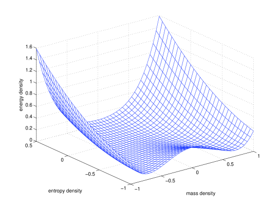
Figure 1: Internal energy density $\tilde{\varepsilon}_{0}(\tilde{\eta},\tilde{\rho})$ of a homogeneous fluid near critical point corresponding to $(\tilde{\eta}_{c},\tilde{\rho}_{c},\tilde{\varepsilon}_{c})=(0,0,0)$ when we chose $\tilde{\chi}=0.35$ .

4 Integration of equations in planar interfaces

We consider a planar interface and assume that all fields depend only on transverse space-variable $z$. We denote $\varphi^{\prime}$ the derivative of any field $\varphi$ with respect to $z$.

4.1 System of equilibrium equations

System of equilibrium equations (6) completed by the state law reads in term of new $\widetilde{\ }\,$- equivalent quantities,

$$\left\{\begin{array}[]{l}\tilde{C}_{0}\,(\tilde{\Lambda}\tilde{\rho}^{\prime})^{\prime}+\tilde{D}_{0}\,(\tilde{\Lambda}\tilde{\eta}^{\prime})^{\prime}+\tilde{F}_{0}\,(\tilde{\Lambda}\tilde{\varepsilon}^{\prime})^{\prime}=\tilde{\Lambda}\tilde{\mu}-\tilde{\mu}_{{}_{0}},\\ \tilde{D}_{0}\,(\tilde{\Lambda}\tilde{\rho}^{\prime})^{\prime}+\tilde{E}_{0}\,(\tilde{\Lambda}\tilde{\eta}^{\prime})^{\prime}+\tilde{G}_{0}\,(\tilde{\Lambda}\tilde{\varepsilon}^{\prime})^{\prime}=\tilde{\Lambda}\tilde{T}-\tilde{T}_{0},\\ \tilde{F}_{0}\,(\tilde{\Lambda}\tilde{\rho}^{\prime})^{\prime}+\tilde{G}_{0}\,(\tilde{\Lambda}\tilde{\eta}^{\prime})^{\prime}+\tilde{H}_{0}\,(\tilde{\Lambda}\tilde{\varepsilon}^{\prime})^{\prime}=1-\tilde{\Lambda},\\ \tilde{\cal L}_{0}(\tilde{\varepsilon},\tilde{\eta},\tilde{\rho})-\tilde{Q}(\tilde{\rho}^{\prime},\tilde{\eta}^{\prime},\tilde{\varepsilon}^{\prime})=0,\end{array}\right.$$ (15)

where $\tilde{Q}(\tilde{\rho}^{\prime},\tilde{\eta}^{\prime},\tilde{\varepsilon}^{\prime}):=\frac{1}{2}\big{(}\tilde{C}_{0}\,\tilde{\rho}^{\prime 2}+\tilde{E}_{0}\,\tilde{\eta}^{\prime 2}+\tilde{H}_{0}\,\tilde{\varepsilon}^{\prime 2}+2\tilde{D}_{0}\,\tilde{\eta}^{\prime}\tilde{\rho}^{\prime}+2\tilde{F}_{0}\,\tilde{\rho}^{\prime}\tilde{\varepsilon}^{\prime}+2\tilde{G}_{0}\,\tilde{\varepsilon}^{\prime}\tilde{\eta}^{\prime}\big{)}$.

Multiplying the three first equations respectively by $\tilde{\rho}^{\prime}$, $\tilde{\eta}^{\prime}$, $\tilde{\varepsilon}^{\prime}$, summing and using the fourth equation derived with respect to $z$, leads to

$$2\Big{(}\tilde{\Lambda}\,\tilde{Q}(\tilde{\rho}^{\prime},\tilde{\eta}^{\prime},\tilde{\varepsilon}^{\prime})\Big{)}^{\prime}=\tilde{\varepsilon}^{\prime}-\tilde{\mu}_{{}_{0}}\tilde{\rho}^{\prime}-\tilde{T}_{0}\tilde{\eta}^{\prime},$$

which gives the first energy integral

$$2\tilde{\Lambda}\,\tilde{Q}(\tilde{\rho}^{\prime},\tilde{\eta}^{\prime},\tilde{\varepsilon}^{\prime})=\tilde{\varepsilon}-\tilde{\mu}_{{}_{0}}\tilde{\rho}-\tilde{T}_{0}\tilde{\eta}+\tilde{P}_{0},$$ (16)

or equivalently, by using (4),

$$(2\tilde{\Lambda}-1)\,\tilde{\varepsilon}=2\tilde{\Lambda}\,\tilde{\varepsilon}_{0}-\tilde{\mu}_{{}_{0}}\tilde{\rho}-\tilde{T}_{0}\tilde{\eta}+\tilde{P}_{0},$$ (17)

where the constant $\tilde{P}_{0}$ has the dimension of a pressure.

In the bulk the fields become constant and the equilibrium equations lead to

$$\tilde{\Lambda}\tilde{\mu}-\tilde{\mu}_{{}_{0}}=0,\quad\tilde{\Lambda}\tilde{T}-\tilde{T}_{0}=0,\quad 1-\tilde{\Lambda}=0,\quad\tilde{\varepsilon}-\tilde{\mu}_{{}_{0}}\tilde{\rho}-\tilde{T}_{0}\tilde{\eta}+\tilde{P}_{0}=0.$$

Hence $\tilde{\Lambda}=1$ and $\tilde{\mu}_{{}_{0}}$, $\tilde{T}_{0}$, $\tilde{P}_{0}$ are respectively the common values of the chemical potential, temperature and pressure in both bulk phases and we recover the usual global equilibrium conditions for planar interfaces.

We denote by superscripts ⁺ and ^- the values of the fields in the two bulk phases. From (11), (12), (13) we deduce the equalities of thermodynamical quantities $\tilde{\mu}_{0},\tilde{T}_{0},\tilde{P}_{0}$ in the two bulks phases

$$2\tilde{\eta}^{+}\tilde{\rho}^{+}+4(\tilde{\rho}^{+})^{3} =2\tilde{\eta}^{-}\tilde{\rho}+4(\tilde{\rho}^{-})^{3}=\tilde{\mu}_{0}$$ (18)

$$2\tilde{\chi}\tilde{\eta}^{+}+(\tilde{\rho}^{+})^{2} =2\tilde{\chi}\tilde{\eta}^{-}+(\tilde{\rho}^{-})^{2}=\tilde{T}_{0}$$ (19)

$$\tilde{\chi}(\tilde{\eta}^{+})^{2}+2\tilde{\eta}^{+}(\tilde{\rho}^{+})^{2}+3(\tilde{\rho}^{+})^{4} =\tilde{\chi}(\tilde{\eta}^{-})^{2}+2\tilde{\eta}^{-}(\tilde{\rho}^{-})^{2}+3(\tilde{\rho}^{-})^{4}=\tilde{P}_{0}.$$ (20)

Using (19), equations (18) and (20) can be written

$$\tilde{T}_{0}\tilde{\rho}^{+}+(4\tilde{\chi}-1)(\tilde{\rho}^{+})^{3} =\tilde{T}_{0}\tilde{\rho}^{-}+(4\tilde{\chi}-1)(\tilde{\rho}^{-})^{3}=\tilde{\chi}\tilde{\mu}_{0},$$

$$2\tilde{T}_{0}(\tilde{\rho}^{+})^{2}+3(4\tilde{\chi}-1)(\tilde{\rho}^{+})^{4} =2\tilde{T}_{0}(\tilde{\rho}^{-})^{2}+3(4\tilde{\chi}-1)(\tilde{\rho}^{-})^{4}=4\tilde{\chi}\tilde{P}_{0}-\tilde{T}_{0}^{2},$$

which implies

$$\Big{(}\tilde{T}_{0}+(4\tilde{\chi}-1)\big{(}(\tilde{\rho}^{+})^{2}+\tilde{\rho}^{+}\tilde{\rho}^{-}+(\tilde{\rho}^{-})^{2}\big{)}\Big{)}\big{(}\tilde{\rho}^{+}-\tilde{\rho}^{-}\big{)}=0,$$

$$\Big{(}2\tilde{T}_{0}+3(4\tilde{\chi}-1)\big{(}(\tilde{\rho}^{+})^{2}+(\tilde{\rho}^{-})^{2}\big{)}\Big{)}\big{(}(\tilde{\rho}^{+})^{2}-(\tilde{\rho}^{-})^{2}\big{)}=0.$$

Considering an interface between two distinct phases, we have $\tilde{\rho}^{+}\not=\tilde{\rho}^{-}$, thus

$$\tilde{T}_{0}+(4\tilde{\chi}-1)\big{(}(\tilde{\rho}^{+})^{2}+\tilde{\rho}^{+}\tilde{\rho}^{-}+(\tilde{\rho}^{-})^{2}\big{)}=0,$$

$$\Big{(}2\tilde{T}_{0}+3(4\tilde{\chi}-1)\big{(}(\tilde{\rho}^{+})^{2}+(\tilde{\rho}^{-})^{2}\big{)}\Big{)}\big{(}\tilde{\rho}^{+}+\tilde{\rho}^{-}\big{)}=0.$$

Subtracting to the second equation the product of the first one by $2\big{(}\tilde{\rho}^{+}+\tilde{\rho}^{-}\big{)}$ the system becomes

$$(4\tilde{\chi}-1)\big{(}\tilde{\rho}^{+}-\tilde{\rho}^{-}\big{)}^{2}\big{(}\tilde{\rho}^{+}+\tilde{\rho}^{-}\big{)}=0$$

$$\tilde{T}_{0}+(4\tilde{\chi}-1)\big{(}(\tilde{\rho}^{+})^{2}+\tilde{\rho}^{+}\tilde{\rho}^{-}+(\tilde{\rho}^{-})^{2}\big{)}=0.$$

As expected this system admits no solution when $\tilde{T}_{0}>0$, or equivalently when the temperature in the phases is greater than the critical one. Let us set $\tilde{T}_{0}:=-(4\tilde{\chi}-1)\,\kappa^{2}$, i.e.

$$\kappa:=\sqrt{\frac{-\tilde{T}_{0}}{4\tilde{\chi}-1}}.$$ (21)

The small quantity $\kappa$ measures the distance from the critical point. Using again $\tilde{\rho}^{+}\not=\tilde{\rho}^{-}$ we find

$$\tilde{\rho}^{+}=\kappa\quad{\rm and}\quad\tilde{\rho}^{-}=-\kappa,$$ (22)

from which we directly deduce,

$$\tilde{\eta}^{+}=\tilde{\eta}^{-}=-2\,\kappa^{2},\quad\tilde{\mu}_{0}=0,\quad\tilde{\varepsilon}^{+}=\tilde{\varepsilon}^{-}=\tilde{P}_{0}=(4\chi-1)\kappa^{4}.$$ (23)

4.2 The rescaling process

In view of Eqs. (21), (22), (23) the values of $\tilde{\rho}$ and $\tilde{\eta}$ in the phases lead to the natural rescaling

$$\check{\rho}:=\kappa^{-1}\tilde{\rho},\quad\check{\eta}:=\kappa^{-2}\tilde{\eta},\quad\check{\varepsilon}:=\kappa^{-4}\tilde{\varepsilon},\quad\check{z}:=\kappa z$$ (24)

and system (15) becomes

$$\left\{\begin{array}[]{l}\tilde{C}_{0}\,(\tilde{\Lambda}\check{\rho}^{\prime})^{\prime}+\tilde{D}_{0}\,\kappa\,(\tilde{\Lambda}\,\check{\eta}^{\prime})^{\prime}+\tilde{F}_{0}\,\kappa^{3}\,(\tilde{\Lambda}\check{\varepsilon}^{\prime})^{\prime}=\tilde{\Lambda}\big{(}2\check{\eta}\check{\rho}+4\check{\rho}^{3}\big{)},\\ \tilde{D}_{0}\,\kappa\,(\tilde{\Lambda}\,\check{\rho}^{\prime})^{\prime}+\tilde{E}_{0}\,\kappa^{2}\,(\tilde{\Lambda}\check{\eta}^{\prime})^{\prime}+\tilde{G}_{0}\,\kappa^{4}\,(\tilde{\Lambda}\check{\varepsilon}^{\prime})^{\prime}=\tilde{\Lambda}\big{(}2\tilde{\chi}\check{\eta}+\check{\rho}^{2}\big{)}+(4\tilde{\chi}-1),\\ \tilde{F}_{0}\,\kappa^{3}\,(\tilde{\Lambda}\check{\rho}^{\prime})^{\prime}+\tilde{G}_{0}\,\kappa^{4}\,(\tilde{\Lambda}\check{\eta}^{\prime})^{\prime}+\tilde{H}_{0}\,\kappa^{6}\,(\tilde{\Lambda}\check{\varepsilon}^{\prime})^{\prime}=1-\tilde{\Lambda},\end{array}\right.$$ (25)

where the space derivatives are now relative to $\check{z}$. Hence $\tilde{\Lambda}=1+O(\kappa^{3})$ and at the first order with respect to the small parameter $\kappa$,

$$\left\{\begin{array}[]{l}\displaystyle\tilde{C}_{0}\,\check{\rho}^{\prime\prime}=2\check{\eta}\check{\rho}+4\check{\rho}^{3},\\ \displaystyle 0=2\tilde{\chi}\check{\eta}+\check{\rho}^{2}+(4\tilde{\chi}-1),\end{array}\right.$$ (26)

which gives by elimination of $\check{\eta}$,

$$\frac{\tilde{\chi}\tilde{C}_{0}}{(4\tilde{\chi}-1)}\,\check{\rho}^{\prime\prime}=\check{\rho}^{3}-\check{\rho}.$$ (27)

Multiplying by $\check{\rho}^{\prime}$, integrating and taking into account (22), we get

$$\frac{\tilde{\chi}\tilde{C}_{0}}{(4\tilde{\chi}-1)}\,\frac{\check{\rho}^{\prime 2}}{2}=\frac{1}{4}\left(\check{\rho}^{2}-1\right)^{2}.$$ (28)

Hence the mass density profile $\check{\rho}_{eq}$ at equilibrium across an interface has the classical representation (cf. [32] p. 251)

$$\check{\rho}_{eq}(\check{z})=\tanh(\frac{\check{z}}{\ell})$$ (29)

where

$$\ell=\sqrt{\frac{2\tilde{\chi}\check{C}_{0}}{(4\tilde{\chi}-1)}}.$$ (30)

Note that this well known profile is an exact solution of (27) but results from several approximations. It is valid only for a planar interface lying far from the boundaries of the domain. Moreover considering the polynomial form (11) for the energy is clearly an approximation as well as neglecting the terms of lower order in (18), (19) and (20).

Using (12) and (26) we obtain that the temperature through the interface is constant at the first order:

$$\check{T}_{eq}=2\tilde{\chi}\check{\eta}_{eq}+(\check{\rho}_{eq})^{2}=-(4\tilde{\chi}-1).$$

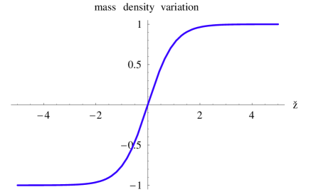
Figure 2: Classical density profile of the normalized density ( $\check{\rho}\in]-1,+1[$ ) associated with (29) and (30); the $x$-axis unit is $\ell$.

However the second equation of system (25) gives a more accurate information about the temperature profile through the interface; indeed, at order $\kappa$,

$$\tilde{D}_{0}\,\kappa\,\check{\rho}^{\prime\prime}=2\tilde{\chi}\check{\eta}+\check{\rho}^{2}+(4\tilde{\chi}-1)+O(\kappa^{2}).$$ (31)

That is

$$\check{T}_{eq} =-(4\tilde{\chi}-1)+\kappa\,\tilde{D}_{0}\,{\check{\rho}_{eq}^{\prime\prime}}+O(\kappa^{2})$$

$$=-(4\tilde{\chi}-1)+\kappa\,\frac{(4\tilde{\chi}-1)}{\tilde{\chi}}\,\frac{\tilde{D}_{0}}{\tilde{C}_{0}}\,\left[{\check{\rho}_{eq}^{3}}-{\check{\rho}_{eq}}\right]+O(\kappa^{2}).$$

Consequently,

$$\check{T}_{eq}=(4\tilde{\chi}-1)\Bigg{(}-1+\frac{\kappa}{\tilde{\chi}}\,\frac{\tilde{D}_{0}}{\tilde{C}_{0}}\left({\tanh^{3}\left(\frac{\check{z}}{\ell}\right)}-{\tanh\left(\frac{\check{z}}{\ell}\right)}\right)\Bigg{)}+O(\kappa^{2}).$$ (32)

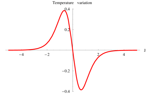
Figure 3: Variation of normalized temperature $\check{T}_{eq}+(4\chi-1)$ through the interface near the critical point. The $x$-axis unit is $\ell$ and the $y$-axis unit is $\displaystyle\kappa\,\frac{(4\tilde{\chi}-1)}{\tilde{\chi}}\,\frac{\tilde{D}_{0}}{\tilde{C}_{0}}$.

Note that in Eq.(32) the variation of the temperature across the interface is no more monotonic (see Fig. 3). Moreover, the variation of temperature $\check{T}_{eq}$ is multiplied by the small parameter $\kappa$ and is negligible with respect to the variation of $\check{\rho}_{eq}$.

5 Surface tension

Surface tension $\sigma$ of a plane liquid-vapor interface corresponds to the excess of free energy $\tilde{e}:=\tilde{\varepsilon}-\tilde{T}\tilde{\eta}$ inside the interface. Using (12) and (14), we have

$$\tilde{e}=\frac{4\tilde{\chi}-1}{4\tilde{\chi}}\big{(}\tilde{\rho}^{4}-2\tilde{\kappa}^{2}\tilde{\rho}^{2}-\kappa^{4}(4\tilde{\chi}-1)\big{)}+\tilde{Q}(\tilde{\rho}^{\prime},\tilde{\eta}^{\prime},\tilde{\varepsilon}^{\prime})$$

As, in the bulk, we have

$$\tilde{e}^{+}=\tilde{e}^{-}=-(4\tilde{\chi}-1)\kappa^{4},$$

surface tension is

$$\tilde{\sigma} :=\int_{-\infty}^{+\infty}\left(\tilde{e}+(4\tilde{\chi}-1)\kappa^{4}\right)dz=\int_{-\infty}^{+\infty}\left(\frac{4\tilde{\chi}-1}{4\tilde{\chi}}(\tilde{\rho}^{2}-\tilde{\kappa}^{2})^{2}+\tilde{Q}(\tilde{\rho}^{\prime},\tilde{\eta}^{\prime},\tilde{\varepsilon}^{\prime})\right)dz$$

$$=\kappa^{3}\int_{-\infty}^{+\infty}\left(\frac{4\tilde{\chi}-1}{4\tilde{\chi}}(\check{\rho}^{2}-1)^{2}+\tilde{Q}(\check{\rho}^{\prime},\kappa\check{\eta}^{\prime},\kappa^{3}\check{\varepsilon}^{\prime})\right)d\check{z}.$$ (33)

At the first order with respect to $\kappa$, we obtain

$$\tilde{\sigma} =\kappa^{3}\int_{-\infty}^{+\infty}\left(\frac{4\tilde{\chi}-1}{4\tilde{\chi}}(\check{\rho}^{2}-1)^{2}+\frac{1}{2}\tilde{C}_{0}\,\check{\rho}^{\prime 2}\right)d\check{z}+O(\kappa^{4})$$ (34)

$$=\kappa^{3}\int_{-1}^{+1}\left(\sqrt{\frac{(4\tilde{\chi}-1)\tilde{C}_{0}}{2\tilde{\chi}}}\,(1-\check{\rho}^{2})\right)d\check{\rho}+O(\kappa^{4})$$

$$=\kappa^{3}\,\frac{4}{3}\,\sqrt{\frac{(4\tilde{\chi}-1)\tilde{C}_{0}}{2\tilde{\chi}}}\,+O(\kappa^{4})$$ (35)

Thus, at the leading order, equilibrium values and surface tension are those given by the Cahn-Hilliard theory : the effect of the gradients of entropy and energy densities are negligible. A more accurate description could be obtained : terms of order $\kappa^{4}$ would come from (i) the perturbation of system (26) by taking into account the coupling term $\tilde{D}_{0}$ and (ii) the introduction of the same coupling term in (34).

6 Conclusion

We have obtained the mass density and temperature profiles through an interface near the critical point. Our results present some similarities with the ones obtained in [24] for fluid mixtures where two mass densities have the role played here by mass and entropy densities. The differences lie in the fact that we are not here impelled to deal with combinations of densities and also in the fact that the notion of critical point is more complex in the case of a mixture where non-monotonic profiles can be obtained at the leading order.

We have introduced a state law in which all gradients are considered with respect to mass, entropy and energy densities. At our knowledge, it is the first time that this though natural assumption is used. In this framework, we confirm the conjecture made by Rowlinson and Widom [32] that, near the critical point, the variations of temperature inside the interfacial layer are negligible. This result is mainly due to the fact that the variations of entropy density are negligible with respect to the variations of mass density.

Data accessibility statement. This work does not have any experimental data.

Competing interests statement. We have no competing interest.

Author’s contribution. H.G. and P.S. conceived the mathematical model, interpreted the results, and wrote together the paper.

Acknowledgements. P.S. thanks the Laboratoire de Mécanique et d’Acoustique (Marseille) for its hospitality.

Funding statement. This work was supported by C.N.R.S.

Ethics statement. This work is original, has not previously been published in any Journal and is not currently under consideration for publication elsewhere.

References

- [1] B. Widom, What do we know that van der Waals did not know?, Physica A, 263 (1999) 500–515.
- [2] H. Gouin, Energy of interaction between solid surfaces and liquids, The Journal of Physical Chemistry B, 102 (1998) 1212–1218 & arXiv:0801.4481.
- [3] J.D. van der Waals, The thermodynamic theory of capillarity under the hypothesis of continuous variation of density, translation by J.S. Rowlinson, Journal of Statistical Physics, 20 (1979) 200–244.
- [4] J. Korteweg, Sur la forme que prennent les équations du mouvement des fluides si l’on tient compte des forces capillaires, Archives Néerlandaises, 2, n6 (1901) 1–24.
- [5] S. Ono, S. Kondo, Molecular theory of surface tension in liquid in ”Structure of liquids”, S. Flügge (ed.) Encyclopedia of Physics, X, Springer, Berlin, 1960.
- [6] J.W. Cahn, J.E. Hilliard, Free energy of a nonuniform system, III. Nucleation in a two-component incompressible fluid, Journal of Chemical Physics, 31 (1959) 688–699.
- [7] P. Casal, La capillarité interne, Cahier du Groupe Français de Rhéologie. CNRS VI (1961) 31- 37.
- [8] P. Casal, H. Gouin, Connexion between the energy equation and the motion equation in Korteweg’s theory of capillarity, Comptes Rendus de l’Académie des Sciences de Paris II, 300 (1985) 231 -233.
- [9] F. dell’Isola, H. Gouin, P. Seppecher, Radius and surface tension of microscopic bubbles by second gradient theory, Comptes Rendus de l’Académie des Sciences de Paris IIb, 320 (1995) 211–216.
- [10] F. dell’Isola, H. Gouin, G. Rotoli, Nucleation of spherical shell-like interfaces by second gradient theory: numerical simulations, European Journal of Mechanics, B/Fluids, 15 (1996) 545–568.
- [11] P. Casal, La théorie du second gradient et la capillarité, Comptes Rendus de l’Académie des Sciences de Paris A 274, (1972) 1571 -1574.
- [12] P. Seppecher, Equilibrium of a Cahn and Hilliard fluid on a wall: influence of the wetting properties of the fluid upon stability of a thin liquid film, European Journal of Mechanics B/fluids, 12 (1993) 61–84.
- [13] P. Seppecher, Moving contact line in the Cahn-Hilliard theory, International Journal of Engineering Science, 34 (1995) 977–992.
- [14] H. Gouin, W. Kosiński, Boundary conditions for a capillary fluid in contact with a wall, Archives of Mechanics, 50 (1998) 907–916 & arXiv:0802.1995
- [15] H. Gouin, Liquid Nanofilms. A mechanical model for the disjoining pressure, International Journal of Engineering Science, 47 (2009) 691–699 & arXiv:0904.1809
- [16] H. Gouin, Statics and dynamics of fluids in nanotubes. Note di Matematica, 32 (2012) 105–124 & arXiv:1311.2303.
- [17] M. Gărăjeu, H. Gouin, G. Saccomandi, Scaling Navier-Stokes equation in nanotubes, Physics of fluids, 25 (2013) 082003 & arXiv:1311.2484
- [18] H. Gouin, S. Gavrilyuk, Dynamics of liquid nanofilms, International Journal of Engineering Science, 46 (2008) 1195–1202 & arXiv:0809.3489
- [19] H. Gouin, Solid-liquid interaction at nanoscale and its application in vegetal biology, Colloids and Surfaces A, 383 (2011) 17–22 & arXiv:1106.1275
- [20] H. Gouin, The watering of tall trees - Embolization and recovery, Journal of Theoretical Biology, 369 (2015) 42–50 & arXiv:1404.4343
- [21] P. Germain, The method of the virtual power in continuum mechanics - Part 2: microstructure, SIAM Journal of Applied Mathematics, 25 (1973) 556–575.
- [22] F. Dell Isola, P. Seppecher, A. Della Corte, The postulations à la d’Alembert and à la Cauchy for higher gradient continuum theories are equivalent: a review of existing results, Proceedings of the Royal Society A, 471 (2015) 20150415.
- [23] H. Gouin, T. Ruggeri, Mixtures of fluids involving entropy gradients and acceleration waves in interfacial layers, European Journal of Mechanics B/Fluids, 24 (2005) 596-613 & http://arXiv:0801.2096
- [24] H. Gouin, A. Muracchini, T. Ruggeri, Travelling waves near a critical point of a binary fluid mixture, International Journal of Non-Linear Mechanics, 47 (2012) 77–84 & http://arXiv:1110.5137
- [25] F. dell’Isola, K. Hutter, Continuum mechanical modelling of the dissipative processes in the sediment-water layer below glaciers, Comptes Rendus de l’Académie des Sciences de Paris IIb, 325 (1997) 449–456.
- [26] V.A. Eremeyev, F.D. Fischer, On the phase transitions in deformable solids, Zeitschrift für Angewandte Mathematik und Mechanik (ZAMM), 90 (2010) 535–536.
- [27] F. dell’Isola, P. Seppecher, A. Madeo, How contact interactions may depend on the shape of Cauchy cuts in N-th gradient continua: approach ”à la D’Alembert”, Zeitschrift für Angewandte Mathematik und Physik (ZAMP), 63 (2012) 1119–1141.
- [28] A. Bertram, S. Forest, The thermodynamics of gradient elastoplasticity, Continuum Mechanics and Thermodynamics, 26 (2014) 269–286.
- [29] Ornstein L.S., Statistical theory of capillarity, in: KNAW, Proceedings, 11, Amsterdam, (1909) 526-542.
- [30] H.C. Hamaker, The London-van der Waals attraction between spherical particles, Physica, 4 (1937) 1058–1072.
- [31] R. Evans, The nature of liquid-vapour interface and other topics in the statistical mechanics of non-uniform classical fluids, Advances in Physics, 28 (1979) 143–200.
- [32] J.S. Rowlinson, B. Widom, Molecular theory of capillarity, Clarendon Press, Oxford and Google books, 2012.
- [33] P. Casal, H. Gouin, Equation of motion of thermocapillary fluids, Comptes Rendus de l’Académie des Sciences de Paris II, 306 (1988) 99 -104.
- [34] H. Gouin, Properties of thermocapillary fluids and symmetrization of motion equations, International Journal of Non-Linear Mechanics, 85 (2016) 152–160.
- [35] S. Forest, M. Amestoy, Hypertemperature in thermoelastic solids, Comptes Rendus Mécanique, 336 (2008) 347–353.
- [36] S. Forest, E. C. Aifantis, Some links between recent gradient thermo-elasto-plasticity theories and the thermomechanics of generalized continua, International Journal of Solids and Structures, 47 (2010) 3367–3376.
- [37] M.H. Maitournam, Entropy and temperature gradients thermomechanics: Dissipation, heat conduction inequality and heat equation, Comptes Rendus Mécanique, 340 (2012) 434–443.
- [38] C. Domb, The critical point, Taylor and Francis, London, 1996.