Meta-learning for feature selection

Abstract

A general formulation of optimization problems in which various candidate solutions may use different feature-sets is presented, encompassing supervised classification, automated program learning and other cases. A novel characterization of the concept of a “good quality feature” for such an optimization problem is provided; and a proposal regarding the integration of quality based feature selection into metalearning is suggested, wherein the quality of a feature for a problem is estimated using knowledge about related features in the context of related problems. Results are presented regarding extensive testing of this ”feature metalearning” approach on supervised text classification problems; it is demonstrated that, in this context, feature metalearning can provide significant and sometimes dramatic speedup over standard feature selection heuristics.

1 Introduction

The critical importance of feature selection in classification and other optimization tasks is well understood by all real-world practitioners of these technologies, yet is relatively under-addressed in the theoretical literature. Some rigorous characterizations of feature quality in terms of concepts like mutual information and separability have been articulated (see [Bla09], [DWBB09], [KDBB10] for reviews) but these do not yet constitute a comprehensive theory of feature quality.

Here we present a novel theory of feature quality in a very general setting. We begin by describing a general class of optimization problems in which various candidate solutions may use different feature-sets. This class encompasses supervised classification, automated program learning and other cases. We then present a formal characterization of what constitutes a “good quality feature” or a “good quality feature subset” for such an optimization problem. While new in many respects, the core ideas come from previous practical work in feature quality estimation in the context of supervised classification of microarray and SNP data [GSMP08].

Finally we discuss the application of these ideas to metalearning [BCSV08]. Our definition of feature quality could be used straightforwardly to drive feature selection, but the issue that arises here is that a fairly large knowledge base of potential problem solutions may be needed in order to get a reliable estimate of feature quality. We suggest that metalearning may provide a way around this issue in many cases, via allowing knowledge about the impact of features on solution quality to be transferred from one problem to other related problems. That is, the quality of a feature for a problem may be estimated using knowledge about related features in the context of related problems. In some contexts, this may be a more important variety of metalearning than the more common application of metalearning to algorithm selection or parameter tuning. Sometimes feature selection may actually be the hard part of a machine learning problem, and the place where the assistance of metalearning is most badly needed.

1.1 Evaluation of Feature Metalearning for Text Classification

The bulk of the paper describes some computational experiments carried out in order to provide an initial exploration of the proposed approach to feature metalearning. These experiments show that feature metalearning has significant capability to speed up text classification performance.

In these experiments, we created a database called the MetaDB, which stores learning problems together with the data-features found most useful for solving them; and then to use the information in the MetaDB to initialize the feature selection process for new problems, thus accelerating the feature selection process for these new problems. This is a very general concept; here we explore it in the specific context of binary text classification, but we believe the concept deserves to be explored much more broadly.

Specifically, in the experiments reported here, we have applied feature metalearning to techtc300 text classification dataset collection [Gab04, DGM04], as well as similar collections generated using software we developed specially for this experiment [Gei11]. The datasets in this collection are all built upon the DMOZ database [Net] that classifies a large number of websites according to a certain ontology. Each dataset contains texts of websites that belong to a certain category vs texts of websites belonging to another category. An example dataset in the collection would be:

• 278 documents (i.e. websites) belonging to the positive category

  $$Top/Arts/Music/Instruments/$$

• 257 documents belonging to the negative category

  $$Top/Health/Medicine/Education$$

The techtc300 collection contains 300 different datasets of this nature.

In the experiments we report here, each such dataset is pre-processed and transformed into feature vectors where each feature marks the presence or absence of a word in its corresponding document, and the target associated with each feature vector indicates whether the document belongs to the positive category or not. This is a simplistic approach to assigning feature vectors to texts, but proved adequate for initial exploration of the feature metalearning concept.

Crawling the DMOZ database allows one to generate very large collections of datasets. However the datasets within a given collection can be rather distant semantically, which increases the difficulty of enabling effective feature metalearning learning. However, we managed nevertheless to achieve positive feature metalearning results.

Specifically, we have shown that, in the text classification context at least,

• If the collection of datasets is sufficiently ”dense”, in the sense that a dataset generally has some fairly close neighbors in dataset-space, then feature metalearning gives positive speedup (over a more straightforward, non metalearning based feature selection process) and doesn’t degrade the quality of the final answer

• The speedup is greatest in the case where one needs a quick answer and doesn’t allocate enough time to the problem-solving process to find an optimal feature set, but only needs a ”best I can find in the time available” feature set

At the end of the report we will present some of our ideas for how to surmount or weaken these limitations, which we did not have time to explore yet.

We believe the feature metalearning approach has great promise to dramatically accelerate machine learning in cases where there is a large number of relatively similar problems with features drawn from a common feature space. The initial algorithms reported here have sufficed to demonstrate the viability of the approach, and explore some of its properties. Refining them via future research should ultimately lead to the development of extremely powerful feature metalearning systems.

2 A Formal Characterization of Feature Quality

2.1 A General Class of Optimization Problems

We begin by articulating a fairly general class of optimization problems to which the problems of “feature selection” and “feature quality” pertain.

Suppose we have a maximization problem with objective function $\phi:G\rightarrow W$, where $W$ is a positive bounded subset of the real line, and $G$ is a space of functions so that for some fixed sets $B$ and $\theta=\prod_{i\in I}\theta_{i}$ (the Cartesian product of all “variables” or “features”), each $g\in G$ has the form: $g:A\rightarrow B$ for some $A=A_{g}=\prod_{i\in J}\theta_{i},J\subseteq I$.

For instance, one may have $B$ = the real line, and $\theta$ = 100-dimensional real space. Then, each $g\in G$ would map some n-dimensional space for $n\leq 100$ into some bounded subset of the real line. The maximization problem then involves finding some $g$ of this nature, that maximizes some criterion.

Or more interestingly, one may have a traditional categorization problem, in which case $B$ is a set of category labels, and each $g$ is a “classification model” assigning a list of feature values to a category. In this case the objective function $\phi$ calculates the F-measure or some other measure of the quality of the classification model.

Or one may have an automated program learning problem, in which the $g$ are programs mapping sets of input variables into outputs lying in $B$.

In any of these situations, one pertinent question is: which “features” $\theta_{i}$ are most useful for solving the maximization problem? And which feature-sets are most valuable? This is an algorithmic question (how to find the useful features) but also a conceptual question (how to define what it means for a feature to be useful).

2.2 Formalizing Feature Quality

Next, in order to define the quality of an individual feature $\theta_{i}$ with respect to an objective function $\phi$, we will assume that we have some measure $q(\theta_{i},g)$ of the quality of a feature $\theta_{i}$ with respect to a particular function $g\in G$. We would like $q(\theta_{i},g)\in[0,1]$, where for instance

• if the variable $\theta_{i}$ is not used at all in $g$ then $q(\theta_{i},g)=0$

• if changing the value of $\theta_{i}$ changes the output value of $g$ (at least sometimes), then $q(\theta_{i},g)>0$

Our definition of feature quality for $\phi$ can be used with many different approaches to $q$; but a little later we will describe one particular approach to $q$ that seems potentially promising.

Given the above, we define the quality of feature $\theta_{i}$ with respect to objective function $\phi$ as

$$Q(\theta_{i},\phi)=\int q(\theta_{i},g)T(\phi(g))d\mu(g)$$

where $\mu(g)$ represents a prior distribution over the $g$ functions, e.g. perhaps a simplicity-based prior such as the Solomonoff prior. $T$ represents a fitness distortion.

This tells, basically, the average degree to which variation in the feature $\theta_{i}$ affects the output of the functions $g$, with a weighting in the average to value $g$ that are close to optimizing $\phi$. It is a generalization of the definition of “feature importance” used in the OpenBiomind toolkit http://code.google.com/p/openbiomind/, used to good effect in a number of practical genomics classification problems, and described in [GSMP08].

We may start with $T(w)=\left(\frac{\phi(g)}{sup_{g}\phi(g)}\right)^{p}$, that is the fitness distortion normalizes the fitness and emphasizes good fits. The exponent $p$ weights how much the near-optimality of $g$ figures into the calculation. Of course other distortion functions besides the $p$-power could be used, here, but for the moment the $p$-power seems to give adequate flexibility.

At first glance it may seem that this feature quality measure looks at each variable in isolation, but actually it considers interactions, because the functions $g$ combine the variables in various ways.

The next question is how to consider multiple variables jointly, e.g. how to think about the combined utility of two features $\theta_{i}$ and $\theta_{j}$ (or sets of three or more features). The simplest approach is just to consider a set $S$ of features as if it were a single feature, and apply the above definition directly to this single amalgamated feature, i.e.

$$Q(S,\phi)=\int q(S,g)T(\phi(g))d\mu(g)$$

where $S$ is a set of more than one $\theta_{j}$. This works perfectly well so long as one has a definition of $q(S,g)$.

Finally, note that if $T(\phi(g))$ is defined as the probability of function $g$ meeting some objective $o$, then $Q(S,\phi)$ is the expectation of the quality of $S$ (as defined by $q$) relative to the given optimization problem.

2.3 Feature Quality Relative to a Specific Function $g$

One potentially interesting way to define $q$ is using the Fisher information. To apply the Fisher information here, first we will translate the function $g$ being optimized into a probability density function. So we can consider the output value of $g$ as a random variable $X_{g}$, and the density $f_{g}(X_{g})$ is then defined by the standard equation $P(X_{g}\in D)=\int_{x\in D}df_{g}(x)$.

At each particular $\theta$ vector, we may then define the Fisher information $\mathcal{I}_{g}(\theta)_{i}$ corresponding to the variable $\theta_{i}$. This tells, roughly speaking, how much the output of $g$ varies, as one varies $\theta_{i}$ in the neighborhood of $\theta$. We may then define

$$q(\theta_{i},g)=\frac{\int\mathcal{I}_{g}(\theta)_{i}d\nu(\theta)}{max_{j}\int\mathcal{I}_{g}(\theta)_{j}d\nu(\theta)}$$

where $\nu$ is a prior distribution over $\theta$ values.

The same definition works for a feature-set S, i.e.

$$q(S,g)=\frac{\int\mathcal{I}_{g}(\theta)_{S}d\nu(\theta)}{max_{S^{\prime}}\int\mathcal{I}_{g}(\theta)_{S^{\prime}}d\nu(\theta)}$$

(where $S^{\prime}$ is assumed to be a feature-set drawn from $\theta$ with the same cardinality as $S$), the only complication here being that one must define $\mathcal{I}_{g}(\theta)_{S}$ more subtly, e.g. as the average Fisher information $\mathcal{I}_{g}(\theta)$ calculated along all geodesic paths from $\theta$ to other vectors $\theta^{\prime}$ obtainable via varying only features in S.

3 Methodology

In this section we explain in detail the steps of the methodology employed in our experiments in feature metalearning for text classification.

3.1 Overview of the Meta-algorithm

Given a new problem D (i.e. a classification task taken from some techtcX collection, where X typically represents the size of the collection), the chain of tasks follows:

1. Get initial features from the MetaDB (explained below), supposedly belonging to the set of best features of D, by selecting the best features of problems nearby D (see Section 3.3).

2. Run a feature-search method for feature selection using the set of features obtained in the previous step to initialize the search and hopefully speed it up (see Section 3.4).

3. Run the learning task with the set of features selected in the previous step (see Section 3.5).

4. Given the information obtained in the previous step, update the MetaDB; that is, associate the problem with its best features plus other useful information such as their quality (see Section 3.6).

5. Wait for a new problem and go back to step 1.

3.2 MetaDB

The MetaDB is a repository associating problems already explored to features found to be useful to that problem. Technically speaking it is an XML file containing for each problem

1. A unique ID of the problem (here, the path of its corresponding dataset).

2. The set of features with their feature qualities, $q$ and $Q$ as defined in Sections 3.4.2 and 3.6 respectively.

3. Information such as the minimum and maximum score obtainable for that dataset to normalize the fitness function of the learning problem.

4. The set of candidates with their scores obtained during learning.

Additionally all problems already explored are stored in a covertree [BKL06] for fast retrieval.

3.3 Feature Transfer

In absence of metalearning the search starts from the empty set. With feature transfer the search starts from the feature set given during the step 1 of the meta-algorithm described in Section 3.1.

Positive (resp. negative) transfer is said to have occurred if the search is faster (resp. slower) when starting from that given feature set rather than from the empty set, with similar feature quality obtained in both cases.

3.3.1 Formula to select features to transfer

Seeding the feature search for a new problem via selecting the entire feature set of nearby problems, hasn’t proved effective. This strategy might work if the problems involved was composed of very similar problems (for instance if all datasets were restricted to sentiment analysis of similar types of text). But in the situation we explored in our experiments, each dataset corresponds to a rather different classifier, sometimes pretty distant from each other semantically, such as Music vs Health, Business vs Movie, etc. So instead we chose to consider each feature of a new problem separately and decide based on appropriate heuristics whether it may be a good feature for the new problem or not.

The heuristics utilized may be interpreted as means of approximation

$$P_{D}(s)={\it probability\ that\ feature\ s\ is\ in\ the\ best\ feature\ set\ of\ D}$$

where $D$ is the dataset corresponding to the new problem instance. Then given a transfer threshold $t$ one selects all features $s$ belonging to the best feature sets of the k-nearest datasets so that $P_{D}(s)\geq t$. By setting the value $t$ adequately we hope to filter feature transfer so that positive ones occur significantly more often than negative ones.

3.3.2 Our heuristic

Estimating $P_{D}$ is not trivial, and in our work so far we have utilized a simple heuristic (which no doubt could be improved substantially):

$$P_{D}(s)=\frac{\sum_{i=1}^{k}w(d(D,D_{i}))\times Q(s,D_{i})}{\sum_{i=1}^{k}w(d(D,D_{i}))}$$

where

• $D_{1}$, …, $D_{k}$ are the k-nearest neighbors (according to the Jensen-Shannon divergence, briefly explained in Section 3.3.3),

• $d(D,D_{i})$ is the square root of the Jensen-Shannon divergence,

• $w(d)=1/(c+d^{2})$, where $c$ is a positive constant (arbitrarily fixed to 0.001 in our experiments),

• $Q(s,D_{i})$ is the quality of feature $s$ of the problem corresponding to dataset $D_{i}$.

The formula expresses that: if a feature is important w.r.t. nearby datasets of $D$, then it is likely to be important w.r.t. $D$, and this likelihood increases with the importance of the feature and the closeness of the neighbors. The definition of $w(d)$ is somewhat ad hoc, though functional, and will likely be refined via further experimentation.

3.3.3 Problem Distance: Jensen-Shannon Divergence

In our practical work so far, we have used the square root of the Jensen-Shannon divergence to measure distance between datasets. We made this choice because of its simplicity and manageability – it is always within $[0,1]$, and it is a true metric, which is important so that fast KNN query algorithms such as covertree can be used.

The Jensen-Shannon divergence (JSD for short) is defined as

$$\textit{JSD}(P,Q)=\frac{1}{2}\textit{KLD}(P,M)+\frac{1}{2}\textit{KLD}(Q,M)$$

where KLD is the Kullback-Leibler divergence and $M=\frac{1}{2}(P+Q)$.

The following examples illustrate how this measure is used here. Let’s assume the following dataset $D_{1}$

$$\begin{array}[]{|c|c|c|}\hline\cr word1&word2&target\\ \hline\cr 0&0&1\\ 0&1&1\\ 0&0&1\\ 1&0&0\\ \hline\cr\end{array}$$

where target represents whether the document of a certain row belongs to the positive ODP category corresponding to that dataset. Similarly $D_{2}$

$$\begin{array}[]{|c|c|c|}\hline\cr word1&word2&target\\ \hline\cr 1&1&1\\ 1&1&1\\ 1&0&1\\ 0&0&0\\ \hline\cr\end{array}$$

Let’s compute the square root of the JSD between $D_{1}$ and $D_{2}$. We must first represent the datasets as distributions, let’s start with $D_{1}$:

$$P_{D_{1}}(\{target\})=2/4=0.5$$

$$P_{D_{1}}(\{word2,target\})=1/4=0.25$$

$$P_{D_{1}}(\{word1\})=1/4=0.25$$

then $D_{2}$:

$$P_{D_{2}}(\{word1,word2,target\})=2/4=0.5$$

$$P_{D_{2}}(\{word1,target\})=1/4=0.25$$

$$P_{D_{2}}(\emptyset)=1/4=0.25$$

In this example $P_{D_{1}}$ and $P_{D_{2}}$ are entirely disjoint; as a result

$$d(D_{1},D_{2})=1$$

Let’s consider the dataset $D_{3}$

$$\begin{array}[]{|c|c|c|}\hline\cr word1&word2&target\\ \hline\cr 1&1&1\\ 0&1&1\\ 1&0&1\\ 0&0&0\\ \hline\cr\end{array}$$

with distributions

$$P_{D_{3}}(\{word1,word2,target\})=1/4=0.25$$

$$P_{D_{3}}(\{word2,target\})=1/4=0.25$$

$$P_{D_{3}}(\{word1,target\})=1/4=0.25$$

$$P_{D_{3}}(\emptyset)=1/4=0.25$$

Some intersection exists between $P_{D_{2}}$ and $P_{D_{3}}$ and the result of the square root of their JSD is

$$d(D_{2},D_{3})=0.3945$$

As shown in Section 4, in our case the distance is often 1 and rarely goes below 0.9. That is because the datasets generated by the techtc methodology contain many, many features, exceeding several dozens of thousands across all datasets. The heuristic we are using has been tuned in a way that accounts for this, and positive transfer occurs nevertheless. However this poses a problem for the k-nearest neighbor search as the dataset-space has a very large intrinsic dimensionality. In our experiments, even when using the largest collection, covertree based search would yield similar performance to naive search. There are certainly workarounds for this phenomenon, but we did not have time to implement and evaluate them in our work so far. For instance, one could compute the JSD only over a projection of generally important features, thus reducing the dimensionality of the space.

3.4 Feature Selection

To select a good feature set we search the space of feature sets that maximize a certain fitness function.

3.4.1 Algorithm to search features sets

The algorithm used to search the space of feature sets is a stochastic variation of hillclimbing. Let $S$ be a set of features. Let $d$ be the number of features to add or remove at once from $S$. Let $m$ be the maximum number of evaluations.

1. Start with $S=\emptyset$, $d=1$ and $m=M$ (where $M$ is given by the user).

2. Randomly add and/or remove $d$ features from $S$, to generate feature sets $S_{1}$ to $S_{h}$ (so each $S_{i}$ is at edit distance $d$ from $S$), where

   $$h=\min\left(\frac{m}{10},|F|^{d}\right)$$

   and $|F|$ is the total number of features in the dataset.

3. Set $m=m-h$.

4. Evaluate $S_{1}$ to $S_{h}$ (according to the fitness function defined below).

5. If there exists $S_{i}$ better than $S$, set $S=S_{i}$ and $d=1$. Otherwise increment $d$.

6. Go to step 2 unless $d=D$ or $m=0$.

Here $D$ is fixed to 5.

3.4.2 Fitness function to evaluate feature sets

We want feature sets which are informative but also as small as possible for two reasons

1. The smaller the feature set, the faster the learning algorithm.

2. The larger the feature set the less accurate is its measure of information gain.

With this in mind, the fitness function of a feature set is defined as

$$q(S)={\it MI}(S)^{2-r}\times c(S)^{r}$$

where ${\it MI}(S)=H(S;Y)$ is the mutual information of $S$ and the output $Y$, and $c(S)$ is a function that measures the confidence of ${\it MI}(S)$. The parameter $r$ measures how important confidence must be accounted for, the higher $r$ the more important the confidence, the smaller the best feature set will be found.

By using such a fitness function we not only aim at informational feature sets but also confident ones – which should also minimize overfitting during the learning process.

3.4.3 Feature set size and confidence

Inspired by OpenCog’s Probabilistic Logic Networks [GIGH08], we could define $c(S)$ as the probability that ${\it MI}(S)$ will be within a certain interval $[L,U]$ after k more observations.

But those methods are rather costly and complex to implement so we started with the following heuristic

$$c(S)=N/(N+b\times n)$$

where $n$ is the size of $S$ (i.e. the number of features) and $b$ is a parameter. More sophisticated and theoretically grounded heuristics are possible and we have done some work in this direction, but not implemented yet. That heuristic reflects the simple idea that the larger the number of features the less confidence the estimation of ${\it MI}(S)$ will be.

Using this heuristic formula, if $b$ tends to 0, $c(S)$ tends to 1; for that reason we have considered the parameter $b$ instead of the parameters $r$ defined in Section 3.4.2 to modulate the importance of the confidence (that way we only have one parameter to tweak).

3.5 Learning Task

Once a set of features has been selected the dataset is filtered and used as input of a classifier learner, here MOSES [Loo06], [Loo07], a probabilistic evolutionary program learning algorithm that we have used in many practical applications. The scores output by MOSES correspond to

minus the number of classification errors

as reported in Figures 3, 9, 13 and 18.

3.6 Update MetaDB

The results output by MOSES are then used to update the MetaDB with the feature quality measures. In Section 2 the notion of feature quality $Q$ is defined according to a fitness function to keep the definition as general as possible. In these specific experiments with text classification, however, we work on a specific class of fitness functions representing the error rate of a program fitting a dataset $D$. In this context it is essentially equivalent to just use $q(s)$ as defined in Section 3.4.2. That is what we have done in these experiments but it would certainly be interesting to try with $Q$ as well.

4 Experiments

We have conducted several experiments on techtcX collections to test the validity of those ideas.

4.1 Method

There are several ways to measure knowledge transfer, here we have focused mainly on the speed to select features. For that purpose each experiment are composed of the following steps

1. Run feature selection and learning over the entire dataset collection without any meta-learning taking place.

2. Mine the logs of the results obtained in the previous step and generate a list of accuracy targets, containing the maximum score obtained by feature selection for each problem in the sequence.

3. Run feature selection and learning over the entire dataset collection according to the meta-learning algorithm in Section 3.1, with the particularity that each feature selection process runs until it reaches its corresponding accuracy target defined in the previous step.

In both cases (with or without metalearning) the feature selection stops when a certain number of evaluations is reached.

Then we analyze the results and measure transfer learning in terms of acceleration of feature selection during the metalearning phase (step 3) as compared to the non-metalearning phase (step 1).

4.2 Parameters

The list of parameters we varied between our text classifications experiments is as follows:

• TCSize: the size of the techtc collection. Here the possible sizes are 300, 500. The techtc300 was directly taken from [Gab04]. The techtc500 was generated by our software [Gei11].

• PUber, NUber: the positive and negative uber categories where the subcategories are extracted to generate the datasets of the techtc collection. The techtc300 collection use both Top as uber category. The techtc500 uses Top/Arts/Music as uber positive category and Top/Science/Math as uber negative category.

• MI: the threshold of the mutual information used to pre-filter the techtc collection. The web is a rather messy place and it is not unusual to get dozens of thousands of features for a given dataset, lot of them being gibberish. For that reason we remove all features under a certain mutual information threshold. The higher the threshold the easier the feature selection task but with an additional risk of missing good features.

• FE: the number of evaluations allocated to feature selection (each evaluation measure how a feature set fits according to the fitness function defined in Section 3.4.2)

• t: the transfer threshold

Some other parameters have been left fixed

• The number of neighbors considered, $k=5$ in all experiments. We determined this number by conducting a few experiments which seemed to indicate that the number 5 works well.

• The number of evaluations used during the learning tasks was also fixed to 10000.

• The importance of the confidence in the feature selection fitness function (parameter $b$ defined in Section 3.4.3) was fixed to $b=5$. This setting limits the number of features selected to around a dozen in average, thus speeding up the experiments.

4.3 Results

We have conducted hundreds of experiments, using the techtc300 and the techtc500 collections. Following is a summary of some of the more interesting results.

Most figures represent the speed-up with and without meta-learning as a function of the iteration index of the sub-experiment in the series. We expect that if significant meta-level learning occurs, the speed-up will progressively increase as more problems have been solved and their quality features recorded for future use. Specifically the speed-up is defined as

$$\text{Speed-up}=\frac{num\ evals\ without\ metalearning}{num\ evals\ with\ metalearning}$$

We also report the arithmetic and geometric means of the speed-up, the former is intuitively clear, but the latter is a better measure of the overall speed-up.

4.4 Experiments with the techtc300, using Top categories

We present a series of experiments with the techtc300 collection, about 300 classification problems generated from the top categories, therefore possibly quite semantically distant.

4.4.1 Low feature selection effort, low transfer threshold

In this experiment, $MI=0.001$, $FE=1000$, $t=0.09$. Figure 1 represents for each feature selection task the speed-up (positive transfer) provided during metalearning as compared without metalearning.

The arithmetic mean of the speedup is 3.44, while the geometric mean is 1.05. The transfer threshold, 0.09, is quite low yet still yields some positive transfer. The reason behind that, besides the fact that the formula defined in Section 3.3.2 is a heuristic rather than the real probability, is that it does not account for the low number of evaluations ($FE=1000$) used to reach the accuracy target during the non-metalearning phase, as a consequence the accuracy targets are rather low (as shown in Figure 2) and therefore many more features can potentially speed-up the search.

Finally, me can check that the speed-up is not at the expense of the accuracy of the feature selection and the learning processes) as shown in Figures 2 and 3.

Figure 1: Speed-up for techtc300, $MI=0.001$, $FE=1000$, $t=0.09$

Figure 2: Feature selection scores for techtc300, $MI=0.001$, $FE=1000$, $t=0.09$

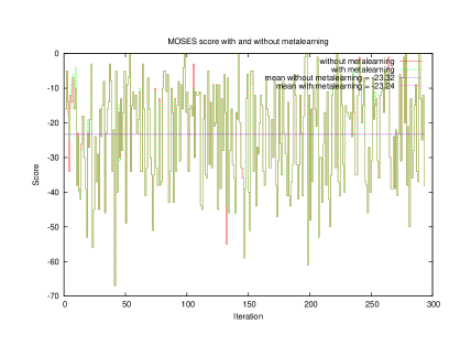
Figure 3: Learning scores for techtc300, $MI=0.001$, $FE=1000$, $t=0.09$

4.4.2 High feature selection effort, low transfer threshold

In this experiment we multiplied the feature selection effort by 10, $FE=10000$, while maintaining the same transfer threshold, $t=0.09$. As shown in Figure 4, except for iteration 61, that led to a massive speed-up, positive and negative transfers occurred roughly equally often. After inspecting the log we could explain the massive speed-up at iteration 61 by the fact that feature selection without metalearning selected, after 2710 evaluations, {submarin, uss, repeat} as best feature set, a rather small set with a high score of 0.89. But during metalearning our heuristic selected an even better feature set {navi, radio, uss} with a score of 0.9. As a result there was only one evaluation during the feature selection with metalearning as the accuracy target was immediately reached, yielding the massive speed-up of 2710. This speed-up raises the arithmetic mean up to 10.24, significantly higher than the one shown in Figure 1 but the geometric mean is actually slightly lower (1.04 instead of 1.05); as iteration 61 was an isolated case it does not contribute enough to yield better overall performance.

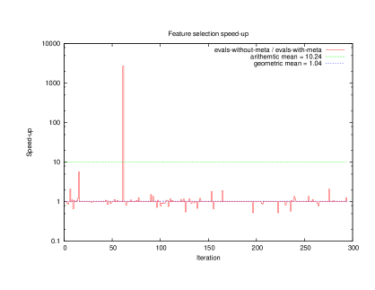
Figure 4: Speed-up for techtc300, $MI=0.001$, $FE=10000$, $t=0.09$

Figure 5 shows the number of features selected without and with metalearning as well as the number of feature transferred during metalearning and the number of feature in common with the transferred features and the selected feature during metalearning.

Figure 5: Number of features for techtc300, $MI=0.001$, $FE=10000$, $t=0.09$

4.4.3 High feature selection effort, very low transfer threshold

Decreasing the transfer threshold down to $t=0.01$ greatly increases the number of transfers (see Figure 6); however, as above, except a happy accident raising the arithmetic speed-up to 4.4 in one case, the geometric mean is actually below 1, which means that the overall performances have actually decreased during metalearning. This shows the importance of setting the transfer threshold high enough.

Figure 6: Speed-up for techtc300, $MI=0.001$, $FE=10000$, $t=0.01$

4.4.4 High feature selection effort, very high transfer threshold

As shown in Figure 7, increasing the transfer threshold up to $t=0.2$ eliminates most transfer including the 2 very good ones shown in Figures 4 and 6.

Figure 7: Speed-up for techtc300, $MI=0.001$, $FE=10000$, $t=0.2$

So as shown by this experiment and the previous one, increasing the number of evaluations up to 10000 for the techtc300 does not allow us to get any significant overall performance during metalearning. However using 10000 evaluations instead of 1000 yields significantly better scores with respect to feature selection as shown in Figure 8 (0.7 instead of 0.6 in Figure 2) and learning as shown in Figure 9 (-16.4 instead of -23.3 in Figure 3). So transfer learning in the case of the techtc300, although shown to happen and validate the idea, is not really beneficial in practice. Add to that, if the overall speed-up was more significant we would still need to take into account the additional computational cost of transferring features – which consists mostly, as we will see in the next experiments, of the calculations of the Jensen-Shannon divergences to find the nearest datasets.

Figure 8: Feature selection scores for techtc300, $MI=0.001$, $FE=10000$, $t=0.2$

Figure 9: Learning scores for techtc300, $MI=0.001$, $FE=10000$, $t=0.2$

4.5 Experiments with the techtc500, using Top categories Top/Arts/Music, Top/Science/Math

That next series of experiments was done using the techtc500, generated by us using [Gei11]. The results obtained below are not directly comparable with the ones obtained with the techtc300 collection because

1. They have been generated with different software that probably crawl the web differently and filter the information differently.

2. The top-level categories for the techtc500 are much narrower (Top/Arts/Music for positive and Top/Science/Math for negative) than the ones of the techtc300 (Top for both positive and negative).

3. The number of samples for each dataset is higher than with the techtc300 (about 200 on average for the techtc300, and about 300 on average for the techtc500).

4.6 Low feature selection effort, high transfer threshold

Here the pre-filtering threshold of the datasets is more aggressive ($MI=0.05$ instead of $MI=0.001$ as previously), mainly to decrease the computational time of the experiments (so each experiment still takes less than a day).

The number of evaluation for feature selection is rather low, $FE=1000$. And the transfer threshold moderately high, $t=0.1$. As shown in Figure 10, the results are quite encouraging, with a speed-up arithmetic mean of 27.17 and a geometric mean of 1.99. Moreover there is a clear indication that the frequency of massive speed-ups (occurring when the feature transfer find a better feature set right away) increases. This is obviously due to the fact that as measure as the experiment progresses the probability to find nearby datasets increases, as corroborated by Figure 11.

Figure 10: Speed-up for techtc500, $MI=0.05$, $FE=1000$, $t=0.1$

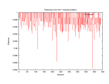
Figure 11: Distance to nearest neighbors for techtc500, $MI=0.05$, $FE=1000$, $t=0.1$

See Figures 12 and 13; one can check that the average feature selection and learning scores are similar with and without metalearning.

Figure 12: Feature selection scores for techtc500, $MI=0.05$, $FE=1000$, $t=0.1$

Figure 13: Learning scores for techtc500, $MI=0.05$, $FE=1000$, $t=0.1$

As it might be expected there is a correlation between the number of features transferred and speed-up; Figure 14 shows a Pearson correlation of 0.14, not high but substantial.

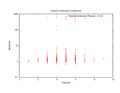
Figure 14: Feature transferred vs Speed-up for techtc500, $MI=0.05$, $FE=1000$, $t=0.1$

One may wonder what portion of this correlation is attributable to the distance. However Figure 15 shows a quite low Pearson correlation of 0.02 between the inverse of distance and speed-up. This low correlation is explained by the fact that the quality of the feature to be transferred plays an important role in the heuristic used for feature transfer.

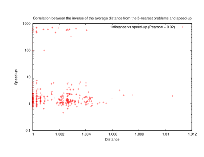
Figure 15: Inverse of distance vs Speed-up for techtc500, $MI=0.05$, $FE=1000$, $t=0.1$

Overall, in the experiments reported just above, we have observed some impressive speed-up for the techtc500 due to the greater number of datasets in the collection; and also more importantly, due to the higher similarity between these datasets, as all web pages constituting the datasets were drawn from the categories /Top/Arts/Music and /Top/Science/Math. However the number of evaluations for feature selection was still rather low in these experiments. Let see now how it goes when that number is 10000 instead of 1000.

4.7 High feature selection effort, very high transfer threshold

This experiment sets the number of evaluation for feature selection to $FE=10000$ which leads to higher feature selection and learning scores (as shown in Figures 17 and 18). We did try with 100000 but the improvement (in term of feature selection and learning scores) was not really substantial so this setting is “the real deal”. Due the highest quality target we need to increase the transfer threshold to $t=0.2$ to measure positive transfer learning.

As Figure 16 shows, although we do not get any massive speed-ups as in the previous experiment, the speed-up geometric mean, 1.22, is significant and the figure shows again a clear tendency toward faster feature selection as measure as the experiment progresses.

Figure 16: Speed-up for techtc500, $MI=0.05$, $FE=10000$, $t=0.2$

Again one can check that the feature selection and learning scores are roughly the same with and without metalearning. The learning scores for metalearning are slightly lower while the feature selection scores are identical. This could be explained because the feature selection fitness is not in perfect coherence with learning fitness; perhaps implementing the feature selection confidence as defined in Section 3.4.3 would improve that.

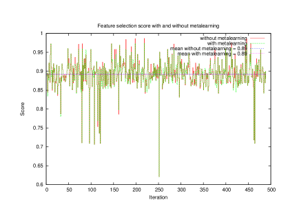
Figure 17: Feature selection scores for techtc500, $MI=0.05$, $FE=10000$, $t=0.2$

Figure 18: Learning scores for techtc500, $MI=0.05$, $FE=10000$, $t=0.2$

4.8 Metalearning Computational Cost

We have seen that the feature metalearning methodology is showing promise even for hard problem collections (hard due to the distant semantic between problems). However it remains to evaluate whether feature metalearning is worth it in term of computational cost. Here we present conclusions based on extrapolating from the computational cost of our experiments, run on an Intel Quad Core 2.5GHz, with feature selection parallelized over the 4 cores.

First, we measured that the computational cost of MetaDB maintenance is largely negligible as compared to feature selection – with the exception of the nearest neighbor querying process. Regarding the latter, we’ve represented in Figure 20 the computational time for nearest neighbor query, beside feature selection with and without metalearning, for the experiment detailed in Section 4.7, using our current implementation.

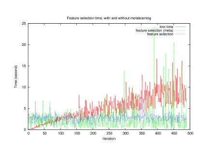
Figure 19: Computational time of metalearning for techtc500, $MI=0.05$, $FE=10000$, $t=0.2$

As shown in the figure, in our current implementation, the time spent for nearest neighbor query is not only significant but badly exceeds the time for feature selection. What this shows is that, in our current software implementation, feature metalearning is not practically useful. Fortunately, though, this is a function of the limitations of our current implementation, rather than reflecting a fundamental limitation of the algorithmic approach.

It is clear that the nearest neighbor query implementation in our current software is very far from optimal, as it was created solely to allow rapid experimentation with the feature metalearning methodology. For one thing, this part of our current feature metalearning pipeline has been entirely coded in Python, while feature selection is coded in C++ and the computation is spread over 4 cores. Considering that Python is at least 10x slower than C++ and that nearest neighbor query is running on a single core while feature selection is running on 4 cores the results shown in the figure are quite unfair. The following Figure shows the same graph but with nearest neighbor query time divided by $10\times 4=40$.

Figure 20: Computational time of metalearning for techtc500, $MI=0.05$, $FE=10000$, $t=0.2$

Here the estimated cost of metalearning maintenance is almost negligible but shows a linear increase which – if it continued – would eventually render the approach too costly. We conjecture that at some point the cover tree data structure used in the MetaDB will dampen the linear growth before the cost becomes intolerable. There are also other ways to address this problems, for instance one could consider datasets containing only the most relevant features instead of the entire dataset when initially calculating the JSD; and then only calculate the JSD on the entire datasets if the distance estimated over the filtered datasets goes under a certain threshold.

5 Conclusion and Future Directions

The results of our initial explorations in feature metalearning, presented here, are very promising in the sense that they demonstrate that the approach works. However, a lot of work remains to turn feature metalearning into a broadly powerful methodology.

Specifically, we have shown that, in the text classification context at least,

• If the collection of datasets is sufficiently ”dense”, in the sense that a dataset generally has some fairly close neighbors in dataset-space, then feature metalearning gives positive speedup and doesn’t degrade the quality of the final answer

• The speedup is greatest in the case where one needs a quick answer and doesn’t allocate enough time to the problem-solving process to find an optimal feature set, but only needs a ”best I can find in the time available” feature set

In order to work around the first limitation, we believe it will be necessary to replace nearest-neighbor search with a more sophisticated meta-level learning algorithm – perhaps, for instance, using evolutionary programming itself on the meta level, to learn patterns in which feature combinations tend to be effective on which problems.

In order to work around the second limitation, and perhaps to an extent the first as well, the following steps may be useful:

1. Improve the feature transfer formula. The one given in Section 3.3.2 is a rather crude heuristic; given more work we could improve its positive vs negative transfer ratio.

2. The more features allowed to be selected, the more likely positive transfer may occur. Here, again because running such large experiments takes a lot of time, the experiments were conducted with only a dozen features on average for each iteration. The typical number of features required to solve the family of problems we explored are more commonly around 50 and can go into hundreds.

It should also be noted that the problem collection we chose to work with is quite hard from a feature metalearning perspective, because the problems are semantically quite distant. For this among other obvious reasons, it would be nice to explore feature metalearning on a variety of different problem areas, not just supervised text classification of Web pages.

We believe the feature metalearning approach has great promise to dramatically accelerate machine learning in cases where there is a large number of relatively similar problems with features drawn from a common feature space. The initial algorithms reported here have sufficed to demonstrate the viability of the approach, and explore some of its properties. Refining them via future research should ultimately lead to the development of extremely powerful feature metalearning systems.

Acknowledgement

We would like to thank Andras Kornai for encouraging us to look at the problem of feature metalearning.

References

- [BCSV08] Pavel Brazdil, Christophe Giraud Carrier, Carlos Soares, and Ricardo Vilalta. Metalearning: Applications to Data Mining. Springer, 2008.
- [BKL06] Alina Beygelzimer, Sham Kakade, and John Langford. Cover trees for nearest neighbor. In ICML, pages 97–104, 2006.
- [Bla09] M Blachnik. Comparison of various feature selection methods in application to prototype best rules advanced in intelligent and soft computing. In Proc. of 6th Inter. Conf. on Comp. Recognition Systems, CORES’09, 2009.
- [DGM04] Dmitry Davidov, Evgeniy Gabrilovich, and Shaul Markovitch. Parameterized generation of labeled datasets for text categorization based on a hierarchical directory. In The 27th Annual International ACM SIGIR Conference, Sheffield, UK, July, pages 250–257, 2004.
- [DWBB09] W Duch, T Wieczorek, J Biesiada, and M Blachnik. Comparision of feature ranking methods based on information entropy. In Proc. of 6th Inter. Conf. on Comp. Recognition Systems, CORES’09, 2009.
- [Gab04] Evgeniy Gabrilovich. http://techtc.cs.technion.ac.il/techtc300/techtc300.html, 2004.
- [Gei11] Nil Geisweiller. https://github.com/ngeiswei/techtc-builder, 2011.
- [GIGH08] B Goertzel., M Ikle, I Goertzel, and A Heljakka. Probabilistic Logic Networks. Springer, 2008.
- [GSMP08] Ben Goertzel, Lucio Souza, Mauricio Mudado, and Cassio Pennachin. Identifying the genes and genetic interrelationships underlying the impact of calorie restriction on maximum lifespan: An artificial intelligence based approach. Rejuvenation Research, 2008.
- [KDBB10] A Kachel, W Duch, Blachnik, and M Biesiada. Infosel++: Information based feature selection c++ library. In ICAISC 2010,Lecture Notes in Artificial Intelligence, Vol. 6113, pages 388–396, 2010.
- [Loo06] Moshe Looks. Competent Program Evolution. PhD Thesis, Computer Science Department, Washington University, 2006.
- [Loo07] M. Looks. Scalable estimation-of-distribution program evolution. In Genetic and evolutionary computation conference, 2007.
- [Net] Netscape. http://www.dmoz.org.