Spectral equations for the modular oscillator

Abstract.

Motivated by applications for non-perturbative topological strings in toric Calabi–Yau manifolds, we discuss the spectral problem for a pair of commuting modular conjugate (in the sense of Faddeev) Harper type operators, corresponding to a special case of the quantized mirror curve of local $\mathbb{P}^{1}\times\mathbb{P}^{1}$ and complex values of Planck’s constant. We illustrate our analytical results by numerical calculations.

1. Introduction

Topological string theory is known for its prominent role in relating different subjects of mathematical physics and mathematics such as Chern–Simons theory, Gromov–Witten invariants, mirror symmetry, enumerative geometry, quantum topology, integrable systems, supersymmetric gauge theory, random matrix theory, etc. The recent progress in string theory has lead to remarkable connections between spectral theory, integrable systems and local mirror symmetry. The idea of relating topological strings in toric Calabi–Yau manifolds with quantum mechanical spectral problems originating from integrable systems was put forward in [1] and subsequently has been materialised to a powerful and numerically testable conjecture of Grassi–Hatsuda–Mariño [7]. It has been shown that quantization of mirror curves leads to trace class (one-dimensional) quantum mechanical operators, whose spectral properties not only contain the full information of the enumerative geometry of the underlying Calabi–Yau manifold, but also allow to formulate the string theory non-perturbatively, see [14] for a review and references therein. Outside the context of string theory, these results are preceded by connections of some quantum mechanical spectral problems with integrable systems and conformal field theory [4, 3].

In the case of toric Calabi–Yau threefold known as local $\mathbb{P}^{1}\times\mathbb{P}^{1}$ or local $\mathbb{F}_{0}$, the corresponding operator obtained from quantisation of the mirror curve is of the form

(1) $$\boldsymbol{O}_{\mathbb{F}_{0},m}=\boldsymbol{v}+\boldsymbol{v}^{-1}+\boldsymbol{u}+m\boldsymbol{u}^{-1}$$

with positive self-adjoint operators $\boldsymbol{u}$ and $\boldsymbol{v}$ satisfying the Heisenberg–Weyl commutation relation

(2) $$\boldsymbol{u}\boldsymbol{v}=\operatorname{{e}}^{\mathsf{i}\hbar}\boldsymbol{v}\boldsymbol{u},\quad\hbar\in\mathbb{R}_{>0},$$

and positive real parameter $m$. In the special case $m=1$, operator $\boldsymbol{O}_{\mathbb{F}_{0},1}$ structurally resembles the Harper operator [8], but the fact that operators $\boldsymbol{u}$ and $\boldsymbol{v}$ are positive self-adjoint rather than unitary makes its quantum mechanical content very different: it has purely discrete positive spectrum, and its inverse $\boldsymbol{O}_{\mathbb{F}_{0},m}^{-1}$ is of trace class [11, 12]. Nonetheless, recent findings in [9, 10] indicate to hidden connections of the two cases through Faddeev’s modular duality [5].

The spectral problem of operator (1) has been addressed in [16] as a part of a larger class of integrable systems related to supersymmetric gauge theories, and, more recently, in [13] from the perspective of exact WKB approximation and in [15] by using a matrix integral representation of the eigenfunctions. One can approach the same problem from the standpoint of quantum integrable systems by noting that both the Bethe ansatz equations and the quantum method of separation of variables can be formulated in more general and universal framework of Baxter’s $T-Q$ functional difference equations [2] which, in their turn, can be interpreted as (one-dimensional) quantum mechanical spectral problems. Complemented with Faddeev’s modular duality idea, the second-named author has shown in [17] that the modular $T-Q$ equations of general form admit a particularly tractable approach to their solution in the so called “strong coupling” regime corresponding to a complexified parameter $\hbar$ in the commutation relation (2), namely $\hbar=2\pi\operatorname{{e}}^{\mathsf{i}2\theta}$ with real $\theta\in]0,\pi/2[$. In this case, operators $\boldsymbol{u}$ and $\boldsymbol{v}$ cannot be neither self-adjoint nor unitary, but one can choose them to be normal and satisfying the relation

(3) $$\boldsymbol{u}\boldsymbol{v}^{\dagger}=\boldsymbol{v}^{\dagger}\boldsymbol{u},$$

implying that operator (1) stays normal, and thus its spectral problem still makes sense.

In this paper, motivated by topological string applications, we address the spectral problem of operator (1) in the special case $m=1$ and $\hbar=2\pi\operatorname{{e}}^{\mathsf{i}2\theta}$ with $\theta\in[0,\pi/2[$. Our approach is based on solving Baxter’s $T-Q$ equations in terms of analytic functions on the entire complex plane. The strong coupling regime $\theta\in]0,\pi/2[$ is treated along the approach of [17], while the case $\theta=0$ (corresponding to $\hbar=2\pi$) is treated by solving the functional difference equation directly. We illustrate our analytical results with numerical calculations.

The organisation of the paper is as follows. In Section 2 we formulate the problem, fix the notation and conventions. In Sections 3–6, we describe the solution of the problem in the strongly coupled regime. First, we introduce the main functional difference equation and describe some of its properties (Sec. 3), then we construct the eigenfunctions with minimal number of poles (Sec. 4), describe the spectral equations as conditions of cancelling the poles (Sec. 5), and give some numerical analysis in the special case $\hbar=2\pi\mathsf{i}$ (Sec. 6). In the final Section 7, we give a solution of the case $\hbar=2\pi$.

Acknowledgements

We would like thank Jørgen Ellegaard Andersen, Vladimir Bazhanov, Tobias Ekholm, Ludwig Faddeev, Vladimir Mangazeev, Marcos Mariño, Szabolc Zakany for valuable discussions. Our special thanks go to Alba Grassi, Marcos Mariño and Szabolc Zakany for sharing with us their results prior to publication. The work is partially supported by Australian Research Council, and the work of R.M.K. is partially supported by Swiss National Science Foundation.

2. Background from basic quantum mechanics

Let $\boldsymbol{x}$ and $\boldsymbol{p}$ be normalised self-adjoint quantum mechanical position and momentum operators in the Hilbert space $L^{2}(\mathbb{R})$ defined by the functional equalities

(4) $$\boldsymbol{x}\psi(x)=x\psi(x),\quad\boldsymbol{p}\psi(x)=\frac{1}{2\pi\mathsf{i}}\frac{\partial\psi(x)}{\partial x}$$

so that the Heisenberg commutation relation between them takes the form

(5) $$[\boldsymbol{p},\boldsymbol{x}]:=\boldsymbol{p}\boldsymbol{x}-\boldsymbol{x}\boldsymbol{p}=\frac{1}{2\pi\mathsf{i}},$$

i.e. with specific choice of Planck’s constant $h=2\pi\hbar=1$. As these are unbounded operators, it is assumed that the function $\psi(x)$ in (4) is taken from the respective domains $D(\boldsymbol{x})$ and $D(\boldsymbol{p})$.

For each non-zero complex parameter $\mathsf{b}$, there are two pairs of exponential operators

(6) $$\boldsymbol{u}:=\operatorname{{e}}^{2\pi\mathsf{b}\boldsymbol{x}}\;,\quad\boldsymbol{v}:=\operatorname{{e}}^{2\pi\mathsf{b}\boldsymbol{p}}\;,$$

and

(7) $$\bar{\boldsymbol{u}}:=\operatorname{{e}}^{2\pi\mathsf{b}^{-1}\boldsymbol{x}}\;,\quad\bar{\boldsymbol{v}}:=\operatorname{{e}}^{2\pi\mathsf{b}^{-1}\boldsymbol{p}}\;,$$

which satisfy the Weyl commutations relations

(8) $$\boldsymbol{u}\boldsymbol{v}=q^{2}\boldsymbol{v}\boldsymbol{u}\;,\quad\bar{\boldsymbol{v}}\bar{\boldsymbol{u}}=\bar{q}^{2}\bar{\boldsymbol{u}}\bar{\boldsymbol{v}}\;,$$

where

(9) $$q:=\operatorname{{e}}^{\mathsf{i}\pi\mathsf{b}^{2}}\;,\quad\bar{q}:=\operatorname{{e}}^{-\mathsf{i}\pi\mathsf{b}^{-2}}\;,$$

and all other commutation relations are trivial. In coordinate representation (4), we have

(10) $$\boldsymbol{u}\psi(x)=\operatorname{{e}}^{2\pi\mathsf{b}x}\psi(x),\quad\boldsymbol{v}\psi(x)=\psi(x-\mathsf{i}\mathsf{b}),$$

and

(11) $$\bar{\boldsymbol{u}}\psi(x)=\operatorname{{e}}^{2\pi\mathsf{b}^{-1}x}\psi(x),\quad\bar{\boldsymbol{v}}\psi(x)=\psi(x-\mathsf{i}\mathsf{b}^{-1}).$$

The case where parameter $\mathsf{b}$ is pure imaginary corresponds to unitary exponentials, while in this paper we will mainly assume the strong coupling regime

(12) $$\mathsf{b}=\operatorname{{e}}^{\mathsf{i}\theta}\;,\quad\theta\in]0,\pi/2[\;\subset\mathbb{R},$$

which corresponds to unbounded exponentials. In this latter case, the operation bar in (7)–(9) and (11) is the complex conjugation for numbers and Hermitian conjugation for operators. We will keep that notation in a broader context of analytically continued parameters and variables always assuming that

(13) $$|q|<1\quad\Leftrightarrow\quad\Im\mathsf{b}^{2}>0\quad\Leftrightarrow\quad|\bar{q}|<1\;.$$

As in (4), the function $\psi(x)$ in (10) and (11) is assumed to belong to respective domains of unbounded operators. For example, the domain of operator $\boldsymbol{v}$ consists of analytic functions in the open strip between the real axis $\mathbb{R}\subset\mathbb{C}$ and the line $-\mathsf{i}\mathsf{b}+\mathbb{R}$, which are continuous on the closure of the strip, and which restrict to square integrable functions on the boundary of the strip.

We remark that the simultaneous appearance in a theory of both pairs of exponential operators (6) and (7) is a manifestation of Faddeev’s modular duality [5].

Statement of the problem

We address the spectral problem of the following pair of commuting operators (to be called Hamiltonians):

(14) $$\boldsymbol{H}=\boldsymbol{v}+\boldsymbol{v}^{-1}+\boldsymbol{u}+\boldsymbol{u}^{-1},\quad\bar{\boldsymbol{H}}=\bar{\boldsymbol{v}}+\bar{\boldsymbol{v}}^{-1}+\bar{\boldsymbol{u}}+\bar{\boldsymbol{u}}^{-1}\;.$$

In the strong coupling regime (12), $\bar{\boldsymbol{H}}=\boldsymbol{H}^{\dagger}$ so that commutativity of $\boldsymbol{H}$ and $\bar{\boldsymbol{H}}$ means that $\boldsymbol{H}$ is a normal operator. In the coordinate representation (4), the spectral problems

(15) $$\boldsymbol{H}\psi=\varepsilon\psi,\quad\bar{\boldsymbol{H}}\psi=\bar{\varepsilon}\psi$$

correspond to the following pair of functional difference equations:

(16) $$\psi(x+\mathsf{i}\mathsf{b})+\psi(x-\mathsf{i}\mathsf{b}) =(\varepsilon-2\cosh(2\pi\mathsf{b}x))\psi(x),$$

(17) $$\psi\left(x-\mathsf{i}\mathsf{b}^{-1}\right)+\psi\left(x+\mathsf{i}\mathsf{b}^{-1}\right) =(\bar{\varepsilon}-2\cosh(2\pi\mathsf{b}^{-1}x))\psi(x).$$

By definition, solving these spectral problems corresponds to construction of a function $\psi(x)$ and determination of specific values of $\varepsilon$ and $\bar{\varepsilon}$ such that

1. $\psi(x)$ is analytic in an open strip around the real axis whose closure contains $\pm\mathsf{i}\mathsf{b}$ and $\pm\mathsf{i}\mathsf{b}^{-1}$, and it is continuous on the closure of that strip;

2. $\psi(x)$ is square integrable on the real axis and all of its translates by $\pm\mathsf{i}\mathsf{b}$ and $\pm\mathsf{i}\mathsf{b}^{-1}$;

3. equations (16), (17) are satisfied for all $x\in\mathbb{R}$.

Remark 1.

As we will see, the solution of the spectral problems (16), (17) is given by analytic functions on the entire complex plane.

Conventions. Throughout the text, each time when we use the variables $u$, $\bar{u}$ and $x$, we assume that they are related as follows:

(18) $$u=\operatorname{{e}}^{2\pi\mathsf{b}x}\;,\quad\bar{u}=\operatorname{{e}}^{2\pi x/\mathsf{b}}\;.$$

Similarly, as soon as we use the variables $s$, $\bar{s}$ and $\sigma$, we assume that they are related as follows:

(19) $$s=\operatorname{{e}}^{2\pi\mathsf{b}\sigma}\;,\quad\bar{s}=\operatorname{{e}}^{2\pi\sigma/\mathsf{b}}\;.$$

Else, if $\displaystyle f=f(u,\varepsilon,q)$, then we write $\displaystyle\bar{f}=\overline{f(u,\varepsilon,q)}$ meaning the analytic continuation of the complex conjugation in the strong coupling regime.

Remark 2.

In the limit $\mathsf{b}\to 0$ one has

(20) $$\boldsymbol{H}=4+(2\pi\mathsf{b})^{2}(\boldsymbol{p}^{2}+\boldsymbol{x}^{2})+\mathcal{O}(\mathsf{b}^{4})\;,$$

what justifies the term “oscillator”.

3. The main functional equation

In this section, we study the following functional finite difference equation

(21) $$f\left(\frac{u}{q^{2}}\right)+q^{2}u^{2}f(q^{2}u)=(1-\varepsilon u+u^{2})f(u).$$

We can rewrite it as a first order difference matrix equation

(22) $$\left(\begin{array}[]{cc}f\left(\frac{u}{q^{2}}\right)\\ f(u)\end{array}\right)\;=\;L(u)\left(\begin{array}[]{cc}f\left(u\right)\\ f(q^{2}u)\end{array}\right)$$

where

(23) $$L(u):=\left(\begin{array}[]{cc}\displaystyle 1-\varepsilon u+u^{2}&\displaystyle-q^{2}u^{2}\\ \displaystyle 1&\displaystyle 0\end{array}\right).$$

Upon iteration of (22), we obtain

(24) $$\left(\begin{array}[]{cc}f\left(\frac{u}{q^{2}}\right)\\ f(u)\end{array}\right)\;=\;M_{n}(u)\left(\begin{array}[]{cc}f\left(q^{2n-2}u\right)\\ f(q^{2n}u)\end{array}\right),\quad\forall n\in\mathbb{Z}_{>0},$$

where

(25) $$M_{n}(u):=L(u)L(q^{2}u)\cdots L(q^{2(n-1)}u)$$

is a sequence of matrix valued polynomials in $u$ (the degree of $M_{n}(u)$ is $2n$) which satisfies the following obvious relations

(26) $$M_{m+n}(u)=M_{m}(u)M_{n}(q^{2m}u),\quad\forall m,n\in\mathbb{Z}_{\geq 0}.$$

3.1. The regular solution $\boldsymbol{\chi}_{q}(u,\varepsilon)$

The limit $n\to\infty$ leads to a matrix valued entire function $M_{\infty}(u)$, i.e. a holomorphic function on the entire complex plane of the variable $u$. This follows from the following functional analytic argument.

For any $r\in\mathbb{R}_{>0}$, let $V_{r}$ be the vector space of $\mathbb{C}^{2}$-valued continuous functions on the closed disk

(27) $$D_{r}:=\{z\in\mathbb{C}\ |\ |z|\leq r\}.$$

It is a Banach space with respect to the norm

(28) $$\|g\|_{r}:=\max_{z\in D_{r}}\|g(z)\|,\quad\|g(z)\|:=\max_{i\in\{1,2\}}|g_{i}(z)|,\quad\forall g\in V_{r}.$$

We have the following monotonicity property of the norms with different disk radii:

(29) $$s\leq r\quad\Rightarrow\quad\left\|g|_{D_{s}}\right\|_{s}\leq\|g\|_{r},\quad\forall g\in V_{r}.$$

Lemma 1.

For any $r\in\mathbb{R}_{>0}$, the sequence of restrictions $M_{n}|_{D_{r}}$, $n\in\mathbb{Z}_{n>0}$, forms a (fundamental) Cauchy sequence with respect to the induced norm in the (Banach) algebra of bounded linear operators over $V_{r}$.

Proof.

On the level of matrix valued continuous functions $A\colon D_{r}\to\operatorname{End}(\mathbb{C}^{2})$, the induced norm is calculated as follows:

(30) $$\|A\|_{r}=\max_{z\in D_{r}}\|A(z)\|,\quad\|A(z)\|:=\max_{i\in\{1,2\}}\sum_{j=1}^{2}|A_{i,j}(z)|.$$

Using this formula and the explicit form (23) of the polynomial matrix $L(u)$, we have

(31) $$\|L\|_{r}\geq 1,\quad\forall r\in\mathbb{R}_{\geq 0},$$

and

(32) $$\|L\|_{r}\leq 1+r(r+1)T,\quad T:=\max_{i\in\{1,2\}}\|L_{i}\|\geq 1+|q|^{2},$$

where $L_{i}\in\operatorname{End}(\mathbb{C}^{2})$ are the expansion coefficients of the matrix $L(u)$:

(33) $$L(u)=\sum_{i=0}^{2}L_{i}u^{i},$$

the coefficient $L_{0}=L(0)$ being a projection matrix of unit norm:

(34) $$L_{0}^{2}=L_{0},\quad\|L_{0}\|=1.$$

That allows us to get a uniform in $m$ upper bound for the norms of $M_{m}(u)$:

(35) $$\|M_{m}\|_{r}\leq\max_{z\in D_{r}}\prod_{i=0}^{m-1}\|L(zq^{2i})\|\leq\prod_{i=0}^{m-1}\|L\|_{r|q|^{2i}}\leq\prod_{i=0}^{\infty}\|L\|_{r|q|^{2i}}=:\nu(r),$$

where the infinite product converges due to inequality (32). On the other hand, the norms of the coefficients in the expansions

(36) $$M_{m}(u)=\sum_{k=0}^{2m}M_{m,k}u^{k},\quad M_{m,k}:=\sum_{\begin{subarray}{c}0\leq i_{1},\dots,i_{m}\leq 2\\ i_{1}+\dots+i_{m}=k\end{subarray}}L_{i_{1}}\dots L_{i_{m}}q^{2\sum_{j=1}^{m-1}ji_{j+1}}.$$

are also bounded from above uniformly on $m$:

(37) $$\|M_{m,k}\|\leq\sum_{\begin{subarray}{c}0\leq i_{1},\dots,i_{m}\leq 2\\ i_{1}+\dots+i_{m}=k\end{subarray}}\|L_{i_{1}}\|\dots\|L_{i_{m}}\||q|^{2\sum_{j=1}^{m-1}ji_{j+1}}\leq\frac{3T^{k}}{(|q|^{2};|q|^{2})_{m-1}}\leq\frac{3T^{k}}{(|q|^{2};|q|^{2})_{\infty}}$$

with the standard notation for the deformed Pochhammer symbols

(38) $$(x;q)_{n}:=\prod_{i=0}^{n-1}(1-xq^{i}).$$

For any $m,n\in\mathbb{Z}_{>0}$, there exists a matrix valued polynomial $A_{m,n}(u)$ of degree $2\max(m,n)-1$ such that

(39) $$M_{m}(u)-M_{n}(u)=uA_{m,n}(u).$$

Explicitly, we have

(40) $$A_{m,n}(u)=\sum_{k=0}^{2\max(m,n)-1}(M_{m,k}-M_{n,k})u^{k}$$

so that

(41) $$\|A_{m,n}\|_{r}\leq\sum_{k=0}^{2\max(m,n)-1}(\|M_{m,k}\|+\|M_{n,k}\|)r^{k}\leq\frac{6\left(1-(rT)^{2\max(m,n)}\right)}{(|q|^{2};|q|^{2})_{\infty}(1-rT)}.$$

Let $N_{r}\in\mathbb{Z}_{>0}$ be such that $rT|q|^{2N_{r}}<1$. Then for any $m\geq N_{r}$ and $n\geq 0$, taking into account the formula

(42) $$M_{m+n+1}(u)-M_{m+1}(u)=M_{m}(u)uq^{2m}A_{n+1,1}(uq^{2m})$$

and the inequalities (35) and (41), we obtain

(43) $$\|M_{m+n+1}-M_{m+1}\|_{r}\leq|q|^{2m}r\|M_{m}\|_{r}\|A_{n+1,1}\|_{r|q|^{2m}}\\ \leq|q|^{2m}r\nu(r)\frac{6(1-(rT|q|^{2m})^{2n+2})}{(|q|^{2};|q|^{2})_{\infty}(1-rT|q|^{2m})}\leq|q|^{2m}\frac{6r\nu(r)}{(|q|^{2};|q|^{2})_{\infty}(1-rT|q|^{2N_{r}})}$$

The obtained equality implies that $(M_{m}|_{D_{r}})_{m>0}$ is a Cauchy sequence in the Banach algebra of bounded linear operators over $V_{r}$. ∎

Lemma 1 implies the uniform convergence of the matrix coefficients of $M_{n}(u)$ on all compact subsets of $\mathbb{C}$. Indeed , let $f_{n}(u)$ be a matrix element of $M_{n}(u)$ and $K\subset\mathbb{C}$ a compact set. Then there exists $r\in\mathbb{R}_{>0}$ such that $K\subset D_{r}$ and thus

(44) $$|f_{m}(u)-f_{n}(u)|\leq\|M_{m}(u)-M_{n}(u)\|\leq\|M_{m}-M_{n}\|_{r},\quad\forall u\in K.$$

Thus, $M_{\infty}(u)$ is an entire function on $\mathbb{C}$ as a uniformly convergent limit on all compact subsets of $\mathbb{C}$ of a sequence of polynomial functions.

By taking into account the equalities

(45) $$M_{\infty}(u)=L(u)M_{\infty}(q^{2}u)=M_{\infty}(u)L(0),\quad M_{\infty}(0)=L(0),$$

we immediately arrive to the following structure of the matrix $M_{\infty}(u)$:

(46) $$M_{\infty}(u)=\left(\begin{array}[]{cc}\displaystyle\boldsymbol{\chi}_{q}\left(q^{-2}u\right)&\displaystyle 0\\ \displaystyle\boldsymbol{\chi}_{q}(u)&\displaystyle 0\end{array}\right),$$

where $\boldsymbol{\chi}_{q}(u)=\boldsymbol{\chi}_{q}(u,\varepsilon)$ is an entire function normalised so that $\boldsymbol{\chi}_{q}(0)=1$ and which solves the functional difference equation (21). On the other hand, if write

(47) $$M_{n}(u)=\left(\begin{array}[]{cc}\displaystyle a_{n}(u)&\displaystyle b_{n}(u)\\ \displaystyle c_{n}(u)&\displaystyle d_{n}(u)\end{array}\right),$$

then the matrix equality

(48) $$L(u)M_{n}(q^{2}u)=M_{n}(u)L(q^{2n}u)$$

implies that

(49) $$b_{n}(q^{2}u)=-q^{4n+2}u^{2}c_{n}(u),\quad d_{n}(q^{2}u)=q^{4n}(a_{n}(u)-(1-\varepsilon u+u^{2})c_{n}(u)),$$

and we explicitly see the rate at which $b_{n}(u)$ and $d_{n}(u)$ converge to zero functions. Furthermore, by taking into account the limits

(50) $$\lim_{n\to\infty}a_{n}(u)=\boldsymbol{\chi}_{q}(q^{-2}u),\quad\lim_{n\to\infty}c_{n}(u)=\boldsymbol{\chi}_{q}(u),$$

we obtain from (49)

(51) $$\lim_{n\to\infty}q^{-4n}b_{n}(u)=-q^{-2}u^{2}\boldsymbol{\chi}_{q}(q^{-2}u),\quad\lim_{n\to\infty}q^{-4n}d_{n}(u)=-q^{-2}u^{2}\boldsymbol{\chi}_{q}(u),$$

where in the last limit we have used the equation (21) for $\boldsymbol{\chi}_{q}(u)$.

Theorem 1 (Uniqueness of the regular solution).

In the case $|q|<1$, let $f(u)$ be a solution of the functional equation (21) which is regular (i.e. holomorphic) at $u=0$ and normalised so that $f(0)=1$. Then $f(u)=\boldsymbol{\chi}_{q}(u)$.

Proof.

Taking the limit $n\to\infty$ in the matrix equality (24) and using the regularity and normalisation properties of $f(u)$ at $u=0$, we obtain the equality

(52) $$\left(\begin{array}[]{cc}f\left(q^{-2}u\right)\\ f(u)\end{array}\right)=M_{\infty}(u)\left(\begin{array}[]{cc}1\\ 1\end{array}\right)=\left(\begin{array}[]{cc}\boldsymbol{\chi}_{q}\left(q^{-2}u\right)\\ \boldsymbol{\chi}_{q}(u)\end{array}\right).$$

∎

Lemma 2.

In the space of solutions of (21), there is an involution which associates to any solution $f(u)$ another solution $\check{f}(u)$ defined by

(53) $$\check{f}(u)=u^{-1}f\left(u^{-1}\right).$$

Proof.

This is an easy direct verification. ∎

Applying Lemma 2 to our regular solution $\boldsymbol{\chi}_{q}(u,\varepsilon)$, we obtain a second solution of the recursion equation (21)

(54) $$\check{\boldsymbol{\chi}}_{q}(u,\varepsilon):=u^{-1}\boldsymbol{\chi}_{q}(u^{-1},\varepsilon)$$

which is holomorphic in $\mathbb{C}_{\neq 0}$.

3.2. Orthogonal polynomials associated to $\boldsymbol{\chi}_{q}(u,\varepsilon)$

The function $\boldsymbol{\chi}_{q}(u,\varepsilon)$ can be expanded as a power series

(55) $$\boldsymbol{\chi}_{q}(u,\varepsilon)=\sum_{n\geq 0}c_{n}u^{n},\quad c_{0}=1,$$

with infinite radius of convergence. The coefficients here are functions of $\varepsilon$ and $q$. The functional equation (21) in this case is translated into a system of recurrence equations on the coefficients

(56) $$(1-q^{-2-2n})c_{n+1}=\varepsilon c_{n}-(1-q^{2n})c_{n-1},\quad n\in\mathbb{Z}_{\geq 0},$$

which, upon multiplication by $(q^{-2};q^{-2})_{n}$, is rewritten as a system of recurrence relations defining orthogonal polynomials $\chi_{q,n}(\varepsilon)\in\mathbb{C}[\varepsilon]$, $n\in\mathbb{Z}_{n\geq 0}$:

(57) $$\chi_{q,0}(\varepsilon)=1\;,\quad\chi_{q,n+1}(\varepsilon)=\varepsilon\chi_{q,n}(\varepsilon)+(q^{n}-q^{-n})^{2}\chi_{q,n-1}(\varepsilon),$$

where

(58) $$\chi_{q,n}(\varepsilon):=(q^{-2};q^{-2})_{n}c_{n}.$$

Notice that the polynomials $\chi_{q,n}(\varepsilon)$ also depend on the deformation parameter $q$ in symmetric way in the sense that they are unchanged under the replacement $q\mapsto q^{-1}$. Here are the explicit forms of the first four polynomials

(59) $$\chi_{q,0}(\varepsilon)=1,\quad\chi_{q,1}(\varepsilon)=\varepsilon,\quad\chi_{q,2}(\varepsilon)=\varepsilon^{2}+(q-q^{-1})^{2},\\ \chi_{q,3}(\varepsilon)=\varepsilon(\varepsilon^{2}+(q^{2}-q^{-2})^{2}+(q-q^{-1})^{2}),\quad\ldots$$

Thus, our solution $\boldsymbol{\chi}_{q}(u,\varepsilon)$ is represented in the form of a power series

(60) $$\boldsymbol{\chi}_{q}(u,\varepsilon)\;:=\;\sum_{n\geq 0}\frac{\chi_{q,n}(\varepsilon)}{(q^{-2};q^{-2})_{n}}u^{n}=\sum_{n\geq 0}(-1)^{n}q^{n(n+1)}\frac{\chi_{q,n}(\varepsilon)}{(q^{2};q^{2})_{n}}u^{n}\;.$$

In order to see explicitly how this series absolutely convergences on the entire complex plane of the variable $u$, it suffices to find the growth rate of the polynomials $\chi_{q,n}(\varepsilon)$ at large index $n$. To this end, we observe that the recurrence relation (57) at large $n$ approaches the form

(61) $$\chi_{n+1}\simeq\varepsilon\chi_{n}+q^{-2n}\chi_{n-1}$$

where we have suppressed the arguments $q$ and $\varepsilon$ of $\chi_{q,n}(\varepsilon)$ and have taken into account the inequality $|q|<1$. This equivalently can be rewritten as follows:

(62) $$\frac{\chi_{n+1}}{\chi_{n}}\frac{\chi_{n}}{\chi_{n-1}}\simeq\varepsilon\frac{\chi_{n}}{\chi_{n-1}}+q^{-2n}\\ \quad\Leftrightarrow\quad\frac{\chi_{n}}{\chi_{n-1}}\simeq q^{-n}\quad\Leftrightarrow\quad\chi_{n}\simeq q^{-n^{2}/2}.$$

The latter relation immediately implies the absolute convergence of the sum in (60).

Theorem 2.

The orthogonal polynomials $\chi_{q,n}(\varepsilon)$ satisfy the following multiplication rules

(63) $$\chi_{q,m}(\varepsilon)\chi_{q,n}(\varepsilon)=\sum_{k=0}^{\min(m,n)}\frac{(q^{2m};q^{-2})_{k}(q^{2n};q^{-2})_{k}(q^{2(k-m-n)};q^{2})_{k}}{(q^{2};q^{2})_{k}}\chi_{q,m+n-2k}(\varepsilon)$$

Proof.

This is a direct check by recurrence on $\max(m,n)$. ∎

3.3. Non-linear first order functional difference equations

The vector space of solutions of (21) is a module over the algebra of $q^{2}$-periodic functions, i.e. functions $g(u)$ that satisfy the functional difference equation $g(q^{2}u)=g(u)$. For any nontrivial solution $f(u)$ of (21), the combinations

(64) $$R_{f}(u):=\frac{f(q^{-2}u)}{f(u)}$$

and

(65) $$P_{f}(u):=\frac{q^{2}u^{2}f(q^{2}u)}{f(u)}$$

are invariant with respect to multiplication by $q^{2}$-periodic functions, so that they can be used for characterisation of the equivalence classes of solutions of (21) differing by $q^{2}$-periodic functions. The two combinations are related to each other through the functional equalities

(66) $$P_{f}(u)R_{f}(q^{2}u)=q^{2}u^{2},\quad P_{f}(u)+R_{f}(u)=1-\varepsilon u+u^{2}.$$

The second order functional linear difference equation (21) implies first order non-linear functional difference equations for $R(u)=R_{f}(u)$

(67) $$R(u)R\left(q^{2}u\right)=(1-\varepsilon u+u^{2})R\left(q^{2}u\right)-q^{2}u^{2}$$

and for $P(u)=P_{f}(u)$

(68) $$P(u)P\left(q^{-2}u\right)=(1-\varepsilon u+u^{2})P\left(q^{-2}u\right)-q^{-2}u^{2}.$$

Notice that two equations are related to each other by the symmetry $q\mapsto q^{-1}$.

By using (24) and (47) we easily obtain the following linear fractional transformation formulae

(69) $$R(q^{2n}u)=\frac{d_{n}(u)R(u)-b_{n}(u)}{a_{n}(u)-c_{n}(u)R(u)},\quad\forall n\in\mathbb{Z}_{\geq 0}.$$

Theorem 3.

Let $R,P\colon U\to\mathbb{C}$, $U\subset\mathbb{C}$, be solutions of (67) and (68), respectively, and $z\in U$ be such that $\boldsymbol{\chi}_{q}(z)\neq 0$. Then the sequences $(R(q^{2n}z))_{n\geq 0}$ and $(P(q^{2n}z))_{n\geq 0}$ converge with the limits

(70) $$\lim_{n\to\infty}R(q^{2n}z)=\left\{\begin{array}[]{cc}0&\text{if}\ R(z)\neq R_{\boldsymbol{\chi}_{q}}(z);\\ 1&\text{otherwise.}\end{array}\right.$$

and

(71) $$\lim_{n\to\infty}P(q^{2n}z)=\left\{\begin{array}[]{cc}1&\text{if}\ P(z)\neq P_{\boldsymbol{\chi}_{q}}(z);\\ 0&\text{otherwise.}\end{array}\right.$$

Proof.

Formula (71) follows from (70) if we define $R(u):=1-\varepsilon u+u^{2}-P(u)$.

If $R(z)=R_{\boldsymbol{\chi}_{q}}(z)$, then formula (69) with $u=z$ implies that $R(q^{2n}z)=R_{\boldsymbol{\chi}_{q}}(q^{2n}z)$ for all $n\in\mathbb{Z}_{\geq 0}$. Thus,

(72) $$\lim_{n\to\infty}R(q^{2n}z)=\lim_{n\to\infty}R_{\boldsymbol{\chi}_{q}}(q^{2n}z)=R_{\boldsymbol{\chi}_{q}}(0)=1$$

by the regularity and the normalisation properties of $\boldsymbol{\chi}_{q}(u)$ at $u=0$.

If we assume that $R(z)\neq R_{\boldsymbol{\chi}_{q}}(z)$, then in equality (69) with $u=z$ the denominator is distinct from zero for sufficiently large $n$ since it converges to a nonzero number:

(73) $$\lim_{n\to\infty}(a_{n}(z)-c_{n}(z)R(z))=a_{\infty}(z)-c_{\infty}(z)R(z)=\boldsymbol{\chi}_{q}(q^{-2}z)-\boldsymbol{\chi}_{q}(z)R(z)=\boldsymbol{\chi}_{q}(z)(R_{\boldsymbol{\chi}_{q}}(z)-R(z)),$$

while the numerator converges to $b_{\infty}(z)R(z)-d_{\infty}(z)=0$. ∎

3.4. Wronskian of two solutions of the main functional equation

An important function associated with any two solutions of the functional equation (21) is their Wronskian or, more precisely, the functional difference analogue of the Wronskian in the theory of linear second order ordinary differentian equations. As we will see below, any Wronskian satisfies a particularly simple difference equation of the form

(74) $$W(q^{2}u)\;=\;\frac{1}{q^{2}u^{2}}W(u)\quad\Leftrightarrow\quad W\left(u/q\right)=u^{2}W(qu).$$

Definition-Proposition 1.

Let $f(u)$ and $g(u)$ satisfy equation (21). Then their Wronskian $[f,g](u)$ defined by

(75) $$[f,g](u):=f\left(q^{-2}u\right)g(u)-g\left(q^{-2}u\right)f(u)$$

satisfies equation (74).

Proof.

Substructing (21) for $g(u)$ multiplied by $f(u)$ from (21) for $f(u)$ multiplied by $g(u)$, we obtain

(76) $$\left(f\left(q^{-2}u\right)+q^{2}u^{2}f(q^{2}u)\right)g(u)=\left(g\left(q^{-2}u\right)+q^{2}u^{2}g(q^{2}u)\right)f(u)\\ \Leftrightarrow f\left(q^{-2}u\right)g(u)-g\left(q^{-2}u\right)f(u)=q^{2}u^{2}\left(g(q^{2}u)f(u)-f(q^{2}u)g(u)\right)\\ \Leftrightarrow[f,g](u)=q^{2}u^{2}[f,g](q^{2}u).$$

∎

Of particular importance for the sequel will be the Wronskian of $\boldsymbol{\chi}$ and $\check{\boldsymbol{\chi}}$:

(77) $$[\boldsymbol{\chi},\check{\boldsymbol{\chi}}](u)\;=\;\boldsymbol{\chi}\left(q^{-2}u\right)\check{\boldsymbol{\chi}}(u)-\check{\boldsymbol{\chi}}\left(q^{-2}u\right)\boldsymbol{\chi}(u)\;.$$

Here and hereafter we shorten the notation $\boldsymbol{\chi}(u)=\boldsymbol{\chi}_{q}(u,\varepsilon)$ and so on.

Lemma 3.

The Wronskian $[\boldsymbol{\chi},\check{\boldsymbol{\chi}}]$ is not the identically zero function.

Proof.

Using the power series expansions, we obtain a Laurent series

(78) $$[\boldsymbol{\chi},\check{\boldsymbol{\chi}}](u)=\sum_{n\in\mathbb{Z}}[\boldsymbol{\chi},\check{\boldsymbol{\chi}}]_{n}u^{n},$$

where the residue $[\boldsymbol{\chi},\check{\boldsymbol{\chi}}]_{-1}$ is given explicitly by the absolutely convergent series

(79) $$[\boldsymbol{\chi},\check{\boldsymbol{\chi}}]_{-1}=\sum_{m\geq 0}\left(\frac{\chi_{q,m}(\varepsilon)}{(q^{-2};q^{-2})_{m}}\right)^{2}(q^{-2m}-q^{2m+2})$$

where each term is non-negative if the variables $\varepsilon$ and $q$ are real with $0<q<1$. Thus, dropping all but the very first term, we obtain

(80) $$[\boldsymbol{\chi},\check{\boldsymbol{\chi}}]_{-1}\geq 1-q^{2}>0.$$

∎

3.5. Parameterization in terms of $\theta$-functions

Consider Jacobi’s $\theta$-function

(81) $$\theta_{1}(u,q)=\frac{1}{\mathsf{i}}\sum_{n\in\mathbb{Z}}(-1)^{n}q^{(n+1/2)^{2}}u^{n+1/2}\;.$$

It has the properties

(82) $$\theta_{1}(1,q)=0,\quad\theta_{1}(u^{-1},q)=-\theta_{1}(u,q),\quad\theta_{1}(q^{2}u,q)=-\frac{1}{qu}\theta_{1}(u,q),$$

and

(83) $$\overline{\theta_{1}(u,q)}=\mathsf{b}\operatorname{{e}}^{\pi\mathsf{i}/4-\mathsf{i}\pi x^{2}}\theta_{1}(u,q).$$

Any solution $W(u)$ of (74) in the form of a Laurent series in $u$, can be brought to the form

(84) $$W(u)=\varrho\theta_{1}(su,q)\theta_{1}(s^{-1}u,q).$$

for some constants $s$ and $\varrho$. The properties of the $\theta$-function given by (82) and (83) imply that

(85) $$\overline{W(u)}=\mathsf{i}\mathsf{b}^{2}\bar{\varrho}\varrho^{-1}\operatorname{{e}}^{-2\pi\mathsf{i}(\sigma^{2}+x^{2})}W(u),\quad u=\operatorname{{e}}^{2\pi\mathsf{b}x},\quad s=\operatorname{{e}}^{2\pi\mathsf{b}\sigma}.$$

In the case when $W=[\boldsymbol{\chi},\check{\boldsymbol{\chi}}]$, the variables $s$ and $\varrho$ will be determined in terms of $\varepsilon$ and $q$:

(86) $$s=s(\varepsilon,q),\quad\varrho=\varrho(\varepsilon,q).$$

The first of these dependences is of particular importance for us, and it will be the subject of a numerical study.

3.6. The main functional equation with $q$ replaced by $q^{-1}$

We turn now to the discussion of the functional equation (21) with $q$ replaced by $q^{-1}$:

(87) $$f(q^{2}u)+\frac{u^{2}}{q^{2}}f\left(\frac{u}{q^{2}}\right)=(1-\varepsilon u+u^{2})f(u)\;.$$

Let $\boldsymbol{\chi}_{q^{-1}}(u,\varepsilon)$ be the normalised solution (60) with $q$ replaced by $q^{-1}$, i.e. a power series of the form

(88) $$\boldsymbol{\chi}_{q^{-1}}(u,\varepsilon)\;\simeq\;\sum_{n\geq 0}\frac{\chi_{q,n}(\varepsilon)}{(q^{2};q^{2})_{n}}u^{n}$$

where we use the semi-equality symbol $\simeq$ to indicate the fact that the series is now only a formal power series as it has zero radius of convergence. This is an immediate consequence of the asymptotic behaviour of $\chi_{q,n}(\varepsilon)$ at large $n$ given by (62). Thus, there does not exist a regular at $u=0$ solution of equation (87). Nonetheless, the formal power series solution (88) is interpreted as the asymptotic expansion of a true solution which is not analytic at $u=0$. Before formulating this result we do some preparatory work.

Lemma 4.

Let $f(u)$ and $W(u)$ satisfy the functional equations (21) and (74) respectively. Then the ratio $f(u)/W(u)$ satisfies (87).

Proof.

This is a direct verification. ∎

Lemma 5.

Let $f(u)$ and $g(u)$ satisfy the functional equations (21) and (87) respectively. Then the combination

(89) $$\langle f,g\rangle(u):=f\left(\frac{u}{q^{2}}\right)g(u)-\frac{u^{2}}{q^{2}}g\left(\frac{u}{q^{2}}\right)f(u)$$

is $q^{2}$-periodic, i.e.

(90) $$\langle f,g\rangle(u)=\langle f,g\rangle(q^{2}u),\quad\forall u.$$

Proof.

Substructing (87) multiplied by $f(u)$ from (21) multiplied by $g(u)$ , we obtain

(91) $$\left(f\left(\frac{u}{q^{2}}\right)+q^{2}u^{2}f(q^{2}u)\right)g(u)=\left(g(q^{2}u)+\frac{u^{2}}{q^{2}}g\left(\frac{u}{q^{2}}\right)\right)f(u)\\ \Leftrightarrow f\left(\frac{u}{q^{2}}\right)g(u)-\frac{u^{2}}{q^{2}}g\left(\frac{u}{q^{2}}\right)f(u)=f(u)g(q^{2}u)-q^{2}u^{2}g(u)f(q^{2}u)$$

where the latter equality is exactly (90). ∎

Theorem 4.

The formal power series (88) is the asymptotic expansion of the following solution of the functional equation (87)

(92) $$\boldsymbol{\chi}_{q^{-1}}(u,\varepsilon):=\frac{\check{\boldsymbol{\chi}}_{q}(u,\varepsilon)}{[\boldsymbol{\chi}_{q},\check{\boldsymbol{\chi}}_{q}](u)}\;$$

where the Wronskian $[\boldsymbol{\chi}_{q},\check{\boldsymbol{\chi}}_{q}](u)$ is defined in (77).

Proof.

The fact that $\boldsymbol{\chi}_{q^{-1}}(u,\varepsilon)$ defined in (92) satisfies (87) follows from Lemma 4. The rest of the proof is based on the following two easily verifiable functional identities

(93) $$\langle\boldsymbol{\chi}_{q},\boldsymbol{\chi}_{q^{-1}}\rangle(u)=1\quad\Leftrightarrow\quad\boldsymbol{\chi}_{q}\left(u\right)\boldsymbol{\chi}_{q^{-1}}(q^{2}u)-q^{2}u^{2}\boldsymbol{\chi}_{q^{-1}}\left(u\right)\boldsymbol{\chi}_{q}(q^{2}u)\;=\;1$$

and

(94) $$\langle\check{\boldsymbol{\chi}}_{q},\boldsymbol{\chi}_{q^{-1}}\rangle(u)=0\quad\Leftrightarrow\quad P_{\check{\boldsymbol{\chi}}_{q}}(u)=\frac{\boldsymbol{\chi}_{q^{-1}}(q^{2}u)}{\boldsymbol{\chi}_{q^{-1}}(u)}.$$

The Wronskian $[\boldsymbol{\chi},\check{\boldsymbol{\chi}}](u)$ can equivalently be rewritten in the form

(95) $$[\boldsymbol{\chi},\check{\boldsymbol{\chi}}](u)=\boldsymbol{\chi}(u)\check{\boldsymbol{\chi}}(u)(R_{\boldsymbol{\chi}}(u)-R_{\check{\boldsymbol{\chi}}}(u))$$

which implies that if $[\boldsymbol{\chi},\check{\boldsymbol{\chi}}](z)\neq 0$ then we have $R_{\boldsymbol{\chi}}(z)\neq R_{\check{\boldsymbol{\chi}}}(z)$, and by Theorem 3 combined with equality (94) we conclude that

(96) $$\lim_{n\to\infty}\frac{\boldsymbol{\chi}_{q^{-1}}(q^{2+2n}z)}{\boldsymbol{\chi}_{q^{-1}}(q^{2n}z)}=\lim_{n\to\infty}P_{\check{\boldsymbol{\chi}}}(q^{2n}z)=1.$$

On the other hand, from equality (93) we also obtain a sequence of equalities

(97) $$\frac{1}{\boldsymbol{\chi}_{q^{-1}}\left(q^{2n}z\right)}=\frac{\boldsymbol{\chi}_{q}\left(q^{2n}z\right)\boldsymbol{\chi}_{q^{-1}}(q^{2+2n}z)}{\boldsymbol{\chi}_{q^{-1}}\left(q^{2n}z\right)}-q^{2+4n}z^{2}\boldsymbol{\chi}_{q}(q^{2+2n}z),\quad\forall n\in\mathbb{Z}_{\geq 0}$$

so that

(98) $$\lim_{n\to\infty}\frac{1}{\boldsymbol{\chi}_{q^{-1}}\left(q^{2n}z\right)}=1\quad\Leftrightarrow\quad\lim_{n\to\infty}\boldsymbol{\chi}_{q^{-1}}\left(q^{2n}z\right)=1.$$

Now, expanding in a formal power series $\boldsymbol{\chi}_{q^{-1}}\left(u\right)$ around $u=0$, we recover the series (88) as it is fixed uniquely by the functional difference equation (87) and the initial condition $\boldsymbol{\chi}_{q^{-1}}\left(0\right)=1$. ∎

4. Behavior at infinity and Ansatz for the eigenfunction

In the limit $x\to-\infty$, equation (16) is approximated by the equation

(99) $$\psi(x+\mathsf{i}\mathsf{b})+\psi(x-\mathsf{i}\mathsf{b})=-\operatorname{{e}}^{-2\pi\mathsf{b}x}\psi(x),$$

where, in the left hand side, any one of the two terms can be dominating giving rise to two equations

(100) $$\psi(x+\epsilon\mathsf{i}\mathsf{b})=-\operatorname{{e}}^{-2\pi\mathsf{b}x}\psi(x),\quad\epsilon\in\{\pm 1\},$$

with particular solutions

(101) $$\psi(x)=\operatorname{{e}}^{\epsilon\mathsf{i}\pi x^{2}+2\pi\eta x}$$

which describe the asymptotic behavior at $x\to-\infty$ of two solutions of (16) and (17)

(102) $$\psi_{\epsilon}(x)=\operatorname{{e}}^{\epsilon\mathsf{i}\pi x^{2}+2\pi\eta x}\phi_{\epsilon}(x),\quad\left.\phi_{\epsilon}(x)\right|_{x\to-\infty}=\mathcal{O}(1),\quad\epsilon\in\{\pm 1\}.$$

Inspection of the equations for $\phi_{\epsilon}(x)$ gives solutions

(103) $$\phi_{\epsilon}(x)=\boldsymbol{\chi}_{q^{-\epsilon}}(u)\overline{\boldsymbol{\chi}_{q^{\epsilon}}(u)},\quad\epsilon\in\{\pm 1\},$$

up to multiplication by doubly periodic functions of $x$. Thus, a general solution for (16) and (17) exponentially decays at $x\to-\infty$ and is given by the formula

(104) $$\psi(x)=\operatorname{{e}}^{2\pi\eta x}\sum_{\epsilon\in\{\pm 1\}}A_{\epsilon}\operatorname{{e}}^{\epsilon\mathsf{i}\pi x^{2}}\phi_{\epsilon}(x)$$

where, in general, $A_{\epsilon}$ are doubly periodic functions of $x$. As non-constant doubly periodic functions provide unwanted extra poles of the eigenfunction, we assume $A_{\epsilon}$ to be constants. Moreover, using the modular transformation formula (85) with $W(u)=[\boldsymbol{\chi},\check{\boldsymbol{\chi}}](u)$, and choosing

(105) $$A_{1}=\mathsf{b}^{-1}\varrho\operatorname{{e}}^{\pi\mathsf{i}\sigma^{2}-\xi\pi\mathsf{i}/4},\quad A_{-1}=\bar{A_{1}}=\mathsf{b}\bar{\varrho}\operatorname{{e}}^{\xi\pi\mathsf{i}/4-\pi\mathsf{i}\sigma^{2}},$$

where $\xi^{2}=1$, we arrive to the final form for the eigenfunction:

(106) $$\psi(x)=\mathsf{b}^{-1}\operatorname{{e}}^{\pi\mathsf{i}\sigma^{2}-\xi\pi\mathsf{i}/4}\operatorname{{e}}^{2\pi\eta x+\mathsf{i}\pi x^{2}}\frac{\check{\boldsymbol{\chi}}(u)\overline{\boldsymbol{\chi}(u)}+\xi\boldsymbol{\chi}(u)\overline{\check{\boldsymbol{\chi}}(u)}}{\theta_{1}(su,q)\theta_{1}(s^{-1}u,q)}.$$

One can easily verify that

(107) $$\psi(-x)=\xi\psi(x),$$

so that the parameter $\xi$ is identified with the parity of the state. We also have the exponential decay at both infinities

(108) $$|\psi(x)|\sim\operatorname{{e}}^{-2\pi\eta|x|},\quad x\to\pm\infty,$$

and the reality property

(109) $$\overline{\psi(x)}=\psi(x).$$

5. The quantization condition

In the previous section, we have constructed a solution (106) for (16) and (17) which exponentially decays at plus and minus infinities and has a minimal number of poles. The quantization condition is the analyticity condition for (106) in the strip

(110) $$S_{\mathsf{b}}:=\left\{z\in\mathbb{C}\ |\ |\Im z|<\max(\Re\mathsf{b},\Re\mathsf{b}^{-1})\right\}.$$

As a matter of fact, this happens to be equivalent to the absence of poles in the entire complex plane $\mathbb{C}$, at least in the case when all zeros of the wronskian $[\boldsymbol{\chi},\check{\boldsymbol{\chi}}](u)$ are simple.

Let us define a function

(111) $$G_{q}(u,\varepsilon):=\frac{\boldsymbol{\chi}_{q}(u,\varepsilon)}{\check{\boldsymbol{\chi}}_{q}(u,\varepsilon)},$$

which has the (anti)symmetry property

(112) $$G_{q}(u,\varepsilon)G_{q}(1/u,\varepsilon)=1,\quad\forall u\in\mathbb{C}.$$

Theorem 5.

Let $\varepsilon=\varepsilon(\sigma)$ be such that

(113) $$W(u):=[\boldsymbol{\chi}_{q},\check{\boldsymbol{\chi}}_{q}](u)=\varrho\theta_{1}(su)\theta_{1}(s^{-1}u),\quad\forall u\in\mathbb{C},$$

and assume that $s\not\in\pm q^{\mathbb{Z}}$ (recall that $s=s(\sigma)=\operatorname{{e}}^{2\pi\mathsf{b}\sigma}$). Then the eigenfunction $\psi(x)$ defined by (106) does not have poles in the strip $S_{\mathsf{b}}$ if the variable $\sigma$ is such that

(114) $$G_{q}(s,\varepsilon)=-\xi\overline{G_{q}(s,\varepsilon)}.$$

In that case, the eigenfunction $\psi(x)$ is an entire function on the whole complex plane $\mathbb{C}$.

Proof.

The zeros of the denominator in (106) are given by

(115) $$u=q^{2n}s^{\pm 1},\quad n\in\mathbb{Z},$$

which all are simple provided $s\not\in\pm q^{\mathbb{Z}}$. The numerator of (106) vanishes for any $u$ satisfying the equation

(116) $$G_{q}(u,\varepsilon)=-\xi\overline{G_{q}(u,\varepsilon)}.$$

On the other hand, the identity $W(q^{2n}s^{\pm 1})=0$ is equivalent to

(117) $$G_{q}(q^{2n}s,\varepsilon)=G_{q}(s,\varepsilon)$$

which means that the infinite number of cancellation conditions arising from (116) at $u=q^{2n}s^{\pm 1}$ reduce to the single equation (114). ∎

Remark. The spectral equation (114) together with the (anti)symmetry property (112) implies that

(118) $$\xi^{2}=1$$

regardless of our previous parity and reality considerations.

6. Numerical study for $\hbar=2\pi\mathsf{i}$

6.1. The structure of $\varepsilon=\varepsilon(\sigma)$

Let us remind the definition of the Wronskian (77):

(119) $$W(u,\varepsilon):=\boldsymbol{\chi}\left(\frac{u}{q^{2}},\varepsilon\right)\check{\boldsymbol{\chi}}(u,\varepsilon)-\check{\boldsymbol{\chi}}\left(\frac{u}{q^{2}},\varepsilon\right)\boldsymbol{\chi}(u,\varepsilon)=\varrho(\varepsilon)\theta_{1}(su)\theta_{1}(s^{-1}u).$$

Let $\sigma$ be fixed ($s=\operatorname{{e}}^{2\pi\mathsf{b}\sigma}$). Consider the following equation relating $\sigma$ and $\varepsilon$:

(120) $$W(\operatorname{{e}}^{2\pi\mathsf{b}\sigma},\varepsilon)=0.$$

We have used the Newton method to solve (120) with respect to $\varepsilon$. This method uses an initial point as input, and different initial points provide different solutions:

(121) $$\varepsilon\in\{\varepsilon_{1},\varepsilon_{2},\varepsilon_{3},\dots\}$$

Varying $\sigma$, one obtains

(122) $$\varepsilon(\sigma)\in\{\varepsilon_{1}(\sigma),\varepsilon_{2}(\sigma),\varepsilon_{3}(\sigma),\dots\},$$

where $\varepsilon_{k}(\sigma)$ stands for $k^{th}$ sheet of the Riemann surface of the multivalued function $\varepsilon(\sigma)$.

If $\varepsilon$ and $\sigma$ are related by (120), then one has

(123) $$W(\operatorname{{e}}^{2\pi\mathsf{b}(\pm\sigma+\mathsf{i}\mathsf{b}n+\mathsf{i}\mathsf{b}^{-1}m)},\varepsilon)=0,\quad\forall n,m\in\mathbb{Z}.$$

We deduce that

(124) $$\varepsilon(\sigma)=\varepsilon(\pm\sigma+\mathsf{i}\mathsf{b}n+\mathsf{i}\mathsf{b}^{-1}m).$$

In general, this relation involves exchanges of sheets of the Riemann surface. However, more careful numerical studies show that

• quantisation corresponds to only real $\sigma$;

• all branching points of $\varepsilon=\varepsilon(\sigma)$ lie outside the real axis.

Numerical studies show that indeed

(125) $$\varepsilon_{k}(\sigma)=\varepsilon_{k}(-\sigma)=\varepsilon_{k}(2\sin\theta-\sigma),\quad\sigma\in\mathbb{R},$$

for the same $k^{th}$ sheet of the Riemann surface. In what follows, the image of the function $\varepsilon_{k}(\sigma)$ with $\sigma\in\mathbb{R}$ will be called orbit. The principal domain for $\varepsilon_{k}(\sigma)$ is then

(126) $$\sigma\in\mathbb{R},\qquad 0\leq\sigma\leq\sin\theta.$$

In the numerical studies we use $\mathsf{b}=\operatorname{{e}}^{\frac{\mathsf{i}\pi}{4}}$ which corresponds to

(127) $$\theta=\frac{\pi}{4},\quad\sin\theta=\cos\theta=\frac{1}{\sqrt{2}},\quad q=\operatorname{{e}}^{-\pi}.$$

Figs 3 and 3 show the orbits of $\varepsilon_{1}(\sigma)$ and $\varepsilon_{2}(\sigma)$ respectively in the complex plane. Two branching points for the branch cuts between $\varepsilon_{1}$ and $\varepsilon_{2}$ are located approximately at

(128) $$\sigma\approx\frac{1}{\sqrt{2}}\pm 0.007\mathsf{b}.$$

The right hand side of Fig. 3 shows the gap between $\varepsilon_{1}$ and $\varepsilon_{2}$. Fig. 3 shows the orbit $\varepsilon_{3}(\sigma)$. The right hand side of Fig. 3 shows all three orbits in the log scale.

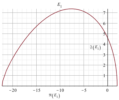
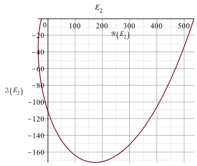
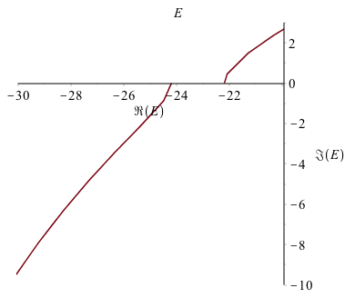
Figure 1. The orbit of $\varepsilon=\varepsilon_{1}(\sigma)$. Turning points (endpoints on the plot) are $\varepsilon_{1}(0)=1.9962511523$ and $\varepsilon_{1}(\sin\theta)=-22.1838257068$.

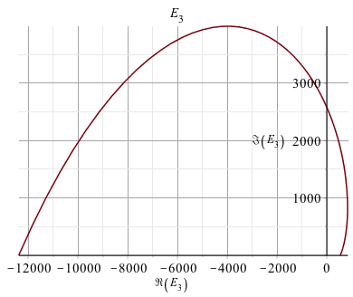
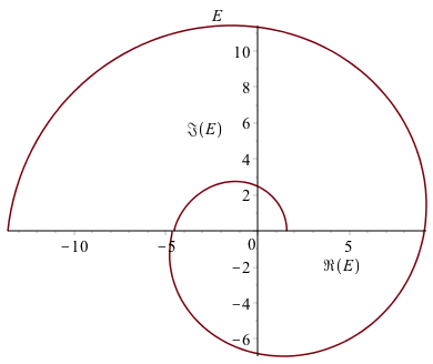
Figure 2. Left: the orbit of $\varepsilon=\varepsilon_{2}(\sigma)$. Turning points are $\varepsilon_{2}(0)=535.49351947$ and $\varepsilon_{2}(\sin\theta)=-24.183825694$. Right: the orbits of $\varepsilon_{1}(\sigma)$ and $\varepsilon_{2}(\sigma)$ in the vicinity of $\sigma=1/\sqrt{2}$. Recall that $\varepsilon_{1}(1/\sqrt{2})=-22.1838257068$ vs. $\varepsilon_{2}(1/\sqrt{2})=-24.183825694$.

Figure 3. Left: the orbit of $\varepsilon=\varepsilon_{3}(\sigma)$. Turning points are $\varepsilon_{3}(0)=535.49726832$ and $\varepsilon_{3}(\sin\theta)=-12391.6479693$. Right: Collection of $\varepsilon_{1}(\sigma)$, $\varepsilon_{2}(\sigma)$ and $\varepsilon_{3}(\sigma)$ in the logarithmic scale. Low resolution does not allow one to see the gaps between the orbits. Approximation of this spiral trajectory is $\varepsilon(\sigma)\simeq\operatorname{{e}}^{2\pi\mathsf{b}\sigma}$, $\sigma\geq 0$.

It is worth discussing the endpoints $\sigma=0$ and $\sigma=\sin\theta$ in general. The point $\sigma=0$ gives (see (119))

(129) $$W(1,\varepsilon)=\boldsymbol{\chi}(1,\varepsilon)\left(\boldsymbol{\chi}(q^{-2},\varepsilon)-q^{2}\boldsymbol{\chi}(q^{2},\varepsilon)\right)=0,$$

and the case

(130) $$\boldsymbol{\chi}(1,\varepsilon)=0$$

gives $\varepsilon_{k}(0)$ for even sheets,

(131) $$\begin{array}[]{l}\displaystyle\varepsilon_{2}(0)=\frac{1}{q^{2}}\left(1+q^{4}-q^{6}-q^{8}-q^{10}-2q^{12}-q^{14}+q^{18}+6q^{20}+11q^{22}+\dots\right),\\[11.38109pt] \displaystyle\varepsilon_{4}(0)=\frac{1}{q^{4}}\left(1+2q^{8}+q^{14}-q^{18}-3q^{20}-8q^{22}-13q^{24}+\dots\right),\\[11.38109pt] \displaystyle\varepsilon_{6}(0)=\frac{1}{q^{6}}\left(1+2q^{12}+q^{22}+q^{24}+q^{26}+2q^{32}+2q^{34}+\dots\right),\end{array}$$

and so on. Another branch

(132) $$\boldsymbol{\chi}(q^{-2},\varepsilon)-q^{2}\boldsymbol{\chi}(q^{2},\varepsilon)=0$$

gives $\varepsilon_{k}(0)$ for the odd sheets:

(133) $$\varepsilon_{1}(0)=2-2q^{2}-4q^{4}-2q^{6}+14q^{8}+50q^{10}+40q^{12}-268q^{14}-1136q^{16}+\dots,$$

(134) $$\varepsilon_{3}(0)=\frac{1}{q^{2}}(1+3q^{4}+3q^{6}+q^{8}-15q^{10}-52q^{12}-43q^{14}+264q^{16}+1127q^{18}+\dots),$$

and so on.

The point $\sigma=\sin\theta$ gives

(135) $$W(-q^{-1},\varepsilon)\sim\left(\boldsymbol{\chi}(-q^{-1},\varepsilon)-q\boldsymbol{\chi}(-q,\varepsilon)\right)\left(\boldsymbol{\chi}(-q^{-1},\varepsilon)+q\boldsymbol{\chi}(-q,\varepsilon)\right)$$

so that

(136) $$\boldsymbol{\chi}(-q^{-1},\varepsilon)-q\boldsymbol{\chi}(-q,\varepsilon)=0$$

gives the values for $\varepsilon_{k}(\sin\theta)$ on the odd sheets, for instance

(137) $$\varepsilon_{1}(\sin\theta)=-q^{-1}\left(1-q+q^{2}-q^{4}-q^{6}+q^{7}-2q^{8}+2q^{9}-2q^{10}+5q^{11}-4q^{12}+\dots\right).$$

Equation

(138) $$\boldsymbol{\chi}(-q^{-1},\varepsilon)+q\boldsymbol{\chi}(-q,\varepsilon)=0$$

gives the values for $\varepsilon_{k}(\sin\theta)$ on the even sheets, for instance

(139) $$\varepsilon_{2}(\sin\theta)=-q^{-1}\left(1+q+q^{2}-q^{4}-q^{6}-q^{7}-2q^{8}-2q^{9}-2q^{10}-5q^{11}-4q^{12}-\dots\right).$$

6.2. The spectrum

We turn now to the spectrum of the Hamiltonians (14).

The quantisation conditions (114) for real $\sigma$ are

(140) $$\textrm{Im}(G_{q}(s,\varepsilon))=0,\qquad\xi=-1,\quad\textrm{odd state,}$$

and

(141) $$\textrm{Re}(G_{q}(s,\varepsilon))=0,\qquad\xi=1,\quad\textrm{even state.}$$

One can see that formally there are two points $\sigma=0$ and $\sigma=\sin\theta$ on each sheet of the Riemann surface of $\varepsilon(\sigma)$ corresponding to these quantisation conditions. These are the exceptional cases as denominator $W(u)$ has the second order zeros while in the cases $\sigma=0$ for odd sheets, and $\sigma=\sin\theta$ for all sheets, the numerator of (106) has the first order zeros. Therefore, all these cases must be eliminated from the spectrum. On the other hand, if $\sigma=0$ on even sheets, corresponding to $\boldsymbol{\chi}(1)=0$, the numerator of (106) has second order zeros at some second order zeros of the denominator, but not at all of them and therefore the wave function (106) could not be a holomorphic function either. Theorem 5 concerns only the elimination of simple poles, and further analysis is needed to completely understand the situation with double poles.

6.2.1. Sheet 1.

Real and imaginary parts of $G_{q}(s,\varepsilon_{1}(\sigma))$ (the first sheet) are plotted in Fig. 4.

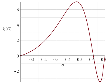
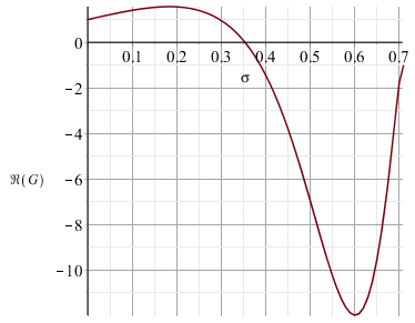
Figure 4. Left: $\Im(G_{q}(s,\varepsilon_{1}))$ as function of $\sigma$, $0\leq\sigma\leq\sin\theta$. Right: the same for $\Re(G_{q}(s,\varepsilon_{1}))$.

An even state from the first sheet is given by

(142) $$\sigma=\frac{1}{2}\sin\theta,\quad\varepsilon_{1}(\sigma)=4.59435880983691894\mathsf{i}.$$

This is the ground state.

An odd state from the first sheet is given by

(143) $$\sigma=0.6121173716461672675,\quad\varepsilon_{1}(\sigma)=-13.8783047780366906+6.161296243244348685\mathsf{i}.$$

The cases corresponding to $\sigma=0$ and $\sigma=\sin\theta$ are discarded.

6.2.2. Sheet 2.

Imaginary and real parts of the function $\displaystyle\frac{G_{q}(s,\varepsilon_{2}(\sigma))}{|G_{q}(s,\varepsilon_{2}(\sigma))|}$ (on the second sheet) are plotted in Fig. 5.

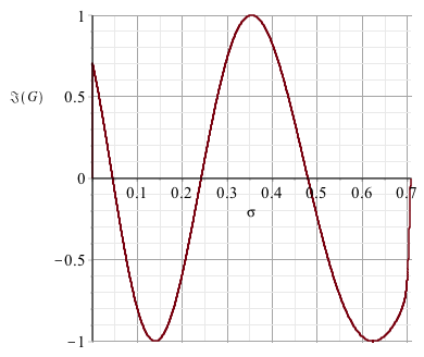
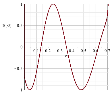
Figure 5. Left: $\displaystyle\frac{\Im(G_{q}(s,\varepsilon_{2}))}{|G_{q}(s,\varepsilon_{2})|}$ as function of $\sigma$, $0\leq\sigma\leq\sin\theta$. Right: the same for $\displaystyle\frac{\Re(G_{q}(s,\varepsilon))}{|G_{q}(s,\varepsilon_{2})|}$. Behaviour near $\sigma=0$ is misleading since one has an ambiguity $0/0$ there.

$$\begin{array}[]{|c|c|}\hline\cr\sigma&\varepsilon_{2}(\sigma)\\ \hline\cr 0.0449074054136668986&429.937612699070933-86.9352869839236228\mathsf{i}\\ 0.241612973133940861&87.33324987160330085-160.859744733070428\mathsf{i}\\ 0.478766031821187121&-33.7154767687408649-54.1710567496918622\mathsf{i}\\ \hline\cr\end{array}$$

Table 1. The odd states from the second sheet.

The odd and even states from the second sheet are given in Tables 1 and 2 respectively.

$$\begin{array}[]{|c|c|}\hline\cr\sigma&\varepsilon_{2}(\sigma)\\ \hline\cr 0.139460116715428804&234.614101715470239-167.345168305129794\mathsf{i}\\ \frac{1}{2}\sin\theta&-111.300184113096796\mathsf{i}\\ 0.623413635048467267&-31.32504489967260473-12.15333894226767358\mathsf{i}\\ \hline\cr\end{array}$$

Table 2. The even states from the second sheet.

The endpoint on the second orbit is given by

(144) $$\sigma=0,\quad\varepsilon_{2}(0)=535.493519473629469,$$

corresponding to $\boldsymbol{\chi}(1,\varepsilon_{2})=0$, but this value does not correspond to an eigenvalue since it is not possible to cancel all second order poles in the wave function.

6.3. Table of the spectrum for $\mathsf{b}=\operatorname{{e}}^{\mathsf{i}\pi/4}$

We summarize the spectrum from the first and second sheets in Tables 3 and 4 respectively. In our numerics we have used the precision $10^{-40}$, therefore all our digits for the energies are precise.

$$\begin{array}[]{|c|c|c|}\hline\cr\sigma&\text{parity}&\varepsilon_{1}(\sigma)\\ \hline\cr 0.35&\text{even}&4.59435880983691894\mathsf{i}\\ 0.61&\text{odd}&-13.8783047780366906+6.161296243244348685\mathsf{i}\\ \hline\cr\end{array}$$

Table 3. The states from the first sheet, $k=1$.

$$\begin{array}[]{|c|c|c|}\hline\cr\sigma&\text{parity}&\varepsilon_{2}(\sigma)\\ \hline\cr 0.62&\text{even}&-31.32504489967260473-12.15333894226767358\mathsf{i}\\ 0.48&\text{odd}&-33.7154767687408649-54.1710567496918622\mathsf{i}\\ 0.35&\text{even}&-111.300184113096796\mathsf{i}\\ 0.24&\text{odd}&87.33324987160330085-160.859744733070428\mathsf{i}\\ 0.14&\text{even}&234.614101715470239-167.345168305129794\mathsf{i}\\ 0.045&\text{odd}&429.937612699070933-86.9352869839236228\mathsf{i}\\ \hline\cr\end{array}$$

Table 4. The states from the second sheet, $k=2$.

7. The self-conjugate case $\hbar=2\pi$

Despite the fact that the special case $\mathsf{b}=1$ corresponds to the limiting value of the strong coupling regime $\theta\to 0$, we do not know how to approach that limit on the level of eigenvalues and eigenfunctions. For this reason, we treat that case separately, independently of the strong coupling regime. This case is very special as the operators $\boldsymbol{u}$ and $\boldsymbol{v}$ are positive self-adjoint and formally commuting, while both functional equations (16), (17) reduce to one and the same but still non-trivial functional difference equation

(145) $$\psi(x-\mathsf{i})+\psi(x+\mathsf{i})=(\varepsilon-2\cosh(2\pi x))\psi(x),$$

which, under the substitution

(146) $$\varphi(x):=\psi(\mathsf{i}x),$$

becomes an equation of the form

(147) $$\varphi(x-1)+\varphi(x+1)+(2\cos(2\pi x)-\varepsilon)\varphi(x)=0.$$

Despite being a special case of Harper’s functional equation [8] on the real line, this equation should nonetheless be considered on the entire complex plane as its quantum mechanical content is extracted from the restriction of its solutions to the imaginary axis.

7.1. The spectral curve

Due to periodicity of the potential, for any solution of (147), its Weil–Gel’fand–Zak transform [18, 6, 19]

(148) $$\tilde{\varphi}(x,y)=\sum_{m\in\mathbb{Z}}\varphi(x+m)\operatorname{{e}}^{-2\pi\mathsf{i}ym}$$

gives another solution which is quasi-periodic in $x$ and periodic in $y$:

(149) $$\tilde{\varphi}(x+1,y)=\operatorname{{e}}^{2\pi\mathsf{i}y}\tilde{\varphi}(x,y),\quad\tilde{\varphi}(x,y+1)=\tilde{\varphi}(x,y).$$

That means that the functional difference equation (147) is transformed into an algebraic functional equation

(150) $$\left(\cos(2\pi x)+\cos(2\pi y)-\frac{\varepsilon}{2}\right)\tilde{\varphi}(x,y)=0,$$

which means that the support of $\tilde{\varphi}(x,y)$ is localised to the spectral curve

(151) $$\Gamma_{\varepsilon}:=\left\{(x,y)\in\mathbb{C}^{2}\left|\ \cos(2\pi x)+\cos(2\pi y)=\frac{\varepsilon}{2}\right.\right\}$$

which covers the finite (affine) part of the elliptic curve

(152) $$\digamma_{\varepsilon}:=\left\{(u,v)\in\mathbb{C}^{2}\left|\ u+u^{-1}+v+v^{-1}=\varepsilon\right.\right\}$$

through the map

(153) $$\operatorname{q}\colon\Gamma_{\varepsilon}\to\digamma_{\varepsilon},\quad(x,y)\mapsto\left(\operatorname{{e}}^{2\pi\mathsf{i}x},\operatorname{{e}}^{2\pi\mathsf{i}y}\right).$$

Projection to the first component

(154) $$x\colon\Gamma_{\varepsilon}\to\mathbb{C}$$

is a covering map branched at the points satisfying the condition $\sin(2\pi y)=0$ which corresponds to a discrete infinite set of values of $x$:

(155) $$(-\mathsf{i}\alpha+\mathbb{Z})\cup(\mathsf{i}\alpha+\mathbb{Z})\cup(-\mathsf{i}\beta+\mathbb{Z})\cup(\mathsf{i}\beta+\mathbb{Z})$$

where parameters $\alpha=\alpha(\varepsilon)$ and $\beta=\beta(\varepsilon)$ are determined through the equations

(156) $$\varepsilon=2+2\cosh(2\pi\alpha)=4\cosh(\pi\alpha)^{2},$$

(157) $$\cosh(2\pi\beta)=\cosh(2\pi\alpha)+2\quad\Leftrightarrow\quad\sinh(\pi\beta)=\pm\cosh(\pi\alpha),$$

Since the spectrum of our operator is contained in $\mathbb{R}_{>4}$, we assume that $\varepsilon\in\mathbb{R}_{>4}$. In that case, we can choose $\alpha$ and $\beta$ in a canonical way as real positive solutions of equations (156) and (157).

The automorphism group of the spectral curve $\Gamma_{\varepsilon}$ contains a subgroup generated by three elements

(158) $$\rho,\sigma,\tau\colon\Gamma_{\varepsilon}\to\Gamma_{\varepsilon},\quad\rho(x,y)=(-x,y),\quad\sigma(x,y)=(y,x),\quad\tau(x,y)=(x+1,y).$$

The two involutions $\rho$ and $\sigma$ cover involutions $\dot{\rho}$ and $\dot{\sigma}$ of $\digamma_{\varepsilon}$, while $\tau$ acts fiber-wise, i.e.

(159) $$\operatorname{q}\circ\rho=\dot{\rho}\circ\operatorname{q},\quad\operatorname{q}\circ\sigma=\dot{\sigma}\circ\operatorname{q},\quad\operatorname{q}\circ\tau=\operatorname{q}.$$

7.2. The deformed symplectic potential

For the construction of a Bloch–Jost function to be defined below, we will use the restrictions to $\Gamma_{\varepsilon}$ of a one parameter family of deformed (holomorphic) symplectic potentials on $\mathbb{C}^{2}$

(160) $$\theta_{\lambda}:=\left(x+\frac{\lambda}{\sin(2\pi x)}\right)\operatorname{d}\!y,\quad\lambda\in\mathbb{C},$$

where the non-deformed part

(161) $$\theta_{0}=x\operatorname{d}\!y$$

is the restriction of the standard holomorphic symplectic potential in $\mathbb{C}^{2}$, while the deforming part is given by the pull-back of a holomorphic 1-form on $\digamma_{\varepsilon}$

(162) $$\frac{\operatorname{d}\!y}{\sin(2\pi x)}=-\frac{\operatorname{d}\!x}{\sin(2\pi y)}=\operatorname{q}^{*}(\omega),\quad\omega=\frac{\operatorname{d}\!v}{\pi v(u-u^{-1})}=-\frac{\operatorname{d}\!u}{\pi u(v-v^{-1})},$$

which is unique up to multiplication by a non-zero complex constant. With respect to the automorphisms (158), the form $\theta_{\lambda}$ has the following properties:

(163) $$\rho^{*}(\theta_{\lambda})=-\theta_{\lambda},\quad\sigma^{*}(\theta_{\lambda})=\operatorname{d}(xy)-\theta_{\lambda},\quad\tau^{*}(\theta_{\lambda})=\operatorname{d}\!y+\theta_{\lambda}.$$

7.3. The Bloch–Jost function

Definition 1.

A holomorphic function $f\colon\Gamma_{\varepsilon}\to\mathbb{C}$ is called Bloch–Jost function if it satisfies the functional relations

(164) $$f(x+1,y)\operatorname{{e}}^{-2\pi\mathsf{i}y}=f(x,y+1)=f(x,y),\quad\forall(x,y)\in\Gamma_{\varepsilon}.$$

For a fixed base point $P_{0}\in\Gamma_{\epsilon}$, let $\operatorname{p}\colon\tilde{\Gamma}_{\varepsilon}\to\Gamma_{\varepsilon}$ be the universal covering given by the homotopy classes of all paths starting from $P_{0}$. We define

(165) $$g_{\lambda,\varepsilon}\colon\tilde{\Gamma}_{\varepsilon}\to\mathbb{C}_{\neq 0},\quad\gamma\mapsto\operatorname{{e}}^{2\pi\mathsf{i}\int_{\gamma}\theta_{\lambda}}$$

Theorem 6.

Let $(\lambda,\varepsilon)\in\mathbb{C}\times\mathbb{R}_{>4}$ be such that

(166) $$g_{\lambda,\varepsilon}(\gamma)=1,$$

for any $\gamma$ for which $x\circ\gamma$ and $\operatorname{q}\circ\gamma$ are closed paths. Then, there exists a Bloch–Jost function $f$ such that $g_{\lambda,\varepsilon}=\operatorname{p}^{*}(f)$.

Proof.

The fact that $g_{\lambda,\varepsilon}=\operatorname{p}^{*}(f)$ for some $f\colon\Gamma_{\varepsilon}\to\mathbb{C}$ is immediate. It suffices to remark that any closed path on $\Gamma_{\varepsilon}$ projects down to closed paths both in $\mathbb{C}$ and $\digamma_{\varepsilon}$. So, we need to verify only the quasi-periodicity properties of $f$.

Let paths $\mu,\nu\colon[0,1]\to\Gamma_{\varepsilon}$ be such that

(167) $$\mu(0)=P_{0},\quad\mu(1)=\nu(0)=(x,y),\quad\nu(1)=(x,y+1).$$

Then, we have

(168) $$f(x,y+1)=\operatorname{{e}}^{2\pi\mathsf{i}\int_{\mu\cdot\nu}\theta_{\lambda}}=\operatorname{{e}}^{2\pi\mathsf{i}\int_{\mu}\theta_{\lambda}}\operatorname{{e}}^{2\pi\mathsf{i}\int_{\nu}\theta_{\lambda}}=f(x,y),$$

since both $x\circ\nu$ and $\operatorname{q}\circ\nu$ are closed.

Redefine now $\mu,\nu\colon[0,1]\to\Gamma_{\varepsilon}$ so that

(169) $$\mu(0)=P_{0},\quad\mu(1)=\nu(0)=(x,y),\quad\nu(1)=(x+1,y).$$

Then, we have

(170) $$f(x+1,y)=\operatorname{{e}}^{2\pi\mathsf{i}\int_{\mu\cdot\nu}\theta_{\lambda}}=\operatorname{{e}}^{2\pi\mathsf{i}\int_{\mu}\theta_{\lambda}}\operatorname{{e}}^{2\pi\mathsf{i}\int_{\nu}\theta_{\lambda}}=f(x,y)\operatorname{{e}}^{2\pi\mathsf{i}\int_{\nu}\theta_{\lambda}},$$

where, this time, the path $x\circ\nu$ is not closed. Using the secon equality in (163), we have

(171) $$\operatorname{{e}}^{2\pi\mathsf{i}\int_{\nu}\theta_{\lambda}}=\operatorname{{e}}^{2\pi\mathsf{i}\int_{\sigma\circ\nu}\sigma^{*}\theta_{\lambda}}=\operatorname{{e}}^{2\pi\mathsf{i}\int_{\sigma\circ\nu}\operatorname{d}(xy)}\operatorname{{e}}^{-2\pi\mathsf{i}\int_{\sigma\circ\nu}\theta_{\lambda}}=\operatorname{{e}}^{2\pi\mathsf{i}y}$$

where we have used the fact that the paths $x\circ\sigma\circ\nu$ and $\operatorname{q}\circ\sigma\circ\nu$ are closed. ∎

7.4. The spectral equations

We call equations (166) spectral equations. Our goal here is to reduce them to a minimal set so that any other equation is a consequence of the equations from that minimal set. By using two functions

(172) $$r\colon\mathbb{R}\to[\alpha,\beta],\quad\cosh(2\pi r(t))=1-\cos(\pi t)+\cosh(2\pi\alpha),$$

and

(173) $$s\colon\mathbb{R}\to[0,\alpha],\quad\sinh(\pi s(t))=\sinh(\pi\alpha)\sin(\pi t),$$

we define four paths $\xi,\check{\xi},\zeta,\hat{\zeta}\colon[0,1]\to\Gamma_{\varepsilon}$ by

(174) $$\xi(t)=(\mathsf{i}s(t+1/2),\mathsf{i}s(t)),\quad\check{\xi}(t)=(-\mathsf{i}s(t+1/2),-\mathsf{i}s(t)).$$

and

(175) $$\zeta(t)=(\mathsf{i}r(t),t/2),\quad\hat{\zeta}(t)=(\mathsf{i}r(1-t),(t+1)/2).$$

We observe that $(\xi,\check{\xi})$ and $(\zeta,\hat{\zeta})$ are composable pairs, $\xi\cdot\check{\xi}$ being closed, while $\zeta\cdot\hat{\zeta}$ projects down to closed paths both in $\mathbb{C}$ and $\digamma_{\varepsilon}$. Moreover, their images generate the fundamental group of $\digamma_{\varepsilon}$, which means that the equations

(176) $$\operatorname{{e}}^{2\pi\mathsf{i}\int_{\xi\cdot\check{\xi}}\theta_{\lambda}}=\operatorname{{e}}^{2\pi\mathsf{i}\int_{\zeta\cdot\hat{\zeta}}\theta_{\lambda}}=1$$

constitute a complete set of spectral equations. We calculate

(177) $$\int_{\xi\cdot\check{\xi}}\theta_{\lambda}=2\int_{\xi}\theta_{\lambda}=4\int_{0}^{1/2}\left(\frac{\lambda}{\sinh(2\pi s(t+1/2))}-s(t+1/2)\right)s^{\prime}(t)\operatorname{d}\!t=:A\lambda-\tilde{A}$$

and

(178) $$\int_{\zeta\cdot\hat{\zeta}}\theta_{\lambda}=2\int_{\zeta}\theta_{\lambda}=\mathsf{i}\int_{0}^{1}\left(r(t)-\frac{\lambda}{\sinh(2\pi r(t))}\right)\operatorname{d}\!t=:\mathsf{i}(\tilde{B}-\lambda B)$$

where $A,\tilde{A},B,\tilde{B}$ are positive functions of $\varepsilon$ satisfying the inequality

(179) $$A\tilde{B}-B\tilde{A}>0$$

which is seen if we write out all integrals explicitly:

(180) $$A\tilde{B}-B\tilde{A}=4\int_{[0,1/2]\times[0,1]}\operatorname{d}(t,u)\frac{s^{\prime}(t)\left(r(u)\sinh(2\pi r(u))-s(t+1/2)\sinh(2\pi s(t+1/2))\right)}{\sinh(2\pi s(t+1/2))\sinh(2\pi r(u))}$$

and take into account the inequalities

(181) $$0\leq s(t)\leq\alpha\leq r(u)\leq\beta,\quad\forall t,u\in\mathbb{R}.$$

Now, the spectral equations (176) imply that

(182) $$A\lambda-\tilde{A}=:n+1\in\mathbb{Z},\quad\mathsf{i}(\tilde{B}-\lambda B)\in\mathbb{Z},$$

so that the second condition fixes a unique choice for $\lambda$,

(183) $$\lambda=\tilde{B}/B,$$

while the first condition becomes a quantisation condition for the energy:

(184) $$A\tilde{B}-B\tilde{A}=(n+1)B,\quad n\in\mathbb{Z}_{\geq 0},$$

where we have taken into account the inequality (179).

Numerical calculation at $n=0$ for the ground state energy $\varepsilon_{0}$ gives the result

(185) $$\log(\varepsilon_{0})=2.88181542992629678247713987172363292221616219\dots$$

which is in agreement with formula (5.39) of [7].

7.5. The eigenfunctions

Theorem 7.

Let $(\lambda,\varepsilon)\in\mathbb{C}\times\mathbb{R}_{>4}$ satisfy the assumptions of Theorem 6, and choose the base point $P_{0}=(\mathsf{i}\alpha,0)\in\Gamma_{\varepsilon}$. Then, there exists a holomorphic function $\varphi\colon\mathbb{C}\to\mathbb{C}$ such that

(186) $$\sin(2\pi y)\varphi(x)=\sin\left(2\pi\int_{\gamma}\theta_{\lambda}\right),\quad\forall(x,y)\in\Gamma_{\varepsilon},$$

for any path $\gamma\colon[0,1]\to\Gamma_{\varepsilon}$ such that $\gamma(0)=P_{0}$ and $\gamma(1)=(x,y)$. In particular, $\varphi(x)$ is a solution of the functional difference equation (147).

Proof.

The right hand side of (186) can be rewitten in the form

(187) $$2\mathsf{i}\sin\left(2\pi\int_{\gamma}\theta_{\lambda}\right)=f(x,y)-f(x,-y),$$

where $f(x,y)$ is the Bloch–Jost function defined by

(188) $$f(x,y):=\operatorname{{e}}^{2\pi\mathsf{i}\int_{\gamma}\theta_{\lambda}}$$

and the choice of the base point is such that

(189) $$f(x,y)f(x,-y)=1.$$

Thus, the function

(190) $$h(x,y):=\frac{f(x,y)-f(x,-y)}{\sin(2\pi y)}$$

is explicitly periodic and symmetric in $y$:

(191) $$h(x,y+1)=h(x,y)=h(x,-y)$$

On the other hand, if $(a,b)\in\Gamma_{\varepsilon}$ then

(192) $$x^{-1}(a)=\{a\}\times(\{b+\mathbb{Z}\}\cup\{-b+\mathbb{Z}\})$$

so that

(193) $$h(a,b^{\prime})=h(a,b),\quad\forall(a,b^{\prime})\in x^{-1}(a),$$

i.e. there exists a function $\varphi\colon\mathbb{C}\to\mathbb{C}$ such that $h=x^{*}(\varphi)$. It remains to see that $\varphi(x)$ is holomorphic at any of the ramification points (155) corresponding to $\sin(2\pi y)=0$, i.e. either $y=0$ or $y=1/2$. The case $y=0$ is explicitly regular. To see the regularity at $y=1/2$, it suffices to see that

(194) $$f(\pm\mathsf{i}\beta,1/2)^{2}=1.$$

In the case of plus sign, from the definition (175), it follows that

(195) $$f(\mathsf{i}\beta,1/2)=\operatorname{{e}}^{2\pi\mathsf{i}\int_{\zeta}\theta_{\lambda}}=1$$

where the last equality is satisfied due to (177) and (183).

In the case of minus sign in (194), we verify it by using (195) and the symmetry property of the Bloch–Jost function under the negation of the first component:

(196) $$f(-x,y)=f(-\mathsf{i}\alpha,0)/f(x,y)=\operatorname{{e}}^{2\pi\mathsf{i}\int_{\xi}\theta_{\lambda}}/f(x,y)=(-1)^{n+1}/f(x,y)$$

where we have used definition (174) and the equation in the first part of (182). ∎

Thus, we have solved the spectral problem (145), where the spectrum is determined by equations (182) and the corresponding eigenfunctions are given by the formula $\psi(x)=\varphi(\mathsf{i}x)$ for all $x\in\mathbb{R}$, where $\varphi(x)$ is defined in (186). These eigenfunctions coincide with the ones constructed in [15].

References

- [1] Mina Aganagic, Robbert Dijkgraaf, Albrecht Klemm, Marcos Mariño, and Cumrun Vafa. Topological strings and integrable hierarchies. Comm. Math. Phys., 261(2):451–516, 2006.
- [2] Rodney J. Baxter. Exactly solved models in statistical mechanics. Academic Press, Inc. [Harcourt Brace Jovanovich, Publishers], London, 1982.
- [3] Vladimir V. Bazhanov, Sergei L. Lukyanov, and Alexander B. Zamolodchikov. Spectral determinants for Schrödinger equation and -operators of conformal field theory. In Proceedings of the Baxter Revolution in Mathematical Physics (Canberra, 2000), volume 102, pages 567–576, 2001.
- [4] Patrick Dorey and Roberto Tateo. Anharmonic oscillators, the thermodynamic Bethe ansatz and nonlinear integral equations. J. Phys. A, 32(38):L419–L425, 1999.
- [5] L. D. Faddeev. Discrete Heisenberg–Weyl group and modular group. Lett. Math. Phys., 34(3):249–254, 1995.
- [6] I. M. Gel′fand. Expansion in characteristic functions of an equation with periodic coefficients. Doklady Akad. Nauk SSSR (N.S.), 73:1117–1120, 1950.
- [7] Alba Grassi, Yasuyuki Hatsuda, and Marcos Mariño. Topological strings from quantum mechanics. Ann. Henri Poincaré, 17(11):3177–3235, 2016.
- [8] P. G. Harper. Single band motion of conduction electrons in a uniform magnetic field. Proc. Phys. Soc. A, 68(10):874–892, 1955.
- [9] Yasuyuki Hatsuda, Hosho Katsura, and Yuji Tachikawa. Hofstadter’s butterfly in quantum geometry. arXiv:1606.01894, 2016.
- [10] Yasuyuki Hatsuda, Yuji Sugimoto, and Zhaojie Xu. Calabi–Yau geometry meets electrons in 2d. arXiv:1701.01561, 2017.
- [11] Rinat Kashaev and Marcos Mariño. Operators from Mirror Curves and the Quantum Dilogarithm. Comm. Math. Phys., 346(3):967–994, 2016.
- [12] Rinat Kashaev, Marcos Mariño, and Szabolcs Zakany. Matrix Models from Operators and Topological Strings, 2. Ann. Henri Poincaré, 17(10):2741–2781, 2016.
- [13] Amir-Kian Kashani-Poor. Quantization condition from exact WKB for difference equations. arXiv:1604.01690, 2016.
- [14] Marcos Mariño. Spectral theory and mirror symmetry. arXiv:1506.07757, 2015.
- [15] Marcos Mariño and Szabolcs Zakany. Exact eigenfunctions and the open topological string. arXiv:1606.05297, 2016.
- [16] Nikita A. Nekrasov and Samson L. Shatashvili. Quantization of integrable systems and four dimensional gauge theories. In XVIth International Congress on Mathematical Physics, pages 265–289. World Sci. Publ., Hackensack, NJ, 2010.
- [17] S. M. Sergeev. A quantization scheme for modular -difference equations. Teoret. Mat. Fiz., 142(3):500–509, 2005.
- [18] André Weil. L’intégration dans les groupes topologiques et ses applications. Actual. Sci. Ind., no. 869. Hermann et Cie., Paris, 1940. [This book has been republished by the author at Princeton, N. J., 1941.].
- [19] J. Zak. Finite translations in solid state physics. Phys. Rev. Lett., 19:1385–1397, 1967.