Globally Optimal Beamforming Design for Downlink CoMP transmission with Limited Backhaul Capacity

Abstract

This paper considers a multicell downlink channel in which multiple base stations (BSs) cooperatively serve users by jointly precoding shared data transported from a central processor over limited-capacity backhaul links. We jointly design the beamformers and BS-user link selection so as to maximize the sum rate subject to user-specific signal-to-interference-noise (SINR) requirements, per-BS backhaul capacity and per-BS power constraints. As existing solutions for the considered problem are suboptimal and their optimality remains unknown due to the lack of globally optimal solutions, we characterized this gap by proposing a globally optimal algorithm for the problem of interest. Specifically, the proposed method is customized from a generic framework of a branch and bound algorithm applied to discrete monotonic optimization. We show that the proposed algorithm converges after a finite number of iterations, and can serve as a benchmark for existing suboptimal solutions and those that will be developed for similar contexts in the future. In this regard, we numerically compare the proposed optimal solution to a current state-of-the-art, which show that this suboptimal method only attains 70% to 90% of the optimal performance.

Index Terms—  Multicell cooperation, limited backhaul, sum rate maximization, discrete monotonic optimization.

1 Introduction

Due to the explosive growth of wireless devices and data services, increasing network capacity has become a critical target for the current and future wireless networks. As well concluded from pioneer research, intercell-inteference is a key factor limiting the overall spectral efficiency offered by wireless technologies [1]. Schemes turning interference from nuisance to the users’ benefit, such as cooperative multipoint (CoMP) processing has been proposed [2]. The central idea is to allow for joint processing by multiple transmitters, thereby turning the interference to useful signals [1, 2, 3]. The two main forms of CoMP processing are interference coordination and data sharing. In the latter, data for a specific is transmitted from multiple base stations (BSs), which is the focus of this paper.

The promise of multicell BS cooperation is often seen under the assumption that the backhaul network is able to deliver an enormous signaling overhead from a central processor (CP) to all BSs. In practice, the capacity of the backhaul communications is limited, especially, with wireless backhauling [4]. Therefore, a number of recent research efforts have investigated solutions to optimize various performance measures in finite-capacity backhaul networks for different system models. Those include, e.g., sum rate maximization [5], joint backhaul and power minimization [6], energy efficiency maximization [7], and backhaul usage minimization [8]. To deal with the backhaul constraint in particular, the aforementioned works have adopted a BS-user link selection scheme where each BS in the network transmits data to only a proper subset of users in order to reduce the backhaul consumed.

This paper is to explore the optimal performance of maximizing the sum rate of cooperative multicell downlink under limited backhaul capacity constraints. In particular, we propose a beamforming design to maximize the achievable sum rate while satisfying per-BS backhaul capacity, per-BS power constraints, and user-specific signal-to-interference-noise (SINR) requirements. The latter condition ensures the minimum quality of service for each user regardless of the user’s location in a cell. To cope with the backhaul limitation, a BS-user link selection scheme is necessary and will be studied in this paper. Thus, the resulting problem is in fact a joint beamforming and BS-user link selection design which naturally leads to a mixed-Boolean non-convex program (MBNP), which is generally known to be NP-hard and optimal solutions are hard to derive. A suboptimal solution based on reweighted $l_{1}$-norm was proposed for a similar problem in the considered context [5]. Although this approach yields solutions with reasonably low complexity, its achieved performance in relation to the optimal one has not been investigated yet. To fill this gap, we propose an algorithm that achieves a global optimum of the design problem. The proposed method is based on a discrete monotonic optimization (DMO) framework which is difficult to connect to the original problem formulation. In particular, the hidden monotonicity of the considered problem is exposed by a novel proposed transformation. This then facilitates an efficient customization of a discrete brach-reduce-and-bound (DBRB) method to find a global optimum. Numerical results are provided to demonstrate the convergence of the proposed optimal algorithm and the performance gains over known methods.

2 System Model and Problem Formulation

Consider a multiple-input single-output (MISO) downlink transmission of wireless systems where there are $B$ multiple-antenna BSs, each is equipped with $M$ antennas, jointly serving $K$ single-antenna users. Suppose that all BSs in the network are connected to a CP through backhaul links of limited capacity. We also assume that the CP has the data of all users and perfectly knows the associated channel state information (CSI) and the necessary control information. The data symbol for user $k$ is denoted by $d_{k}$, assumed to have unit energy, i.e., $\mathbb{E}[|d_{k}|^{2}]=1$. Herein, we adopt linear precoding, i.e., $d_{k}$ is multiplied with beamformer ${\bf w}_{b,k}\in\mathbb{C}^{M\times 1}$ before being transmitted by BS $b$. Accordingly, under flat fading channels, the received signal ${\bf y}_{k}\in\mathbb{C}^{M\times 1}$ of user $k$ can be written as

$${\bf y}_{k}={\textstyle\sum_{b=1}^{B}}{\bf h}_{b,k}{\bf w}_{b,k}d_{k}+{\textstyle\sum_{b=1}^{B}\sum_{j\neq k}^{K}}\mathbf{h}_{b,k}\mathbf{w}_{b,j}d_{j}+\sigma_{k},$$ (1)

where ${\bf h}_{b,k}\in\mathbb{C}^{1\times M}$ is the (row) vector representing the channel of $(b,k)$, and $\sigma_{k}\sim\mathcal{CN}(0,N_{0})$ is the additive white Gaussian noise at user $k$. For notational simplicity, let ${\bf h}_{k}\triangleq[{\bf h}_{1,k},{\bf h}_{2,k},\ldots,{\bf h}_{B,k}]\in\mathbb{C}^{1\times MB}$ and ${\bf w}_{k}\triangleq[{\bf w}_{1,k}^{T},{\bf w}_{2,k}^{T},\ldots,{\bf w}_{B,k}^{T}]^{T}$ $\in\mathbb{C}^{MB\times 1}$ be the aggregate vectors of all channels and beamformers from all BSs to user $k$, respectively. We also denote by ${\bf w}$ the beamforming vector encompassing all ${\bf w}_{k}$. We further assume that single-user decoding is performed. In this regard, the intercell-interference is treated as Gaussian noise, and thus the SINR at user $k$ can be written as

$$\gamma_{k}({\bf w})\triangleq|{\bf h}_{k}{\bf w}_{k}|^{2}({\textstyle\sum_{j=1,j\neq k}^{K}}|{\bf h}_{k}{\bf w}_{j}|^{2}+WN_{0})^{-1}.$$ (2)

The data rate of user $k$ is given by $R_{k}({\bf w})\triangleq W\log(1+\gamma_{k}({\bf w}))$, where $W$ is the bandwidth. To simplify the notation, we will drop $W$ in the sequel.

Let us denote by $x_{b,k}\in\{0,1\}$ the selection preference variable where $x_{b,k}=1$ indicates that transmission link between BS $b$ and user $k$ is active and $x_{b,k}=0$ otherwise. The backhaul usage of BS $b$ is the sum of data streams of its served users given by $C_{b}^{\text{BH}}\triangleq{\textstyle\sum_{k=1}^{K}}x_{b,k}R_{k}({\bf w})$ which is upper bounded by a link capacity $\bar{C}$, i.e., $C_{b}^{BH}\leq\bar{C}$. To reduce the backhaul usage, BS $b$ can turn off transmissions to some users. That is, the CP does not deliver those users’ information to BS $b$. Also, beamformers associated to inactive transmissions are forced to be zero, i.e., ${\bf w}_{b,k}=0$ if $x_{b,k}=0$. To capture this relation, we introduce the constraint $\|{\bf w}_{b,k}\|\leq x_{b,k}u_{b,k}$ where $u_{b,k}$ represents a soft power level of ${\bf w}_{b,k}$ and will be optimized under the considered power constraint.

Based on the above discussions, the problem of joint beamforming design and BS-user link selection which maximizes the sum rate subject to user-specific SINR requirements, per-BS backhaul capacity and power constraints can be formulated as

$$\underset{{\bf w},{\bf x},{\bf u}}{\text{maximize}} \ \ \ {\textstyle\sum_{k=1}^{K}}R_{k}({\bf w})$$ (3a)

subject to $$\ \ \ {\textstyle\sum_{k=1}^{K}}x_{b,k}R_{k}({\bf w})\leq\bar{C},\ \forall b,k$$ (3b)

$$\ \ \ \gamma_{k}({\bf w})\geq\bar{\gamma}_{0},\forall k$$ (3c)

$$\ \ \ \|{\bf w}_{b,k}\|_{2}^{2}\leq x_{b,k}u_{b,k},\ \forall b,k$$ (3d)

$$\ \ \ {\textstyle\sum_{k=1}^{K}}u_{b,k}\leq\bar{P},\ \forall b,k$$ (3e)

$$\ \ \ {\textstyle\sum_{b=1}^{B}}x_{b,k}\geq 1,\ \forall b,k$$ (3f)

$$\ \ \ x_{b,k}\in\{0,\ 1\},\ \forall b,k,$$ (3g)

where $\bar{\gamma}_{0}$ is the per-user targeted SINR, and $\bar{P}$ is the per-BS transmit power budget. We also denoted ${\bf x}\triangleq[x_{1,k},\ldots x_{b,k},\ldots,x_{B,K}]^{T}\in\{0,1\}^{BK}$ and ${\bf u}\triangleq[u_{1,k},\ldots u_{b,k},\ldots,u_{B,K}]^{T}\in\mathbb{R}_{+}^{BK}$ . Herein (3f) is added to ensure each user is always served by at least one BS. Note that user-specific SINR constraint (3c) can be represented as an SOC constraint following the results in [9] as

$$\mathbf{h}_{k}\mathbf{w}_{k}\geq\sqrt{\bar{\gamma}_{0}({\textstyle\sum_{j\neq k}^{K}}|\mathbf{h}_{k}\mathbf{w}_{j}|^{2}+WN_{0})}\ ,\ \Im(\mathbf{h}_{k}\mathbf{w}_{k})=0.$$ (4)

It is now clear that problem (3) belongs to the class of MBNP due to the Boolean variable ${\bf x}$, the nonconvex objective (3a) and the nonconvex constraint (3b). Recall that a suboptimal solution for this problem was proposed in [5] using a sparsity inducing norm approach. Thus, there is a need to understand its achieved performance, and to see if there is a room for improvement.

3 Proposed Optimal Solution

We derive an algorithm which globally solves (3) by customizing a state-of-the-art global discrete optimization technique namely discrete monotonic optimization. This framework has been applied to find a global optimum of different MBNP problems in wireless communications [10, 11, 12]. It is worth noting that although continuous monotonic optimization (MO) [13] can also handle discrete constraints in (3g) by writing $x_{bk}\in\{0,1\}\Leftrightarrow x_{b,k}^{2}-x_{bk}\geq 0,\ x_{b,k}\in[0,1]$. However it potentially returns only approximate solutions by a finite number of iterations. Thus, DMO has been developed in [14] to compute exact optimal solutions. In this section, we will adapt the discrete branch-reduce-and-bound strategy in DMO, to solve the design problem (3). Before proceeding further, we remark that basic concepts of the MO such as increasing function, normal cone and box are used throughout the rest of this section. Their definitions can be found in [13] and are omitted in this paper due to space limitation.

The current formulation of the design problem is not amendable for a direct application of the DBRB since (3) does not hold the monotonicity property w.r.t. the involved variables. Thus, a further proper translation is required. For this purpose, let us introduce new slack variable $z_{k}$ and rewrite (3) as

$$\underset{{\bf w},{\bf x},{\bf u},{\bf z}}{\text{maximize}} \ \ \ {\textstyle\sum_{k=1}^{K}}z_{k}$$ (5a)

subject to $$\ \ \mathbf{h}_{k}\mathbf{w}_{k}\geq\sqrt{(e^{z_{k}}-1)({\textstyle\sum_{j\neq k}^{K}}|\mathbf{h}_{k}\mathbf{w}_{j}|^{2}+WN_{0})}$$ (5b)

$$\ \ \ {\textstyle\sum_{k=1}^{K}}x_{b,k}z_{k}\leq\bar{C}$$ (5c)

$$\ \ \ \eqref{eq:soft power},\eqref{eq:power},\eqref{eq:min:connectivity},\eqref{eq:boolean},\eqref{eq:QoS:SoCP},\vspace{-3mm}$$ (5d)

where ${\bf z}\triangleq[z_{1},\ldots,z_{K}]^{T}$. The equivalence between (3) and (5) can be verified as (5b) holds with equality at the optimum. Now we can observe that a better objective of (5) is always achieved if we keep increasing each of $z_{k}$ as long as it is still in the feasible set of (5). In addition, the feasibility of ${\bf z}$ is established depending on ${\bf x}$ as can be seen in (5c). Furthermore, constraint (5c) is monotone w.r.t. ${\bf z}$ and ${\bf x}$. These three observations imply that (5) is suitable for a direct application of the DBRB to find the optimal solutions of ${\bf z}$ and ${\bf x}$. Before describing the details, we introduce new notations for the ease of exposition. Let ${\bf s}=[{\bf x}^{T},{\bf z}^{T}]^{T}\in\mathbb{R}_{+}^{N_{x}+N_{z}}$ be the variable vector of interest where $N_{x}=BK$ and $N_{z}=K$ are dimensions of the Boolean and continuous vectors ${\bf x}$ and ${\bf z}$, respectively. Let ${\cal S}$ be the feasible set of problem (5), i.e., $\begin{aligned} {\cal S}=\{{\bf s}\in\mathbb{R}_{+}^{N}\ |&\ \eqref{eq:soft power},\eqref{eq:power},\eqref{eq:min:connectivity},\eqref{eq:boolean},\eqref{eq:QoS:SoCP},\eqref{eq:rate:epi},\eqref{eq:BH:reform}\}\end{aligned}$ where $N=N_{x}+N_{z}$ and ${\cal S}$ is normal and finite since it is upper bounded by the power and backhaul constraints. Additionally, the feasible set ${\cal S}$ is contained in a box $D=[{\bf a},{\bf b}]\in\mathbb{R}_{+}^{N}$ whose vertices are determined as follows. It is easily seen that $a_{i}=0$ and $b_{i}=1$ for $i=1,\ldots N_{x}$ since $x_{b,k}\in\{\underline{x}_{b,k},\overline{x}_{b,k}\}=\{0,1\}$. On the other hand, variable $z_{k}$ is bounded below by $z_{k}\geq\underline{z}_{k}=\log(1+\bar{\gamma}_{0})$. In addition, we can verify $z_{k}\leq\overline{z}_{k}=\min\{B\bar{C},\log(1+|{\bf h}_{k}{\bf w}_{k}|^{2}/WN_{0})\}\leq\min\{B\bar{C},\log(1+\|{\bf h}_{k}\|_{2}^{2}\|{\bf w}_{k}\|_{2}^{2}/WN_{0})\}\leq\min\{B\bar{C},\log(1+B\bar{P}\|{\bf h}_{k}\|_{2}^{2}/WN_{0})\}$. That is to say, for $i=N_{x}+1,\ldots,N$, we have $a_{i}=\log(1+\bar{\gamma}_{0})$ and $b_{i}=\min\{B\bar{C},\ \log(1+B\bar{P}\|{\bf h}_{k}\|_{2}^{2}/WN_{0})\}$ where $k=i-N_{x}$. To sum up, the lower and upper vertices of box $D$ are given by

$${\bf a}=[{\bf 0}_{N_{x}},\ \log(1+\bar{\gamma}_{0})\times{\bf 1}_{N_{z}}]$$

$${\bf b}=[{\bf 1}_{N_{x}},\ \left\{\min\{B\bar{C},\ \log(1+B\bar{P}\|{\bf h}_{k}\|_{2}^{2}/WN_{0})\}\right\}_{k=1}^{N_{z}}],\vspace{-3mm}$$

where ${\bf 0}_{N_{x}}$, $\bm{1}_{N_{x}}$ and ${\bf 1}_{N_{z}}$ denote vectors of all zero and one values of the size given in the subscripts, respectively. At this line, problem (5) can be compactly rewritten as

$$\max\{f({\bf s})\triangleq{\textstyle\sum_{i=N_{x}+1}^{N}}s_{i}\ |\ {\bf s}\in{\cal S}\subset D\}.\vspace{-2mm}$$ (6)

We are now ready to describe the DBRB algorithm to solve (6) optimally. Generally, this method is an iterative procedure consisting of three basic operations at each iteration: branching, reduction, and bounding. More specifically, starting from the box $[{\bf a},{\bf b}]$, we iteratively divide it into smaller and smaller ones, remove boxes that do not contain an optimal solution, search over remaining boxes for a better optimal solution until fulfilling the stopping criterion. Different to the continuous procedure, to guarantee the exact solution of the Boolean variable, $N_{x}$ first elements on the cutting plane of boxes are adjusted to be dropped in the Boolean set during the branching and reduction operations. The adjustment rule is motivated by the monotonicity property to ensure not cutting off any feasible solution [14]. The algorithm terminates when the size of boxes containing the optimal solution is small enough. DBRB algorithm is described in Alg. 1 where details are given as follows. For notational convenience, we denote by $\vartheta_{n}$, ${\cal R}_{n}$, $f_{U}(V)$ and $f_{L}(V)$ the current best objective (cbo), the set of boxes containing an optimal solution at iteration $n$, the upper bound and lower bound value of $f({\bf s})$ over box $V$, respectively.

Branching

We start iteration $n$ by selecting a box in ${\cal R}_{n}$ and splitting it into two smaller ones. A candidate box $V_{c}\in{\cal R}_{n}$ for branching is picked up by the improving bound rule [13], i.e., $V_{\text{c}}=\arg\max_{V\in{\cal R}_{n}}\ f_{U}(V)$. The selected box $V_{\text{c}}=[{\bf p},{\bf q}]$ is then bisected along the longest edge, i.e., $j=\arg\max_{1\leq i\leq N}(q_{i}-p_{i})$, to create two new boxes which are of equal size as

$$V_{\text{c}}^{(1)}=\begin{cases}[{\bf p},\ {\bf q}-{\bf e}_{j}]&\bm{\text{if }}j\leq N_{x},\\ {}[{\bf p},\ {\bf q}-{\bf e}_{j}(q_{i}-p_{i})/2]&\bm{\text{if }}j>N_{x},\end{cases}$$ (7)

$$V_{\text{c}}^{(2)}=\begin{cases}[{\bf p}+{\bf e}_{j},\ {\bf q}]&\bm{\text{if }}j\leq N_{x},\\ {}[{\bf p}+{\bf e}_{j}(q_{i}-p_{i})/2,\ {\bf q}]&\bm{\text{if }}j>N_{x}.\end{cases}$$

Rule (7) ensures that the elements on the cutting plane corresponding to the Boolean variable are adjusted to be in the Boolean set. For a resulting box $V_{\text{c}}^{(l)},\ l=\{1,2\}$, it possibly contains segments which are either infeasible solutions to (6) or solutions resulting in a smaller objective than $\vartheta_{n}$. Thanks to the monotonicity property, we can remove those portions of no interest by a cutting procedure referred as reduction operation.

Reduction

Suppose that the input of this operation is box $\tilde{V}=[{\bf p},{\bf q}]$ and $\tilde{V}$ is assumed to contain an optimal solution. We aim at reducing the size of the solution set without loss of optimality by searching for a smaller box $V^{\prime}=[{\bf p}^{\prime},{\bf q}^{\prime}]$, i.e., $[{\bf p}^{\prime},{\bf q}^{\prime}]\subset[{\bf p},{\bf q}]$ such that an optimal solution must be contained in $V^{\prime}$. That is, if all vectors belonging to portion $[{\bf p},{\bf p}^{\prime})$ result in a smaller objective value ($f({\bf s})<\vartheta_{n}$) and/or be outside the feasible set of (6) (${\bf s}\in D\backslash{\cal S}$), the portion $[{\bf p},{\bf p}^{\prime})$ must be cut off. On the other hand, we remove the portion $({\bf q}^{\prime},{\bf q}]$ if any vector in the set is infeasible to (6). Mathematically, for each $i=1,\ldots,N$, we can replace ${\bf p}$ by ${\bf p}^{\prime}\geq{\bf p}$ where ${\bf p}^{\prime}={\bf q}-{\textstyle\sum_{i=1}^{N}}\alpha_{i}(q_{i}-p_{i})$ and

$$\alpha_{i}=\sup\{\alpha\ |0\leq\alpha\leq 1, \ {\bf q}-\alpha(p_{i}-q_{i}){\bf e}_{i}\in D\backslash{\cal S}$$ (8)

$$f({\bf q}-\alpha(p_{i}-q_{i}){\bf e}_{i})\geq\vartheta_{n}\}.$$

Similarly, vertex set ${\bf q}$ is replaced by ${\bf q}^{\prime}\leq{\bf q}$ where ${\bf q}^{\prime}={\bf p}^{\prime}+{\textstyle\sum_{i=1}^{N}}\beta_{i}(q_{i}-p_{i}^{\prime}){\bf e}_{i}$ and

$$\beta_{i}=\sup\{\beta\ | 0\leq\beta\leq 1,\ {\bf p}^{\prime}+\beta(q_{i}-p_{i}^{\prime}){\bf e}_{i}\in{\cal S}\}$$ (9)

The values of $\alpha_{i}$ and $\beta_{i}$ in (8) and (9) can be found easily by the bisection method. For $i=1,\ldots,N_{x}$, the output of the reduction task should be nested in the Boolean set, i.e., $p_{i}^{\prime},q_{i}^{\prime}\in\{0,1\}$ since they correspond to the Boolean variable. Thus, by replacing $q_{i}-p_{i}=1$ into (8) for $i=1,\ldots,N_{x}$, we can quickly achieve that $p_{i}^{\prime}=\begin{cases}1&\text{if }\ {\bf q}-{\bf e}_{i}\in D\backslash{\cal S}\\ 0&\text{otherwise},\end{cases}$. If it results in $p_{i}^{\prime}=0$, we then replace $q_{i}-p_{i}^{\prime}=1$ into (9) and achieve $q_{i}^{\prime}=\begin{cases}1&\text{if }\ {\bf p}^{\prime}+{\bf e}_{i}\in{\cal S}\\ 0&\text{otherwise}\end{cases}$. As have been proved in [14] that the reduction procedure above does not drop off any feasible solution of (6). We refer the output of the reduction operation with the input box $\tilde{V}=[{\bf p},{\bf q}]$ as $\text{red}([{\bf p},{\bf q}])$.

Algorithm 1 The proposed DBRB algorithm

1:  Initialization: Compute ${\bf a}$, ${\bf b}$ and apply box reduction to box $[{\bf a},{\bf b}]$. Let $n:=1$, ${\cal R}_{1}=\text{red}([{\bf a},{\bf b}])$ and $\vartheta_{1}=K\log(1+\bar{\gamma}_{0})$

2:  repeat {$n:=n+1$.}

3:     Branching: select a box $V_{\text{c}}=[{\bf p},{\bf q}]$ and branch $V_{\text{c}}$ into two smaller ones $V_{\text{c}}^{(1)}$ and $V_{\text{c}}^{(2)}$

4:     Reduction: apply box reduction to each box $V_{\text{c}}^{(l)}$($l=\{1,2\})$ and obtain reduced box $\text{red}(V_{\text{c}}^{(l)})$

5:     Bounding: For each box $\text{red}(V_{\text{c}}^{(l)})$, if (11) is feasible. -Use Alg. 2 to find a feasible solution, obtain $f_{L}(\text{red}(V_{\text{c}}^{(l)}))$ and update $\vartheta_{n}=\max\{f_{L}(\text{red}(V_{\text{c}}^{(l)})),\vartheta_{n-1}\}$ -Update $f_{U}(\text{red}(V_{\text{c}}^{(l)}))$ and ${\cal R}_{n}={\cal R}_{n-1}\cup\{\text{red}(V_{\text{c}}^{(l)})|f_{U}(\text{red}(V_{\text{c}}^{(l)}))\geq\vartheta_{n}\}$

6:  until Convergence

Bounding

The bounding operation aims at updating the upper and lower bounds of the resulting boxes from the reduction operator, thereby removing boxes of no interest whose upper bound is smaller than the cbo. The upper and lower bounds of box $\text{red}([{\bf p},{\bf q}])=[{\bf p}^{\prime},{\bf q}^{\prime}]$ can be simply computed as $f({\bf q}^{\prime})$ and $f({\bf p}^{\prime})$, respectively, due to the monotonic increase of the objective. However, this often results in slow convergence rate. Instead, we now consider a better bound computation for box $[{\bf p}^{\prime},{\bf q}^{\prime}]$ as follows. Recall that problem (5) is NP hard due to the Boolean variable ${\bf x}$ and nonconvex constraints (5b), (5c). Nevertheless, we can compute the upper bound of $f({\bf s})$ by a convex relaxation of (5). That is, we replace the left side of (5c) by its convex envelope, i.e., ${\textstyle\sum_{k=1}^{K}}x_{b,k}z_{k}\geq\phi_{b}(x_{b,k},z_{k})$ where $\phi_{b}(x_{b,k},z_{k})\triangleq\max\{{\textstyle\sum_{k=1}^{K}}(\underline{z}_{k}x_{b,k}+\underline{x}_{b,k}z_{k}-\underline{x}_{b,k}\underline{z}_{k});{\textstyle\sum_{k=1}^{K}}(\overline{z}_{b}x_{b,k}+\overline{x}_{b,k}z_{k}-\overline{x}_{b,k}\overline{z}_{k})\}$ for $z_{k}\in[\underline{z}_{k},\overline{z}_{k}]$ and $x_{b,k}\in[\underline{x}_{b,k},\overline{x}_{b,k}]$ [15]. Note that $(\underline{x}_{b,k},\underline{z}_{k})$ and $(\overline{x}_{b,k},\overline{z}_{k})$ correspond to elements in ${\bf p}^{\prime}$ and ${\bf q}^{\prime}$, respectively. In addition, the right side of (5b) can be replaced by its lower bound as

$$\mathbf{h}_{k}\mathbf{w}_{k}\geq\sqrt{(e^{\underline{z}_{k}}-1)({\textstyle\sum_{j\neq k}^{K}}|\mathbf{h}_{k}\mathbf{w}_{j}|^{2}+WN_{0})}.$$ (10)

Then, by treating ${\bf x}$ as a continuous variable vector, the upper bound of $f({\bf s})$ is computed by solving the following SOCP problem

$$\max_{{\bf w},{\bf x},{\bf u},{\bf z}} \ \ \ {\textstyle\sum}_{k=1}^{K}z_{k}$$ (11a)

subject to $$\ \ \ \eqref{eq:power},\eqref{eq:min:connectivity},\eqref{eq:QoS:SoCP},\eqref{eq:rate:bound},\eqref{eq:BH:reform}$$ (11b)

$$\ \ \ \|{\bf w}_{b,k}^{T}\ \ (x_{b,k}-u_{b,k})/2\|_{2}\leq(x_{b,k}+u_{b,k})/2,$$ (11c)

$$\ \ \ \vartheta_{n}\leq{\textstyle\sum}_{k=1}^{K}z_{k}\leq{\textstyle\sum}_{k=1}^{K}\overline{z}_{k},$$ (11d)

$$\ \ \ \phi_{b}(x_{b,k},z_{k})\leq\bar{C},\vspace{-2mm}$$ (11e)

where (11c) is the SOC representation of (3d) when $x_{b,k}\in[0,1]$. Let $f({\bf s}^{\ast})=\sum_{k=1}^{K}z_{k}^{\ast}$ be the optimal objective where $(.)^{*}$ denotes the solution of (11). Although ${\bf s}^{\ast}$ may not be feasible to (5) as discrete constraint (3g) is neglected, we can still achieve that $f({\bf s}^{\ast})\leq f({\bf q}^{\prime})$ [15]. In addition, we can also compute a better lower bound if a feasible solution to (5) in box $[{\bf p}^{\prime},{\bf q}^{\prime}]$ (denote as $\hat{{\bf s}}$) is determined, i.e., $f(\hat{{\bf s}})\geq f({\bf p}^{\prime})$. We can establish $\hat{{\bf s}}$ by some insights gained from the optimal solution to (11). Particularly, we can see that the smallest elements of soft power level ${\bf u}^{\ast}$ imply the less contribution of corresponding transmission links in satisfying (10). To this point, a feasible selection vector ${\bf x}$ may be determined by turning off those transmission links (i.e., force $x_{b,k}^{\ast}=0$ if $u_{b,k}^{\ast}$ is small enough and set the remaining ones $x_{b,k}^{\ast}=$1). On the other hand, given a pre-determined selection vector $\tilde{{\bf x}}\in\{0,1\}^{N_{x}}$, it is said to be feasible if ${\textstyle\sum_{b=1}^{B}}\tilde{x}_{b,k}\geq 1$ and there exists ${\bf w}$ and ${\bf u}$ which satisfying the following constraints

$$\|{\bf w}_{b,k}^{T}\ (\tilde{x}_{b,k}-u_{b,k})/2\|_{2}\leq(\tilde{x}_{b,k}+u_{b,k})/2,\ \eqref{eq:power},\ \eqref{eq:rate:bound},$$ (12a)

$${\textstyle\sum_{k=1}^{K}}\tilde{x}_{b,k}R({\bf w})\leq\bar{C}.\vspace{-3mm}$$ (12b)

With these observations, we can derive a binary-search-based approach to find an optimal solution in box $[{\bf p}^{\prime},{\bf q}^{\prime}]$. The central idea is to iteratively pick vector $\tilde{{\bf x}}$ based on solution ${\bf u}^{\ast}$ of (11), and verify its feasibility by solving the problem $\{\bm{\text{find}}_{{\bf w},{\bf u}}\ \text{s.t.}\ \eqref{sub:SE:checkfeasible}\}$ and (if feasible) checking the obtained solution with (12b). The algorithm outputs a solution that yields the best objective among all validated feasible solutions in box $[{\bf p}^{\prime},{\bf q}^{\prime}]$. We use this solution to update the lower bound $f_{L}([{\bf p}^{\prime},{\bf q}^{\prime}])$. Details of the searching method is described in Alg. 2 and used at step 5 of the DBRB algorithm (Alg. 1). The convergence property of Alg. 1 is followed by the one in [14] and numerically shown in next section.

4 Numerical Results

Algorithm 2 The binary search algorithm

1:  Initialization: Let ${\bf u}^{\ast}$ be the solution of (11) . Set $L_{\min}=K$ and $L_{\max}=N_{x}$. Set $f^{\text{opt}}=\sum_{k=1}^{K}\underline{z}_{k}$

2:  while $L_{\min}<L_{\max}$ do

3:     Set $L=\left\lfloor(L_{\max}+L_{\min})/2\right\rfloor$

4:     Let $\lambda_{L}$ be value of the $L$-th largest element of ${\bf u}^{\ast}$.

5:     Set $\tilde{x}_{b,k}=1$ if $u_{b,k}^{\ast}\geq\lambda_{L}$ and $\tilde{x}_{b,k}=0$ otherwise.

6:     if Solving $\{\bm{\text{find}}_{{\bf w},{\bf u}}\ \text{s.t.}\ \eqref{sub:SE:checkfeasible}\}$ is feasible then

7:         Obtain solution $\hat{{\bf w}}$ and calculate achieved $R_{k}(\hat{{\bf w}})$

8:         if $\sum_{k=1}^{K}\tilde{x}_{b,k}R_{k}(\hat{{\bf w}})\leq\bar{C},\ \forall b,k$  then

9:            Set $f^{\text{opt}}=\max\{f^{\text{opt}},\sum_{k=1}^{K}R_{k}(\hat{{\bf w}})\}$

10:         end if

11:     else

12:         Set $L_{\max}=L-1$ and return to step 3

13:     end if

14:     Set $L_{\min}:=L+1$

15:  end while

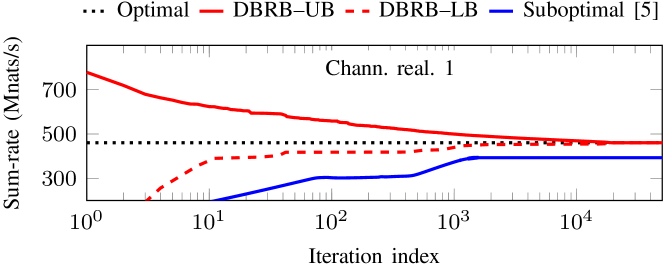
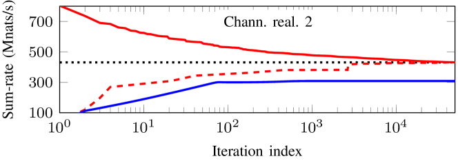
Fig. 1: Convergence behavior of the DBRB and comparison to the suboptimal one in [5] for two channel realizations with $\bar{C}=200$ Mnats/s.

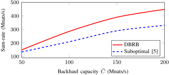
Fig. 2: Average sum rate versus the backhaul capacity $\bar{C}$.

We numerically evaluate the proposed DBRB method. We consider a network consisting of $B=3$ BSs equipped by $M=4$ antennas and $K=6$ single-antenna users randomly placed in the coverage area of all BSs. The inter-site distance between two BSs is $d=1$ km. The pathloss model is given by $\text{PL(dB)}=128.1+37.6\log_{10}(d)$ and the standard deviation of the log normal shadowing is 8. The transmit power budget is $\bar{P}=46$ dBm, the noise power density is $N_{0}=-174$ dBm/Hz and the system bandwidth is $W=10$ MHz. We also set the per-user specified SINR $\bar{\gamma}_{0}=0$ dB. For comparison purposes, we use Alg. 1 as a benchmark to the suboptimal method studied in [5] which measures the same backhaul metric as this paper.

Fig. 1 shows examples of the convergence behavior of the DBRB algorithm, i.e., the convergence is declared when the gap between upper bound (UB) and lower bound (LB) is small enough. As can be seen, this gap is reduced rapidly during first few iterations since a large number of infeasible portions are cut off. Alg. 1 converges after a finite number of iterations. Another interesting observation is that the performance of the solution in [5] is quite far from the optimal one. This can also be seen by Fig. 2 where we illustrate the average sum rate versus the backhaul capacity. Fig. 2 demonstrates that the suboptimal method only attains 70% to 90% of the optimal performance. Thus, there is a need of a more efficient low-complexity scheme.

5 Conclusion

This paper has considered the problem of joint beamforming and BS-user link selection to maximize the sum rate in a downlink CoMP transmission with limited backhaul capacity links. We have derived an optimization framework that solves the design problem to global optimality by customizing a DBRB algorithm. We have also numerically shown the finite convergence of the proposed method. The proposed optimal solution serves as a benchmark and can generate design guidelines for the suboptimal solutions. The DBRB framework can be extended for similar problems involving different backhaul usage measures.

References

- [1] D. Gesbert, S. Hanly, H. Huang, S. Shamai Shitz, O. Simeone, and W. Yu, “Multi-cell MIMO cooperative networks: A new look at interference,” IEEE J. Sel. Areas Commun., vol. 28, no. 9, pp. 1380–1408, Dec. 2010.
- [2] Patrick Marsch and Gerhard P Fettweis, Coordinated Multi-Point in Mobile Communications: from theory to practice, Cambridge University Press, 2011.
- [3] C. Yang, S. Han, X. Hou, and A. F. Molisch, “How do we design CoMP to achieve its promised potential?,” IEEE Wireless Commun., vol. 20, no. 1, pp. 67–74, February 2013.
- [4] O. Tipmongkolsilp, S. Zaghloul, and A. Jukan, “The evolution of cellular backhaul technologies: Current issues and future trends,” IEEE Commun. Surveys Tuts., vol. 13, no. 1, pp. 97–113, First 2011.
- [5] B. Dai and W. Yu, “Sparse beamforming and user-centric clustering for downlink cloud radio access network,” IEEE Access, vol. 2, pp. 1326–1339, 2014.
- [6] F. Zhuang and V. K. N. Lau, “Backhaul limited asymmetric cooperation for MIMO cellular networks via semidefinite relaxation,” IEEE Trans. Signal Process., vol. 62, no. 3, pp. 684–693, Feb. 2014.
- [7] D. W. K. Ng, E. S. Lo, and R. Schober, “Energy-efficient resource allocation in multi-cell OFDMA systems with limited backhaul capacity,” IEEE Trans. Wireless Commun., vol. 11, no. 10, pp. 3618–3631, Oct. 2012.
- [8] J. Zhao, T. Q. S. Quek, and Z. Lei, “Coordinated multipoint transmission with limited backhaul data transfer,” IEEE Trans. Wireless Commun., vol. 12, no. 6, pp. 2762–2775, June 2013.
- [9] A. Wiesel, Y. Eldar, and S. Shamai, “Linear precoding via conic optimization for fixed MIMO receivers,” IEEE Trans. Signal Process., vol. 54, no. 1, pp. 161–176, Jan. 2006.
- [10] P. T. Khoa, T. T. Son, H. D. Tuan, and H. Tuy, “Monotonic optimization based decoding for linear codes,” in 2006 IEEE International Conference on Acoustics Speech and Signal Processing Proceedings, May 2006, vol. 4, pp. IV–IV.
- [11] Y. J. Zhang, L. Qian, and J. Huang, “Monotonic optimization in communication and networking systems,” Found Trends ®Networking, vol. 7, no. 1, pp. 1–75, 2013.
- [12] E. Che, H. D. Tuan, and H. H. Nguyen, “Joint optimization of cooperative beamforming and relay assignment in multi-user wireless relay networks,” IEEE Trans. Wireless Commun., vol. 13, no. 10, pp. 5481–5495, Oct 2014.
- [13] H. Tuy, F. Al-Khayyal, and P. T. Thach, “Monotonic optimization: Branch and cut methods,” in Essays and Surveys in Global Optimization, pp. 39–78. Springer, 2005.
- [14] H. Tuy, M. Minoux, and N.T Hoai-Phuong, “Discrete monotonic optimization with application to a discrete location problem,” SIAM Journal on Optimization, vol. 17, no. 1, pp. 78–97, 2006.
- [15] F. A. Al-Khayyal and J. E. Falk, “Jointly constrained biconvex programming,” Mathematics of Operations Research, vol. 8, no. 2, pp. 273–286, 1983.