Turbulent gas accretion between supermassive black holes and star-forming rings in the circumnuclear disk

While supermassive black holes are known to co-evolve with their host galaxy, the precise nature and origin of this co-evolution is not clear. We here explore the possible connection between star formation and black hole growth in the circumnuclear disk (CND) to probe this connection in the vicinity close to the black hole. We adopt here the circumnuclear disk model developed by Kawakatu & Wada (2008) and Wutschik et al. (2013), and explore both the dependence on the star formation recipe as well as the role of the gravitational field, which can be dominated by the central black hole, the CND itself or the host galaxy. A specific emphasis is put on the turbulence regulated star formation model by Krumholz & McKee (2005) to explore the impact of a realistic star formation recipe. It is shown that this model helps to introduce realistic fluctuations in the black hole and star formation rate, without overestimating them. Consistent with previous works, we show that the final black hole masses are rather insensitive to the masses of the initial seeds, even for seed masses of up to $10^{6}$ M_⊙. In addition, we apply our model to the formation of high-redshift quasars, as well as to the nearby system NGC 6951, where a tentative comparison is made in spite of the presence of a bar in the galaxy. We show that our model can reproduce the high black hole masses of the high-redshift quasars within a sufficiently short time, provided a high mass supply rate from the host galaxy. In addition, it reproduces several of the properties observed in NGC 6951. With respect to the latter system, our analysis suggests that supernova feedback may be important to create the observed fluctuations in the star formation history as a result of negative feedback effects.

1 Introduction

The processes which regulate the co-evolution of supermassive black holes (SMBH) with their host galaxies are still not well understood, as well as the activity of SMBH over cosmological time scales. However, SMBH have been successfully detected both directly and indirectly at the centers of the galaxies, and their masses span from millions to billions of solar masses (Fan et al., 2004, 2006; Mortlock et al., 2011; Venemans et al., 2012; Willott et al., 2003). A widely accepted view suggests that the growth of SMBH occurs due to rapid accretion and merging. However, it is still unclear what physical mechanisms drive SMBH to reach such high masses and what gives rise to the correlation with the physical properties of their host galaxies.

Substantial efforts were undertaken and numerous models have been proposed to explain the origin and formation of SMBH through different mechanisms (Rees, 1984). However, to explain the formation of SMBH at higher redshift requires to study the first black hole (BH) seeds. So far, there are three main scenarios which include the formation of BH seeds through the core collapse of Population III stars (Trenti & Stiavelli, 2007), the collapse of dense stellar clusters (Devecchi et al., 2010, 2012) and the collapse of protogalactic metal free gas clouds in primodial halos (see e.g. Latif & Ferrara, 2016). The latter mechanism provides the potentially largest seed masses, and may thus favor the formation of supermassive black holes at $z>6$ (e.g. Lodato & Natarajan, 2007; Wise et al., 2008; Begelman & Shlosman, 2009; Schleicher et al., 2010a; Latif et al., 2013a, b; Schleicher et al., 2013; Ferrara et al., 2014). These high-redshift black holes can potentially be detected with ALMA using CO and H2 line emission (Spaans & Meijerink (2008); Schleicher et al. (2010b)).

Several studies have found tight correlations between black hole mass and galaxy bulge properties in the nearby universe. Such correlations have indicated scaling relations of black hole mass with bulge mass as well as black hole mass with the velocity dispersions of their host (Magorrian et al. (1998); Haring & Rix (2004) Marconi & Hunt (2003); Merritt (1999); Gebhardt et al. (2000);Ferrarese & Merritt (2000)). Correlations between star formation rate and SMBH growth have also been found by Diamond-Stanic & Rieke (2012). Their work includes a complete sample of Seyfert galaxies and they found a strong correlation between nuclear ($r<1$ kpc) star formation rates and the accretion rates of the SMBH with a scaling relation $\dot{M}_{*}\sim\dot{M}^{0.8}_{\rm{BH}}$. Measurements on scales $r>1$ kpc with extended star formation in the host galaxy showed only a weak correlation and scaling as $M_{*}\sim\dot{M}^{0.6}_{\rm{BH}}$. Their results suggest a connection between gas on sub-kiloparsec scales that is forming stars and the gas on sub-parsec scales that goes into black hole accretion. In this case, the transport of angular momentum in the galactic disk would be a natural mechanism which plays a significant role in feeding the central engine and triggering star formation. Additionally, prominent circumnuclear disks with star formation rings have been observed in the inner regions of some galaxies from parsec scale up to a few kilo parsecs from the galactic center (Lenc & Tingay, 2009; Hsieh et al., 2011; van der Laan et al., 2013; Falcon-Barroso et al., 2013).

In the last years for several active galaxies gas mass inflows to the nucleus have been detected through optical and near-infrared spectroscopy with estimated inflow rates of the order of $10^{-2}M_{\odot}yr^{-1}$ (Schnorr-Müller et al., 2016; Lena et al., 2015; Schnorr-Müller et al., 2014a, b; Storchi-Bergmann et al., 2009, 2010). However, from the current observations it is difficult to determine the actual kinematics of the inflowing gas to the nucleus (Storchi-Bergmann et al., 2010).

Co-evolution models and numerical simulations are necessary for explaining and describing the processes that regulate and control the accretion onto SMBH as well as the gas inflow from the host galaxy which triggers nuclear starbursts from kilo-parsec scale down to parsec scale in active galaxies. Kawakatu & Wada (2008) and Wutschik et al. (2013) have proposed models of co-evolution, where the transport of angular momentum from the outer border of the CND to the SMBH is driven by turbulence injected via supernova explosions that lead to different accretion phases in the disk around a SMBH. An important aspect studied by Wutschik et al. (2013) is the functional form of the star formation rate, as different dependencies have been suggested in the literature with respect to the surface density of the gas as well as the turbulent velocity. The models explored included both linear and nonlinear dependencies on the gas surface density, as well as models independent of the turbulent velocity $\rm{v}_{turb}$ and models where the star formation rate scales as $\rm{v}_{turb}^{-1}$. Specific models adopted from the literature included in particular the model employed by Kawakatu & Wada (2008) and by Elmegreen & Burkert (2010) (hereafter model EB10) .

In this work, we further extend the framework of Wutschik et al. (2013) and apply it to the formation of both nearby AGN and high-redshift quasars. For this purpose, we include the star formation recipe by Krumholz & McKee (2005) (hereafter model KM05), including both non-linear dependencies on gas surface density and turbulent velocity, from which the Kennicutt-Schmidt relation can be derived in a systematic manner. We also explore whether our assumptions regarding the gravitational dynamics have a strong impact on the results. With this new model, we will show that the non-linear dependence in the star formation model, along with feedback from supernova explosions, can give rise to star formation histories that are similar to the observed ones.

In section 2, we describe the general implementation along with the new star formation model considered here. Section 3 shows the results of semi-analytical calculations and simulations which describe the time evolution of the black hole mass, stellar mass and disk radius, exploring different assumptions on the dominant component in the gravitational field. We also show the time evolution of the Mach numbers and the expected evolution of observable quantities as the luminosities. In section 4, the model is then applied to specific objects including local AGN and high-redshift quasars. Finally section 5 presents our discussion and conclusions.

2 Evolution of the SMBH and star formation in a circumnuclear disk

2.1 Disk Model

The co-evolution model of Kawakatu & Wada (2008) considers the following system: an accreting SMBH surrounded by a CND, all embedded in the galaxy. The host galaxy supplies matter (dusty gas) with the rate $\dot{M}_{sup}$ to the CND. The disk becomes gravitationally unstable at a critical radius $r_{c}$, where the Toomre Q parameter is equal to 1. This separates the disk into an outer disk (self-gravitating region) and into an inner disk (stable region). In the gravitationally unstable outer disk stars are forming and the turbulent pressure produced by supernova explosions drives gas to the inner disk to feed the SMBH.

In the extension of the model by Wutschik et al. (2013) (hereafter model WS13), the stable and the unstable part of the CND are treated separately, assuming a power-law surface density distribution where the power-law index is obtained from normalization constraints. The mass exchange between both parts of the disk is driven by direct mass exchange due to accretion from the unstable outer disk to the inner disk, as well as through geometric effects, i.e. if the critical radius moves towards the inner or outer part of the disk. The model also includes the cases where the entire CND is stable or unstable, i.e. where the critical radius is equal to the inner or outer radius of the CND (see also Kawakatu & Wada (2008)). Wutschik et al. (2013) and Kawakatu & Wada (2008) show that depending on the stability of the CND, one can distinguish between the following phases:

a) High accretion phase (constant supply from the host galaxy):

• Due to higher matter density or lower turbulent velocity, stable matter in the disk becomes unstable , which results into the critical radius moving inward, i.e. $r_{c}(t_{o})>r_{c}(t)$ or $r_{c}\leq r_{in}$.

• In consequence, gas $\Delta M_{g}$ from the inner gas reservoir flows to the outer reservoir. Hence the gas mass in the outer region $M_{g,o}$ is defined as $M_{g,o}(t)=M_{g,o}(t_{o})-\Delta M_{g}$.

• The disk becomes geometrically thick, stars form and their feedback through supernova explosions leads to the turbulent supersonic phase. In this phase, the disk thickness is regulated by the turbulent pressure of the gas $P_{g}$ which is defined as $P_{g}=\rho_{g}v^{2}_{turb}$, where $\rho_{g}$ is the gas density and the turbulent velocity $v_{turb}$ is generally larger than the sound speed $c_{s}$, i.e. $v_{turb}>c_{s}$.

• The turbulent energy in the disk is $E_{turb}(r)=\Sigma_{g}v^{2}_{turb}(r)$, where $\Sigma_{g}$ is the surface density of the gas.

• The total energy injected by supernovae is given as $\dot{E}_{inj}(r,t)=f_{SN}\eta_{SN}E_{SN}\hat{{{\dot{\Sigma}}}}_{*}(r,t-t_{SN})$, with $t_{SN}$ is the average life-time of massive stars which then explode into supernovae, $E_{SN}$ the energy injected into the ISM via supernova, $\eta_{SN}$ the heating efficiency. and $f_{SN}$ is a constant parameter. $\hat{{{\dot{\Sigma}}}}_{*}(r,t-t_{SN})$ is the local star formation rate per unit area. We assume here that the energy not going into turbulence is dissipated ($E_{dis}$) through other processes, and due to the energy balance, we then have $\dot{E}_{turb}(r)+\dot{E}_{dis}(r)=\dot{E}_{inj}$. As a typical lifetime for massive stars, we adopt $10^{6}$ years, but we will also explore variations of this parameter in section 4.

• The feedback from supernova explosions is the primary mechanism which drives the gas to the inner disk to feed the black hole. During this phase, accretion becomes highly efficient.

b) Low accretion phase (after termination of supply from host galaxy):

• Gravitationally unstable matter in the disk (in a state of active star formation) becomes stable which results into the critical radius moving outward, i.e. $r_{c}(t_{o})<r_{c}(t)$ or $r_{c}>r_{in}$.

• The gas reservoir of the inner stable disk therefore increases, as a larger part of the CND is becoming stable over time.

• Once stable, the disk is vertically supported only by thermal gas pressure, $P_{g}=\rho_{g}c^{2}_{s}$, where $v_{turb}<c_{s}$.

• The scale height of the disk is determined by the balance between gravity and thermal gas pressure. Accretion is inefficient in this phase.

In our model we employ the input parameters for the outer and inner radius of the disk as $r_{out}=\sqrt{M_{BH}/\pi\Sigma_{host}}$ and $r_{in}=3pc\sqrt{M_{BH}/10^{8}M_{\odot}}$ respectively (Wutschik et al., 2013; Kawakatu & Wada, 2008). Table  1 summarizes the fixed and free parameters of our model. The values for the time of supply $t_{sup}$, the surface density of the host galaxy $\Sigma_{host}$, the power law exponent for the surface gas density $\gamma$, the parameters related to the energy injected by supernova explosions ($t_{SN}$, $f_{SN}$, $\eta_{SN}$ and $E_{SN}$), and the thermal sound speed $c_{s}$ are taken from previous works (Wutschik et al., 2013; Kawakatu & Wada, 2008). Considering mass conservation, the mass balance in the system is $M_{sup}=M_{BH}+M_{g}+M_{\ast}$, where $M_{sup}$ is the mass supplied to the CND, $M_{BH}$ is the black hole mass, $M_{g}$ is the gas mass and $M_{\ast}$ is the stellar mass. The time evolution of the gas mass in the disk is given as

$$M_{g}(t)=\int_{0}^{t}[\dot{M}_{sup}(t^{\prime})-\dot{M}_{*}(t^{\prime})-\dot{M}_{BH}(t^{\prime})]\,dt^{\prime},$$ (1)

considering the difference between the mass that was supplied and the mass going into stars and the central black hole. $\dot{M}_{sup}$ is the mass supply rate, $\dot{M}_{BH}$ is the black hole accretion rate and $\dot{M}_{*}$ is the star formation rate in the disk. The latter is given by the following expression:

$$\dot{M}_{*}(t)=\int_{r_{min}}^{r_{out}}2\pi r\dot{\Sigma}_{*}(r)\,dr,$$ (2)

where the value of $r_{min}$ depends also on the disk stability and is given by $r_{min}={\rm max}(r_{in},r_{c})$. To estimate the black hole mass accretion rate in a viscous accretion disk, we refer to the expression given by Pringle (1981) as

$$\dot{M}_{BH}(r,t)=2\pi\nu\Sigma_{g}(r)\frac{d\ln\Omega(r)}{d\ln r},$$ (3)

where $\nu=\alpha{\rm{v}(r)}h(r)$ denotes the viscosity, with $\alpha$ the viscous coefficient, $\rm{v}(r)$ the gas velocity, and $h(r)$ the scale height of the disk. Here $\Omega$ represents the angular velocity of the gas, which is obtained from the balance between the centrifugal force and the gravitational force. The latter depends on the dominant gravitational component, which can be the black hole, the CND itself and the host galaxy. In the general case, it is thus given as

$$\Omega^{2}(r)=\frac{GM_{BH}}{r^{3}}+\frac{\pi G}{r}(\Sigma_{disk}(r)+\Sigma_{host}),$$ (4)

where $\Sigma_{host}$ is the host galaxy surface density, $\Sigma_{disk}=\Sigma_{g}+\Sigma_{stars}$ is the disk surface density. It follows a power law function of the radius, represented as $\Sigma_{disk}\approx\Sigma_{g}=\Sigma_{0}(r/r_{c})^{-\gamma}$, where $\gamma$ is a free parameter (Wutschik et al., 2013). The evolution of the black hole mass $M_{BH}$ from an initial seed mass $M_{BH,seed}$ is given as

$$M_{BH}(t)=M_{BH,seed}+\int_{0}^{t}\dot{M}_{BH}(t^{\prime})\,dt^{\prime}.$$ (5)

Table 1: Model parameters.

Type	Name	Values	fix/free
$\dot{M}_{sup}$	Mass supply rate	1 $M_{\odot}$ $\rm{yr}^{-1}$	free
$t_{sup}$	Time supply in years	$10^{8}$ yr	free
$t_{max}$	Maximum time for iteration	$10^{9}$ yr	free
$\Sigma_{host}$	Host surface density of gas	$10^{4}$ $M_{\odot}$ $\rm{pc}^{-2}$	free
$\alpha$	Viscosity coefficient	1	free
$\gamma$	Gas surface density power law exponent	1	fix
$M_{BH,seed}$	Black hole seed	$10^{3}$ $M_{\odot}$	free
$t_{SN}$	Average life time of massive stars	$\approx 10^{6}$ yr	free
$f_{SN}$	Supernovae rate per solar mass of formed stars	$7.9\times 10^{-3}$	fix
$\eta_{SN}$	supernova heating efficiency	0.1	fix
$E_{SN}$	Thermal energy by core-collapse supernovae	$10^{51}$ erg/s	fix
$c_{s}$	Sound speed	1 km/s	fix
$f_{\rm{GMC}}$	Fraction of molecular clouds	0.5	fix
$Q$	Toomre parameter	1	fix
$\Psi$	Dependent on $f_{\rm{GMC}}$ and $Q$	0.1224	fix

2.2 Star formation rate model

As a new ingredient in our model, we consider here the star formation model of KM05 due to its effective applicability not only to the Milky Way’s star formation rate but also to a vast variety of galaxies and its consistency with observations and simulations. The model particularly allows to derive the two forms of the Kennicutt-Schmidt relation and successfully predicts star formation rates based on observable quantities over a large range of conditions, spanning from normal galactic disks, circumnuclear starburts and ULIRGs to nearby star-forming galaxies such as Markarian 273, Arp 193 and Arp 220.

In the analytical description of KM05, the main premise is that the gas collapses in sub-regions of molecular clouds in a supersonically turbulent environment to form stars. The total star formation rate $\dot{\Sigma}_{*}$ is formulated in terms of the observable properties of the gas in the galactic disk as follows

$$\dot{\Sigma}_{*}\approx 0.073\textit{M}^{-0.32}\phi^{1/2}_{\rho}Q^{-1}_{1.5}f_{\rm{GMC}}\Omega\Sigma_{g}\left[M_{\odot}\rm{pc^{-2}yr^{-1}}\right],$$ (6)

where M is the mach number which is the ratio of the turbulent velocity $\rm{v}_{turb}$ to the local sound speed $c_{s}$. The observable parameter $\phi_{\rho}$ is given by the ratio of the mean molecular density to the mean midplane density. This ratio has been approximated as $5(\phi_{\bar{P}}/6)^{3/4}$, where $\phi_{\bar{P}}\approx 10-8f_{\rm{GMC}}$ (Krumholz & McKee, 2005). The latter can be expressed as $\phi_{\bar{P}}\approx 5[\frac{10-8f_{GMC}}{6}]^{3/4}$, where $f_{\rm{GMC}}$ is the molecular gas fraction. $f_{\rm{GMC}}=0.5$ (it implies $\phi_{\rho}=0.6$) is considered as an universal parameter which applies from starbursts to normal galaxies, as stated in the appendix B of Krumholz & McKee (2005). The parameter $Q$ represents the Toomre parameter (Toomre, 1964; Rice, 2016) in equation (6), $Q_{1.5}=Q/1.5$.

To evaluate the effect of the star formation model on the BH accretion rate and on the star formation rate evolution in the CND, we re-write equation (6) by emphasizing the dependence of the star formation rate on the turbulent velocity and angular velocity:

$$\dot{\Sigma}_{*}(r)=\Psi\Omega(r)\left(\frac{\rm{v}_{turb}(r)}{c_{s}}\right)^{-0.32}\Sigma_{g}(r).$$ (7)

We write the fix parameter $\Psi$ in terms of $Q$ and $f_{\rm{GMC}}$ as $\Psi=0.073\sqrt{5}\left(\frac{10-8f_{\rm{GMC}}}{6}\right)^{3/8}\dfrac{1.5}{Q}f_{\rm{GMC}}$. Now that we have condensed equation (6), we employ in the next section the formulation given in equation (7) for studying the evolution of the circumnuclear disk. If (part of) the CND is gravitationally unstable, the turbulent velocity in this region will be calculated based on the energy input from supernovae, leading to supersonic turbulence. As in the WS13 model, we approximate the turbulent velocity here as a power law via

$$\rm{v}_{turb}={\rm{v}}_{o}\left(\frac{r}{r_{out}}\right)^{\lambda},$$ (8)

where $\rm{v}_{o}=\sqrt{E_{turb}(r_{c})/\Sigma_{g}(r_{c})}$ and $\lambda$ is the power law index expressed as $\lambda=\dfrac{1.5-\gamma(\theta-1)}{(2+\epsilon)}$, which is 0 in the sub-sonic turbulence phase. The parameters $\theta$ and $\epsilon$ come from the parametrization of the total star formation rate as $\dot{\Sigma}_{*}(r)=\Psi\cdot\left(\Sigma_{g}(r)\right)^{\theta}\cdot(\rm{v}_{turb})^{-\epsilon}$ (Wutschik et al., 2013) . In the KM05 model the latter two parameters have the values of 1 and 0.32 respectively (see equation (7)), hence we use them for calculating the value of $\lambda$, which is approximately equal to 0.65.

2.3 Dependence of accretion on dominant gravitational source

As described in section 2.2, the total star formation rate depends non-linearly on the turbulent velocity and linearly on the surface density of gas. However, since in equation (4) the angular velocity depends on different gravitational source terms, we insert this relation into equation (7) to write the total star formation rate as

$$\footnotesize\dot{\Sigma}_{*}(r) =\Psi\sqrt{{\frac{GM_{BH}}{r^{3}}+\frac{\pi G}{r}\left(\Sigma_{disk}(r)+\Sigma_{host}\right)}}\cdot$$

$$\phantom{{}=1}\left(\frac{{\rm{v}_{turb}}(r)}{c_{s}}\right)^{-0.32}\Sigma_{g}(r).$$ (9)

To evaluate the evolution of the star formation rate $\dot{M}_{*}(t)$ in the CND, one has to insert equation (2.3) into (2). To calculate equation (2) analytically, we first consider three different limiting cases of $\dot{\Sigma}_{\ast}(r)$, depending on the dominant source of gravity in the system: the central black hole, the CND itself or the gravitational field from the host galaxy. As a result, we will obtain expressions for the star formation rate $\dot{M}_{*}(t)$ and the energy injection rate $\dot{E}_{inj}$ in different regimes.

If gravity is dominated by the central black hole, we obtain $\dot{\Sigma}_{*}(r)=\Psi\sqrt{\left(\frac{GM_{BH}}{r^{3}}\right)}\left(\frac{\rm{v}_{turb}(r)}{c_{s}}\right)^{-0.32}\Sigma_{g}(r)$, and the analytic solution for $\dot{M}_{*}(t)$ and $\dot{E}_{inj}$ is given as

$$\dot{M}_{*}(t) =\frac{2\pi\Psi\sqrt{GM_{BH}}}{\frac{1}{2}-\theta\gamma-\epsilon\lambda}\Sigma^{\theta}_{o}\left(\frac{\rm{v}_{o}}{c_{s}}\right)^{-\epsilon}\cdot$$

$$\phantom{{}=1}r^{\theta\gamma+\epsilon\lambda}_{c}\left[r^{\frac{1}{2}-\theta\gamma-\epsilon\lambda}_{out}-r^{\frac{1}{2}-\theta\gamma-\epsilon\lambda}_{c}\right],\rm{and}$$ (10)

$$\dot{E}_{inj} =7.9\cdot 10^{-3}\eta_{SN}E_{SN}\frac{\dot{M}_{*}}{2\pi}\left(\frac{1}{2}-\theta\gamma-\epsilon\lambda\right)\cdot$$

$$\phantom{{}=1}r^{-\theta\gamma-\epsilon\lambda-\frac{3}{2}}\left[r^{\frac{1}{2}-\theta\gamma-\epsilon\lambda}_{out}-r^{\frac{1}{2}-\theta\gamma-\epsilon\lambda}_{in}\right]^{-1}.$$ (11)

If the gravitational force is dominated by the CND itself, then $\dot{\Sigma}_{*}(r)=\Psi\sqrt{\left(\frac{\pi G\Sigma_{disk}}{r}\right)}\left(\frac{\rm{v}_{turb}(r)}{c_{s}}\right)^{-0.32}\Sigma_{g}(r)$, and the analytic solution for $\dot{M}_{*}(t)$ and $\dot{E}_{inj}$ follows as

$$\dot{M}_{*}(t) =\frac{2\pi\Psi\sqrt{G\pi\Sigma_{o}}}{\frac{3}{2}-\gamma(\frac{1}{2}+\theta)-\epsilon\lambda}\Sigma^{\theta}_{o}\left(\frac{\rm{v}_{o}}{c_{s}}\right)^{-\epsilon}r^{\theta\gamma+\epsilon\lambda+\frac{\gamma}{2}}_{c}\cdot$$

$$\phantom{{}=1}\left[r^{\frac{3}{2}-\gamma(\frac{1}{2}+\theta)-\epsilon\lambda}_{out}-r^{\frac{3}{2}-\gamma(\frac{3}{2}+\theta)-\epsilon\lambda}_{c}\right],\rm{and}$$ (12)

$$\dot{E}_{inj} =7.9\cdot 10^{-3}\eta_{SN}E_{SN}\frac{\dot{M}_{*}}{2\pi}\left(\frac{3}{2}-\gamma(\frac{1}{2}+\theta)-\epsilon\lambda\right)\cdot$$

$$\phantom{{}=1}r^{-\gamma(\frac{1}{2}+\theta)-\epsilon\lambda-\frac{1}{2}}\left[r^{\frac{3}{2}-\gamma(\frac{3}{2}+\theta)-\epsilon\lambda}_{out}-r^{\frac{3}{2}-\gamma(\frac{1}{2}+\theta)-\epsilon\lambda}_{in}\right]^{-1}.$$ (13)

Finally if gravity is dominated by the host galaxy, the star formation rate is expressed as $\dot{\Sigma}_{*}(r)=\Psi\sqrt{\left(\frac{\pi G\Sigma_{host}}{r}\right)}\left(\frac{\rm{v}_{turb}(r)}{c_{s}}\right)^{-0.32}\Sigma_{g}(r)$, and the analytical solution for $\dot{M}_{*}(t)$ and $\dot{E}_{inj}$ is given as

$$\dot{M}_{*}(t) =\frac{2\pi\Psi\sqrt{G\pi\Sigma_{host}}}{\frac{3}{2}-\theta\gamma-\epsilon\lambda}\Sigma^{\theta}_{o}\left(\frac{\rm{v}_{o}}{c_{s}}\right)^{-\epsilon}r^{\theta\gamma+\epsilon\lambda}_{c}\cdot$$

$$\phantom{{}=1}\left(r^{\frac{3}{2}-\theta\gamma-\epsilon\lambda}_{out}-r^{\frac{3}{2}-\theta\gamma-\epsilon\lambda}_{c}\right),\rm{and}$$ (14)

$$\dot{E}_{inj} =7.9\cdot 10^{-3}\eta_{SN}E_{SN}\frac{\dot{M}_{*}}{2\pi}\left(\frac{3}{2}-\theta\gamma-\epsilon\lambda\right)\cdot$$

$$\phantom{{}=1}r^{-\theta\gamma-\epsilon\lambda-\frac{1}{2}}\left[r^{\frac{3}{2}-\theta\gamma-\epsilon\lambda}_{out}-r^{\frac{3}{2}-\theta\gamma-\epsilon\lambda}_{in}\right]^{-1}.$$ (15)

In the most general case, different regimes (where different terms in the gravitational field may become dominant in different parts of the CND), and their evolution may further be time-dependent. As we aim here to work with a still simplified model, we will thus show in the following that the results are not highly sensitive to the choice of the gravitational force term.

Figure 1: Final black hole (markers) and stellar (lines) masses under different assumptions for the gravitational field, and as a function of the mass supply rate. Results from the KM05 model with the gravitational field dominated by the central black hole (circle and line), by the CND (square and dotted line), by the host galaxy (diamond and dotted-dashed line). In addition results for the EB10 model, assuming the CND as the gravitational source (red crosses and red dashed line).

3 Results

3.1 Evolution of the SMBH accretion rate, the star formation rate and masses

The model described in the previous sections allows us to explore the evolution of different physical quantities of the system that include the evolution of the black hole growth from an initial seed, the evolution of the star formation rate taking place on the outer disk, the evolution of the gas velocity as well as the AGN luminosity. In general, in this model we adopt a marginally stable self-gravitating disk $Q\approx 1$ (consistent with Wutschik et al., 2013) and the universal fraction of molecular clouds ($f_{\rm{{GMC}}}=0.5$ as shown by Krumholz & McKee, 2005).

As mentioned in the previous section, we examine the impact of the star formation model KM05 on the evolution of the system. Figure 1 compares the final black hole mass and final stellar mass as a function of the mass supply rate $M_{\odot}$ under different assumptions for the dominant gravitational source, using simulations with the input parameters displayed in table 1. It can be seen that the final stellar masses are independent on the assumptions regarding the gravitational field. The black hole mass depends somewhat on the underlying gravitational field, but the difference amounts to only a factor of a few. Additionally, in figure 1 we compare our results produced with the KM05 model with the results produced with the EB10 model.

We note here that by setting an initial black hole seed of $10^{3}$ $M_{\odot}$ and having a $\dot{M}_{sup}\geq 100$ $M_{\odot}$ $\rm{yr}^{-1}$ from the galaxy to the circumnuclear disk, both models KM05 and EB10 enable the growth of supermassive black hole mass to the order of $10^{9}$ $M_{\odot}$. It is interesting to note that the final black hole masses converge to similar values both in the KM05 model and the EB10 model, here explored in the limit where the CND dominates the gravitational field.

Although both models KM05 and EB10 produce similar final masses, model KM05 produces more stable accretion during the high accretion phase whereas model EB10 produces over-accretion during that phase (see figure 2). Stable accretion is reflected as less sharp fluctuations on the accretion rate and on the star formation rate in the period of $10^{6}$ to $10^{7}$ years. This effect is also reflected in the turbulent Mach number, which is driven by the feedback from star formation. Compared to the EB10 model, the dependence on the turbulent velocity is however less severe, scaling as $M^{-0.32}$ rather than $M^{-1}$, thus reducing the impact of the negative feedback and damping the fluctuations within the system. In addition, as already described by Wutschik et al. (2013), there are hints of anticyclic variations between the black hole accretion rate and the star formation rate, which may be interpreted as competition between gas consuming processes in the CND.

Table 2: Dependence of final black hole masses on initial seed, mass supply rate and dominant gravitational field.

Final black hole mass [$10^{7}$ $M_{\odot}$]
Supply rate [$M_{\odot}\rm{yr}^{-1}$]	Seed $[M_{\odot}]$	BH field	Host field	Disk field
1	$10^{3}$	2.95	1.82	3.09
	$10^{6}$	2.96	1.86	3.13
10	$10^{3}$	23.3	77.5	15.6
	$10^{6}$	23.4	77.8	15.6
100	$10^{3}$	118	319	733
	$10^{6}$	118	319	733

Figure 2: Time evolution of $\dot{M}_{BH}(t)$, $\dot{M_{*}}(t)$, $M(t)$ associated to model EB10 (red line), and model KM05 (black line) for a gravitational field dominated by the black hole.

We have also investigated the influence of the black hole seed mass on the system’s evolution. For this purpose, table 2 compares the final black hole masses at adopting different seeds and under different assumptions regarding the central source of gravity. In all cases, it is clearly visible that the final black hole mass has an extremely weak dependence on the mass of the initial seed, even when considering seed masses of $10^{6}$ $M_{\odot}$, which are at the upper limit of what is suggested in the literature. This has been reported already by Armijo & Pacheco (2011), and Wutschik et al. (2013), the last one adopts different assumptions on star formation. However, as it was shown in figure 1, a large mass supply rate to the system indeed enhances the final black hole masses. For instance for a supply rate of 100 $M_{\odot}$ $\rm{yr}^{-1}$, the final masses are of the order of $10^{9}$ $M_{\odot}$ which is in agreement with the results given by Volonteri et al. (2015). While for moderate mass supply rates of 1$M_{\odot}$ yr^-1 and 10 $M_{\odot}$ yr^-1, the final black hole masses also just weakly depend on our assumptions concerning the gravitational acceleration, they differ by roughly a factor of 3 when considering large supply rates of 100 $M_{\odot}$ yr^-1.

3.2 Evolution of the Mach number

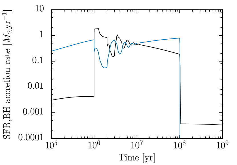
Figure 11: Time evolution of the black hole (BH) mass accretion rate (black line) and star formation rate (SFR) (blue line) with gravity dominated by the central black hole, assuming a mass supply rate of 1 $M_{\odot}$ $\rm{yr}^{-1}$.

Figures 6, 6, and 6 show the time evolution of the Mach number for different mass supply rates under different assumptions of the central gravitational field. We note in general that the turbulent velocity of the gas becomes larger compared to the local sound speed during the high accretion phase (starting at $10^{6}$ years), which leads to large Mach numbers. When comparing the Mach number evolution in the different dominant gravitational scenarios, we notice that it is highest when the gravitational field is dominated by the central black hole, with $M_{\rm{max}}\approx 65$ at $\dot{M}_{sup}=$1 $M_{\odot}$ $\rm{yr}^{-1}$. In this scenario, the black hole accretes efficiently with $\dot{M}_{\rm{BH}}\approx$ 1$M_{\odot}$ $\rm{yr}^{-1}$(see also Fig. 11).

When the gas supply ceases after $10^{8}$ years, the gas accretion becomes less efficient, so the black hole accretes afterwards at very low rates (see figure 12). At this timescale, a very pronounced spike appears on the Mach number evolution at all field dominations. The latter is a result of delayed supernova feedback at a time where the supply of new gas is inhibited, thus strengthening the effect of the feedback. Subsequently, on a timescale comparable to the lifetime of massive stars, the Mach number drops to a value of order unity, as turbulence is no longer driven by supernovae, but may result from hydrodynamical instabilities.

In the simulations presented here, the value of the viscosity coefficient $\alpha$ was of the order of unity in all our simulations. However, this quantity is still uncertain, and it is worth mentioning that Kawakatu & Wada (2008), and Wutschik et al. (2013) have associated different values of $\alpha$ to the different accretion phases. In their assumptions, $\alpha$ has the order of unity in the turbulent supersonic phase whereas in the subsonic phase $\alpha\approx 0.01-0.5$ (due to magneto-rotational instabilities) where the turbulent velocity is comparable to the local sound speed. To study the dependence of our results on $\alpha$, we have run simulations to compare different values of $\alpha$ with $\alpha={0.01,0.5,1}$. Figure 6 shows the time evolution of the Mach number for the different values of $\alpha$. It can be seen that small values of $\alpha<1$ have a weak impact on the accretion phases, i.e. the gas velocity remains comparable to the sound speed during the subsonic phase. Additionally, the Mach number evolution follows the same trend for all values of $\alpha$ except that it reduces very slightly the Mach numbers in the period of 1 million, and 3 million years. We find here that the time evolution of the BH accretion rate, star formation rate, final masses, and radius are quite independent of the parameter $\alpha$. Such independence on $\alpha$ shows that the accretion is dynamically regulated by the available mass reservoir, and therefore remains efficient as long as sufficient matter will be available.

3.3 Evolution of the CND radii

Returning to the evolution of the accretion disk itself, we have also studied the evolution of the final inner and outer radius as a function of time and mass supply rate (see figures 10 to 10), exploring different assumptions regarding the gravitational field. The explored mass supply rates ranging from 1 to 1000 $M_{\odot}$ $\rm{yr}^{-1}$ allow the rapid growth of the disk radii from parsec to kiloparsec scale. We find no significant dependence of the final values of the outer radius on the assumption regarding the gravitational field. So the results converge to similar values after the gas supply ceases at $10^{8}$ years. The final outer radius is comparable for instance with the size of some circumnuclear rings in galaxies like NGC 1097 with 1.5 kpc of radius studied by Hsieh et al. (2011) and NGC 613 with a nuclear starburst of 700 pc wide found by Falcon-Barroso et al. (2013). The inner radius, on the other hand, always remains at similar values, with distances from the center spanning from 1 to approximately up to 30 pc.

Figure 3: Mach number evolution with gravity dominated by the central black hole for different mass supply rates: 1 $M_{\odot}$ yr^-1 (line),  10 $M_{\odot}$ $\rm{yr}^{-1}$ (dashed line), 100 $M_{\odot}$ $\rm{yr}^{-1}$ (dotted line).

Figure 4: Mach number evolution with gravity dominated by the CND for different mass supply rates: 1 $M_{\odot}$ $\rm{yr}^{-1}$(line), 10 $M_{\odot}$ $\rm{yr}^{-1}$(dashed line), 100 $M_{\odot}$ $\rm{yr}^{-1}$(dotted line).

Figure 5: Mach number evolution with gravity dominated by the galactic disk for different mass supply rates: 1 $M_{\odot}$ $\rm{yr}^{-1}$(line), 10 $M_{\odot}$ $\rm{yr}^{-1}$(dashed line), 100 $M_{\odot}$ $\rm{yr}^{-1}$(dotted line).

Figure 6: Mach number evolution with gravity dominated by the central black hole for different viscosity coefficients: $\alpha=1$ (blue line), $\alpha=0.5$ (red line), $\alpha=0.01$ (black line). Here the supply rate is 1$M_{\odot}$ $\rm{yr}^{-1}$.

Figure 7: Disk inner radius vs. mass supply rate with gravity dominated by the central black hole (circles), with by the CND (triangles), and by the host galaxy (inverted triangles).

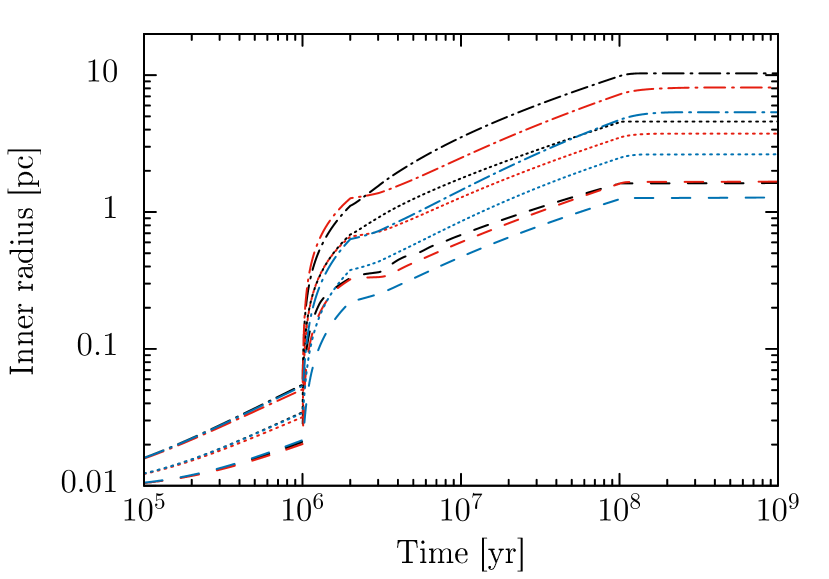
Figure 8: Time evolution of the disk inner radius for different mass supply rates: 1 $M_{\odot}$ $\rm{yr}^{-1}$ (dashed-line) , 10 $M_{\odot}$ $\rm{yr}^{-1}$ (dotted-line), and 100 $M_{\odot}$ $\rm{yr}^{-1}$ (dashed-dotted line) with different assumptions on the central gravitational field: dominated by the central black hole (black color), the CND (red color) and the host galaxy (blue color).

Figure 9: Disk outer radius vs. mass supply rate for gravity dominated by the central black hole (circles), by the CND (triangles) and by the host galaxy (inverted triangles).

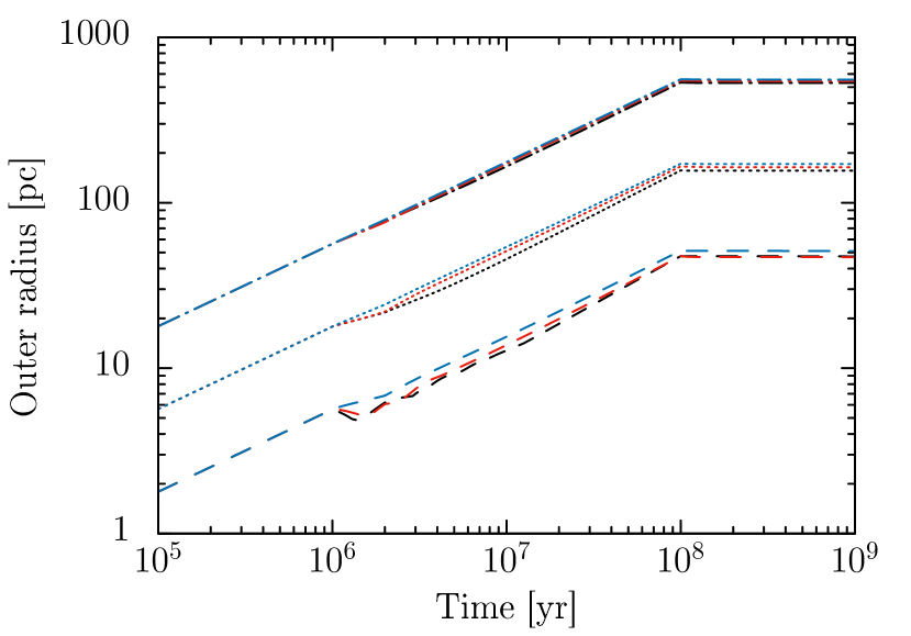
Figure 10: Time evolution of the disk outer radius for different mass supply rates: 1 $M_{\odot}$ $\rm{yr}^{-1}$ (dashed-line) , 10 $M_{\odot}$ $\rm{yr}^{-1}$ (dotted-line) and 100 $M_{\odot}$  $\rm{yr}^{-1}$ (dashed-dotted line) under different assumptions regarding the gravitational field, i.e. dominated by the central black hole (black color), by the CND (red color) and by the host galaxy (blue color).

3.4 Evolution of the luminosities

We also explore here the implications of our model on observable quantities, including the luminosity from the AGN ($L_{\rm{AGN}}$), the nuclear starburst ($L_{\rm{NSB}}$), the stellar luminosity ($L_{\rm{stellar}}$) and for comparison the Eddington luminosity ($L_{\rm{edd}}$). The AGN luminosity is calculated based on two well-known cases: the standard thin disk (Shakura & Sunyaev, 1973) which is applied for the low accretion phase and the slim disks (Abramowicz et al., 1988; Abramowicz, 2004) for the high accretion phase. Similarly as in Kawakatu & Wada (2008), equations (16) and (17) show the dependence of the luminosities on the accretion rate. In the standard disk aproximation, $L_{AGN}$ is given as

$$\rm{L_{AGN}}=\left(\frac{\dot{m}(t)}{10}\right)\rm{L_{edd}(t)},\enspace{\rm\dot{m}(t)<20,}$$ (16)

and in the slim disk approximation $L_{AGN}$ is given as

$$\rm{L_{AGN}}=2\left(1+ln\frac{\dot{m}(t)}{20}\right)\rm{L_{edd}(t)},\enspace{\rm\dot{m}(t)\geq 20},$$ (17)

where $\rm{{\dot{m}}=\frac{\dot{M}_{BH}}{\dot{M}_{edd}}}$, and $\rm{\dot{M}_{edd}=\dot{M}_{crit}=\rm{L_{edd}}/c^{2}}$ (Watarai et al., 2000). The Eddington luminosity $\rm{L_{edd}}$ is given by the following expression:

$$\rm{L_{edd}}=1.25\times 10^{38}\frac{M_{BH}}{M_{\odot}}[erg/s].$$ (18)

For calculating the nuclear starburst luminosity ($\rm{L_{NSB}}$), we adopt the formula given by Kawakatu & Wada (2008), with $\epsilon=0.007$:

$$\rm{L_{NSB}(t)}=0.14\epsilon\dot{M}_{*}(t)c^{2}.$$ (19)

Since our model includes phases without active star formation, we estimate the total stellar luminosity by adopting the mass-to-light ratio ($M/L$) from the total stellar mass. Typical values range from 2 to 10 solar masses per solar luminosity (Dickel, 1978; Faber & Gallagher, 1979). For our calculations we adopt a mass-to-light-ratio of 6 $M_{\odot}/L_{\odot}$.

The curves shown in figure 12 are the results of our simulations for an initial black hole seed mass of $10^{3}$ $M_{\odot}$, with a mass supply rate of 1 $M_{\odot}$ $\rm{yr}^{-1}$. The rest of the input parameters are listed in table 1. Thus figure 12 compares the time evolution of the AGN luminosity, the Eddington luminosity, the nuclear starburst luminosity and the total stellar mass using model KM05 and model EB10. The AGN luminosity is calculated assuming gravity to be dominated by the central black hole. We note that in both models the time evolution of the Eddington luminosities are similar and by comparing them with AGN luminosites, we identify different timescales of the accretion phase: the high accretion phase ($10^{6}-10^{8}$ years) and the low accretion phase ($>10^{8}$ years). We further note that the luminosities should more substantial fluctuations in the model EB10 compared to KM05, which is consistent with the results obtained for the star formation and accretion rates.

These results show that our model predicts upper limits of the luminosities: the highest AGN luminosity ($\sim 10^{45}$ erg/s) and the lowest AGN luminosity ($\sim 10^{42}$ erg/s) as well as the highest nuclear starburst luminosity ($\sim 10^{43}$ erg/s), which are in agreement with Kawakatu & Wada (2008). Furthermore, we note that our model predicts super-Eddington luminosities for the period between $10^{6}$ years and $2\times 10^{7}$ years. Sub-Eddington luminosities occur when the AGN luminosity starts to decrease in the period of $2\times 10^{7}$ years to $10^{8}$ years, then the AGN luminosity drops drastically to lower values after $10^{8}$ years.

In general, we find no significant differences in the time evolution of the total stellar luminosities and Eddington luminosites when models KM05 and EB10 are applied. However, the time evolution of the AGN and nuclear starburst luminosities in both models differs during the high accretion phase. As we have described in section 3.1 model EB10 produces over-accretion during the high accretion phase so in consequence these effect also produces the variabilites on the luminosities displayed in figure 12.

We want to emphasize that the typical timescale for activity in AGN depends on external parameters, and for instance, the external mass supply could last for a shorter time or longer time than $10^{8}$ years. This would depend to some extend on the type of the AGN, the redshift and also the environment. For instance for local AGNs, it may be possible that the accretion phases are typically shorter, while there might be rather long and extended periods of accretion necessary to explain high redshift quasars.

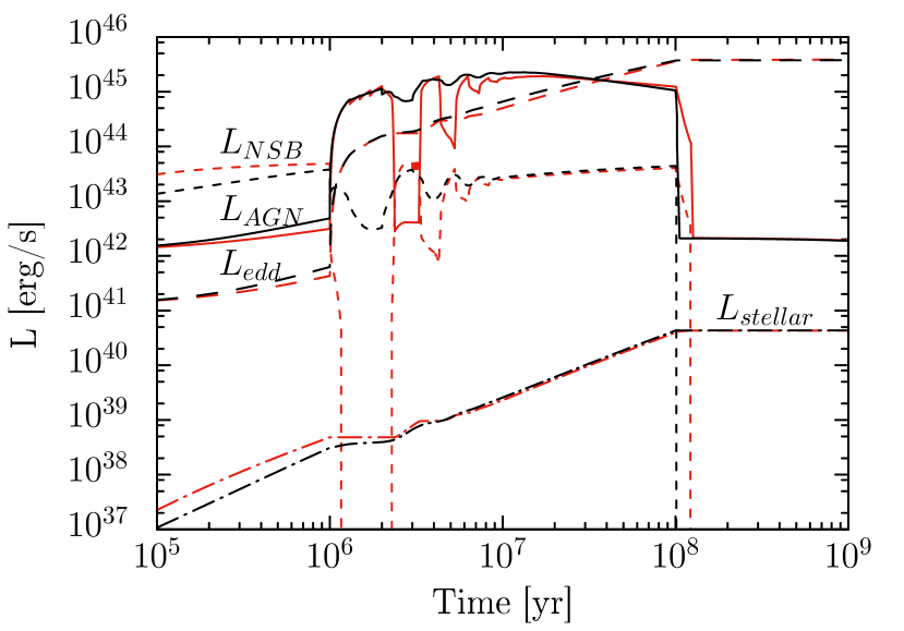
Figure 12: Comparison of the time evolution of the luminosities bewteen model KM05 (black curves) and model EB10 (red curves). The KM05 model is applied with gravity dominated by the central black hole, assuming a mass supply rate of 1 $M_{\odot}$ $\rm{yr}^{-1}$. $\rm{L_{edd}}$ is the Eddington luminosity, $\rm{L_{NSB}}$ the nuclear starburst luminosity, $\rm{L_{AGN}}$ is the AGN luminosity and $\rm{L_{stellar}}$ is the total stellar luminosity.

4 Application of the model to active galaxies and starburst rings

4.1 High redshift quasars

Mortlock et al. (2011) discovered the most distant luminous quasar ULAS J1120+0641, which resides at $z\leavevmode\nobreak\ =7.085$ ($7.6\times\leavevmode\nobreak\ 10^{8}$ years after the big bang). The estimated mass of the supermassive black hole hosted by that quasar is 2 billion solar masses which generates a very large luminosity of $2.4\leavevmode\nobreak\ \times\leavevmode\nobreak\ 10^{47}$ erg/s. Another distant quasar at $z=6.42$, J1148+5251 was discovered by Willott et al. (2003), with a supermassive black hole mass of $4.9\times\leavevmode\nobreak\ 10^{9}$ $M_{\odot}$ and a luminosity of $5.2\times 10^{47}$ $M_{\odot}$ (Pezzulli et al., 2016) (with references therein). We adapt here our model to reproduce the observed AGN properties of these two high redshift quasars. First, we extended the time of mass supply to $8\times 10^{8}$ years, and run simulations for mass supply rates of 30 $M_{\odot}$ $\rm{yr}^{-1}$ and 100 $M_{\odot}$ $\rm{yr}^{-1}$. The rest of the parameters corresponds to the values given in Table 1.

As a result, our model produces final black hole masses of $2.2\times 10^{9}$ $M_{\odot}$ and $4.91\times 10^{9}$ $M_{\odot}$ when the gas supply ceases after $8\times 10^{8}$ years (see figure 15). Such large mass supply rates allow efficient accretion up to 10 $M_{\odot}$ $\rm{yr}^{-1}$ (see figure 15). This large accretion rate lasts only for a short time in the high accretion phase and then produces an upper limit in the luminosity of almost $\sim 10^{47}$ erg/s at roughly $10^{7}$ years (see left graph of figure 15). Shortly after the maximum luminosity is reached, the quasar emits continuous radiation at a rate of $\sim 10^{46}$ erg/s until the gas supply ceases.

We find again that our model predicts super-Eddington and sub-Eddington luminosities even when the time supply is extended up to one billion years. These results are displayed in figure 15, where we compare the time evolution of the luminosities using model KM05 and model EB10 in the same fashion as in figure 12. We note that the application of model EB10 for large accretion rates (¿1 $M_{\odot}$ $\rm{yr^{-1}}$) reduces the over-accretion, but it still produces variations of the AGN and nuclear starburst luminosities during the high accretion phase.

Figure 15 shows that the star formation rate is the preferred mode of gas consumption in the high accretion phase. This effect can be seen in the period of $10^{6}$ years (SN feedback timescale) and $10^{9}$ years, where the evolution of the star formation rate comprises larger and enhanced rates than the BH accretion rates. This behaviour can be attributed to the very large mass supply rate injected from the host galaxy to the outer disk of the CND, where the stars are forming. It is important to note that the injection of a large mass supply rate produces little gas competition between the BH accretion rate and the SFR, whereas for low supply rates, as it was shown in the previous section, a high competition for gas consumption and strong fluctuations develop as displayed in figure 12. Hence, our model predicts an upper limit of the SFR value, which is close to $100$ $M_{\odot}$ $\rm{yr}^{-1}$ (see figure 15). The observed values of the SFR in the quasars at $z=7.085$ and $z=6.42$ are 160 - 440 $M_{\odot}$ $\rm{yr}^{-1}$ and 2000 $M_{\odot}$ $\rm{yr}^{-1}$ respectively, which were estimated both from far-infrared (FRI) luminosities reported by Venemans et al. (2012) and Pezzulli et al. (2016) (with references therein). While the comparison of the SFR values predicted by our model with the observed results shows an apparent discrepancy, one should note that the quoted values of the SFR refer to the entire host galaxy, while our model only follows the evolution in the CND. Higher-resolution observations may however help to constrain the SFR in the central region of the galaxy in the future.

Figure 13: Time evolution of the black hole (BH) masses for different supply rates: 30 $M_{\odot}$ $\rm{yr^{-1}}$ (dashed line) and 100 $M_{\odot}$ $\rm{yr^{-1}}$(dotted line). . When the gas supply ceases at $8\times 10^{8}$ years the final masses are reached.

Figure 14: Black hole (BH) accretion rate (line) and star formation rate (SFR) (dotted-line) evolution for different supply rates. At $8\times 10^{8}$ years, supply rates of 30 $M_{\odot}$ $\rm{yr}^{-1}$(black curves) and 100 $M_{\odot}$ $\rm{yr}^{-1}$ (green curves) produces final black hole masses $2.2\times 10^{9}$ $M_{\odot}$ and $4.9\times 10^{9}$ $M_{\odot}$ respectively.

Figure 15: Comparison of time evolution of the luminosities with model KM05 and model EB10. Left: Model KM05 for different supply rates: 30 $M_{\odot}$ $\rm{yr}^{-1}$ (black curves) and 100 $M_{\odot}$ $\rm{yr}^{-1}$ (green curves). Right: Model EB10 for different supply rates: 30 $M_{\odot}$ $\rm{yr}^{-1}$ (red curves) and 100 $M_{\odot}$ $\rm{yr}^{-1}$ (purple curves).

4.2 The prominent starburst ring in NGC 6951

NGC 6951 is a Seyfert 2 galaxy ($z=0.004750$) with a barred spiral morphology. It exhibits a characteristic starburst ring with radius of 580 pc (van der Laan et al., 2013) but other studies have claimed a radius of 480 pc (Sani et al., 2012). Van der Laan et al. (2013) has determined the stellar content on the circumnuclear rings that spans from young to old stars. The stellar clusters along the ring contain predominantly massive stars with intermediate ages. The total stellar mass estimated in the ring is $6\times 10^{7}$ $M_{\odot}$ with an estimated age between 1 Gyr and 1.5 Gyr. No other determination of the age of the ring has been published so far.

The mass of the central black hole ranges between $5.5\times\leavevmode\nobreak\ 10^{6}$ $M_{\odot}$ at $81^{o}$ and $1.3\times 10^{7}$ $M_{\odot}$ at $33^{o}$ (Beifiori et al., 2012). As the angle under which we see the system is still uncertain, the unknown angle leads to an uncertainty in the dynamical quantities, in spite of the position of the AGN nucleus and its $H_{\beta}$ luminosities having been accurately measured by Perez et al. (1999).

The presence of a bar in the galaxy can potentially affect the formation of a circumnuclear disk and partly influence its evolution. As previously shown by Athanassoula (1992) and Regan & Teuben (2003), the existence of a circumnuclear ring inside a large-scale bar depends on the orbit families that make up the circumnuclear region. While the x1 orbits are elongated along the asymmetric potential and make up the stellar bar, the x2 orbits are oriented perpendicular to the bar, and gas-orbits turn slowly from one into the other within a bar potential. While we cannot exclude that this has an impact on the disk, our previous analysis in section 3 has shown that both the stellar mass and the black hole mass are relatively insensitive to the details of the potential. With these caveats in mind, we therefore tentatively compare our model to NGC 6951, knowing that a description of the full dynamics should also consider the bar in more detail.

We apply and adapt here our model to reproduce the properties of the ring in NGC 6951 related to the stellar mass, the radius of the ring, the evolution of the star formation rate as well as the central SMBH mass. In our simulations, we study the evolution of the CND with an initial black hole seed of $10^{3}$ $M_{\odot}$. The time for mass supply from the host galaxy is extended up to a billion years. We have adopted a low surface density of the host galaxy as 200 $M_{\odot}$ $\rm{pc}^{-2}$ and a low constant mass supply rate of 0.2 $M_{\odot}$ $\rm{yr}^{-1}$. In addition, we have run the simulations for different timescales associated to supernovae explosions (SN) produced by nuclear starbursts (massive stars). Here we explore the effect of varying the average lifetime of the massive stars, which may be considered as revealing the effect of different stellar populations ending their life at different times. In particular, we adopt possible lifetimes of $5\times 10^{6}$ years (21 $M_{\odot}$), $10^{7}$ years (15 $M_{\odot}$) and $5\times\leavevmode\nobreak\ 10^{7}$ years (8 $M_{\odot}$). With these assumptions, our model is able to reach good agreement with the observed properties of the circumnuclear ring in NGC 6951. Table 3 shows the final results of the BH mass, mass of the ring and the ring radius using different assumptions for the central gravitational field. These results are in a good agreement with the observed values reported by van der Laan et al. (2013) and Beifiori et al. (2012).

Figure 16 displays the star formation rate history in the ring, where the stellar ages range from million to billion years. The simulated star formation rate versus time is shown in figure 17. For producing all different coloured curves illustrated in figure 17, we have employed the input parameters as mentioned above. The coloured curves correspond to the different lifetimes of massive stars exploding into supernovae. All curves have the same final results for the masses and for the ring radius when employing the same assumptions on gravity as displayed in table 3. Due to the delayed supernova feedback for larger lifetimes, in the figure we can see that the SFR initially remains higher (¿ 0.02 $M_{\odot}$ $\rm{yr}^{-1}$) until the feedback sets in. In general, such fluctuations in the SFR induced by supernova feedback are in good agreement with the observed star formation rate variation (figure 16) by van der Laan et al. (2013), implying that our model can reproduce the observed star formation rate oscillating between 0 and 0.2 $M_{\odot}$ $\rm{yr}^{-1}$.

Figure 16: Star formation history in the circumnuclear ring of NGC 6951 (van der Laan et al., 2013).

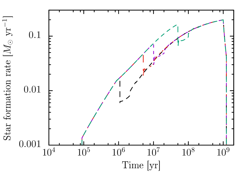
Figure 17: Simulation of the time evolution of the star formation rate (in the black hole field domination) of the starburst ring of NGC 6951. Different coloured dashed-lines indicate the feedback from supernovae explosions assuming different lifetimes for the responsible massive stars: $10^{6}$ years (black), $5\times 10^{6}$ years (red), $10^{7}$ years (violet) and  $5\times\leavevmode\nobreak\ 10^{7}$ years (green).

Table 3: Results from simulations: final values of the physical properties of NGC 6951.

Source of the gravitational field	Final ring stellar mass $[10^{8}$ $M_{\odot}]$	Ring radius [pc]	Final black hole mass $[10^{7}$ $M_{\odot}]$
Central Black hole	1.89	576	4.15
CND	1.79	573	4.38
Host galaxy	1.93	611	1.56

5 Discussion and conclusions

We have extended the co-evolution model of Wutschik et al. (2013) by implementing the turbulence-regulated star formation model of Krumholz & McKee (2005)(model KM05). We have additionally studied the time evolution of the Mach numbers as well as the AGN luminosity. The main results of this work are the following:

• The implementation of the KM05 model produces moderate fluctuations in the black hole mass accretion rates and star formation rates during the accretion phase rather than the strong fluctuations produced by the model EB10. The latter predicts over-accretion, i.e. the sonic speed becomes extremely large compared to the local sound speed which produces, in consequence, extreme Mach numbers up to $10^{4}$.

• We have studied the limiting cases of the total star formation rate under different assumptions for the gravitational field: dominated by the central black hole, the CND or the host galaxy. For each of these cases, our model is able to predict the growth of a SMBH from 10 million solar masses up to a few billions solar masses, with low (1 $M_{\odot}$ $\rm{yr}^{-1}$) and very large (1000 $M_{\odot}$ $\rm{yr}^{-1}$) mass supply rates respectively, in agreement with earlier work by Wutschik et al. (2013), Kawakatu & Wada (2009) and Volonteri et al. (2015). On the other hand, though that model EB10 produces an over-accretion, the final black hole masses are similar to the final values provided by model KM05 for gravity dominated by the CND. The final stellar masses generated by both models are also identical when compared at all field dominations.

• An increased mass supply rate enhances black hole accretion rates, star formation rate, disk radius final, black hole masses, final stellar masses as well as luminosities. However, we note that large mass supply rates dampen the level of turbulence and the competition of gas accretion during high accretion phases. This effect becomes more evident on the Mach number evolution when gravity is dominated by the central black hole. Large mass supply rates also significantly affect the disk radius; they lead to the growth of the inner and outer radii, from parsec scale to a few kilo-parsec. For instance, to produce an SMBH of a billion solar masses, our model predicts a final inner radius of 10 pc and outer radius of 500 pc. Our model shows that large mass supply rates have not only a significant impact on the final black hole mass or black hole accretion rates but also on the order of magnitude of AGN luminosities.

• Since our model considers high and low accretion phases during the evolution of the system, we have also assumed that the time evolution of the AGN luminosities follows similar phases accordingly. Adopting the slim disk approximation during the high accretion phase our model predicts super-Eddington luminosities, whereas sub-Eddington luminosities are found during the low accretion phase when the standard thin disk approximation is applied. The latter is reflected in the decrease of the luminosity after the end of the mass supply. However, afterwards it seems that the central black hole keeps accreting at very low rates of the order of $10^{-3}$ $M_{\odot}$ $\rm{yr}^{-1}$.

• As a result of the extended supply time and increased mass supply rate, our model is able to predict an upper limit on the AGN luminosity which is close to $10^{47}$ erg/s. AGN luminosities lower than $10^{47}$ erg/s are in agreement with Kawakatu & Wada (2008) and Kawakatu & Wada (2009). However, the upper limit is reached at a different time than the cosmological age of the observed AGN by Mortlock et al. (2011) and Pezzulli et al. (2016) (with references therein). However, we do not know when the mass supply started in the observed systems, and of course the real mass supply evolution may be more complex, i.e. time dependent. Despite this possible discrepancy with respect to time scales, our model succeeds in predicting the observed final black hole masses.

• We find that turbulence is a main driver of angular momentum redistribution (Balbus & Hawley, 1998);(Klessen & Hennebelle, 2010), and particularly high values of turbulence are found in the phase of high star formation rates and for the gravitational field dominated by the central black hole. We note that the turbulent velocity of gas becomes larger not only during the high accretion phase but also when the gas supply is depleted. While energy is injected by supernova explosions already at earlier stages of the accretion, the explosions occuring at the later stages are associated with the rise of the turbulent velocity due to a decreasing density, which is reflected in the peaks of the Mach number in the late evolutionary stages. We emphasize here that the timescale of supernova feedback sets the timescale for fluctuations in both the black hole accretion rate and star formation rate.

• Our model does not take into account any feedback from the AGN but if considered, it may indeed decrease the accretion rates and the jet emission may trigger star formation as investigated in MHD simulations by Gaibler et al. (2012).

• While our model does neither assume a specific structure of the galaxy nor take into account the interaction with the bar in NGC 6951, some quantities like the black hole mass and the stellar mass can still be reproduced. This suggests that these quantities may not strongly depend on the choice of the gravitational potential, though further investigations may be necessary in the future.