Value regions of univalent self-maps with two boundary fixed points

Abstract.

In this paper we find the exact value region $\mathcal{V}(z_{0},T)$ of the point evaluation functional $f\mapsto f(z_{0})$ over the class of all holomorphic injective self-maps $f:{\mathbb{D}}\to{\mathbb{D}}$ of the unit disk ${\mathbb{D}}$ having a boundary regular fixed point at $\sigma=-1$ with $f^{\prime}(-1)=e^{T}$ and the Denjoy – Wolff point at $\tau=1$.

1. Introduction

Since the seminal paper [11] by Cowen and Pommerenke, the study of holomorphic functions with finite angular derivative at prescribed boundary points has been an active field of research in Complex Analysis, see, e.g., [2, 3, 10, 15, 17, 31, 36], just to mention some works in the topic.

Given a holomorphic function $f$ in the unit disk ${\mathbb{D}}:=\{z:|z|<1\}$ and a point $\sigma\in{\partial{\mathbb{D}}}$ such that there exists finite angular limit $f(\sigma):=\angle\lim_{z\to\sigma}f(z)$, the angular derivative at $\sigma$ is $f^{\prime}(\sigma):=\angle\lim_{z\to\sigma}\big{(}f(z)-f(\sigma)\big{)}/(z-\sigma)$.

On the one hand, for univalent (i.e., holomorphic and injective) functions $f$, existence of the angular derivative $f^{\prime}(\sigma)$ different from $0$ and $\infty$ is closely related to the geometry of $f({\mathbb{D}})$ near $f(\sigma)$; moreover, if there exists $f^{\prime}(\sigma)\neq 0,\infty$, then the behaviour of $f$ at the boundary point $\sigma$ resembles conformality, see, e.g., [30, §§4.3, 11.4].

On the other hand, for the dynamics of a holomorphic (but not necessarily univalent) self-map $f:{\mathbb{D}}\to{\mathbb{D}}$, a crucial role is played by the points $\sigma\in{\partial{\mathbb{D}}}$ for which $f(\sigma)=\sigma$ (or, more generally, $f(\sigma)\in\partial{\mathbb{D}}$) and the angular derivative $f^{\prime}(\sigma)$ is finite, see, e.g., [ –, , , , , ]. Such points $\sigma$ are called boundary regular fixed points, see Section 2 for precise definitions and some basic theory. In particular, a classical result due to Wolff and Denjoy asserts that if $f\in{\sf Hol}({\mathbb{D}},{\mathbb{D}})$ has no fixed points in ${\mathbb{D}}$, then it possesses the so-called (boundary) Denjoy – Wolff point, i.e., a unique boundary regular fixed point $\tau$ such that $f^{\prime}(\tau)\leqslant 1$.

In this paper we study univalent self-maps $f:{\mathbb{D}}\to{\mathbb{D}}$ with a given boundary regular fixed point $\sigma\in{\partial{\mathbb{D}}}$ and the Denjoy – Wolff point $\tau\in{\partial{\mathbb{D}}}\setminus\{\sigma\}$. Using automorphisms of ${\mathbb{D}}$, we may suppose that $\tau=1$ and $\sigma=-1$. Our main result is the sharp value region of $f\mapsto f(z_{0})$ for all such self-maps of ${\mathbb{D}}$ with $f^{\prime}(-1)$ fixed. To give a detailed statement, fix $z_{0}\in{\mathbb{D}}$, $T>0$ and let $\zeta_{0}=x_{1}^{0}+ix_{2}^{0}:=\ell(z_{0})$, where

$$\ell\colon{\mathbb{D}}\to\mathbb{S};\quad z\mapsto\log\big{(}(1+z)/(1-z)\big{)}$$

is a conformal map of ${\mathbb{D}}$ onto the strip $\mathbb{S}:=\big{\{}\zeta\colon-\pi/2<\mathop{\mathsf{Im}}\zeta<\pi/2\big{\}}$. Define:

$$a_{\pm}(T):=\,e^{-T/2}\sin x_{2}^{0}\,\pm\,(1-e^{-T/2}),\quad R(a,T):=\log\frac{1-a}{1-a_{+}(T)}\,\,\log\frac{1+a}{1+a_{-}(T)},$$

$$V(\zeta_{0},T):=\Big{\{}x_{1}+ix_{2}\in\mathbb{S}\colon a_{-}(T)\leqslant\sin x_{2}\leqslant a_{+}(T),~{}\big{|}x_{1}-x_{1}^{0}-\tfrac{T}{2}\big{|}\leqslant\sqrt{R(\sin x_{2},T)}\,\Big{\}}.$$

Theorem 1.

Let $f\in{\sf Hol}({\mathbb{D}},{\mathbb{D}})\setminus\{{\sf id}_{\mathbb{D}}\}$ and $T>0$. Suppose that:

• $f$ is univalent in ${\mathbb{D}}$;

• the Denjoy – Wolff point of $f$ is $\tau=1$;

• $\sigma=-1$ is a boundary regular fixed point of $f$ and $f^{\prime}(-1)=e^{T}$.

Then

(1.1) $$f(z_{0})\in\mathcal{V}(z_{0},T):=\ell^{-1}\big{(}V(\ell(z_{0}),T)\big{)}\setminus\{z_{0}\}\quad\text{for any~{}$z_{0}\in{\mathbb{D}}$}.$$

This result is sharp, i.e., for any $w_{0}\in\mathcal{V}(z_{0},T)$ there exists $f\in{\sf Hol}({\mathbb{D}},{\mathbb{D}})\setminus\{{\sf id}_{\mathbb{D}}\}$ satisfying (i) – (iii) and such that ${f(z_{0})=w_{0}}$.

We can also characterize functions $f$ delivering boundary points of $\mathcal{V}(z_{0},T)$. In many extremal problems for univalent functions $f:{\mathbb{D}}\to{\mathbb{C}}$ normalized by $f(0)=f^{\prime}(1)-1=0$, the Koebe function $f_{0}(z):=z/(1-z)^{2}$ mapping ${\mathbb{D}}$ onto ${\mathbb{C}}\setminus(-\infty,\tfrac{1}{4}]$, and its rotations $f_{\theta}(z)=e^{i\theta}f_{0}(e^{-i\theta}z)$, $\theta\in{\mathbb{R}}$, are known to be extremal. For bounded univalent functions $f:{\mathbb{D}}\to{\mathbb{D}}$ normalized by $f(0)=0$, $f^{\prime}(0)>0$, the role of the Koebe function is played by the Pick functions $p_{\alpha}(z):=f_{0}^{-1}(\alpha f_{0}(z))$, $\alpha\in(0,1)$, mapping ${\mathbb{D}}$ onto ${\mathbb{D}}\setminus[-1,-r]$, $r=r(\alpha)\in(0,1)$. In our case, it would be natural to expect that some functions of the form $f=h_{1}\circ p_{\alpha}\circ h_{2}$, where $h_{1},h_{2}\in{\sf Aut}({\mathbb{D}})$, are extremal.

Theorem 2.

For any $w_{0}\in\partial\mathcal{V}(z_{0},T)\setminus\{z_{0}\}$, there exists a unique $f=f_{w_{0}}$ satisfying conditions (i) – (iii) in Theorem 1 and such that ${f_{w_{0}}(z_{0})=w_{0}}$. If $w_{0}=\ell^{-1}(\zeta_{0}+T)$, then $f_{w_{0}}$ is a hyperbolic automorphism of ${\mathbb{D}}$, namely $f_{w_{0}}(z)=\ell^{-1}(\ell(z)+T)$. Otherwise, $f_{w_{0}}$ is a conformal mapping of ${\mathbb{D}}$ onto ${\mathbb{D}}$ minus a slit along an analytic Jordan arc $\gamma$ orthogonal to $\partial{\mathbb{D}}$, with $f_{w_{0}}^{\prime}(1)=1$. Moreover, $f_{w_{0}}=h_{1}\circ p_{\alpha}\circ h_{2}$ for some $h_{1},h_{2}\in{\sf Aut}({\mathbb{D}})$ and $\alpha\in(0,1)$ if and only if $w_{0}=\ell^{-1}\big{(}x_{1}^{0}+\tfrac{T}{2}+i\arcsin a_{\pm}(T)\big{)}.$

Remark 1.1.

Note that $z_{0}$ is a boundary point of the value region $\mathcal{V}(z_{0},T)$, but does not belong to $\mathcal{V}(z_{0},T)$. The proof of the above theorem, given in Section 4, shows that $z_{0}$ would be included, and this would be the only modification of the value region, if we replaced the equality ${f^{\prime}(-1)=e^{T}}$ in condition (iii) of Theorem 1 by the inequality ${f^{\prime}(-1)\leqslant e^{T}}$ and removed the requirement $f\neq{\sf id}_{\mathbb{D}}$ assuming as a convention that ${\sf id}_{\mathbb{D}}$ satisfies (ii). Note also that under the conditions of Theorem 1 modified in this way, $f(z_{0})=z_{0}$ if and only if $f={\sf id}_{\mathbb{D}}$, see Remark 2.3.

If $f\in{\sf Hol}({\mathbb{D}},{\mathbb{D}})$ has boundary regular fixed points at $\pm 1$, then replacing $f$ by $h\circ f$, where $h$ is a suitable hyperbolic automorphism with the same boundary fixed points, we may suppose that $\tau=1$ is the Denjoy – Wolff point. In this way, as a corollary of Theorems 1 and 2 we easily deduce a sharp estimate for $f^{\prime}(-1)f^{\prime}(1)$, which was obtained earlier with the help of the extremal length method in [15, Section 4].

Corollary 1.

Let $z_{0}\in{\mathbb{D}}$ and let $f\in{\sf Hol}({\mathbb{D}},{\mathbb{D}})$ be a univalent function with boundary regular fixed points at $1$ and $-1$. Then

(1.2) $$\sqrt{f^{\prime}(-1)f^{\prime}(1)}\geqslant L\,\big{(}\sin\mathop{\mathsf{Im}}\ell(z_{0}),\,\sin\mathop{\mathsf{Im}}\ell(f(z_{0}))\big{)},\quad L(a,b):=\max\left\{\tfrac{1+a}{1+b},\tfrac{1-a}{1-b}\right\}.$$

Inequality (1.2) is sharp. The equality can occur only for hyperbolic automorphisms and functions of the form $f=h_{1}\circ p_{\alpha}\circ h_{2}$, $h_{1},h_{2}\in{\sf Aut}({\mathbb{D}})$, $\alpha\in(0,1)$.

Recently, the sharp value regions of $f\mapsto f(z_{0})$ have been determined for other classes of univalent self-maps [22, 33, 35]. The main instrument is the classical parametric representation of univalent functions, going back to the seminal work by Loewner [27]. In this paper, we use a new variant of Loewner’s parametric method, which is specific for functions satisfying conditions of Theorem 1. This variant of parametric representation was discovered quite recently, see [19, 20]. We discuss it in Section 3.

It is also worth mentioning that in [17], using another specific variant of the parametric representation, Goryainov obtained the sharp value region of $f\mapsto f^{\prime}(0)$ in the class of all univalent $f\in{\sf Hol}({\mathbb{D}},{\mathbb{D}})$, $f(0)=0$, having a boundary regular fixed point at $\sigma=1$ with a given value of $f^{\prime}(1)$.

To complete the Introduction, we recall another related result announced by Goryainov [18]. Dropping the univalence requirement, one can study holomorphic self-maps ${f:{\mathbb{D}}\to{\mathbb{D}}}$ satisfying conditions (ii) and (iii) in Theorem 1 by using relationships between boundary regular fixed points and the Alexandrov – Clark measures. In particular, according to [18], the value region $\mathcal{D}(0,T)$ of $f\mapsto f(0)$ over all such self-maps $f$ is the closed disk whose diameter is the segment $\big{[}0,\ell^{-1}(T)\big{]}$, with the boundary point $z_{0}=0$ excluded. Analyzing the functions delivering the boundary points of $\mathcal{D}(0,T)$, one can conclude that $\partial\mathcal{D}(0,T)~{}\bigcap~{}\partial\mathcal{V}(0,T)=\{0,\ell^{-1}(T)\}$.

2. Holomorphic self-maps of the unit disk

In this section we cite some basic theory of holomorphic self-maps of ${\mathbb{D}}$. More details can be found, e.g., in the monograph [1].

Let $f\in{\sf Hol}({\mathbb{D}},{\mathbb{D}})$ and $\sigma\in{\partial{\mathbb{D}}}$. According to the classical Julia – Wolff – Carathéodory Theorem, see, e.g., [1, Theorem 1.2.5, Proposition 1.2.6, Theorem 1.2.7], if

(2.1) $$\alpha_{f}(\sigma):=\liminf_{{\mathbb{D}}\ni z\to\sigma}\frac{1-|f(z)|}{1-|z|}<+\infty,$$

then

(2.2) $$\exists~{}\angle\lim_{z\to\sigma}f(z)=:f(\sigma)\in{\partial{\mathbb{D}}},\quad\exists~{}\angle\lim_{z\to\sigma}\frac{f(z)-f(\sigma)}{z-\sigma}=:f^{\prime}(\sigma)=\alpha_{f}(\sigma)\frac{f(\sigma)}{\sigma},~{}\hbox to0.0pt{$\displaystyle~{}\text{and}$\hss}$$

(2.3) $$\frac{|f(z)-f(\sigma)|^{2}}{1-|f(z)|^{2}}\leqslant|f^{\prime}(\sigma)|\,\frac{|z-\sigma|^{2}}{1-|z|^{2}}\qquad\text{for all}~{}z\in{\mathbb{D}},$$

with the equality sign if and only if $f\in{\sf Aut}({\mathbb{D}})$. Note that in its turn, existence of the limits in (2.2) satisfying $f(\sigma)\in{\partial{\mathbb{D}}}$ and $f^{\prime}(\sigma)\neq\infty$ immediately implies (2.1).

Definition 2.1.

Points $\sigma\in{\partial{\mathbb{D}}}$ satisfying (2.2) are referred to as regular contact points of $f$. If in addition to (2.2), $f(\sigma)=\sigma$, then $\sigma$ is said to be a regular fixed point of $f$. The number $f^{\prime}(\sigma)$ is called the angular derivative of $f$ at $\sigma$.

Among all fixed points (boundary and internal) of a self-map $f\neq{\sf id}_{\mathbb{D}}$, there is one point of special importance for dynamics. On the one hand, if $f(\tau)=\tau$ for some $\tau\in{\mathbb{D}}$, then by the Schwarz Lemma, $\tau$ is the only fixed point of $f$ in ${\mathbb{D}}$. If in addition, $f$ is not an elliptic automorphism, then $|f^{\prime}(\tau)|<1$ and hence the sequence of iterates $(f^{\circ n})$, $f^{\circ 1}:=f$, $f^{\circ(n+1)}:=f\circ f^{\circ n}$, converges (to the constant function equal) to $\tau$ locally uniformly in ${\mathbb{D}}$. On the other hand, if $f$ has no fixed points in ${\mathbb{D}}$, then by the Denjoy – Wolff Theorem, see, e.g. [1, Theorem 1.2.14, Corollary 1.2.16, Theorem 1.3.9], $f$ has a unique boundary regular fixed point $\tau\in{\partial{\mathbb{D}}}$ such that ${f^{\prime}(\tau)\leqslant 1}$ and moreover, $f^{\circ n}\to\tau$ locally uniformly in ${\mathbb{D}}$ as $n\to+\infty$.

Definition 2.2.

The point $\tau$ above is referred to as the Denjoy – Wolff point of $f$.

Remark 2.3.

Since the strict inequality holds in (2.3) unless ${f\in{\sf Aut}({\mathbb{D}})}$, a self-map $f$ can have a fixed point in ${\mathbb{D}}$ and a boundary regular fixed point $\sigma$ with $f^{\prime}(\sigma)\leqslant 1$ only if ${f={\sf id}_{\mathbb{D}}}$.

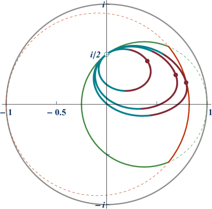
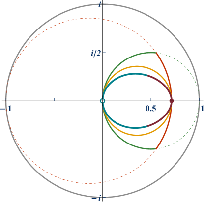
   ${\partial{\mathbb{D}}}$   $\scriptstyle\circ$$z_{0}$       ${\displaystyle\Gamma^{\hbox{$\scriptstyle\hskip 0.30873pt\raise 0.37973pt\hbox{$\scriptstyle-$}\hskip-0.1323pt$}\!}}$   $\scriptstyle\bullet$$\ell^{-1}(\ell(z_{0})+T)$      ${\displaystyle\Gamma^{\hbox{$\scriptstyle+$}\!}}$       $\partial D_{1}$       $\partial D_{2}$        $\partial\mathcal{D}(0,T)$

Figure 1. The value region $\mathcal{V}(z_{0},T)$ and the disks $D_{1}$, $D_{2}$ for $z_{0}:=i/2$, ${T\in\{\log 2,\log 4,\log 6\}}$ and for $z_{0}:=0$, $T:=\log 6$. The right picture also shows the disk $\mathcal{D}(0,T)$. Notation ${\displaystyle\Gamma^{\hbox{$\scriptstyle\pm$}\!}}$ is explained in Section 4.

Remark 2.4.

Let $f_{n}(z):=-\sigma H^{-1}\big{(}\alpha/H(z/\sigma)+\beta/(H(z/\sigma)+n)\big{)}$, where $n\in\mathbb{N}$, $\alpha,\beta>0$, and $H(z):=(1+z)/(1-z)$. Note that $f_{n}({\mathbb{D}})\subset{\mathbb{D}}$ for all $n\in\mathbb{N}$ and that $f_{n}(z)\longrightarrow f(z):=(z+c)/(1+\overline{c}z)$, $c:=\sigma(1-\alpha)/(1+\alpha)$, locally uniformly in ${\mathbb{D}}$ as $n\to+\infty$. Moreover, $f_{n}(\sigma)=f(\sigma)=\sigma$ and $f_{n}^{\prime}(\sigma)=\alpha+\beta$ for all $n\in\mathbb{N}$, but $f^{\prime}(\sigma)=\alpha$. This example shows that the map $f\mapsto f^{\prime}(\sigma)$ is not continuous. However, it turns out to be semicontinuous in the following sense. Suppose that $f_{n}(z)\to f(z)$ as $n\to+\infty$ and that $\sigma\in{\partial{\mathbb{D}}}$ is a boundary regular fixed point of $f_{n}\in{\sf Hol}({\mathbb{D}},{\mathbb{D}})$ for all $n\in\mathbb{N}$ with $\alpha:=\liminf_{n\to+\infty}f_{n}^{\prime}(\sigma)<+\infty$. Then passing in Julia’s inequality (2.3) applied for functions $f_{n}$ to the limit, we conclude that $f$ satisfies (2.3) with $|f^{\prime}(\sigma)|$ replaced by $\alpha$. It follows that ${\alpha_{f}(\sigma)\leqslant\alpha<+\infty}$. Therefore, either $f\equiv\sigma$ or $f\in{\sf Hol}({\mathbb{D}},{\mathbb{D}})$ and $\sigma$ is a regular boundary fixed point of $f$ with $f^{\prime}(\sigma)\leqslant\alpha$. As a consequence, the set of all $f\in{\sf Hol}({\mathbb{D}},{\mathbb{D}})$ sharing two different boundary regular fixed points $\sigma_{1}$ and $\sigma_{2}$ and satisfying $f^{\prime}(\sigma_{j})\leqslant\alpha_{j}<+\infty$, $j=1,2$, is compact.

According to inequality (2.3), the value region $\mathcal{V}(z_{0},T)$ in Theorem 1 lies in the intersection of two closed disks $D_{1},D_{2}\subset\hskip 0.24994pt\overline{\hskip-0.24994pt\vphantom{b}{\mathbb{D}}\hskip-1.00006pt}\hskip 1.00006pt$ whose boundaries pass through $z_{0}$ and $\tau=1$ and through $\ell^{-1}(\ell(z_{0})+T)$ and $\sigma=-1$, respectively. Comparison of $\mathcal{V}(z_{0},T)$ with $D_{1}\cap D_{2}$ is show in Figure 1. On the right picture, for which $z_{0}=0$, we also place the value range $\mathcal{D}(0,T)$ of $f\mapsto f(0)$ over all holomorphic but not necessary injective maps $f:{\mathbb{D}}\to{\mathbb{D}}$ satisfying conditions (ii) and (iii) in Theorem 1, see [18].

3. Parametric representation

Denote the class of all $f\in{\sf Hol}({\mathbb{D}},{\mathbb{D}})$ satisfying conditions (i) – (iii) in Theorem 1 by $\mathfrak{U}(T)$. The following theorem, proved in [20], gives a parametric representation for $\mathfrak{U}(T)$ in terms of a Loewner – Kufarev-type ODE.

Theorem 3 ([20, Corollary 1.2]).

The class $\mathfrak{U}(T)$ coincides with the set of all functions representable in the form $f(z)=w_{z}(T)$ for all $z\in{\mathbb{D}}$, where $w_{z}(t)$ is the unique solution to the initial value problem

(3.1) $$\frac{\mathrm{d}w_{z}}{\mathrm{d}t}=\tfrac{1}{4}(1-w_{z})^{2}(1+w_{z})q(w_{z},t),\quad t\in[0,T],\qquad w_{z}(0)=z,$$

with some function $q:{\mathbb{D}}\times[0,T]\to{\mathbb{C}}$ satisfying the following conditions:

• for every $z\in{\mathbb{D}}$, $q(z,\cdot)$ is measurable on $[0,T]$;

• for a.e. $t\in[0,T]$, $q(\cdot,t)$ has the following integral representation

  (3.2) $$q(z,t)=\int\limits_{{\partial{\mathbb{D}}}\setminus\{1\}}\!\!\frac{1-\kappa}{1+\kappa z}\,\,\mathrm{d}\nu_{t}(\kappa),$$

  where $\nu_{t}$ is a probability measure on ${\partial{\mathbb{D}}}\setminus\{1\}$.

Remark 3.1.

A related parametric representation for a class of univalent self-maps of a strip was considered in [13].

Remark 3.2.

In many cases, it is more convenient to deal with the the union $\mathfrak{U}^{\prime}(T):=\bigcup_{0\leqslant T^{\prime}\leqslant T}\mathfrak{U}(T^{\prime})$, where we define $\mathfrak{U}(0):=\{{\sf id}_{\mathbb{D}}\}$. Indeed, it is evident from the argument of Remark 2.4 that in contrast to $\mathfrak{U}(T)$, the class $\mathfrak{U}^{\prime}(T)$ is compact. Moreover, it is easy to see that Theorem 3 gives representation of $\mathfrak{U}^{\prime}(T)$ if all probability measures $\nu_{t}$ in (3.2) are replaced with all positive Borel measures $\nu_{t}$ satisfying

(3.3) $$\nu_{t}({\partial{\mathbb{D}}}\setminus\{1\})\,\in\,[0,1].$$

Note that the possibility of $\nu_{t}=0$ is not excluded.

Remark 3.3.

Obviously, the right-hand side of (3.1) can be written as $G(w_{z},t)$, where $G(z,t):=\tfrac{1}{4}(1-z)^{2}(1+z)q(z,t)$ with $q$ satisfying conditions (i) and (ii) in Theorem 3. By [19, Theorem 1], $G(\cdot,t)$ is an infinitesimal generator in ${\mathbb{D}}$ for each $t\in[0,T]$. For simplicity, extend $G$ to all $t\geqslant 0$ by setting $G(z,t)\equiv 0$ for any $t>T$. Then according to the general theory of Loewner – Kufarev-type equations, see [4, Sections  3–5], for any $s\geqslant 0$ and any $z\in{\mathbb{D}}$, the initial value problem $\mathrm{d}w/\mathrm{d}t=G(w,t)$, $t\geqslant s$, $w(s)=z,$ has a unique solution $w=w_{z,s}(t)$ defined for all $t\geqslant s$ and the functions $\varphi_{s,t}(z):=w_{z,s}(t)$, $z\in{\mathbb{D}}$, $t\geqslant s\geqslant 0$, form an evolution family, see [4, Definition  3.1].

Proposition 1.

Let $\vartheta:[0,T]\to(-\pi,\pi)\setminus\{0\}$, $T>0$, be a $C^{1}$-smooth function. Suppose that in the conditions of Theorem 3, $\mathrm{d}\nu_{t}(e^{i\theta})=\delta\big{(}\theta-\vartheta(t)\big{)}\,\mathrm{d}\theta$ for all ${t\in[0,T]}$, where $\delta$ stands for the Dirac delta function. Then $f$ maps ${\mathbb{D}}$ onto ${\mathbb{D}}\setminus\gamma$, where $\gamma$ is a slit in ${\mathbb{D}}$, i.e. $\gamma$ is the image of a homeomorphism $\gamma:[0,1]\mapsto\overline{\mathbb{D}}$ with $\gamma\big{(}[0,1)\big{)}\subset{\mathbb{D}}$ and $\gamma(1)\in{\partial{\mathbb{D}}}$.

Moreover:

• if $\vartheta$ is a real-analytic function on $[0,T]$, then $\gamma$ is a real-analytic Jordan arc orthogonal to ${\mathbb{D}}$;

• $\gamma$ is a circular arc or a straight line segment orthogonal to ${\partial{\mathbb{D}}}$ if and only if

  (3.4) $$\lambda(t):=i\frac{1+e^{i\vartheta(t)}}{1-e^{i\vartheta(t)}}=C_{1}e^{-t/2}\left(C_{2}e^{t/2}+\sqrt{C_{2}^{2}(e^{t}-1)+1}\right)^{3}$$

  for all  $t\in[0,T]$ and some constants $C_{1},C_{2}\in{\mathbb{R}}$, $C_{1}\neq 0$.

Proof.

In the conditions of the proposition, (3.1) takes the following form:

(3.5) $$\frac{\mathrm{d}w_{z}}{\mathrm{d}t}=\tfrac{1}{4}(1-w_{z})^{2}(1+w_{z})\frac{1-e^{i\vartheta(t)}}{1+e^{i\vartheta(t)}w_{z}},\quad t\in[0,T],\qquad w_{z}(0)=z.$$

The change of variables $\omega_{z}:=H(w_{z})$, where $H(w):=i(1+w)/(1-w)$ maps ${\mathbb{D}}$ conformally onto ${{\mathbb{H}}:=\{\omega\colon\mathop{\mathsf{Im}}\omega>0\}}$, transforms the above problem to

(3.6) $$\frac{\mathrm{d}\omega_{z}}{\mathrm{d}t}=\frac{\omega_{z}}{1-\lambda(t)\omega_{z}},\quad t\in[0,T],\qquad\omega_{z}(0)=H(z),$$

where $\lambda(t):=H(e^{i\vartheta(t)})$ for all $t\in[0,T]$. Making further change of variables

$$\hat{\omega}_{z}(t):=\omega_{z}(t)+\int_{0}^{t}\!\frac{\mathrm{d}s}{\lambda(s)},\qquad\xi(t):=\frac{1}{\lambda(t)}+\int_{0}^{t}\!\frac{\mathrm{d}s}{\lambda(s)},\qquad\tau=v(t):=\frac{1}{2}\int_{0}^{t}\!\frac{\mathrm{d}s}{\lambda(s)^{2}},$$

we obtain the chordal Loewner equation

(3.7) $$\frac{\mathrm{d}\hat{\omega}_{z}}{\mathrm{d}\tau}=\frac{2}{\xi-\hat{\omega}_{z}},\quad\tau\in[0,v(T)],\qquad\hat{\omega}_{z}(0)=H(z).$$

The geometry of solutions to (3.7) is well-studied, see, e.g., [25, 28, 34, 21, 37]; see also [23]. In particular, since the function $s\mapsto\xi(v^{-1}(s))$ is $C^{1}$-smooth, it follows that $z\mapsto\hat{\omega}_{z}(T)$ maps ${\mathbb{D}}$ onto ${\mathbb{H}}$ minus a slit along some Jordan arc $\gamma_{0}$. Taking into account that $w_{z}(T)=H^{-1}\big{(}\hat{\omega}_{z}(T)-C\big{)}$, where $C:=\int_{0}^{T}\!\lambda(t)^{-1}\,\mathrm{d}t$, this proves the first part of the proposition.

If $\vartheta$ is real-analytic, then $s\mapsto\xi(v^{-1}(s))$ is real-analytic on $[0,T]$ as well, and hence by [26, Theorem 1.4],  $\gamma_{0}$ is a real-analytic Jordan arc. Moreover, the argument of [26, Section 6.1] shows that in such a case, $\gamma_{0}$ is orthogonal to ${\mathbb{R}}$. This proves (i).

It remains to prove (ii). Suppose that $\gamma$ is a circular arc or a straight line segment orthogonal to ${\partial{\mathbb{D}}}$. Then we can find a linear-fractional transformation $H_{*}$ of ${\mathbb{D}}$ onto ${\mathbb{H}}$ such that $H_{*}(\gamma)=[0,i]$. Let $(\varphi_{s,t})$ be the evolution family associated with equation (3.5), see Remark 3.3. Note that $\varphi_{t,T}({\mathbb{D}})\supset\varphi_{t,T}(\varphi_{0,t}({\mathbb{D}}))=\varphi_{0,T}({\mathbb{D}})=f({\mathbb{D}})$ for any $t\in[0,T]$. It follows that the intersection of a sufficiently small neighbourhood of $H_{*}^{-1}(\infty)$ with $\partial\varphi_{t,T}({\mathbb{D}})$ is an open arc of ${\partial{\mathbb{D}}}$ containing $H_{*}^{-1}(\infty)$. Therefore, for each $t\in[0,T]$, there exists a unique $h_{t}\in{\sf Aut}({\mathbb{D}})$ such that $g_{t}:=H_{*}\circ\varphi_{t,T}\circ h_{t}\circ H_{*}^{-1}\in{\sf Hol}({\mathbb{H}},{\mathbb{H}})$ satisfies the Laurent expansion $g_{t}(z)=z-c(t)/z+\ldots$ at $\infty$ with some $c(t)\in{\mathbb{R}}$.

Denote $H_{t}:=H_{*}\circ h_{t}^{-1}$ for all $t\in[0,T]$. By construction, ${\mathbb{H}}\setminus[0,i]=g_{0}({\mathbb{H}})\subset g_{t}({\mathbb{H}})\subset g_{T}({\mathbb{H}})={\mathbb{H}}$ for all $t\in[0,T]$. Thanks to continuity of $\vartheta$, the function $t\mapsto c(t)$ is $C^{1}$-smooth. Therefore, according to the classical result [24] by Kufarev et al, see also [12], for any $z\in{\mathbb{D}}$, $\tilde{\omega}_{z}(t):=g_{t}^{-1}\circ g_{0}(H_{0}(z))$, $t\in[0,T]$, is the unique solution to the initial value problem $\mathrm{d}{\tilde{\omega}_{z}}/\mathrm{d}t=-c^{\prime}(t)/\tilde{\omega}_{z}$, $\tilde{\omega}_{z}(0)=H_{0}(z)\in{\mathbb{H}}$.

By construction, $\tilde{\omega}_{z}(t)=H_{t}(w_{z})$ for all $t\in[0,T]$ and all $z\in{\mathbb{D}}$. Comparing the differential equations for $\tilde{\omega}_{z}$ and $w_{z}$, one can conclude that for all $t\in[0,T]$,

(3.8) $$H_{t}(w):=\frac{\lambda(t)H(w)-1}{a(t)\big{(}\lambda(t)H(w)-1\big{)}+b(t)}$$

with real coefficients $a(t)$ and $b(t)$ satisfying

(3.9) $$\mathrm{d}a/\mathrm{d}t=a^{3}/b^{2},\quad\mathrm{d}b/\mathrm{d}t=-3a+b+3a^{2}/b,\qquad t\in[0,T],$$

and such that ${\lambda^{\prime}(t)/\lambda(t)=1-3a(t)/b(t)}$ and ${b(t)\lambda(t)>0}$ for all $t\in[0,T]$. System (3.9) can be solved by introducing a new unknown function $k(t):=a(t)/b(t)$. In this way, one can easily check that $\lambda$ must be of the form (3.4).

Conversely, if $\lambda$ is given by (3.4), then system (3.9) has a real-valued solution satisfying ${\lambda^{\prime}(t)/\lambda(t)=1-3a(t)/b(t)}$ and ${b(t)\lambda(t)>0}$ for all $t\in[0,T]$. It follows that for any $z\in{\mathbb{D}}$, the function $\tilde{\omega}_{z}(t):=H_{t}(w_{z}(t))$, where $H_{t}$ is given by (3.8), is a solution to $\mathrm{d}{\tilde{\omega}_{z}}/\mathrm{d}t=-1/\big{(}b(t)^{2}\,\tilde{\omega}_{z}\big{)}$, $t\in[0,T]$, $\tilde{\omega}_{z}(0)=H_{0}(z)\in{\mathbb{H}}$. Solving the latter initial value problem for $\tilde{\omega}_{z}$, we conclude that the image of the map ${{\mathbb{D}}\ni z\mapsto\tilde{\omega}_{z}(T)}$ is the domain ${\mathbb{H}}\setminus[0,i\sqrt{Q_{T}}\,]$, $Q_{T}:=\smash{2\int_{0}^{T}\!b(t)^{-2}\,\mathrm{d}t}$. Thus, $\gamma=H_{T}^{-1}\big{(}[0,i\sqrt{Q_{T}}\,]\big{)}$ is a circular arc or a straight line segment orthogonal to ${\partial{\mathbb{D}}}$. The proof is now complete. ∎

4. Proof of the main results

In this section we prove Theorems 1 and 2. Fix $T>0$. We start by considering the problem to determine the compact value region $\{f(z_{0})\colon f\in\mathfrak{U}^{\prime}(T)\}$. Thanks to Theorem 3 and Remark 3.2, it coincides with the reachable set $\{w_{z_{0}}(T)\}$ of the controllable system (3.1) in which the measure-valued control $t\mapsto\nu_{t}$ satisfies (3.3). The change of variables

$$\zeta=\ell(w),\quad\lambda=i\frac{1+\kappa}{1-\kappa},$$

reduces our problem to finding the reachable set $\Omega^{\prime}_{T}:=\{\zeta(T)\}$ for the following controllable system

(4.1) $$\frac{\mathrm{d}\zeta}{\mathrm{d}t}=\int_{\mathbb{R}}\frac{\mathrm{d}\mu_{t}(\lambda)}{1-i\lambda e^{\zeta}},\quad t\in[0,T];\qquad\zeta|_{t=0}=\zeta_{0}:=\ell(z_{0}),$$

where $\mu_{t}$’s are positive Borel measures on ${\mathbb{R}}$ with $\mu_{t}({\mathbb{R}})\leqslant 1$. By using the prime in the notation $\Omega^{\prime}_{T}$ we emphasize that this reachable set corresponds to the class $\mathfrak{U}^{\prime}(T)$.

Denote $x_{1}:=\mathop{\mathsf{Re}}\zeta$ and $x_{2}:=\mathop{\mathsf{Im}}\zeta$. Note that $x_{2}\in(-\frac{\pi}{2},\frac{\pi}{2})$. For any fixed $\zeta={x_{1}+ix_{2}\in\mathbb{S}}$, the range of the right-hand side in (4.1), regarded as a function of the measure $\mu_{t}$, is the disk

$$\left\{\omega\in{\mathbb{C}}\colon\left|\omega-\frac{e^{-ix_{2}}}{2\cos x_{2}}\right|\leqslant\frac{1}{2\cos x_{2}}\right\}.$$

Therefore, replacing the measure-valued control $t\mapsto\mu_{t}$ with the complex-valued control

$$u(t):=2e^{ix_{2}}\cos x_{2}\int_{\mathbb{R}}\frac{\mathrm{d}\mu_{t}(\lambda)}{1-i\lambda e^{x_{1}+ix_{2}}},$$

we can rewrite (4.1) in the following form

(4.2) $$\frac{\mathrm{d}x_{1}}{\mathrm{d}t} =\mathop{\mathsf{Re}}\frac{u(t)e^{-ix_{2}}}{2\cos x_{2}}=\frac{1}{2}\mathop{\mathsf{Re}}u(t)+\frac{\mathop{\mathrm{tg}}x_{2}}{2}\mathop{\mathsf{Im}}u(t), x_{1}(0)=x_{1}^{0}:=\mathop{\mathsf{Re}}\zeta_{0},$$

(4.3) $$\frac{\mathrm{d}x_{2}}{\mathrm{d}t} =\mathop{\mathsf{Im}}\frac{u(t)e^{-ix_{2}}}{2\cos x_{2}}=\frac{1}{2}\mathop{\mathsf{Im}}u(t)-\frac{\mathop{\mathrm{tg}}x_{2}}{2}\mathop{\mathsf{Re}}u(t), x_{2}(0)=x_{2}^{0}:=\mathop{\mathsf{Re}}\zeta_{0},$$

where $u:[0,T]\to U:=\{u\colon|u-1|\leqslant 1\}$ is an arbitrary measurable function.

Introduce the Hamilton function

$${\mathcal{H}}(x_{1},x_{2},\Psi_{1},\Psi_{2},u):=\Psi_{1}\mathop{\mathsf{Re}}\frac{ue^{-ix_{2}}}{2\cos x_{2}}+\Psi_{2}\mathop{\mathsf{Im}}\frac{ue^{-ix_{2}}}{2\cos x_{2}}=\mathop{\mathsf{Re}}\frac{ue^{-ix_{2}}(\Psi_{1}-i\Psi_{2})}{2\cos x_{2}},$$

where $\Psi_{1}$, $\Psi_{2}$ satisfy the adjoint system of ODEs

(4.4) $$\frac{\mathrm{d}\Psi_{1}}{\mathrm{d}t}=-\frac{\partial{\mathcal{H}}}{\partial x_{1}}=0,\qquad\frac{\mathrm{d}\Psi_{2}}{\mathrm{d}t}=-\frac{\partial{\mathcal{H}}}{\partial x_{2}}=-\mathop{\mathsf{Im}}\frac{u(t)(\Psi_{1}-i\Psi_{2})}{2\cos^{2}x_{2}}.$$

Boundary points of the reachable set $\Omega^{\prime}_{T}$, forming a dense subset of $\partial\Omega^{\prime}_{T}$, are generated by the driving functions $u^{*}$ satisfying the necessary optimal condition in the form of Pontryagin’s maximum principle,

(4.5) $$\max_{u\in U}{\mathcal{H}}\big{(}x_{1}(t),x_{2}(t),\Psi_{1}(t),\Psi_{2}(t),u\big{)}={\mathcal{H}}\big{(}x_{1}(t),x_{2}(t),\Psi_{1}(t),\Psi_{2}(t),u^{*}(t)\big{)}$$

for all $t\in[0,T]$, see, e.g., [32]. Trajectories $(x_{1}(t),x_{2}(t))$ in (4.5) are optimal in the reachable set problem, and $(\Psi_{1}(t),\Psi_{2}(t))$ satisfy the adjoint system (4.4) with the optimal trajectories. In particular, $(\Psi_{1}(t),\Psi_{2}(t))$ does not vanish, and hence the maximum in (4.5) is attained at the unique point $u^{*}=1+e^{i(x_{2}+\varphi)}$, where $\varphi:=\arg(\Psi_{1}+i\Psi_{2})$. Therefore, from (4.2) – (4.4) for the optimal trajectories we obtain

(4.6) $$\frac{\mathrm{d}x_{1}}{\mathrm{d}t} =\frac{\cos\varphi+\cos x_{2}}{2\cos x_{2}}, x_{1}(0)=x_{1}^{0},$$

(4.7) $$\frac{\mathrm{d}x_{2}}{\mathrm{d}t} =\frac{\sin\varphi-\sin x_{2}}{2\cos x_{2}}, x_{2}(0)=x_{2}^{0},$$

(4.8) $$\frac{\mathrm{d}\Psi_{1}}{\mathrm{d}t} =0,$$

(4.9) $$\frac{\mathrm{d}\Psi_{2}}{\mathrm{d}t} =\frac{\sin\varphi-\sin x_{2}}{2\cos^{2}x_{2}}\,\big{|}\Psi_{1}-i\Psi_{2}\big{|}.$$

System (4.6) – (4.9) is invariant w.r.t. multiplication of $(\Psi_{1},\Psi_{2})$ by a positive constant. Therefore, we may assume that either $\Psi_{1}\equiv 0$, or $\Psi_{1}\equiv 1$, or $\Psi_{1}\equiv-1$.

If $\Psi_{1}\equiv 0$, then $\varphi=\pm\pi/2$ and we easily get that for all $t\geqslant 0$,

(4.10) $$x_{1}(t)=x_{1}(0)+t/2,\quad\sin x_{2}(t)=a_{\pm}(t):=e^{-t/2}\sin x_{2}(0)\pm(1-e^{-t/2}).$$

Now let $\Psi_{1}\equiv 1$. Then $\varphi\in(-\pi/2,\pi/2)$ and equation (4.9) takes the following form

(4.11) $$\frac{\mathrm{d}\varphi}{\mathrm{d}t}=\frac{\sin\varphi-\sin x_{2}}{2\cos^{2}x_{2}}\cos\varphi=\frac{\cos\mathrlap{\varphi}\hphantom{x_{2}}}{\cos x_{2}}\frac{\mathrm{d}x_{2}}{\mathrm{d}t}.$$

System (4.6), (4.11) admits the first integral

$$I(x_{2},\varphi):=\frac{1-\sin\varphi}{1+\sin\varphi}\,\,\frac{1+\sin x_{2}}{1-\sin x_{2}}\,>\,0,$$

and as a result it can be integrated in quadratures. Namely, if $C:=I\big{(}x_{2}(0),\varphi(0)\big{)}\neq 1$, we obtain the following identities

(4.12) $$B_{1}(t)-CB_{2}(t)=(C-1)t/2,$$

(4.13) $$x_{1}(t)-x_{1}(0)=\mathrlap{\frac{B_{1}(t)-\sqrt{C}B_{2}(t)}{\sqrt{C}-1},}$$

$$\quad\qquad\qquad\text{where}\quad B_{1}(t):=\log\frac{1-\sin x_{2}(t)}{1-\sin x_{2}(0)},\quad B_{2}(t):=\log\frac{1+\sin x_{2}(t)}{1+\sin x_{2}(0)}.$$

Excluding $C$ from (4.12), (4.13) and setting $t:=T$ gives

(4.14) $$x_{1}(T)=x_{1}(0)+\frac{1}{2}\Big{(}T+\sqrt{\big{(}T+2B_{1}(T)\big{)}\big{(}T+2B_{2}(T)\big{)}}\Big{)}\\ =x_{1}(0)+\frac{T}{2}+\sqrt{R\big{(}\sin x_{2}(T),T\big{)}},$$

where we took into account that according to (4.12),

$$\frac{\mathrm{d}}{\mathrm{d}t}\Big{(}t+2B_{1}(t)\Big{)}=\frac{2C}{1+\sin x_{2}(t)+C\big{(}1-\sin x_{2}(t)\big{)}}>0$$

and therefore, $T+2B_{1}(T)>0$.

For $C=1$, we have $\varphi(t)=x_{2}(t)$ and hence $\mathrm{d}\varphi/\mathrm{d}t=\mathrm{d}x_{2}/\mathrm{d}t=0$, $\mathrm{d}x_{1}/\mathrm{d}t=1$. Therefore, if $C=1$, then (4.12) and (4.14) hold as well.

Since $C>0$, from (4.12) we obtain that $x_{2}(T)\in J(T):=\big{(}\arcsin a_{-}(T),\arcsin a_{+}(T)\big{)}$. On the other hand, for any $x\in J(T)$ there exists a unique $C=C(x)>0$ that verifies (4.12) with $T$ and $x$ substituted for $t$ and $x_{2}(t)$, respectively. Solving $I(x_{2}(0),\varphi(0))=C(x)$ provides us with the initial condition in equation (4.11) for which $x_{2}(T)=x$.

Investigating the case $\Psi_{1}\equiv-1$ in a similar way, we conclude that $\partial\Omega^{\prime}_{T}$ is the union of the two Jordan arcs

$${\displaystyle\Gamma^{\hbox{$\scriptstyle\pm$}\!}}(T):=\Big{\{}x_{1}+ix_{2}\in\mathbb{S}\colon a_{-}(T)\leqslant\sin x_{2}\leqslant a_{+}(T),~{}x_{1}=x_{1}^{0}+\tfrac{T}{2}\pm\sqrt{R(\sin x_{2},T)}\,\Big{\}},$$

which do not intersect except for the common end-points $\omega^{\pm}:=x_{1}^{0}+T/2+i\arcsin a_{\pm}(T)$, delivered by solutions (4.10). Taking into account that by the very definition, $\mathfrak{U}^{\prime}(T^{\prime})\subset\mathfrak{U}^{\prime}(T)$ for any $T^{\prime}\in[0,T]$, it follows that $\Omega^{\prime}_{T}=V(\zeta_{0},T)$.

The next step in the proof is to pass from the class $\mathfrak{U}^{\prime}(T)$ to the class $\mathfrak{U}(T)$. In the problem of finding the value region of the functional $f\mapsto f(z_{0})$, this is equivalent to replacing the range $U$ of the admissible controls $u$ in (4.2) – (4.3) by $U\setminus\{0\}$. Denote by $\Omega_{T}$ the corresponding reachable set. By re-scaling the time, the problem to find $\Omega_{T^{\prime}}$, $T^{\prime}\in(0,T)$, can be restated as the reachable set problem at the same time $T$ and for the same controllable system, but with the value range of admissible controls restricted to $\alpha\big{(}U\setminus\{0\}\big{)}$, $\alpha:=T^{\prime}/T$. Note also that ${\displaystyle\Gamma^{\hbox{$\scriptstyle+$}\!}}(T)\cup{\displaystyle\Gamma^{\hbox{$\scriptstyle\hskip 0.34303pt\raise 0.42192pt\hbox{$\scriptstyle-$}\hskip-0.14699pt$}\!}}(T)\setminus\{\zeta_{0}\}\subset\Omega_{T}$ for any $T>0$. Since $\alpha\big{(}U\setminus\{0\}\big{)}\subset U\setminus\{0\}$ for any $\alpha\in(0,1)$, it follows that

$${\displaystyle\Gamma^{\hbox{$\scriptstyle+$}\!}}(T^{\prime})\cup{\displaystyle\Gamma^{\hbox{$\scriptstyle\hskip 0.34303pt\raise 0.42192pt\hbox{$\scriptstyle-$}\hskip-0.14699pt$}\!}}(T^{\prime})\setminus\{\zeta_{0}\}\subset\Omega_{T^{\prime}}\subset\Omega_{T}\quad\text{for any~{}$T\in(0,T]$}.$$

Thus $\Omega_{T}=V(\zeta_{0},T)\setminus\{\zeta_{0}\}$, which completes the proof of Theorem 1.

To prove Theorem 2, we have to identify the functions delivering the boundary points of $\mathcal{V}(z_{0},T)$. They correspond to the controls $u^{*}$ satisfying Pontryagin’s maximum principle (4.5). It is easy to see from the above argument that every point $\omega\in\partial\Omega^{\prime}_{T}\setminus\{\zeta_{0}\}$ corresponds to a unique control, which is $C^{1}$-smooth and takes values on $\partial U\setminus\{0\}$. It follows that the corresponding measures $\mu_{t}$ in (4.1) and the measures $\nu_{t}$ in the Loewner-type representation (3.1), (3.2) are also unique. They are probability measures concentrated at one point that moves smoothly with $t$. Namely, $\mathrm{d}\mu_{t}(\lambda)=\delta\big{(}\lambda-\lambda^{*}(t)\big{)}\,\mathrm{d}\lambda$, where

(4.15) $$\lambda^{*}(t):=\frac{1-2\cos x_{2}(t)/\big{(}e^{-ix_{2}(t)}+e^{i\varphi(t)}\big{)}}{ie^{x_{1}(t)+ix_{2}(t)}}=e^{-x_{1}(t)}\,\frac{~{}\raise 2.15277pt\hbox{$\sin\tfrac{\varphi(t)-x_{2}(t)}{2}$}~{}}{\lower 3.22916pt\hbox{$\cos\tfrac{\varphi(t)+x_{2}(t)}{2}$}\,}.$$

The point $\omega=\omega_{0}:=\zeta_{0}+T\in{\displaystyle\Gamma^{\hbox{$\scriptstyle+$}\!}}$ corresponds to $C=1$, in which case $\varphi(t)=x_{2}(t)$ for all $t\in[0,T]$ and hence $\lambda^{*}(t)\equiv 0$. Therefore, from (4.1) we see that the unique $f\in\mathfrak{U}(T)$ delivering the boundary point $\ell^{-1}(\omega_{0})$ of $\mathcal{V}(z_{0},T)$ is the hyperbolic automorphism

$$f(z)=\frac{z+c(T)}{1+c(T)z},\quad c(T):=\frac{e^{T}-1}{e^{T}+1},\quad\text{for all $z\in{\mathbb{D}}$}.$$

For the common end-points $\omega^{\pm}$ of ${\displaystyle\Gamma^{\hbox{$\scriptstyle+$}\!}}$ and ${\displaystyle\Gamma^{\hbox{$\scriptstyle\hskip 0.34303pt\raise 0.42192pt\hbox{$\scriptstyle-$}\hskip-0.14699pt$}\!}}$, which correspond to $\varphi=\pm\pi/2$, formula (4.15) simplifies to $\lambda^{*}(t)=\pm e^{-x_{1}(t)}$. In view of $\eqref{EQ_special-solutions}$, the latter expression coincides with $\lambda(t)$ given by (3.4) if we set $C_{1}:=\pm e^{-x_{1}^{0}}$ and $C_{2}:=0$. Taking into account the correspondence between $\mu_{t}$ and $\nu_{t}$ and applying Proposition 1, we conclude that the unique functions $f\in\mathfrak{U}(T)$ delivering the points $\ell^{-1}(\omega^{\pm})$ map ${\mathbb{D}}$ onto ${\mathbb{D}}$ minus a slit along a circular arc or a segment of a straight line orthogonal to ${\partial{\mathbb{D}}}$.

It remains to compare $\lambda^{*}(t)$ given by (4.15) with $\lambda(t)$ given by (3.4) for the case $\omega\in\partial\Omega_{T}\setminus\{\zeta_{0},\omega_{0},\omega^{+},\omega^{-}\}$. Suppose $\omega\in{\displaystyle\Gamma^{\hbox{$\scriptstyle+$}\!}}\setminus\{\omega_{0},\omega^{+},\omega^{-}\}$. Using equations (4.6), (4.7), (4.11) and taking into account the first integral $I(x_{2},\varphi)=C$, we find that

$$\Big{(}\,1\,+\,2\,\frac{\mathrm{d}}{\mathrm{d}t}\log\lambda^{*}(t)\,\Big{)}^{2}=\left(\frac{\,\cos\hbox to0.0pt{$\displaystyle\varphi(t)$\hss}\hphantom{x_{2}(t)}}{\,\cos x_{2}(t)}\right)^{2}=\frac{C\big{(}1-a^{2}\big{)}}{\big{(}(1+C)a+(1-C)a^{2}\big{)}^{2}},\quad a:=\sin x_{2}(t),$$

while $\big{(}1+2({\mathrm{d}}/{\mathrm{d}t})\log\lambda(t)\big{)}^{2}=9C_{2}^{2}\,e^{t}/\big{(}1+C_{2}^{2}(e^{t}-1)\big{)}$. However, according to (4.12), $e^{t}$ cannot be expressed as a rational function of $\sin x_{2}(t)$. This shows that $\lambda^{*}$ is not of the form (3.4) and hence, by Proposition 1, the unique function $f\in\mathfrak{U}(T)$ that delivers the boundary point $\ell^{-1}(\omega)$ maps ${\mathbb{D}}$ onto ${\mathbb{D}}$ minus a slit along a real-analytic arc $\gamma$ orthogonal to ${\partial{\mathbb{D}}}$ but different from a circular arc or a segment of a straight line. A similar argument applied to the case $\omega\in{\displaystyle\Gamma^{\hbox{$\scriptstyle\hskip 0.34303pt\raise 0.42192pt\hbox{$\scriptstyle-$}\hskip-0.14699pt$}\!}}\setminus\{\zeta_{0},\omega^{+},\omega^{-}\}$ completes the proof of Theorem 2.∎

References

• [1] M. Abate, Iteration theory of holomorphic maps on taut manifolds, Research and Lecture Notes in Mathematics. Complex Analysis and Geometry, Mediterranean, Rende, 1989. MR1098711
• [2] J. M. Anderson and A. Vasil’ev, Lower Schwarz-Pick estimates and angular derivatives, Ann. Acad. Sci. Fenn. Math. 33 (2008) No. 1, 101–110. MR2386840
• [3] V. Bolotnikov, M. Elin, D. Shoikhet, Inequalities for angular derivatives and boundary interpolation, Anal. Math. Phys. 3 (2013) No. 1, 63–96. MR3015631
• [4] F. Bracci, M. Contreras, S. Díaz-Madrigal, Evolution Families and the Loewner Equation I: the unit disc. J. Reine Angew. Math. (Crelle’s Journal), 672 (2012), 1–37. MR2995431
• [5] F. Bracci, M. D. Contreras, S. Díaz-Madrigal, and P. Gumenyuk, Boundary regular fixed points in Loewner theory, Ann. Mat. Pura Appl. (4) 194 (2015) No. 1, 221–245. MR3303013
• [6] F. Bracci and P. Gumenyuk, Contact points and fractional singularities for semigroups of holomorphic self-maps of the unit disc, J. Anal. Math. 130 (2016) No. 1, 185–217. MR3574653
• [7] M. D. Contreras and S. Díaz-Madrigal, Analytic flows on the unit disk: angular derivatives and boundary fixed points, Pacific J. Math. 222 (2005), 253–286. MR2225072
• [8] M. D. Contreras, S. Díaz-Madrigal and C. Pommerenke, Fixed points and boundary behaviour of the Koenigs function, Ann. Acad. Sci. Fenn. Math. 29 (2004) No. 2, 471–488. MR2097244
• [9] by same author, On boundary critical points for semigroups of analytic functions, Math. Scand. 98 (2006) No. 1, 125–142. MR2221548
• [10] M. D. Contreras, S. Díaz-Madrigal, A. Vasil’ev, Digons and angular derivatives of analytic self-maps of the unit disk, Complex Var. Elliptic Equ. 52 (2007) No. 8, 685-691. MR2346746
• [11] C. C. Cowen and C. Pommerenke, Inequalities for the angular derivative of an analytic function in the unit disk, J. London Math. Soc. (2) 26 (1982) No. 2, 271–289. MR0675170
• [12] A. del Monaco and P. Gumenyuk, Chordal Loewner equation, in Complex analysis and dynamical systems VI. Part 2, 63–77, Contemp. Math., 667, Israel Math. Conf. Proc., Amer. Math. Soc., Providence, RI, 2016. MR3511252
• [13] D. A. Dubovikov, An analog of the Löwner equation for mappings of strips, Izv. Vyssh. Uchebn. Zaved. Mat. 2007, no. 8, 77–80 (Russian); translation in Russian Math. (Iz. VUZ) 51 (2007), no. 8, 74–77. MR2396110
• [14] M. Elin, V. Goryainov, S. Reich, D. Shoikhet, Fractional iteration and functional equations for functions analytic in the unit disk, Comput. Methods Funct. Theory 2 (2002) No. 2, [On table of contents: 2004]. MR2038126
• [15] A. Frolova, M. Levenshtein, D. Shoikhet, A. Vasil’ev, Boundary distortion estimates for holomorphic maps, Complex Anal. Oper. Theory 8 (2014) No. 5, 1129–1149. MR3208806
• [16] V. V. Goryainov, Fractional iterates of functions that are analytic in the unit disk with given fixed points Mat. Sb. 182 (1991), no. 9, 1281–1299 (Russian); translation in Math. USSR-Sb. 74 (1993) No. 1, 29–46. MR1133569
• [17] by same author, Evolution families of conformal mappings with fixed points and the Löwner-Kufarev equation, Mat. Sb. 206 (2015), no. 1, 39–68; translation in Sb. Math. 206 (2015) No. 1-2, 33-60. MR3354961
• [18] by same author, Holomorphic self-maps of the unit disc with two fixed points. Presentation at XXV St. Petersburg Summer Meeting in Mathematical Analysis Tribute to Victor Havin (1933–2015), June 25–30, 2016. Available at http://gauss40.pdmi.ras.ru/ma25/index.php?page=presentations
• [19] V. V. Goryainov, O. S. Kudryavtseva, One-parameter semigroups of analytic functions, fixed points and the Koenigs function, Mat. Sb. 202 (2011) No. 7, 43–74 (Russian); translation in Sb. Math., 202 (2011) No. 7-8, 971–1000. MR2857793
• [20] P. Gumenyuk, Parametric representation of univalent functions with boundary regular fixed points. Accepted in Constr. Approx., 2017. Available at ArXiv:1603.04043.
• [21] G. Ivanov, D. Prokhorov, A. Vasil ev, Non-slit and singular solutions to the Löwner equation, Bull. Sci. Math. 136 (2012) No. 3, 328–341. MR2914952
• [22] J. Koch and S. Schleißinger, Value ranges of univalent self-mappings of the unit disc, J. Math. Anal. Appl. 433 (2016) No. 2, 1772–1789. MR3398791
• [23] P. P. Kufarev, On integrals of simplest differential equation with moving pole singularity in the righ-thand side (Russian), Tomsk. Gos. Univ. Uchyon. Zapiski 1 (1946), 35–48.
• [24] P. P. Kufarev, V. V. Sobolev, and L. V. Sporyševa, A certain method of investigation of extremal problems for functions that are univalent in the half-plane (Russian), Trudy Tomsk. Gos. Univ. Ser. Meh.-Mat. 200 (1968), 142–164. MR0257336
• [25] J. Lind, A sharp condition for the Loewner equation to generate slits, Ann. Acad. Sci. Fenn. Math. 30 (2005), 143–158. MR2140303
• [26] J. Lind and H. Tran, Regularity of Loewner curves, Indiana Univ. Math. J. 65 (2016) No. 5, 1675–1712. MR3571443
• [27] K. Löwner, Untersuchungen über schlichte konforme Abbildungen des Einheitskreises, Math. Ann. 89 (1923), 103–121. MR1512136
• [28] D. E. Marshall, S. Rohde, The Loewner differential equation and slit mappings, J. Amer. Math. Soc. 18 (2005), 763–778. MR2163382
• [29] P. Poggi-Corradini, Canonical conjugations at fixed points other than the Denjoy-Wolff point, Ann. Acad. Sci. Fenn. Math. 25 (2000) No. 2, 487–499. MR1762433
• [30] Ch. Pommerenke, Boundary behaviour of conformal mappings. Springer-Verlag, 1992. MR0623475
• [31] C. Pommerenke and A. Vasil’ev, Angular derivatives of bounded univalent functions and extremal partitions of the unit disk, Pacific J. Math. 206 (2002) No. 2, 425–450. MR1926785
• [32] L. S. Pontryagin, V. G. Boltyanskii, R. V. Gamkrelidze, E. F. Mishchenko, The mathematical theory of optimal processes (Russian), Gosudarstv. Izdat. Fiz.-Mat. Lit., Moscow, 1961. MR0166036; translations to English: MR0186436, MR0166037.
• [33] D. Prokhorov and K. Samsonova, Value range of solutions to the chordal Loewner equation, J. Math. Anal. Appl. 428 (2015) No. 2. MR3334955
• [34] D. Prokhorov, A. Vasil ev, Singular and tangent slit solutions to the Löwner equation, in Analysis and Mathematical Physics, 455–463. Trends in Mathematics. Birkhäuser Verlag, 2009. MR2724626
• [35] O. Roth and S. Schleißinger, Rogosinski’s lemma for univalent functions, hyperbolic Archimedean spirals and the Loewner equation, Bull. Lond. Math. Soc. 46 (2014) No. 5. MR3262210
• [36] A. Vasil’ev, On distortion under bounded univalent functions with the angular derivative fixed, Complex Var. Theory Appl. 47 (2002) No. 2, 131-147. MR1892514
• [37] C. Wong, Smoothness of Loewner slits. Trans. Am. Math. Soc. 366 (2014) No. 3, 1475–1496. MR3145739