Replicable Parallel Branch and Bound Search

Abstract

Combinatorial branch and bound searches are a common technique for solving global optimisation and decision problems. Their performance often depends on good search order heuristics, refined over decades of algorithms research. Parallel search necessarily deviates from the sequential search order, sometimes dramatically and unpredictably, e.g. by distributing work at random. This can disrupt effective search order heuristics and lead to unexpected and highly variable parallel performance. The variability makes it hard to reason about the parallel performance of combinatorial searches.

This paper presents a generic parallel branch and bound skeleton, implemented in Haskell, with replicable parallel performance. The skeleton aims to preserve the search order heuristic by distributing work in an ordered fashion, closely following the sequential search order. We demonstrate the generality of the approach by applying the skeleton to 40 instances of three combinatorial problems: Maximum Clique, 0/1 Knapsack and Travelling Salesperson. The overheads of our Haskell skeleton are reasonable: giving slowdown factors of between 1.9 and 6.2 compared with a class-leading, dedicated, and highly optimised C++ Maximum Clique solver. We demonstrate scaling up to 200 cores of a Beowulf cluster, achieving speedups of 100x for several Maximum Clique instances. We demonstrate low variance of parallel performance across all instances of the three combinatorial problems and at all scales up to 200 cores, with median Relative Standard Deviation (RSD) below 2%. Parallel solvers that do not follow the sequential search order exhibit far higher variance, with median RSD exceeding 85% for Knapsack.

1 Introduction

Branch and bound backtracking searches are a widely used class of algorithms. They are often applied to solve a range of NP-hard optimisation problems such as integer and non-linear programming problems; important applications include frequency planning in cellular networks and resource scheduling, e.g. assigning deliveries to routes [1].

Branch and bound systematically explores a search tree by sub-dividing the search space and branching recursively into each sub-space. The advantage of branch and bound over exhaustive enumeration stems from the way branch and bound prunes branches that cannot better the incumbent, i.e. the current best solution, potentially drastically reducing the number of branches to be explored.

The effectiveness of pruning depends on two factors: 1) the accuracy of the problem-specific heuristic to compute bounds 2) the value of optimal solutions in each branch, and on the quality of the incumbent; the closer to optimal the incumbent, the more can be pruned. As a result, branch and bound is sensitive to search order, i.e. to the order in which branches are explored.

A good search order can improve the performance of branch and bound dramatically by finding a good incumbent early on, and highly optimised sequential algorithms following the branch and bound paradigm often rely on very specific orders for performance.

Branch and bound algorithms are hard to parallelise for a number of reasons. Firstly, while branching creates opportunities for speculative parallelism where multiple workers i.e threads/processors search particular branches in parallel, pruning counteracts this, limiting potential parallelism. Secondly, parallel pruning requires processors sharing access to the incumbent, which limits scalability. Thirdly, parallel exploration of irregularly shaped search trees generates unpredictable numbers of parallel tasks, of highly variable duration, posing challenges for task scheduling. Finally, and most importantly, parallel exploration alters the search order, potentially impacting the effectiveness of pruning.

As a result of the last point in particular, parallel branch and bound searches can exhibit unusual performance characteristics. For instance, slowdowns can arise when the sequential search finds an optimal incumbent quickly but the parallel search delays exploring the optimal branch. Alternately, super-linear speedups are possible in case the parallel search happens on an optimal branch that the sequential search does not explore until much later. In short, the perturbation of the search order caused by adding processors makes it impossible to predict parallel performance.

These unusual performance characteristics make reproducible algorithmic research into combinatorial search difficult: was it the new heuristic that improved performance, or were we just lucky with the search ordering in this instance? As the instances we wish to tackle become larger, parallelism is becoming central to algorithmic research, and it is essential to be able to reason about parallel performance.

This paper aims to develop a generic parallel branch and bound search for distributed memory architectures (clusters). Crucially, the objective is predictable parallel performance, and the key to achieving this is careful control of the parallel search order.

The paper starts by illustrating performance anomalies with parallel branch and bound by using a Maximum Clique graph search. The paper then makes the following research contributions:

• To address search order related performance anomalies, Section 2 postulates three parallel search properties for replicable performance as follows.

  Sequential Bound:

  Parallel runtime is never higher than sequential (one worker) runtime.

  Non-increasing Runtimes:

  Parallel runtime does not increase as the number of workers increases.

  Repeatability:

  Parallel runtimes of repeated searches on the same parallel configuration have low variance.

• We define a novel formal model for general parallel branch and bound backtracking search problems (BBM) that specifies both search order and parallel reduction (Section 3). We show the generality of BBM by using it to define three different benchmarks with a range of application areas: Maximum Clique (Section 3), 0/1 Knapsack (Appendix B) and Travelling Salesperson (Appendix D).

• We define a new Generic Branch and Bound (GBB) search API that conforms to the BBM (Section 4). The generality of the GBB is shown by using it to implement Maximum Clique (Section 2), 0/1 Knapsack (Appendix C) and Travelling Salesperson (Appendix E).

• To avoid the significant engineering effort required to produce a parallel implementation for each search algorithm we encapsulate the search behaviours as a pair of algorithmic skeletons, that is, as generic polymorphic computation patterns [3], providing distributed memory implementations for the skeletons (Section 5). Both skeletons share the same API yet differ in how they schedule parallel tasks. The Unordered skeleton relies on random work stealing, a tried and tested way to scale irregular task-parallel computations. In contrast, the Ordered skeleton schedules tasks in an ordered fashion, closely following the sequential search order, so as to guarantee the parallel search properties.

• We compare the sequential performance of the skeletons with a class leading hand tuned C++ search implementation, seeing slowdown factors of only between 1.9 and 6.2, and then assess whether the Ordered skeleton preserves the parallel search properties using 40 instances of the three benchmark searches on a cluster with 17 hosts and 200 workers (Section 7). The Ordered skeleton preserves all three properties and replicable results are achieved. The key results are summarised and discussed in Section 8.

2 The Challenges of Parallel Branch and Bound Search

Figure 1: A graph, with its Maximum Clique $\{a,d,f,g\}$ shown.

We start by considering a branch and bound search application, namely finding the largest clique within a graph. The Maximum Clique problem appears as part of many applications such as in bioinformatics  [4], in biochemistry [5, 6, 7, 8], for community detection [9], for document clustering [10], in computer vision, electrical engineering and communications [11], for image comparison [12], as an intermediate step in maximum common subgraph and graph edit distance problems [13], and for controlling flying robots [14].

To illustrate the Maximum Clique problem we use the example graph in Fig. 1. In practice the graphs searched are much larger, having hundreds or thousands of vertices. A clique within a graph is a set of vertices where each vertex in the set is adjacent to every other vertex in the set. For example, in Fig. 1 the set $V=\{a,b,c\}$ is a clique as all vertices are adjacent to one another. $\{a,b,h\}$ is not a clique as there is no edge between $b$ and $h$. In the Maximum Clique problem we wish to find a largest clique (there may be multiple of the same size) in the graph. Here we are interested in the exact solution requiring the full search space to be explored.

One approach to solving this problem would be to enumerate the power set of vertices and check the clique property on each (ordering by largest set). While this approach can work for smaller graphs, the number of combinations grows exponentially with the number of nodes in the graph making it computationally unfeasible for large graphs.

A better approach, particularly for larger graphs, is to only generate sets of vertices that maintain the clique property. This is the essence of the branching function. In the case of clique search, given any set of vertices, the set of candidate choices is the set of vertices adjacent to all vertices in the current clique. Once there are no valid branching choices left we can record the size of the clique and backtrack.

Finally, we can go one step further with the addition of bounding. The idea of bounding is that a current best result, known as the incumbent, is maintained. For Maximum Clique this corresponds to the size of the largest clique seen so far. At each step we determine, using a bounding function, whether or not the current selection of vertices and those remaining could possibly unseat the incumbent and if it is impossible then backtracking can occur, reducing the size of the search space. For the Maximum Clique example the maximum size, given a current clique, may be estimated using a greedy colouring algorithm: clearly, if we can colour the remaining vertices using $k$ colours (giving adjacent vertices different colours), then the current clique cannot be grown by more than $k$ vertices.

Practical algorithms for the Maximum Clique problem were the subject of the second DIMACS implementation challenge in 1993 [15]. In 2012, Prosser [16] performed a computational study of exact maximum clique algorithms, focusing on a series of algorithms using a colour bound [17, 18, 19], together with bit-parallel variants [20, 2] that represent adjacency lists using bitsets to gain increased performance via vectorised instructions. Since then, ongoing research has looked at variations on these algorithms, including reordering colour classes [21], reusing colourings [22], treating certain vertices specially [23], and giving stronger (but more expensive) bounding using rules based upon MaxSAT inference between colour classes [24, 25, 26]. (A recent broader review [27] considers both heuristic and exact algorithms).

There have been three thread-parallel implementations of these algorithms [28, 29, 30], the most recent makes use of detailed inside-search measurements to explain why parallelism works, and how to improve it. These studies have been limited to multi-core systems. A fourth study [31] attempted to use MapReduce on a similar algorithm, but only presented speedup results on three of the standard DIMACS instances, all of which possess special properties which make parallelism unusually simple [30].

For simplicity this paper uses a bit-parallel variant of the MCSa1 algorithm [16], which is BBMC [2] with a simpler initial vertex ordering. Crucially the algorithm is not straightforward, and that unlike the naïve and overly simplistic algorithms typically used to demonstrate skeletons, is both close to the state of the art and a realistic reflection of modern practical algorithms.

2.1 General Branch and Bound Search

Although we introduced branch and bound search in relation to the Maximum Clique problem, it has much wider applications. It is commonly seen for global optimisation problems [32] where some property is either maximised or minimised within a general search space. Two other examples where branch and bound search may be used are given in Sections 6.1 and 6.2.

The details and descriptions of these algorithms vary and we take a unifying view using terminology from constraint programming. In general, a constraint satisfaction or optimisation problem has a set of variables, each with a domain of values. The goal is to give each variable one of the values from its domain, whilst respecting all of a set of constraints that restrict certain combinations of assignments. In the case of optimisation problems, we seek the best legal assignment, as determined by some objective function.

Such problems may be solved by some kind of backtracking search. Branch and bound is a particular kind of backtracking search algorithm for optimisation problems, where the best solution found so far (the incumbent) is remembered, and is used to prune portions of the search space based upon an over-estimate (the bound function) of the best possible solution within an unexplored portion of the search space.

For example, when searching for a Maximum Clique (a subset of vertices, where every vertex in the set is adjacent to every other in the set) in a graph, we have a “true or false” variable for each vertex, with true meaning “in the clique”. We may branch on whether or not to include any given vertex, reject any undecided vertices that are not adjacent to the vertex we just accepted, and then bound the remaining search space using the colour bound mentioned above.

In practice, selecting a good branching rule makes a huge difference. We must select a variable, and then decide the value to assign it first. There are good general principles for variable selection, but value ordering tends to be more difficult in practice.

2.2 Parallelisation and Search Anomalies

Search algorithms have strong dependencies: before we can evaluate a subtree, we need to know the value of the incumbent from all the preceding subtrees so we can determine if the bound can eliminate some work. Parallelism in these algorithms is speculative as it ignores the dependencies and creates tasks to explore subtrees in parallel. This approach can lead to anomalous performance, and specifically.

1. When subtrees are explored in parallel some work may be wasted, since we might be exploring a subtree that would have been pruned in a sequential run by a stronger incumbent. As the parallel version is performing more work than the sequential version, its runtime may exceed that of the sequential version.

2. Conversely, it may be that a parallel task finds a strong incumbent more quickly than in the sequential execution, leading to less work being done. In this case we observe superlinear speedups.

3. An absolute slowdown, where the parallel version runs exponentially slower than a sequential run. This can happen if introducing parallelism alters the search order, leading to it taking longer for a strong incumbent to be found.

The theoretical conditions where these three conditions can occur are well-understood [33, 34, 35, 36]. In particular, it is possible to guarantee that absolute slowdowns will never happen, by requiring parallel search strategies to enforce certain properties [36].

2.3 Implementation Challenges

The most obvious complicating factor when parallelising a branch and bound search tree is irregularity: it is extremely hard to decompose the problem up-front to do static work allocation, since some subproblems are exponentially more complicated than others.

To deal with irregular subproblems efficiently we require a form of dynamic load balancing that can re-assign problems to cores as they become idle. A common approach to dynamic load balancing in parallel search [37] (and general parallelism) is through work stealing: we start with a sequential search, but allow additional workers to “steal” portions of the search space and explore them in parallel. Popular off-the-shelf work stealing systems commonly employ a randomised stealing strategy, which has good theoretical properties [38].

Surprisingly, though, irregularity is not the most complex factor when parallelising these algorithms. Although non-linear speedups are called anomalies in the literature, anomalous behaviour is actually extremely common when starting with strong sequential algorithms, to the extent that if a linear speedup is reported, we should be suspicious as to why. Although such behaviour is relatively uncommon with small numbers of cores, e.g. four cores, our experience [30] is that as we start working in the 32 to 64 core range, anomalies often become the dominating factor in the results. We expect that as core counts increase, such factors will become even more important.

From an implementation perspective, anomalies cause serious complications, with inconsistent and hard-to-understand speedup results being common. Randomised work stealing schemes further complicate matters and recent research [39, 40, 30] has demonstrated a connection between value-ordering heuristic behaviour [41] and parallel work splitting strategies that explains anomalous behaviour. We now understand why randomised work stealing behaves so erratically in practice in these settings: it interacts poorly with carefully designed search order strategies [30]. For consistently strong results, we cannot think of parallelism independently of the underlying algorithm, and must instead use work stealing to explicitly offset the weakest value ordering heuristic behaviour. For this reason, the best results for parallel Maximum Clique algorithms currently come from handcrafted and complex work distribution mechanisms requiring extremely intrusive modifications to algorithms. It is not surprising that these implementations are currently restricted to a single multi-core machine.

To conduct replicable parallel branch and bound research it is essential to avoid these anomalies. To do so we propose that parallel branch and bound search implementations should meet the following properties.

Sequential Bound:

Parallel runtime is never higher than sequential (one worker) runtime.

Non-increasing Runtimes:

Parallel runtime does not increase as the number of workers increases.

Repeatability:

Parallel runtimes of repeated searches on the same parallel configuration have low variance.

Engineering a parallel implementation that ensures these properties for each search algorithm is non-trivial, and hence in Section 5 we develop generic algorithmic branch and bound skeletons, which greatly simplify the implementation of parallel searches.

3 A Formal Model of Tree Traversals

This section formalises parallel backtracking traversal of search trees with pruning, modeling the behaviour of a multi-threaded branch-and-bound algorithm in the reduction style of operational semantics. This formal model, for brevity refered to as BBM, admits reasoning about the effects of parallel reductions, in particular how parallelism affects the potential to prune the search space.

Reduction-based operational semantics of algorithmic skeletons has been studied previously [42] for standard stateless skeletons like pipelines and maps. BBM does not fit this stateless framework since branch and bound skeletons maintain state in the form a globally shared incumbent. There are several theoretical analyses of parallel branch and bound search [43], often specific to a particular search algorithm. BBM is novel in encoding generic branch and bound searches as a set of parallel reduction rules.

3.1 Modelling Trees and Tree Traversals

In practice, search trees are implicit. They are not materialised as data structures in memory but traversed in a specific order, for instance depth-first. In contrast, for the purpose of this formalisation we assume the search tree is fully materialised. This is not a restriction as the search tree is typically generated by a tree generator. In practice, the tree generator is interleaved with the tree traversal avoiding the need to materialise the search tree in memory.

We formalise trees as prefix-closed sets of words. To this end, we introduce some notation. Let $X$ be a non-empty set. By $2^{X}$, we denote the power set of $X$. We denote the set of finite words over alphabet $X$ by $X^{*}$, and the empty word by $\epsilon$. We write $|w|$ to denote the length of a word $w\in X^{*}$.

We denote the prefix order on $X^{*}$ by $\mathrel{\preceq}$. We write $(w\mathrel{\preceq})$ to denote the principal filter for $w\in X^{*}$, that is, $(w\mathrel{\preceq})=\{{v\in X^{*}\mid w\mathrel{\preceq}v}\}$.

By $\mathrel{\leq_{\mathrm{lex}}}$, we denote the lexicographic extension of the natural order $\leq$ on $\mathbb{N}$ to $\mathbb{N}^{*}$. Note that $\mathrel{\leq_{\mathrm{lex}}}$ is an extension of the prefix order $\mathrel{\preceq}$, that is, being prefix-ordered implies being ordered lexicographically on words in $\mathbb{N}^{*}$.

Trees

A tree $T$ over alphabet $X$ is a non-empty subset of $X^{*}$ such that there is a least (w. r. t. the prefix-order) element $u\in T$, and $T$ is prefix-closed above $u$. Formally, $T$ is prefix-closed above $u$ if for all $v,w\in X^{*}$, $u\mathrel{\preceq}v\mathrel{\preceq}w$ and $w\in T$ implies $v\in T$. When $X$ and $u$ are understood, we will simply call $T$ a tree. We call the elements of $T$ vertices. We call the least element $u\in T$ the root; and we call $v\in T$ a leaf if it is maximal w. r. t. the prefix order, that is, if there is no $w\in T$ with $v\mathrel{\prec}w$. We call two distinct vertices $w,w^{\prime}\in T$ siblings if there are $v\in X^{*}$ and $a,a^{\prime}\in X$ such that $w=va$ and $w=va^{\prime}$.

Figure 2 depicts an example tree over the natural numbers. That is, each vertex corresponds to the unique sequence of red numbers from the root $\epsilon$. For example, the blue leaf is vertex $1000$, whereas the yellow non-leaf is vertex $20$.

We call a function $g:X^{*}\to 2^{X}$ a tree generator. Given such a tree generator $g$, we define $t_{g}$ as the smallest subset of $X^{*}$ that contains $\epsilon$ and is closed under $g$ in the following sense: For all $u\in t_{g}$ and all $a\in g(u)$, $ua\in t_{g}$. Clearly, $t_{g}$ is a tree with root $\epsilon$, the tree generated by $g$.

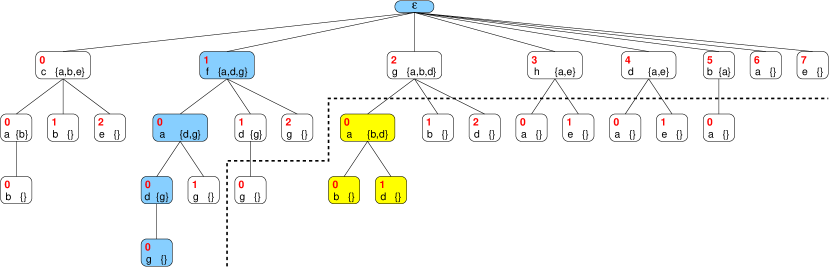
Figure 2: Depiction of an ordered tree. The path in blue identifies the leaf $1000$; the vertices in yellow make up the tree segment rooted at $20$. The vertices below the dashed line are cut off by a sequential branch and bound traversal.

Subtrees and segments

Let $T$ be a tree. A subset $S$ of vertices of $T$ is a subtree of $T$ if $S$ is a tree. Given a vertex $u\in T$, we call the greatest (with respect to set inclusion) subtree $S$ of $T$ with root $u$ the segment of $T$ rooted at $u$. The yellow vertices in Fig. 2 depict the segment $\{{20,200,201}\}$, rooted at vertex $20$.

Two segments of $T$ are overlapping if they intersect non-trivially, in which case one is contained in the other. A set of segments cover the tree $T$ if the prefix-closure of their union equals $T$. That is, if for each $u\in T$ there is a segment $S$ and $v\in S$ such that $u\mathrel{\preceq}v$.

Ordered trees

Trees as defined above capture the parent-child relation (via the prefix order on words) but do not impose any order on siblings. Yet, many tree traversals rely on a specific order on siblings. To be able to express such an order, we generalise the notion of trees to ordered trees. We do so by labeling trees over the natural numbers, using the usual order of the naturals (or rather, its lexicographic extension to words) to order siblings.

Formally, an ordered tree $\lambda$ over $X$ is a function $\lambda:\mathord{\mathit{dom}}(\lambda)\to X^{*}$ such that

• $\mathord{\mathit{dom}}(\lambda)$ is a tree over $\mathbb{N}$,

• the image of $\lambda$ is a tree over $X$, and

• $\lambda$ is an order isomorphism between the two trees, both ordered by the prefix order $\mathrel{\preceq}$.

Since $\lambda$ is an isomorphism of the prefix order the lengths of the words $u$ and $\lambda(u)$ coincide for all $u\in\mathord{\mathit{dom}}(\lambda)$. In an abuse of notation, we write $\lambda$ to denote both the ordered tree (i. e. the function from $\mathord{\mathit{dom}}(\lambda)$ to $X^{*}$) as well as the corresponding tree over $X$ (i. e. the image of the function $\lambda$). When $X$ is understood, we will simply call $\lambda$ an (ordered) tree. To avoid confusion, we will call the elements of $\lambda$ vertices, and the elements of $\mathord{\mathit{dom}}(\lambda)$ positions.

Figure 2 shows an example ordered tree where each node corresponds to the string of red numbers from the root to that node, i.e. a tree over $\mathbb{N}$. The figure also depicts an ordered tree $\lambda$ over the alphabet $X=\{{\textsf{a},\dots,\textsf{h}}\}$, where $\lambda$ maps each position to the string of black letters from the root to the corresponding node. For instance $\lambda$ maps position $1000$ to the string fadg which happens to represent the maximum clique of the graph in Fig. 1.

As $\lambda$ is an order isomorphism the lexicographic ordering on $\mathord{\mathit{dom}}(\lambda)$ carries over to the tree $\lambda$. That is, we define for all $u,v\in\mathord{\mathit{dom}}(\lambda)$, $\lambda(u)\mathrel{\leq_{\mathrm{lex}}}\lambda(v)$ if and only if $u\mathrel{\leq_{\mathrm{lex}}}v$, and $\mathrel{\leq_{\mathrm{lex}}}$ becomes a total ordering on $\lambda$.

We call a function $g:X^{*}\to X^{*}$ an ordered tree generator if all images of $g$ are isograms, i. e. have no repeating letters. Given an ordered tree generator $g$, we define $\lambda_{g}:\mathord{\mathit{dom}}(\lambda_{g})\to X^{*}$ as the function with smallest domain such that

• $\mathord{\mathit{dom}}(\lambda_{g})$ is a tree over $\mathbb{N}$,

• $\lambda_{g}(\epsilon)=\epsilon$, and

• $\lambda_{g}$ is closed under $g$ in the following sense: For all positions $u\in\mathord{\mathit{dom}}(\lambda_{g})$ and corresponding vertices $v=\lambda_{g}(u)$, if $g(v)=a_{0}a_{1}\dots a_{n-1}$ and $i<n$ then $ui$ is a position in $\mathord{\mathit{dom}}(\lambda_{g})$ and $\lambda_{g}(ui)=va_{i}$.

By construction $\lambda_{g}$ is an order isomorphim as images of $g$ are isograms, hence $\lambda_{g}$ is an ordered tree, the ordered tree generated by $g$.

Example: Tree generators for clique problems

Let $G=\langle{V,E}\rangle$ be an undirected graph. Given a vertex $u\in V$, we denote its set of neighbours by $E(u)$.

We define $g:V^{*}\to 2^{V}$ by $g(u_{1}\dots u_{m})=\{{v\in V\mid\forall i:v\neq u_{i}\wedge u_{i}\in E(v)}\}$. Clearly, $g$ is a generator for the tree $t_{g}$ over the alphabet $X=V$, enumerating all cliques of $G$. However, $t_{g}$ enumerates cliques as strings rather than sets and hence every clique of size $k$ will be enumerated $k!$ times.

To avoid enumerating the same clique multiple times, we need to generate an ordered tree where siblings “to the right” avoid vertices that have already been chosen “on the left”. We construct an ordered tree over the alphabet $X=V\times 2^{V}$, where the first component is the latest vertex added to the current clique and the second component is a set of candidate vertices that may extend the current clique. The candidate vertices are incident to all vertices of the current clique, but do not necessarily form a clique themselves. We define the ordered tree generator $h:X^{*}\to X^{*}$ by $h(\langle{u_{1},U_{1}}\rangle\dots\langle{u_{m},U_{m}}\rangle)=\langle{v_{1},V_{1}}\rangle\dots\langle{v_{n},V_{n}}\rangle$ such that

• the $v_{i}$ enumerate the set $U$, and

• the $V_{i}=(U\setminus\{{v_{1},\dots,v_{i-1}}\})\mathbin{\cap}E(v_{i})$

where $U=U_{m}$ if $m>0$, and $U=V$ otherwise. Typically, the $\langle{v_{i},V_{i}}\rangle$ are ordered such that the size of $V_{i}$ decreases as $i$ increases; this order is beneficial for sequential branch and bound traversals.

Clearly, $h$ is an ordered generator for an ordered tree enumerating all cliques of $G$ exactly once (ignoring the second component of the alphabet). Figure 2 shows a tree generated by $h$ for the graph from Fig. 1.

3.2 Maximising Tree Traversals

The trees defined above materialise the search space and order traversals. What is needed for modeling branch-and-bound is an objective function to be computed during traversal and that the search aims to maximise.

Let $Y$ be a set with a total quasi-order $\mathrel{\sqsubseteq}$, that is $\mathrel{\sqsubseteq}$ is a reflexive and transitive, but not necessarily anti-symmetric, total binary relation on $Y$.

Given a tree $T$ over $X$ and an objective function $f:X^{*}\to Y$, the goal is to maximise $f$ over $T$, i. e. to find some $u\in T$ such that $f(u)\mathrel{\sqsupseteq}f(v)$ for all $v\in T$. The objective function is required to be monotonic w. r. t. the prefix order, that is for all $u,u^{\prime}\in X^{*}$, if $u\mathrel{\preceq}u^{\prime}$ then $f(u)\mathrel{\sqsubseteq}f(u^{\prime})$. By monotonicity $f(\epsilon)$ is a minimal element of the image of $f$.

So far, we have modeled maximising tree search. To model branch-and-bound we introduce one additional refinement: A predicate $p$ for pruning subtrees that cannot improve the incumbent. More precisely, the pruning predicate $p:Y\times X^{*}\to\{{0,1}\}$ is a function mapping the incumbent (i. e. the maximal value of $f$ seen so far) and the current vertex to $1$ (for prune) or $0$ (for explore). The pruning predicate must satisfy the following monotonicity and compatibility conditions:

1. For all $y\in Y$ and $u,u^{\prime}\in X^{*}$, if $u\mathrel{\preceq}u^{\prime}$ then $p(y,u)\leq p(y,u^{\prime})$.

2. For all $y,y^{\prime}\in Y$ and $u\in X^{*}$, if $y\mathrel{\sqsubseteq}y^{\prime}$ then $p(y,u)\leq p(y^{\prime},u)$.

3. For all $y\in Y$ and $u\in X^{*}$, if $p(y,u)=1$ then $f(u)\mathrel{\sqsubseteq}y$.

Item 1 implies that all descendents $u^{\prime}$ of a pruned vertex $u$ are also pruned. Item 2 implies a vertex pruned by incumbent $y$ is also pruned by any stronger incumbent $y^{\prime}$. Finally, Item 3 states the correctness of pruning w. r. t. maximising the objective function: Vertex $u$ is pruned by incumbent $y$ only if $f(u)$ does not beat $y$.

How exactly pruning will interact with the tree traversal will be detailed in the next section. Note that pruning is an optimisation and must not be used to constrain the search space. That is, the result of the tree traversal must be independent of the pruning predicate. In particular, the trivial pruning predicate that always returns $0$ (and hence prunes nothing) is a legal predicate.

Example: Objective function and pruning predicate for clique problems

For maximum clique, we set $Y=\mathbb{N}$, and the quasi-order $\mathrel{\sqsubseteq}$ is the natural order $\leq$. We define the objective function $f:X^{*}\to Y$ by $f(w)=|w|$. That is, maximising $f$ means finding cliques of maximum size. We define the pruning predicate $p:Y\times X^{*}\to\{{0,1}\}$ by

$$p(l,\langle{\_,U_{1}}\rangle\dots\langle{\_,U_{m}}\rangle)=\left\{\begin{array}[]{ll}1&\text{if}~{}m>0~{}\text{and}~{}m+|U_{m}|\leq l\\ 0&\text{otherwise}\end{array}\right.$$

That is, pruning decisions rest on the size of the current clique, $m$, and the size of the set of remaining candidate vertices $U_{m}$; vertices will be pruned if adding these two sizes does not exceed the current bound $l$.

3.3 Modelling Multi-threaded Tree Traversals

For this section, we fix an ordered tree $\lambda$ over $X$, which we will traverse according to the order $\mathrel{\leq_{\mathrm{lex}}}$. We also fix an objective function $f:X^{*}\to Y$, and a pruning predicate $p:Y\times X^{*}\to\{{0,1}\}$, where $Y$ is a set with a total quasi-order $\mathrel{\sqsubseteq}$. Finally, we fix a set $\mathit{SEG}$ of pairwise non-overlapping tree segments that cover the tree $\lambda$; we call each segment $S\in\mathit{SEG}$ a task.

State

Let $n\geq 1$ be the number of threads. The state of a backtracking tree traversal is a $(n+2)$-tuple of the form $\sigma=\langle{x,\mathit{Tasks},\theta_{1},\dots,\theta_{n}}\rangle$, where

• $x\in\lambda$ is the incumbent, i. e. the vertex that currently maximises $f$,

• $\mathit{Tasks}\in\mathit{SEG}^{*}$ is a queue of pending tasks, and

• $\theta_{i}$ is the state of the $i$-th thread, where $\theta_{i}=\bot$ if the $i$-th thread is idle, or $\theta_{i}=\langle{S_{i},v_{i}}\rangle$ if $S_{i}\in\mathit{SEG}$ is the $i$-th thread’s current task and $v_{i}\in S_{i}$ the currently explored vertex of that task.

We use Haskell list notation for the task queue $\mathit{Tasks}$. That is, $\mathord{[\,]}$ denotes the empty queue, and $S\mathord{:}\mathit{Tasks}$ denotes a non-empty queue with head $S\in\mathit{SEG}$.

The initial state is $\langle{\epsilon,\mathit{Tasks},\bot,\dots,\bot}\rangle$, where the list $\mathit{Tasks}$ enumerates all tasks in $\mathit{SEG}$, in an arbitrary but fixed order. A final state is of the form $\langle{x,\mathord{[\,]},\bot,\dots,\bot}\rangle$.

Reductions

$$\begin{array}[]{l@{~}l}(\text{strengthen}_{i})\hfil~{}&\displaystyle\frac{f(x)\mathrel{\sqsubset}f(v_{i})}{\langle{x,\mathit{Tasks},\dots,\langle{S_{i},v_{i}}\rangle,\dots}\rangle\to\langle{v_{i},\mathit{Tasks},\dots,\langle{S_{i},v_{i}}\rangle,\dots}\rangle}\\ (\text{schedule}_{i})\hfil~{}&\displaystyle\frac{v_{i}=\text{root of}~{}S\qquad p(f(x),v_{i})=0}{\langle{x,S\mathord{:}\mathit{Tasks},\dots,\bot,\dots}\rangle\to\langle{x,\mathit{Tasks},\dots,\langle{S,v_{i}}\rangle,\dots}\rangle}\\ (\text{prune}_{i})\hfil~{}&\displaystyle\frac{v_{i}=\text{root of}~{}S\qquad p(f(x),v_{i})=1}{\langle{x,S\mathord{:}\mathit{Tasks},\dots,\bot,\dots}\rangle\to\langle{x,\mathit{Tasks},\dots,\bot,\dots}\rangle}\\ (\text{advance}_{i})\hfil~{}&\displaystyle\frac{v_{i}^{\prime}\in S_{i}\qquad v_{i}\mathrel{<_{\mathrm{lex}}}v_{i}^{\prime}\qquad p(f(x),v_{i}^{\prime})=0\qquad\forall v\in S_{i}\,\bigl{(}v_{i}\mathrel{<_{\mathrm{lex}}}v\mathrel{<_{\mathrm{lex}}}v_{i}^{\prime}\Rightarrow p(f(x),v)=1\bigr{)}}{\langle{x,\mathit{Tasks},\dots,\langle{S_{i},v_{i}}\rangle,\dots}\rangle\to\langle{x,\mathit{Tasks},\dots,\langle{S_{i},v_{i}^{\prime}}\rangle,\dots}\rangle}\\ (\text{terminate}_{i})\hfil~{}&\displaystyle\frac{\forall v\in S_{i}\,\bigl{(}v_{i}\mathrel{<_{\mathrm{lex}}}v\Rightarrow p(f(x),v)=1\bigr{)}}{\langle{x,\mathit{Tasks},\dots,\langle{S_{i},v_{i}}\rangle,\dots}\rangle\to\langle{x,\mathit{Tasks},\dots,\bot,\dots}\rangle}\end{array}$$

Figure 3: Reduction rules.

The reduction rules in Fig. 3 define a binary relation $\to$ on states. Each rule carries a subscript indicating which thread it is operating on. Rule $(\text{strengthen}_{i})$ is applicable if the $i$-th thread is not idle and its current vertex $v_{i}$ beats the incumbent on $f$. Of the remaining four rules exactly one will be applicable to the $i$-th thread (unless a final state is reached).

Rules $(\text{schedule}_{i})$ and $(\text{prune}_{i})$ apply if the $i$-th thread is idle and the task queue is non-empty. Which of the two rules applies depends on whether the root vertex $v_{i}$ of the head task $S$ in the queue is to be pruned or not. If not, $S$ becomes the $i$-th thread’s current task and $v_{i}$ the current vertex, otherwise task $S$ is pruned and the $i$-th thread remains idle.

Rules $(\text{advance}_{i})$ and $(\text{terminate}_{i})$ apply if the $i$-th thread is not idle. Which of the two rules applies depends on whether all vertices of the current task $S_{i}$ beyond the current vertex $v_{i}$ (in the lexicographic order $\mathrel{<_{\mathrm{lex}}}$) are to be pruned according to predicate $p$. If so, the $i$-th thread terminates the current task and becomes idle, otherwise the thread advances to the next vertex $v_{i}^{\prime}$ that is not pruned.

It is easy to see that no rule is applicable if and only if all threads are idle and the task queue is empty, that is, iff a final state is reached.

Admissible reductions

The reduction rules in Fig. 3 do not specify an ordering on the rules nor stipulate any restriction on the relative speed of execution of different threads. However, applying the rules in just any order is too liberal. In particular, not selecting rule $(\text{strengthen}_{i})$ when the incumbent could in fact be strengthened may result in missing the maximum. To avoid this, rule $(\text{strengthen}_{i})$ must be prioritised as follows.

We call a reduction $\sigma\to\sigma^{\prime}$ inadmissible if it uses rule $(\text{advance}_{i})$ or $(\text{terminate}_{i})$ even though rule $(\text{strengthen}_{i})$ was applicable in state $\sigma$. A reduction is admissible if it is not inadmissible. Admissible reductions prioritise rule $(\text{strengthen}_{i})$ over rules $(\text{advance}_{i})$ and $(\text{terminate}_{i})$.

By induction on the length of the reduction sequence, one can show that an incumbent $x$ maximises the objective function $f$ over the ordered tree $\lambda$ whenever $\langle{x,\mathord{[\,]},\bot,\dots,\bot}\rangle$ is a final state reachable from the initial state $\langle{\epsilon,\mathit{Tasks},\bot,\dots,\bot}\rangle$ by a sequence of admissible reductions.

We point out that final states are generally not unique. For instance, a graph may contain several different cliques of maximum size, and a parallel maxclique search may non-deterministically return any of these maximum cliques. Therefore the reduction relation cannot be confluent.

Example: Reductions for maxclique

Consider the tree in Fig. 2 encoding the graph in Fig. 1. Let $\mathit{Tasks}=[S_{0},S_{1},S_{2},S_{3},S_{4},S_{5},S_{6},S_{7}]$ be a queue of tasks such that $S_{i}$ is the segment rooted at vertex $i$; for example the segment $S_{2}$ is determined by the set of positions $\{{2,20,200,201,21,22}\}$. Clearly, the $S_{i}$ are pairwise non-overlapping and cover the whole tree. Below, we consider a sample reduction with three threads (with IDs 1 to 3) following a strict round-robin thread scheduling policy, except for selecting the strengthening rule eagerly (that is, as soon as it is applicable). For convenience, we display the reduction rule used in the left-most column and index the reduction arrow with the number of reductions.

$$\begin{array}[]{rcl|l|l}&&\langle{\epsilon,[S_{0},S_{1},S_{2},S_{3},S_{4},S_{5},S_{6},S_{7}],\bot,\bot,\bot}\rangle&\text{pruned}&\text{cut off}\\ (\text{schedule}_{1})&\to_{1}&\langle{\epsilon,[S_{1},S_{2},S_{3},S_{4},S_{5},S_{6},S_{7}],\langle{S_{0},0}\rangle,\bot,\bot}\rangle&&\\ (\text{strengthen}_{1})&\to_{2}&\langle{0,[S_{1},S_{2},S_{3},S_{4},S_{5},S_{6},S_{7}],\langle{S_{0},0}\rangle,\bot,\bot}\rangle&&\\ (\text{schedule}_{2})&\to_{3}&\langle{0,[S_{2},S_{3},S_{4},S_{5},S_{6},S_{7}],\langle{S_{0},0}\rangle,\langle{S_{1},1}\rangle,\bot}\rangle&&\\ (\text{schedule}_{3})&\to_{4}&\langle{0,[S_{3},S_{4},S_{5},S_{6},S_{7}],\langle{S_{0},0}\rangle,\langle{S_{1},1}\rangle,\langle{S_{2},2}\rangle}\rangle&&\\ (\text{advance}_{1})&\to_{5}&\langle{0,[S_{3},S_{4},S_{5},S_{6},S_{7}],\langle{S_{0},00}\rangle,\langle{S_{1},1}\rangle,\langle{S_{2},2}\rangle}\rangle&&\\ (\text{strengthen}_{1})&\to_{6}&\langle{00,[S_{3},S_{4},S_{5},S_{6},S_{7}],\langle{S_{0},00}\rangle,\langle{S_{1},1}\rangle,\langle{S_{2},2}\rangle}\rangle&&\\ (\text{advance}_{2})&\to_{7}&\langle{00,[S_{3},S_{4},S_{5},S_{6},S_{7}],\langle{S_{0},00}\rangle,\langle{S_{1},10}\rangle,\langle{S_{2},2}\rangle}\rangle&&\\ (\text{advance}_{3})&\to_{8}&\langle{00,[S_{3},S_{4},S_{5},S_{6},S_{7}],\langle{S_{0},00}\rangle,\langle{S_{1},10}\rangle,\langle{S_{2},20}\rangle}\rangle&&\\ (\text{advance}_{1})&\to_{9}&\langle{00,[S_{3},S_{4},S_{5},S_{6},S_{7}],\langle{S_{0},000}\rangle,\langle{S_{1},10}\rangle,\langle{S_{2},20}\rangle}\rangle&&\\ (\text{strengthen}_{1})&\to_{10}&\langle{000,[S_{3},S_{4},S_{5},S_{6},S_{7}],\langle{S_{0},000}\rangle,\langle{S_{1},10}\rangle,\langle{S_{2},20}\rangle}\rangle&&\\ (\text{advance}_{2})&\to_{11}&\langle{000,[S_{3},S_{4},S_{5},S_{6},S_{7}],\langle{S_{0},000}\rangle,\langle{S_{1},100}\rangle,\langle{S_{2},20}\rangle}\rangle&&\\ (\text{terminate}_{3})&\to_{12}&\langle{000,[S_{3},S_{4},S_{5},S_{6},S_{7}],\langle{S_{0},000}\rangle,\langle{S_{1},100}\rangle,\bot}\rangle&200,201,21,22&\\ (\text{terminate}_{1})&\to_{13}&\langle{000,[S_{3},S_{4},S_{5},S_{6},S_{7}],\bot,\langle{S_{1},100}\rangle,\bot}\rangle&01,02&\\ (\text{advance}_{2})&\to_{14}&\langle{000,[S_{3},S_{4},S_{5},S_{6},S_{7}],\bot,\langle{S_{1},1000}\rangle,\bot}\rangle&&\\ (\text{strengthen}_{2})&\to_{15}&\langle{1000,[S_{3},S_{4},S_{5},S_{6},S_{7}],\bot,\langle{S_{1},1000}\rangle,\bot}\rangle&&\\ (\text{prune}_{3})&\to_{16}&\langle{1000,[S_{4},S_{5},S_{6},S_{7}],\bot,\langle{S_{1},1000}\rangle,\bot}\rangle&3&30,31\\ (\text{prune}_{1})&\to_{17}&\langle{1000,[S_{5},S_{6},S_{7}],\bot,\langle{S_{1},1000}\rangle,\bot}\rangle&4&40,41\\ (\text{terminate}_{2})&\to_{18}&\langle{1000,[S_{5},S_{6},S_{7}],\bot,\bot,\bot}\rangle&101,11,12&110\\ (\text{prune}_{3})&\to_{19}&\langle{1000,[S_{6},S_{7}],\bot,\bot,\bot}\rangle&5&50\\ (\text{prune}_{1})&\to_{20}&\langle{1000,[S_{7}],\bot,\bot,\bot}\rangle&6&\\ (\text{prune}_{2})&\to_{21}&\langle{1000,[],\bot,\bot,\bot}\rangle&7&\\ \end{array}$$

Figure 4: Example apply reduction rules

We observe that up to reduction 11, the three threads traverse the search tree segments $S_{0}$, $S_{1}$ and $S_{2}$ in parallel. From reduction 12 onwards, the incumbent is strong enough to enable pruning according to the heuristic, i.e. prune if size of current clique plus number of candidates does not beat size of the incumbent. Column pruned lists the positions of the search tree where traversal stopped due to pruning; column cut off list the positions that were never reached due to pruning. The reduction illustrates that parallel traversals potentially do more work than sequential ones in the sense that fewer positions are cut off. Concretely, thread 3 traverses segment $S_{2}$ because the incumbent is too weak; a sequential traversal would have entered $S_{2}$ with the final incumbent and pruned immediately, as indicated by the dashed line in Fig. 2. The reduction also illustrates that parallelism may reduce runtime: a sequential traversal would explore first $S_{0}$ and then $S_{1}$, whereas thread 2 locates the maximum clique in $S_{1}$ without traversing $S_{0}$ first.

4 Generic Branch and Bound Search

This section uses the model in Section 3 as the basis of a Generic Branch and Bound (GBB) API for specifying search problems. The GBB API makes extensive use of higher-order functions, i.e. functions that take functions as arguments, and hence is suitable for parallel implementation in the form of skeletons (Section 5).

We introduce each of the GBB API functions, give their types and show an example of how to use them in a simple implementation of the Maximum Clique problem (Section 2). Later sections show that the API is general enough to encode other branch and bound applications (Sections 6.1 and 6.2).

We start by considering the key types and functions required to specify a general branch and bound search. The API functions and types are specified in Haskell [44] in LABEL:lst:BaBAPI.

⬇

1-- application dependent types

2type Space -- data (e.g. graph) relevant to the problem

3type PartialSolution -- partial solution of the problem

4type Candidates -- set of candidates for extending the partial solution

5type Bound -- "size" of the partial solution; instance of Ord

6

7-- type of nodes making up the search tree

8type Node $=$ (PartialSolution, Candidates, Bound)

9

10-- generates a list of candidate Nodes for extending the search tree by

11-- extending the PartialSolution of the given Node with each of the Candidates

12orderedGenerator :: Space $\rightarrow$ Node $\rightarrow$ [Node]

13

14-- Returns an upper bound on the size of any solution that could result

15-- from extending the given Node’s PartialSolution with any of the given

16-- Candidates

17pruningHeuristic :: Space $\rightarrow$ Node $\rightarrow$ Bound

Listing 1: Generic Branch and Bound (GBB) search API

4.1 Types

The fundamental type for a search is a Node that represents a single position within a search tree (for example in Fig. 2 each box represents a node). This notion of a node differs slightly from the BBM where a single type, $X^{*}$, is used to uniquely identify a particular tree node by the branches leading to it. For an efficient implementation, rather than store an encoding of the branch through the tree, the node type uses the partial solution to encode the branch history and the candidate set to encode potential next steps in the branch. The current bound is maintained for efficiency reasons but could alternatively be calculated from the current solution as in the BBM.

The abstract types are described below, and Table 1 shows how the abstract types map to implementation specific types for Maximum Clique (Section 2), knapsack (Section 6.1) and travelling salesperson (Section 6.2) searches.

Space:

Represents the domain specific structure to be searched.

Solution:

Represents the current (partial) solution at this node. The solution is an application specific representation of a branch within the tree and encodes the history of the search.

Candidates:

Represents the set of candidates that may still be added to the solution to extend the search by a single step. This may be used to encode implementation specific details such as no non-adjacent nodes in a maximum clique search, or simply ensure that no variable is chosen twice.

It is not required that the type of the candidates matches the type the search space. This enables implementation-specific optimisations such as the bitset encoding found in the BBMC algorithm (Section 7.1.1).

Bound:

Represents the bound computed from the current solution. There must be an ordering on bounds, for example as provided by Haskell’s Ord typeclass instance [45] to allow a maximising tree traversal to be performed implicitly using the type.

Node:

Represents a position within the search space. For efficiency it caches the current bound, current solution and candidates for expansion.

Abstract Type	Maximum Clique	Knapsack	TSP
Space	Graph	List of all Items	Distance Matrix
Solution	List of chosen vertices	List of chosen items	Current (partial) Tour
Candidates	Vertices adjacent to all solution vertices	All remaining items	All remaining cities
Bound	Size of the current chosen vertices list	Current profit of items	Current tour length

Table 1: Abstract to concrete type mappings

4.1.1 Function Usage

It is perhaps surprising that the application specific aspects of a branch and bound search can be both precisely specified, and efficiently implemented, with just two functions. The GBB API functions rely on the implicit ordering on the bound type, but could easily be extended to take an ordering function as an argument.

orderedGenerator:

generates the set of candidate child nodes from a node in the space. Search heuristics can be encoded by ordering the child nodes in a list. The search ordering may use these heuristics to provide simple in-order tree traversal or more elaborate heuristics such as depth based discrepancy search (Section 7.1.1).

pruningHeuristic:

returns a speculative best possible bound for the current node. If this bound cannot unseat the global maximum then early backtracking should occur as it is impossible for child nodes to beat the current incumbent.

These functions correspond to the branching and bounding functions respectively. We chose to call them orderedGenerator and pruningHeuristic to highlight their purposes: to generate the next steps in the search and to determine if pruning should occur.

LABEL:lst:maxclique-impl shows instances of these GBB functions that encode a simple, IntSet based, version of the Maximum Clique search. The orderedGenerator builds a set of candidate nodes based on a greedy graph colouring algorithm (colourOrder). The colourings provide a heuristic ordering and, by storing them alongside the solution’s vertices, allow effective bounding to be performed. Candidates only include vertices that are adjacent to every vertex already in the clique. The pruningHeuristic checks if the number of vertices in the current clique and potential colourings can possibly unseat the incumbent. See Section 7.1.1 for instances of the GBB API that use a more realistic bitset encoding [20, 2].

⬇

1type Vertex $=$ Int

2type VertexSet $=$ IntSet

3type Colour $=$ Int

4

5type Space $=$ Graph

6type PartialSolution $=$ ([Vertex], Colour)

7type Candidates $=$ VertexSet

8type Bound $=$ Int

9type Node $=$ (PartialSolution, Bound, Candidates)

10

11colourOrder :: Graph $\rightarrow$ VertexSet $\rightarrow$ [(Vertex, Colour)]

12colourOrder $=$ -- defined elsewhere

13

14-- Reduce a list to a value of type b

15foldl :: (b $\rightarrow$ a $\rightarrow$ b) $\rightarrow$ b $\rightarrow$ [a] $\rightarrow$ b

16foldl f accumulator [] $=$ accumulator

17foldl f accumulator (x:xs) $=$ foldl (f accumulator x) xs

18

19orderedGenerator :: Graph $\rightarrow$ Node $\rightarrow$ [Node]

20orderedGenerator graph ((clique, colour), candidates, size) $=$

21 let choices $=$ colourOrder graph candidates

22 in fst (foldl buildNodes ([], candidates) choices)

23 where

24 buildNodes :: ([Node], VertexSet) $\rightarrow$ (Vertex, Colour) $\rightarrow$ ([Node], VertexSet)

25 buildNnodes (nodes, candidates) (v, colour) $=$ let

26 newClique $=$ (v : clique, colour - 1)

27 newSize $=$ size $+$ 1

28 newCandidates $=$ VertexSet.intersection candidates (adjVertices graph v)

29 -- We delete v from candidates to avoid generating duplicate solutions

30 -- from any vertex "to-the-left" of the current

31 in (nodes $+$$+$ [(newClique, newSize, newCandidates)], VertexSet.delete v candidates)

32

33pruningHeuristic :: Graph $\rightarrow$ Node $\rightarrow$ Bound

34pruningHeuristic g ((clique, colour), bnd, candidates) $=$ bnd $+$ colour

Listing 2: Maximum Clique problem using the GBB API

4.2 General branch and bound Search Algorithm

The essence of a branch and bound search is a recursive function for traversing the nodes of the search space. Algorithm 1 shows the function expressed in terms of the GBB API (LABEL:lst:BaBAPI) where we assume that the incumbent and associated bound are read and written by function calls rather than being explicitly passed as arguments and returned as a result. Hence the final solution is read from the global accessor function instead of the algorithm returning an explicit value. As we are dealing with maximising tree traversals, bounds are always compared using a greater than $(>)$ function defined on the Bound type.

Parallelism may be introduced introduced by searching the set of candidates speculatively in parallel, as illustrated in Section 5. Parallel search branches allow early updates of the incumbent via a synchronised version of the solution read/write interface.

expandSearch (space, node)

begin

       candidates = orderedGenerator(space, node)

       if null(candidates) then

             return

              // Backtrack

            

      // Parallelism may be introduced here

       for c in candidates do

             bestBound = currentBound()

              // built-in function

             localBest = pruningHeuristic(space, node) if localBest $>$ bestBound then

                   if bound(node) $>$ bestBound) then

                         updateBest(solution(node), bound(node))

                          // built-in function

                        

                  expandSearch(space, c)

                  

            return

              // Backtrack

            

      

Algorithm 1 General algorithm for branch and bound search using the GBB API (LABEL:lst:BaBAPI)

4.3 Implementing the GBB API

Although GBB can encode general branch and bound searches, various modifications improve both sequential and parallel efficiency.

Generally the search space is immutable and fixed at the start of the search. In a distributed environment we can avoid copying the search space each time a task is stolen by storing a read only copy of the search space on each host. It is also possible to remove the space argument from the API functions and add accessor functions in the same manner as bound access. The implementations used in Section 7 do pass the space as a parameter.

For some applications, such as Maximum Clique, if the local bound fails to unseat the incumbent then all other candidate nodes to-the-right (assuming an ordered generator) will also fail the pruning predicate. An implementation can take advantage of this fact and break the candidate checking loop for an early backtrack. This optimisation is key in avoiding wasteful search. In the skeleton implementations used in Section 7 we allow this behaviour to be toggled via a runtime flag.

Finally, an implementation can exploit lazy evaluation within the node type to avoid redundant computation. Taking Maximum Clique as an example we can delay the computation of the set of candidates vertices until after the pruning heuristic has been checked (as this only depends on having the bound and colour). Similarly if we use the to-the-right pruning optimisation, described above, we want to avoid paying the cost of generating the nodes which end up being pruned.

5 Parallel Skeletons for Branch and Bound Search

Algorithmic skeletons are higher order functions that abstract over common patterns of coordination and are parameterised with specific computations [3]. For example, a parallel map function will apply a sequential function to every element of a collection in parallel. Skeletons are polymorphic, so the collection may contain elements of any type, and the function type must match the element type. The programmer’s task is greatly simplified as they do not need to specify the coordination behaviour required. The skeleton model has been very influential, appearing in parallel standards such as MPI and OpenMP [46, 47], and distributed skeletons such as Google’s MapReduce [48] are core elements of cloud computing.

Here the focus is on designing skeletons for maximising branch and bound search on distributed memory architectures. These architectures use multiple cooperating processes with distinct memory spaces. The processes may be spread across multiple hosts.

Although it is possible to implement skeletons using a variety of parallelism models, we adopt a task parallel model here. The task parallel model is based around breaking down a problem into multiple units of computation (tasks) that work together to solve a particular problem. In a distributed setting, tasks (and their results) may be shared between processes. For search trees, parallel tasks generally take the form of sub-trees to be searched.

Two skeleton designs are given in this section. The first skeleton, Unordered, makes no guarantees on the search ordering and so may give the anomalous behaviours and the unpredictable parallel performance outlined in  Section 2.2. The second skeleton, Ordered, enforces a strict search ordering and hence avoids search anomalies and gives predictable performance. The unordered skeleton is used as an example of the pitfalls of using a standard random work stealing approach and provides a baseline comparison for evaluating the performance of the Ordered skeleton (Section 7).

We start by considering the key design choices for constructing a branch and bound skeleton. Using these we show how the Unordered skeleton can be constructed, and then show the modifications required to transform the Unordered into the Ordered skeleton. Section 5.4 summarises the design choices and limitations of the design choices are summarised in Section 5.5.

5.1 Design Choices

Three main questions drive the design of branch and bound search skeletons:

1. How is work generated?

2. How is work distributed and scheduled?

3. How are the bounds propagated?

The first two choices focus on task parallel aspects of the design and are common design features for algorithmic skeletons. Bound propagation is a specific issue for branch and bound search and takes the form of a general coordination issue rather than being tied to the task parallel model.

To achieve performance in the task parallel model, tasks should be oversubscribed, that is there should be more tasks than cores, while avoiding low task granularity where communication and synchronisation overheads may outweigh the benefits of the parallel computation. To achieve these characteristics in the skeleton designs a simple approach for work generation is used: generate parallel tasks from the root of the tree until a given depth threshold is reached. This method exploits the heuristic that tasks near the top of the tree are usually of coarse granularity than those nearer the leaves, i.e. they have more of the search space to consider. This threshold approach is commonly used in divide-and-conquer parallelism and allows a large number of tasks to be generated while avoiding low granularity tasks. The argument that tasks near the top of the tree have coarse granularity does not necessarily hold true for all branch and bound searches as variant candidate sets and pruning can truncate some searches initiated near the root of the tree: hence task granularity may be highly irregular.

5.2 Unordered Skeleton

The type signature of the Unordered skeleton is:

⬇

search :: Int -- Depth to spawn to

$\rightarrow$ Node Sol Bnd Candidates -- Root node

$\rightarrow$ (Space $\rightarrow$ Node Sol Bnd Candidates $\rightarrow$ [Node Sol Bnd Candidates]) -- orderedGenerator

$\rightarrow$ (Space $\rightarrow$ Node Sol Bnd Candidates $\rightarrow$ Bool) -- pruningHeuristic

$\rightarrow$ Par Solution

In the skeleton search tasks recursively generate work, i.e. new search tasks. If the depth of a search task does not exceed the threshold it generates new tasks on the host, otherwise the task searches the subtree sequentially.

Work distribution takes the form of random work stealing with exponential back-off [38] and happens at two levels. Intranode steals occur between two workers in the same process, the next sub-tree is stolen from the workqueue of the local process. Only if the worker fails to find local work does an internode steal occur, targeting some random other process. Only one internode steal per process is performed at a time. New tasks, either created by local workers or stolen from remote processes, are added to the local workqueue and are scheduled in last-in-first-out order.

The current incumbent, i.e. best solution, is held on every host, and managed by a distinguished master process. Bound propagation proceeds in two stages. Firstly when a search task discovers a new Solution it sends both the solution and bound to the master and, if no better solution has yet been found, they replace the incumbent. Secondly the master broadcasts the new bound to all other processes, that update their local incumbent unless they have located a better solution. This is a form of eventual consistency [49] on the incumbent. Using this approach, opposed to fully peer to peer, the new solution is sent to the master once and only bounds are broadcast. While broadcast is bandwidth intensive, broadcasting new bounds provides fast knowledge transfer between search tasks. Moreover experience shows that often a good, although not necessarily optimal, bound is found early in the search making bound updates rare. In many applications the bounds are range-limited, e.g. a Maximum Clique cannot be larger than the number of vertices in the graph.

5.3 Ordered Skeleton

The type signature of the Ordered skeleton is as follows.

⬇

search :: Bool -- Diversify search

$\rightarrow$ Int -- Depth to spawn to

$\rightarrow$ Node Sol Bnd Candidates -- Root node

$\rightarrow$ (Space $\rightarrow$ Node Sol Bnd Candidates $\rightarrow$ [Node Sol Bnd Candidates]) -- orderedGenerator

$\rightarrow$ (Space $\rightarrow$ Node Sol Bnd Candidates $\rightarrow$ Bool) -- pruningHeuristic

$\rightarrow$ Par Solution

The additional first parameter enables discrepancy search ordering (Section 7.1.1) to be toggled; an alternative formulation would be to pass an ordering function in explicitly. The skeleton adapts the Unordered skeleton to avoid search anomalies (Section 2.2) and give predictable performance properties as shown in Section 1.

The Sequential Bound property guarantees that parallel runtimes do not exceed the sequential runtime. To maintain this property we enforce that at least one worker executes tasks in the exact same order as the sequential search. The other workers speculatively execute other search tasks and may improve the bound earlier than in the fully sequential case, as illustrated in Fig. 4. Discovering a better incumbent early enables the sequential thread to prune more aggressively and hence explore less of the tree than the entirely sequential search would, providing speedups. While there is no guarantee that the speculative workers will improve the bound, the property will still be maintained by the sequential worker.

Requiring a sequential worker is a departure from the fully random work stealing model. Instead of all workers performing random steals, the task scheduling decisions are enforced for the sequential worker. Our system achieves sequential ordering by duplicating the task information. One set is stealable by any worker, and the other is restricted to the sequential worker. There is a chance that work will be duplicated as some worker may simultaneously attempt to start the same task as the sequential worker. To avoid duplicating work, we use a basic locking mechanism where workers first check whether a task has already started execution before starting the task themselves.

With random scheduling adding a worker may disrupt a good parallel search order (Section 2.2), so to guarantee the non-increasing runtimes property we need to preserve the parallel search order, just as the sequential worker preserves the sequential search order. Preserving the parallel search order means that if with $n$ workers we locate an incumbent by time $t_{pn}$, then with $n+1$ workers we locate the same incumbent, or a better incumbent, at approximately $t_{pn}$. The approximation is required as, in a distributed setting, $t_{pn}$ may vary slightly due to the speed of bound propagation.

It transpires that preserving the parallel search order is also sufficient to guarantee the repeatability property as all parallel executions follow very similar search orders. The parallel search order must be globally visible for it to be preserved, and we can no longer permit random work stealing. Instead all tasks are generated on the master host and maintained in a central priority queue. In our skeleton implementation we use depth-bounded work generate to statically construct a fixed set of tasks, with set priorities, before starting the search. Alternative work generation approaches, for example dynamic generation, are possible provided all tasks are generated on the master host.

The parallel search order may have dramatic effects on search performance [39, 40, 30]. In our skeletons any fixed ordering will maintain the properties, although it may not guarantee good performance. The GBB API in Section 4 relies on the user choosing an ordering of nodes in the orderedGenerator function. This ordering is generally, but not necessarily, based on some domain specific heuristic. One simple scheduling decision, and our default, is to assign priorities from left-most to right-most task in the tree. The skeleton may use any priority order rather than the default left-to-right order, for example the depth-bounded discrepancy (DDS) order [50]. This discrepancy ordering is used when evaluating the Maximum Clique benchmark (Section 7.1.1).

By augmenting the Unordered skeleton with a single worker that follows the sequential ordering and a global priority ordering on tasks we arrive at the Ordered skeleton that provides reliable performance guarantees while still enabling parallelism.

5.4 Skeleton Comparison

Table 2 compares the key design features of the two skeletons. A key difference is where tasks are generated and stored. The Unordered skeleton adopts a dynamic approach at the cost of not giving the same performance guarantees as the Ordered skeleton due to a lack of global ordering. Many other skeleton designs are possible. An advantage of the skeleton approach that exploits a general API is that parallel coordination alternatives may be explored and evaluated without refactoring the application code.

	Unordered	Ordered
Work Generation	Dynamically to depth $d$ on any host	Statically to depth $d$ on master
Work Distribution	Random work stealing all processes	Work stealing master process only
Bounds Propagation	Broadcast	Broadcast
Sequential Worker	False	True

Table 2: Skeleton comparison

5.5 Limitations

For most design choices we have selected a simple alternative. More elaborate alternatives might well deliver better performance. Here we discuss some of the limitations imposed by the simple alternatives selected.

One key limitation of both skeleton designs is the use of depth bounded work generation techniques. While this technique is a well known optimisation for divide and conquer applications, the need to manually tune the depth threshold reduces the skeleton portability as the number of tasks required to populate a system is proportional to the system size. Given the irregular structure of a branch and bound computation it is often difficult to know ahead of time how many tasks will need to be generated to avoid starvation and fully exploit the resources available. In practise we have not found this to be an issue, as for many problem instances such as the three benchmarks used in the skeleton evaluation (Section 6), even generating work to a depth of 1 can give thousands of tasks. However, for some instances, to achieve best performance one may need to split work at much lower levels [30]. An alternative would be to use dynamic work generation techniques where the parallel coordination layer manages load in the system  [51]. Dynamic work generation can cause difficulty for maintaining a global task ordering in a distributed environment such as in the case of the Ordered skeleton.

A consequence of static work generation in the Ordered skeleton is that the runtime for the single worker case can be larger than that of a fully sequential search implementation. With static work generation, work is generated from nodes at a depth $d$ ahead of time and the parent nodes are no longer considered (as they are already searched). This leads to the creation of additional tasks that a sequential implementation may never create due to pruning at the higher levels. The management and searching of these additional tasks causes the discrepancy between the single worker Ordered skeleton and purely sequential search. While this does not effect the properties, as we phrase property 1 in terms of a single worker, it would if a purely sequential implementation in property 1 is considered. The effects of this limitation could be mitigated by treating all nodes above the depth threshold as tasks and allowing cancellation of parent/child tasks. Such an approach complicates the task coordination greatly as tasks require knowledge of both their parent and child task states.

The Ordered skeleton requires additional memory and processing time on the master host to maintain the global task list and respond promptly to work stealing requests. In practise we have not found this to be a significant issue as most tasks near to top of the search tree are long running and the steals occur at irregular intervals. On large distributed systems, and for some searches, it is possible that a single master might prove to be a scalability bottleneck.

5.6 Implementation

The Ordered and Unordered skeletons are implemented in Haskell distributed parallel Haskell (HdpH) embedded Domain Specific Language (DSL) [52]. HdpH has been modified to use a priority queue based scheduler to enable the strict ordering on task execution. While HdpH cannot match the performance of the state of the art branch and bound search implementations it is useful for evaluating the skeletons for the following reasons.

1. HdpH supports the higher order functions, a commonly used approach for constructing skeletons.

2. The HdpH is small and easy to modify, allowing ideas to be rapidly prototyped. For example we experimented with priority-based work stealing.

3. The properties of the Ordered skeleton depend on relative runtime values, i.e. absolute runtime is not the priority.

Although our skeletons have been implemented in a functional language they may be implemented in any system with the following features: task parallelism; work stealing (random/single-source); locking; priority based work-queues/task ordering. Distributed memory skeleton implementations will also require distribution mechanisms and distributed locking.

5.7 Maximum Clique Representation

To end this section we show, using the functions and types defined in LABEL:lst:maxclique-impl how the search skeletons are used within an application. Here we show how the skeleton is called for the Maximum Clique benchmark (Section 2):

⬇

Unordered.search

spawnDepth

(Node ([], 0), 0. allVertices)

orderedGenerator

pruningHeuristic

⬇

Ordered.search

True -- Use discrepancy search

spawnDepth

(Node ([], 0), 0. allVertices)

orderedGenerator

pruningHeuristic

5.8 Other Branch and Bound Skeletons

While algorithmic skeletons are widely used in a range of areas from processing large data sets [48] to multicore programming [53] there has been little work on branch and bound skeletons. Two notable exceptions are MALLBA [54] and Muesli [55] that both provide distributed branch and bound implementations. Both frameworks are written in C++. Muesli uses a similar higher-order function approach to ourselves while MALLBA is designed around using classes and polymorphism to override solver behaviour. In Muesli it is possible to choose between a centralised workpool approach, similar to the Ordered skeleton but using work-pushing rather than work stealing, or a distributed method. Unfortunately the centralised workpool model does not scale well compared with our approach (Section 7). MALLBA similarly uses a single, centralised, workqueue for its branch and bound implementation. The real strength of the MALLBA framework is in the ability to encode multiple exact and inexact combinatorial skeletons as opposed to just branch and bound.

The Muesli authors further highlight the need for reproducible runtimes and note “the parallel algorithm behaves non-deterministically in the way the search-space tree is explored. In order to get reliable results, we have repeated each run 100 times and computed the average runtimes” [55]. By adopting the strictly ordered approach in this paper we avoid the need for large numbers of repeated measurements to account for non-deterministic search ordering.

6 Model, API and Skeleton Generality

To show that the BBM model and GBB API are generic, and to provide additional evidence that the Ordered skeleton preserves the parallel search properties (Section 7) we consider two additional search benchmarks: 0/1 Knapsack, a binary assignment problem, and travelling salesperson, a permutation problem.

6.1 0/1 Knapsack

Knapsack packing is a classic optimisation problem. Given a container of some finite size and a set of items, each with some size and value, which items should be added to the container in order to maximise its value? Knapsack problems have important applications such as bin-packing and industrial decision making processes [56]. There are many variants of the knapsack problem [57], typically changing the constraints on item choice. For example we might allow an item to be chosen multiple times, or fractional parts of items to be selected. We consider the 0/1 knapsack problem where an item may only be selected once and fractional items are not allowed.

At each step a bound may be calculated using a linear relaxation of the problem [58] where, instead of solving for $i\in\{0,1\}$ we instead solve fractional knapsack problem where $i\in[0,1]$. As the greedy fractional approach is optimal and provides an upper bound on the maximum potential value. Although it is possible to compute an upper bound on the entire computation by considering the choices at the top level [59], we do not this here. The primary benefit of this method is to terminate the search early when a maximal solution is found.

A formalisation of the 0/1 Knapsack problem in BBM and the corresponding GBB implementation are given in Appendix B and Appendix C respectively.

6.2 Travelling Salesperson Problem

Travelling salesperson (TSP) is another classic optimisation problem. Given a set of cities to visit and the distance between each city find the shortest tour where each city is visited once and the salesperson returns to the starting city. We consider only symmetric instances where the distance between two cities is the same travelling in both directions.

A formalisation of TSP in BBM and the corresponding GBB implementation are given in Appendix D and Appendix E respectively.

7 Parallel Search Evaluation

This section evaluates the parallel performance of the Ordered and Unordered generic skeletons. It starts by outlining the benchmark instances (Section 7.1) and experimental platform (Section 7.2). We establish a baseline for the overheads of the generic skeletons by comparing them with a state of the art C++ implementation (Section 7.3) of Maximum Clique. Finally we investigate the extent that the Ordered skeleton preserves the runtime and repeatability properties (Section 2.3) for the three benchmarks.

The datasets supporting this evaluation are available from an open access archive [60].

7.1 Benchmark Instances and Configuration

This section specifies how the benchmarks are configured and the instances used. We aim for test instances with a runtime of less than an hour while avoiding short sequential runtimes that don’t benefit from parallelism. These instances ensure we a) have enough parallelism and b) can perform repeated measurements while keeping computation times manageable.

7.1.1 Maximum Clique

The Maximum Clique implementation (Section 2) measured uses the bit set encoded algorithm of San Segundo et al: BBMC [20, 2]. This algorithm makes use of bit-parallel operations to improve performance in the greedy colouring step (orderedGenerator in the GBB API), and ours is the first known distributed parallel implementation of BBMC. We do not use the additional recolouring algorithm [2]. Maximum Clique is one example where prunes can propagate to-the-right (Section 4.3) and we make use of this in the implementation. The instances are given in Table 3 and come from the second DIMACS implementation challenge [61].

brock400_1	brock800_1	MANN_a45	sanr200_0.9
brock400_2	brock800_2	p_hat1000-2	sanr400_0.7
brock400_3	brock800_3	p_hat500-3
brock400_4	brock800_4	p_hat700-3

Table 3: Maximum Clique instances

For many applications, search heuristics are weak and tend to perform badly near the root of the search tree [41]. To overcome this limitation, the Maximum Clique example makes use of a non left-to-right search ordering in order to make the search as diverse as possible. The new order is based on depth-bounded discrepancy search [50] with the algorithm extended to work on n-ary trees by counting the nth child as n discrepancies. An example of the discrepancy search ordering is shown in Fig. 5. This further shows the generality of the skeleton to maintain the properties even when custom search orderings are used.

Figure 5: Discrepancy search priorities - lower is higher priority

7.1.2 The 0/1 Knapsack Problem

The 0/1 Knapsack implementation (Section 6.1) uses ascending profit density ordering as the search heuristic and a greedy fractional knapsack implementation for calculating the lower bound. As with Maximum Clique we take advantage of the prune to-the-right optimisation. The bound is uninitialised at the start the search. This simple implementation does not match the performance of state of the art solvers.

Although the knapsack problem is NP-hard, many knapsack instances are easily solved on modern hardware. Methods exist for generating hard knapsack instances [62]. We make use of the subset of the pre-generated hard instances [63] shown in Table 4.

Instance Name (Pisinger)	Type	Number of Items
knapPI_11_100_1000_37	Uncorrelated span(2,10)	100
knapPI_11_50_1000_40	Uncorrelated span(2,10)	50
knapPI_12_50_1000_23	Weakly Correlated span(2,10)	50
knapPI_12_50_1000_34	Weakly Correlated span(2,10)	50
knapPI_13_50_1000_10	Strongly Correlated span(2,10)	50
knapPI_13_50_1000_32	Strongly Correlated span(2,10)	50
knapPI_14_100_1000_88	Multiple Strongly Correlated	100
knapPI_14_50_1000_64	Multiple Strongly Correlated	50
knapPI_15_500_1000_47	Profit Ceiling	500
knapPI_15_50_1000_20	Profit Ceiling	50
knapPI_16_50_1000_62	Circle	100
knapPI_16_50_1000_21	Circle	50

Table 4: 0/1 Knapsack instances

7.1.3 Travelling Salesperson

The final application is the travelling salesperson problem (Section 6.2). A simple implementation is used that assumes no ordering on the candidate cities and uses Prim’s minimum spanning tree algorithm [64] to construct a lower bound. The initial bound comes from the result of a greedy nearest neighbour search.

Like the knapsack application, this is a proof of concept implementation, based on simple branching and pruning functions, and does not perform as well as current state of the art solvers which go beyond simple branch and bound search.

Problem instances are drawn from two separate locations: the TSPLib instances [65] and random instances from the DIMACS TSP challenge instance generator [66]. A list of benchmarks is given in Table 5.

Name	Type	Cities	Random Seed
burma14	TSPLib	14
ulysses16	TSPLib	16
ulysses22	TSPLib	22
rand_1	DIMACS Challenge	34	22137
rand_2	DIMACS Challenge	35	52156
rand_3	DIMACS Challenge	35	52156
rand_3	DIMACS Challenge	36	62563
rand_4	DIMACS Challenge	37	6160
rand_5	DIMACS Challenge	38	37183
rand_6	DIMACS Challenge	39	50212

Table 5: TSP instances

7.2 Measurement Platform and Protocols

The evaluation is performed on a Beowulf cluster consisting of 17 hosts each with dual 8-core Intel Xeon E5-2640v2 CPUs (2Ghz), 64GB of RAM and running Ubuntu 14.04.3 LTS. Exclusive access to the machines is used and we ensure there is always at least one physical core per thread. Threads are assigned to cores using the default mechanisms of the GHC runtime system.

The skeleton library and applications are written in Haskell using the HdpH distributed-memory parallelism framework as outlined in Section 5.6. Specifically we use the GHC 8.0.2 Haskell compiler and dependencies are pulled from the stackage lts-7.9 repository or fixed commits on github. The complete source code for the experiments is available at: http://dx.doi.org/10.5281/zenodo.254088.

In all experiments, each HdpH node (runtime) is assigned $n$ threads and manages $n-1$ workers that execute the search. The additional thread is used for handling messages from other processes and garbage collection and does not search. The additional thread minimises the performance impact of overheads like communication and garbage collection. Measurements are taken with 1, 2, 4, 8, 32, 64, 128 and 200 workers.

Unless otherwise specified, all results are based on the mean of ten runs. The spawnDepth is always set to one, causing child tasks to be spawned for each top level task. This spawnDepth setting provided good performance for most instances, however it may not be optimal for each individual instance.

7.3 Comparison with a Class-leading C++ Implementation

To establish a performance baseline for the generic Haskell skeletons we compare the sequential (single worker) performance of the skeletons with a state of the art C++ implementation of the Maximum Clique benchmark [30]. Only instances with a (skeleton) sequential runtime of less than one hour are considered.

The C++ results were gathered on a newer system featuring a dual Intel Xeon E5-2697A v4, 512 GBytes of memory, Ubuntu 16.04 and were compiled using g++ 5.4. A single sequential sample is used for comparison.

Table 6 compares the C++ implementation to the Ordered skeleton. To keep the skeleton execution as close to a fully sequential implementation as possible, work is generated only at the top level and is searched in decreasing degree order. As there is no communication, the HdpH node is assigned a single thread and a single worker.

Instance	C++ (s)	Ordered Skeleton (s)	$\frac{\textbf{Ordered Skeleton}}{\textbf{C++}}$
brock400_1	184.4	987.7	5.36
brock400_2	133.7	725.8	5.43
brock400_3	106.1	577.7	5.44
brock400_4	51.6	275.5	5.34
MANN_a45	123.2	238.2	1.93
p_hat1000-2	95.0	421.8	4.44
p_hat500-3	70.9	368.1	5.19
sanr200_0.9	14.3	88.1	6.16
sanr400_0.7	48.3	274.7	5.69

Table 6: Sequential Runtimes of a Class-leading C++ search and the Generic Haskell Ordered Skeleton

As expected, the Ordered skeleton is between a factor of 1.9 and 6.2 slower than the hand crafted C++ search. A primary contributor to the slowdown is Haskell execution time: with the slowdown widely accepted to be a factor of between 2 to 10, but often lower for symbolic computations like these. The slowdown is due to Haskell’s aggressive use of immutable heap structures, garbage collection and lazy evaluation model. The generality of the skeletons means that they use computationally expensive techniques like higher-order functions and polymorphism. Finally, our skeleton implementations have not been extensively hand optimised, as the C++ implementation has.

The remainder of the evaluation uses speedup relative to the one worker Haskell implementation. We argue that the underlying performance in the sequential (one worker) is sufficiently good for the results to be credible.

7.4 Sequential Bound & Non-increasing Runtimes

As Sequential Bound and Non-increasing Runtimes are both runtime properties we evaluate them together. We investigate the relative speedup, or strong scaling, of the Ordered and Unordered skeletons using between 1 and 200 workers for each benchmark. If Sequential Bound holds then the speedup will be greater than or equal to 1, and if Non-increasing Runtimes holds the curves should be non-decreasing. Non-increasing Runtimes is still maintained even when a speedup curve becomes flat: we simply don’t benefit from additional workers.

Figure 6 shows the speedup curves for the Maximum Clique Ordered and Unordered skeletons. Scaling curves are not given for the brock800 series and the p_hat700-3 instances as instances with a one worker baseline of greater than one hour are not considered.

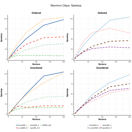
Figure 6: Maximum Clique Speedups: Ordered Skeleton Maintains Sequential Bound and Non-increasing Runtimes Properties

For all Maximum Clique instances both skeletons preserve Sequential Bound, i.e. no configuration has greater runtime than the single worker case. The skeletons achieve good parallel speedups for symbolic computations, delivering a maximum parallel efficiency of around 50%.

The Ordered Skeleton maintains Non-increasing Runtimes for most instances, exceptions being brock400_4, p_hat100-2 and MANN_a45, shown by non-decreasing speedup curves. brock400_4 appears to have the largest slow down between 128 to 200 workers, however the runtime at these scales is tiny (4.5s), and we attribute the slowdown to a combination of (small) parallelism overheads and variability. While the final runtimes for p_hat1000-2 and MANN_a45, once parallelism stops being effective, are larger (15s and 27s respectively) the mean runtimes for 64, 128 and 200 workers are never more than 2.5 seconds apart and this we again attribute to parallelism overheads rather than search ordering issues. Even for instances such as MANN_a45, where there is limited performance benefit for adding additional workers due to a large maximum clique causing increased amounts of pruning, using additional cores never increases runtime significantly.

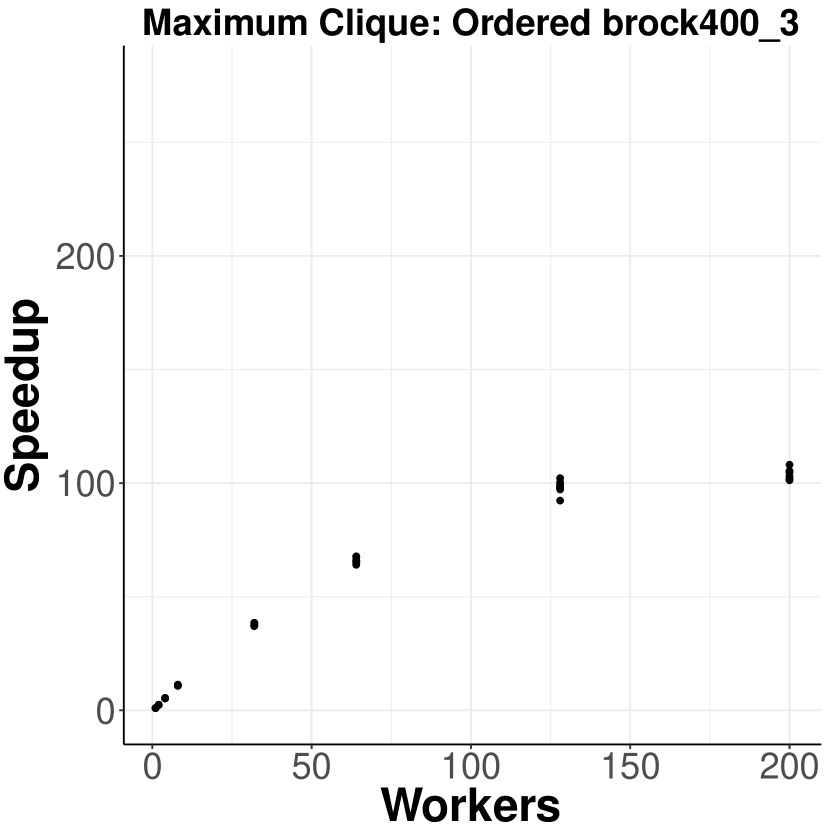
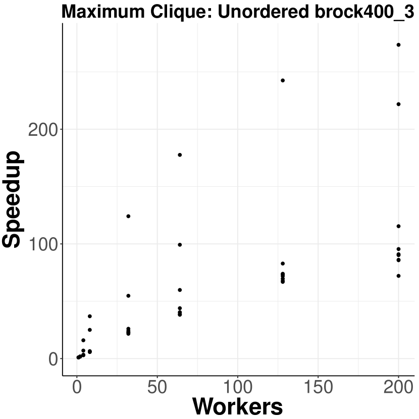
Figure 7: Unordered Skeleton Violates Non-increasing Runtimes: Sampled speedups for Maximum Clique

While the mean speedups reported in Fig. 6 suggest that the Unordered skeleton also preserves Non-increasing Runtimes they disguise the huge runtime variance of the searches. Figure 7 illustrates this by showing each individual speedup sample from the brock400_3 instance. The unpredictable speedups for the Unordered skeleton are in stark contrast to the Ordered skeleton. We attribute the high variance of the Unordered skeleton to the interaction between random scheduling and search ordering.

The speedup curves for the Knapsack and TSP applications are given in Fig. 8 and Fig. 9 respectively. Again any instances with sequential runtimes greater than an hour are excluded.

All travelling salesperson instances, for both skeletons, maintain Sequential Bound. On Knapsack however, in contrast to the Ordered skeleton, the Unordered skeleton deviates from Sequential Bound for five instances: knapPI_11_50_1000_045 (2 – 200 workers), knapPI_11_50_1000_049 (4 – 200 workers), knapPI_14_50_1000_021 (2 – 200 workers), knapPI_15_100_1000_059 (8 – 200 workers) and knapPI_15_50_1000_072 (8 – 200 workers) where the deviation is shown by a speedup of less than one (Fig. 8, bottom).

Non-increasing Runtimes is maintained by the Ordered skeleton in all Knapsack and Travelling Salesperson cases except ulysses16 which shows a slowdown when moving from 32 to 64 workers. As with the brock400_4 slowdown, the runtime at this scale is small (10s), and deviations are likely caused by parallelism overheads rather than search ordering effects.

While it is difficult to directly compare Ordered and Unordered executions due to search ordering effects, in some instances the Unordered skeleton is more efficient than the Ordered skeleton. This is caused by a variety of factors including reduced warm-up time due to not requiring upfront work generation, distributed work stealing reducing the impact of a single node bottleneck and the potential for randomness to find a solution quicker than the fixed search order of the ordered skeleton.

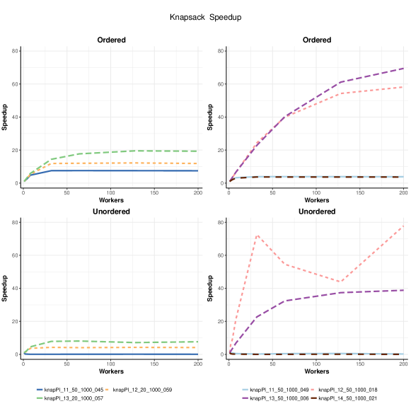
Figure 8: Knapsack Speedups: Ordered Skeleton Maintains Sequential Bound and Non-increasing Runtimes Properties

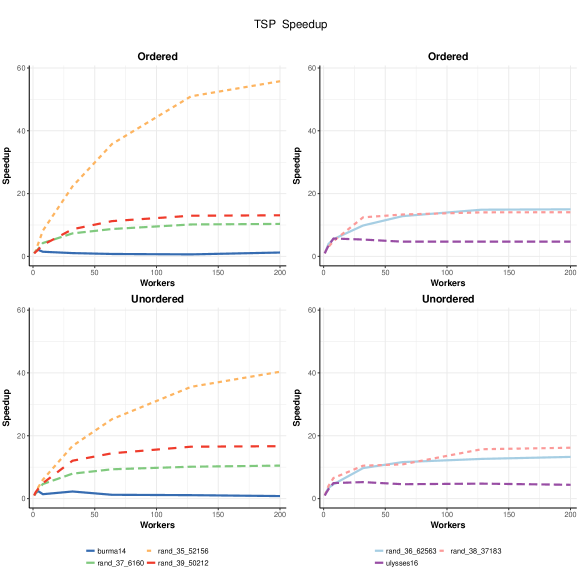
Figure 9: Travelling Salesperson Speedups: Ordered Skeleton Maintains Sequential Bound and Non-increasing Runtimes Properties

7.5 Repeatability

The Repeatability property aims to ensure that multiple runs of the same configuration have similar runtimes. To give a normalised variability measure we use relative standard deviation (RSD), i.e. the ratio of the standard deviation to the mean [67]. To compare the variability of the benchmark instances using the Ordered and Unordered skeletons we plot the RSD as a cumulative distribution function (CDF) for each worker configuration. Here the key metric is how quickly the curve reaches 1, i.e. the point that covers all RSD values. A disadvantage of this type of plot is that it is not robust to outliers. These plots contain all benchmarks including those where the sequential run timed out but a parallel run was successful in less than an hour. Benchmarks with mean runtime less than 5 seconds are removed as a high RSD is expected.

Figure 10 shows the CDF plot for both skeletons for all maximum clique benchmarks run with 1, 8, 64 and 200 workers. With a single worker the maximum RSD of both skeletons is less than 3% showing that they provide repeatable results. This is expected as in the single worker case the Unordered skeleton behaves like the Ordered skeleton, following a fixed left-to-right search order. With multiple workers the Ordered skeleton guarantees better repeatability than the Unordered skeleton, with median RSDs given in Table 7. For the 64 worker case the long tails are caused by outliers in the data and we see a low RSD maintained in almost 90% of cases. The issues with identifying outliers are discussed in Appendix A. The cause of these outliers is unknown but, given the large discrepancy, is probably spurious behaviour on the system rather than a manifestation of search order anomalies.

	Maximum Clique		Knapsack		TSP
Workers	Ordered	Unordered	Ordered	Unordered	Ordered	Unordered
1	2.36	2.29	2.52	2.71	2.40	2.22
2	1.42	4.21	1.24	141.95	1.58	14.52
4	0.94	16.17	1.46	75.51	0.89	9.65
8	0.80	4.60	1.25	107.02	1.84	10.04
32	2.35	10.03	1.94	127.06	4.63	12.77
64	3.52	15.16	1.90	93.12	5.18	13.54
128	3.78	12.19	1.60	110.38	3.08	6.42
200	3.51	15.31	1.99	126.18	3.51	3.89

Table 7: Median Relative Standard Deviation (RSD) % : Ordered Skeleton is more Repeatable

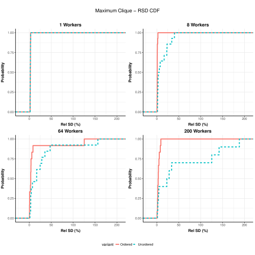
Figure 10: Maximum Clique Relative Variability (CDF of RSD): Ordered Skeleton Maintains Repeatability Property

Figures 11 and 12 show the CDF plots for the knapsack and travelling salesperson benchmarks, and the results are very similar to those for Maximum Clique. With a single worker both Ordered and Unordered skeleton implementations deliver highly repeatable results, i.e. a maximum RSD of less than 3%. The knapsack application has poor repeatability in the Unordered skeleton cases; half of them suffering over 100% RSD. As with Maximum Clique, outlying data points make the Ordered skeleton appear to perform badly on one or two of the TSP benchmarks in the the 64 and 200 worker cases, as discussed in Appendix A. Nonetheless the Ordered skeleton maintains a low RSD.

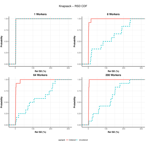
Figure 11: Knapsack Relative Variability (CDF of RSD): Ordered Skeleton Maintains Repeatability Property

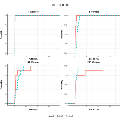
Figure 12: TSP Relative Variability (CDF of RSD): Ordered Skeleton Maintains Repeatability Property. Long Tails are Caused by Data Outliers.

8 Conclusion

Branch and bound searches are an important class of algorithms for solving global optimisation and decision problems. However, they are difficult to parallelise due to their sensitivity to search order, which can cause highly variable and unpredictable parallel performance. We have illustrated these parallel search anomalies and propose that replicable search implementations should avoid them by preserving three key properties: Sequential Bound, Non-increasing Runtimes and Repeatability (Section 2). The paper develops a generic parallel branch and bound skeleton and demonstrates that it meets these properties.

We defined a novel formal model for general parallel branch and bound backtracking search problems (BBM) that is parametric in the search order and models parallel reduction using small-step operational semantics (Section 3). The generality of the model was shown by specifying three benchmarks: Maximum Clique, 0/1 Knapsack and Travelling Salesperson.

We presented a Generic Branch and Bound (GBB) API as a set of higher order functions (Section 4). The GBB API conforms to the BBM and its generality was shown by using it to implement the three benchmarks. The Maximum Clique implementation is the first distributed-memory parallel implementation of San Segundo’s bit parallel Maximum Clique algorithm (BBMC) [2].

We factored the elaborate parallel search behaviours as a pair of sophisticated algorithmic skeletons for distributed memory architectures (Section 5). While the Unordered skeleton does not guarantee the parallel search properties the Ordered skeleton does. For example to guarantee the Sequential Bound one thread is assigned to follow the sequential search order.

We have evaluated the parallel performance of the skeletons with 40 instances of the three benchmark searches (Tables 3, 5 and 4) on a cluster with 17 hosts and up to 200 workers. The sequential performance of the generic skeletons, implemented in Haskell, is between 1.9 and 6.2 times slower than a state of the art Maximum Clique solver implemented in C++. The slowdown is primarily due to the relative execution speeds of Haskell and C++, but also due to the generality of the skeletons and the lack of hand optimisation (Section 7.3).

We evaluated the properties using speedups relative to the sequential runtime of the generic skeletons. We find that the Ordered skeleton preserves the Sequential Bound property for all benchmark instances with non-trivial runtimes. In contrast the Unordered skeleton violates the property for 5 TSP instances (Section 7.4). The Ordered skeleton preserves the Non-increasing Runtimes property for all benchmark instances with non-trivial runtimes. In contrast the Unordered skeleton violates the property for many instances of all three benchmarks (Section 7.4 and Fig. 7). The Ordered skeleton delivers far more repeatable performance than the Unordered skeleton with a median relative standard deviation of 1.78% vs 5.56%, 1.83% vs 87.56% and 1.96% vs 8.61% over all Maximum Clique, Knapsack and TSP instances respectively (Section 7.5).

Acknowledgements

This work is funded by UK EPSRC grants AJITPar (EP/L000687), CoDiMa (EP/M022641), Glasgow DTA (EP/K503058), MaRIONet (EP/P006434), Rathlin (EP/K009931) and Border Patrol (EP/N028201/1). We also thank the anonymous reviewers for their feedback.

References

Appendix A Repeatability and Data Outliers

Unordered	Ordered
120.4	191.8
159.1	192.0
183.0	194.1
183.6	197.1
201.7	197.9
216.6	198.2
220.4	202.7
246.7	206.9
303.4	207.3
619.5	444.0

Table 8: Runtime Outliers in a 32 Worker TSP Instance

Table 8 illustrates some of the issues with outliers in the runtime measurements. The dataset is from the rand_34_22137 TSP instance with 32 workers. The Ordered skeleton runtimes have a potential outlier (in bold) with a runtime 237s greater than any of the other runtimes. The other 9 runtimes have a range of just 15.5s (i.e. 207.3-191.8). In this case it is almost certain that the outlier is not due to some search order effect, but rather to some external system factor, e.g. network contention or some daemon process running. We have not been able to reproduce this effect in additional experiment runs.

The Unordered skeleton runtimes also appear to have an outlier (in bold) with a runtime 316.1s greater than any of the other runtimes. It is, however, harder to be certain that this is an external factor as the variability of the other 9 measurements is far higher, i.e. 183s (303.4-120.4).

As a result of the difficulties of identifying them we have not attempted to eliminate any outliers, even where there is a strong case. That is, the cumulative distribution function (CDF) plots in Figs. 10, 11 and 12 show all measurements recorded. In addition we use median relative standard deviation (RSD) to eliminate the effects of any outliers when comparing the repeatability of the Ordered and Unordered skeletons (Table 7).

Appendix B 0/1 Knapsack – BBM Formalisation

The input parameters for the 0/1 knapsack problem consists of a fixed capacity $C$ and a set of $m$ items $I=\{i_{1}\dots i_{m}\}$. For each item $i_{1}\in I$ we define $p:I\to\mathbb{N}$ and $w:I\to\mathbb{N}$ to be projection functions giving the profit and weight of an item respectively. If the input is considered as a vector of items, then the problem is equivalent to creating an output vector $X$ where $x_{j}\in\{0,1\}$, encoding the inclusion or exclusion of each item $i_{j}$ in the input vector:

$$\textbf{max}\sum_{j=1}^{m}p(i_{j})x_{j}\quad\textbf{where}\;\sum_{j=1}^{m}w(i_{j})x_{j}\leq C$$ (1)

The BBM model uses finite words to represent tree branches. We can trivially extend the profit and weight functions, $p$ and $w$, to those operating on words ($p:I^{*}\to\mathbb{N}$ and $w:I^{*}\to\mathbb{N}$) by taking the sum across each component. An unordered tree generator, $g:I^{*}\to 2^{I}$, takes the current set of items and chooses any item not previously selected:

$$g(i_{1}\dots i_{m})=\{i_{j}\in I\setminus\{i_{1}\dots i_{m}\}~{}|~{}w(i_{1}\dots i_{m})+w(i_{j})\leq C\}$$ (2)

One ordering heuristic is profit density, and an ordered generator simply orders the results of the unordered generator by ascending profit density.

$$\frac{p(i_{1})}{w(i_{1})}\geq\frac{p(i_{2})}{w(i_{2})}\dots\geq\frac{p(i_{n})}{w(i_{n})}$$ (3)

As the aim is to maximise total profit the objective function, $f:I^{*}\to\mathbb{N}$ is simply p, the profit function over words. The ordering on objective functions $\sqsubseteq$ is given by the natural ordering $\leq$.

Finally, the pruning predicate, $p:\mathbb{N}\times I^{*}\to\{0,1\}$, is defined as follows, where fractionalKnapsack greedily solves the residual knapsack problem using continuous relaxation to obtain an optimal solution and hence a bound on the maximal profit.

$$p(bnd,(i_{1}\dots i_{m}))=\begin{cases}1&\textbf{if}\;p(i_{1}\dots i_{m})+fractionalKnapsack(I\setminus\{i_{1}\cdots i_{m}\},C-w(i_{1}\dots i_{m}))\leq bnd\\ 0&otherwise\end{cases}$$ (4)

Appendix C 0/1 Knapsack – GBB and Skeleton Representation

⬇

1type Space $=$ (Array Int Int, Array Int Int)

2type Profit $=$ Int

3type Wight $=$ Int

4type Candidates $=$ [Item]

5data PartialSolution $=$ Solution Capacity [Item] Profit Weight

6

7type KPNode $=$ (PartialSolution, Profit, Candidates)

8

9orderedGenerator :: Space $\rightarrow$ KPNode $\rightarrow$ [KPNode]

10orderedGenerator items (Solution cap is currentProfit currentWeight, bnd, remaining) $=$

11 map createNode (filter (\item $\rightarrow$ currentWeight $+$ (itemWeight items item) $\leq$ cap) remaining)

12 where

13 createNode :: Item $\rightarrow$ KPNode

14 createNode i $=$ let

15 newSol $=$ Solution

16 cap

17 (i:is)

18 (currentProfit $+$ itemProfit items i)

19 (currentWeight $+$ itemWeight items i)

20 newBnd $=$ currentProfit $+$ (itemProfit items i)

21 newCands $=$ delete i remaining

22 in (newSol, newBnd, newCands)

23

24pruningHeuristic :: Space $\rightarrow$ KPNode $\rightarrow$ Int

25pruningHeuristic items (Solution cap (i:is) solP solW, _, _) $=$

26 round $ fractionalKnapsack items solP solW (i $+$ 1)

27

28-- Defined elsewhere. Solve knapsack allowing for fractional values

29fractionalKnapsack :: Space $\rightarrow$ Profit $\rightarrow$ Weight $\rightarrow$ Int $\rightarrow$ Double

30

31-- Calling a skeleton implementation

32Unordered.search

33 spawnDepth

34 (KPNode (Solution cap items 0 0, 0, items))

35 orderedGenerator

36 pruningHeuristic

Listing 3: Knapsack in the GBB API

A Knapsack implementation using the GBB API and the Unordered skeleton is shown in LABEL:lst:GBBKnapsack. The implementation comes directly from BBM, generating only candidate items which do not exceed the capacity constraint and using continuous relaxation to compute an upper bound. The Unordered.search function on line 32 invokes the Unordered skeleton implementation with an empty root node. The Ordered skeleton invocation is very similar. A higher performance version supporting distributed execution is used for evaluating the skeletons in Section 7.1.2.

Appendix D Travelling Salesperson – BBM Formalisation

The TSP input consists of a set $C$ of $n$ cities and a metric on $C$, given by a symmetric non-negative distance function $d:C\times C\to\mathbb{R}$.

Tours are modelled as words over $C$ where the word $t=c_{1}c_{2}\dots c_{k}\in C^{*}$ represents a (partial) tour starting at $c_{1}$ and ending at $c_{k}$ if all cities $c_{i}$ are pairwise distinct. The tour $t$ is complete if $k=n$, that is, if every city in $C$ is visited exactly once.

We generalize the distance function $d$ to words in $C^{*}$ in the obvious way:

$$d(\epsilon) =0$$

$$d(c_{1}) =0$$

$$d(c_{1}\dots c_{k}c_{k+1}) =d(c_{1}\dots c_{k})+d(c_{k},c_{k+1})$$

The (unordered) tree generator function, $g:C^{*}\to 2^{C}$, extends a partial tour with each city that hasn’t been visited yet, enumerating all possible tours. Due to symmetries — rotations to change the start, reflections to change the direction — each tour is enumerated $2n$ times. This symmetry can be broken by fixing the starting city.

$$g(c_{1}\dots c_{k}) =C\setminus\{c_{1},\dots,c_{k}\}$$

The objective function, $f:C^{*}\to\mathbb{R}$, maps complete tours to the total distance travelled (including the distance from the last city back to the starting city) and incomplete tours to infinity :

$$f(c_{1}\dots c_{k}) =\begin{cases}d(c_{1}\dots c_{k}c_{1})&\text{if $c_{1}\dots c_{k}$ is a complete tour}\\ \infty&\text{otherwise}\end{cases}$$

We aim to minimise the objective function with respect to the standard order $\leq$ on the reals; in BBM this corresponds to maximising $f$ with regard to the dual order $\geq$ on $\mathbb{R}$ where $\infty$ is the minimal element w. r. t. $\geq$.

Finally, the pruning predicate, $p:\mathbb{R}\times C^{*}\to\{0,1\}$, prunes a partial tour if the distance travelled along the tour plus the weight of a minimum spanning tree covering the remaining cities exceeds the distance of the current shortest tour:

$$p(\mathit{minDist},c_{1}\dots c_{k})=\begin{cases}1&\text{if}~{}d(c_{1}\dots c_{k})+\mathit{weightMST}(C\setminus\{c_{2},\dots,c_{k-1}\})\geq\mathit{minDist}\\ 0&\text{otherwise}\end{cases}$$

Here, $\mathit{weightMST}(C\setminus\{c_{2},\dots,c_{k-1}\})$ is the weight of a minimum spanning tree covering the not-yet visited cities as well as the starting city $c_{1}$ and the most recently visited city $c_{k}$. The weight of this MST is a lower bound of the distance covered in the shortest partial tour from $c_{k}$ through the not-yet visited cities in $C\setminus\{c_{1},\dots,c_{k}\}$ and back to the start $c_{1}$.

Appendix E Travelling Salesperson – GBB and Skeleton Representation

⬇

1type City $=$ Int

2type Path $=$ [City]

3type Candidates $=$ IntSet

4type Solution $=$ (Path, Int)

5type TSPNode $=$ (Solution, Int, Candidates)

6

7orderedGenerator :: DistanceMatrix $\rightarrow$ TSPNode $\rightarrow$ [TSPNode]

8orderedGenerator distances ((path, pathLen), bnd, remainngCities) $=$

9 map constructNode remainngCities

10 where

11 constructNode :: City $\rightarrow$ TSPNode

12 constructNode city $=$

13 let newPath $=$ path $+$$+$ city

14 newDist $=$ pathLen $+$ distanceBetween (last path) city

15 newRemainngCities $=$ delete city remainngCities

16 in

17 if not (null newRemainngCities) then

18 ((newPath, newDist), bnd, newRemainngCities)

19 else

20 -- Only update the bound when we have a complete path

21 let newPath’ $=$ newPath $+$$+$ first path

22 newDist’ $=$ newDist $+$ distanceBetween (last newPath) (first path)

23 in ((newPath’, newDist’), newDist’, [])

24

25pruningHeuristic :: DistanceMatrix $\rightarrow$ TSPNode $\rightarrow$ Int

26pruningHeuristic dists ((path, pathLen), bnd, remainngCities) $=$

27 pathLen $+$ weightMST dists (last path) (insert (first path) remainngCities)

28

29-- Defined elsewhere. Compute the minimum spanning tree cost via Prim’s algorithm

30weightMST :: DistanceMatrix $\rightarrow$ City $\rightarrow$ [City] $\rightarrow$ Int

31

32-- Calling a skeleton implementation

33Unordered.search

34 spawnDepth

35 (TSPNode (([1],0), greedyNearestNeighbour cities, delete 1 cities))

36 orderedGenerator

37 pruningHeuristic

Listing 4: TSP in the GBB API

A TSP implementation using the GBB API and Unordered skeleton is shown in LABEL:lst:GBBTSP. Unlike in the Maximum Clique and Knapsack benchmarks, bound updates only happen when there are no cities left to choose which requires additional logic in the orderedGenerator function. When calling the skeleton on line 33, the root node sets an initial solution with the initial city selected single city selected. The bounds are initially set to the result of a greedy nearest neighbour algorithm to improve early pruning.

References

-
[1]
G. Laporte,
The
vehicle routing problem: An overview of exact and approximate algorithms,
European Journal of Operational Research 59 (3) (1992) 345 – 358.
doi:http://dx.doi.org/10.1016/0377-2217(92)90192-C.
URL http://www.sciencedirect.com/science/article/pii/037722179290192C - [2] P. San Segundo, F. Matia, D. Rodriguez-Losada, M. Hernando, An improved bit parallel exact maximum clique algorithm, Optimization Letters 7 (3) (2011) 467–479.
- [3] M. Cole, Algorithmic Skeletons: Structured Management of Parallel Computation, MIT Press, Cambridge, MA, USA, 1991.
-
[4]
J. D. Eblen, C. A. Phillips, G. L. Rogers, M. A. Langston,
The maximum clique
enumeration problem: Algorithms, applications and implementations, in:
J. Chen, J. Wang, A. Zelikovsky (Eds.), Bioinformatics Research and
Applications, Vol. 6674 of Lecture Notes in Computer Science, Springer Berlin
Heidelberg, Berlin, Heidelberg, 2011, pp. 306–319.
doi:10.1007/978-3-642-21260-4_30.
URL http://dx.doi.org/10.1007/978-3-642-21260-4_30 - [5] S. Butenko, W. E. Wilhelm, Clique-detection models in computational biochemistry and genomics, European Journal of Operational Research 173 (1) (2006) 1–17. doi:10.1016/j.ejor.2005.05.026.
-
[6]
J. Konc, D. Janežič,
A branch and bound
algorithm for matching protein structures, in: B. Beliczynski,
A. Dzielinski, M. Iwanowski, B. Ribeiro (Eds.), Adaptive and Natural
Computing Algorithms, Vol. 4432 of Lecture Notes in Computer Science,
Springer Berlin Heidelberg, 2007, pp. 399–406.
doi:10.1007/978-3-540-71629-7_45.
URL http://dx.doi.org/10.1007/978-3-540-71629-7_45 -
[7]
D. Fukagawa, T. Tamura, A. Takasu, E. Tomita, T. Akutsu,
A clique-based method
for the edit distance between unordered trees and its application to analysis
of glycan structures, BMC Bioinformatics 12 (Suppl 1) (2011) S13.
doi:10.1186/1471-2105-12-S1-S13.
URL http://www.biomedcentral.com/1471-2105/12/S1/S13 -
[8]
M. Depolli, J. Konc, K. Rozman, R. Trobec, D. Janežič,
Exact parallel maximum
clique algorithm for general and protein graphs, Journal of Chemical
Information and Modeling 53 (9) (2013) 2217–2228.
arXiv:http://pubs.acs.org/doi/pdf/10.1021/ci4002525, doi:10.1021/ci4002525.
URL http://pubs.acs.org/doi/abs/10.1021/ci4002525 - [9] B. Yan, S. Gregory, Detecting communities in networks by merging cliques, in: Intelligent Computing and Intelligent Systems, 2009. ICIS 2009. IEEE International Conference on, Vol. 1, 2009, pp. 832–836. doi:10.1109/ICICISYS.2009.5358036.
-
[10]
Y. Okubo, M. Haraguchi, Finding
conceptual document clusters with improved top-n formal concept search, in:
Proceedings of the 2006 IEEE/WIC/ACM International Conference on Web
Intelligence, WI ’06, IEEE Computer Society, Washington, DC, USA, 2006, pp.
347–351.
doi:10.1109/WI.2006.81.
URL http://dx.doi.org/10.1109/WI.2006.81 -
[11]
I. M. Bomze, M. Budinich, P. M. Pardalos, M. Pelillo,
The
maximum clique problem, Handbook of Combinatorial Optimization (Supplement
Volume A) 4 (1999) 1–74.
URL http://citeseerx.ist.psu.edu/viewdoc/summary?doi=10.1.1.56.6221 -
[12]
P. San Segundo, D. Rodríguez-Losada, F. Matía, R. Galán,
Fast exact feature based
data correspondence search with an efficient bit-parallel MCP solver,
Applied Intelligence 32 (3) (2010) 311–329.
doi:10.1007/s10489-008-0147-6.
URL http://dx.doi.org/10.1007/s10489-008-0147-6 -
[13]
C. McCreesh, S. N. Ndiaye, P. Prosser, C. Solnon,
Clique and constraint
models for maximum common (connected) subgraph problems, in: Principles and
Practice of Constraint Programming - 22nd International Conference, CP
2016, Toulouse, France, September 5-9, 2016, Proceedings, 2016, pp. 350–368.
doi:10.1007/978-3-319-44953-1_23.
URL http://dx.doi.org/10.1007/978-3-319-44953-1_23 - [14] G. Regula, B. Lantos, Formation control of quadrotor helicopters with guaranteed collision avoidance via safe path, Electrical Engineering and Computer Science 56 (4) (2013) 113–124.
- [15] D. J. Johnson, M. A. Trick (Eds.), Cliques, Coloring, and Satisfiability: Second DIMACS Implementation Challenge, Workshop, October 11-13, 1993, American Mathematical Society, Boston, MA, USA, 1996.
-
[16]
P. Prosser, Exact algorithms for
maximum clique: A computational study, Algorithms 5 (4) (2012) 545–587.
doi:10.3390/a5040545.
URL http://dx.doi.org/10.3390/a5040545 -
[17]
E. Tomita, T. Seki, An
efficient branch-and-bound algorithm for finding a maximum clique, in:
Discrete Mathematics and Theoretical Computer Science, 4th International
Conference, DMTCS 2003, Dijon, France, July 7-12, 2003. Proceedings, 2003,
pp. 278–289.
doi:10.1007/3-540-45066-1_22.
URL http://dx.doi.org/10.1007/3-540-45066-1_22 -
[18]
E. Tomita, T. Kameda, An
efficient branch-and-bound algorithm for finding a maximum clique with
computational experiments, J. Global Optimization 37 (1) (2007) 95–111.
doi:10.1007/s10898-006-9039-7.
URL http://dx.doi.org/10.1007/s10898-006-9039-7 -
[19]
E. Tomita, Y. Sutani, T. Higashi, S. Takahashi, M. Wakatsuki,
A simple and faster
branch-and-bound algorithm for finding a maximum clique, in: WALCOM:
Algorithms and Computation, 4th International Workshop, WALCOM 2010, Dhaka,
Bangladesh, February 10-12, 2010. Proceedings, 2010, pp. 191–203.
doi:10.1007/978-3-642-11440-3_18.
URL http://dx.doi.org/10.1007/978-3-642-11440-3_18 -
[20]
P. S. Segundo, D. Rodríguez-Losada, A. Jiménez,
An
exact bit-parallel algorithm for the maximum clique problem, Computers &
Operations Research 38 (2) (2011) 571 – 581.
doi:http://dx.doi.org/10.1016/j.cor.2010.07.019.
URL http://www.sciencedirect.com/science/article/pii/S0305054810001504 -
[21]
C. McCreesh, P. Prosser,
Reducing the branching
in a branch and bound algorithm for the maximum clique problem, in:
Principles and Practice of Constraint Programming - 20th International
Conference, CP 2014, Lyon, France, September 8-12, 2014. Proceedings, 2014,
pp. 549–563.
doi:10.1007/978-3-319-10428-7_40.
URL http://dx.doi.org/10.1007/978-3-319-10428-7_40 -
[22]
A. Nikolaev, M. Batsyn, P. S. Segundo,
Reusing the same
coloring in the child nodes of the search tree for the maximum clique
problem, in: Learning and Intelligent Optimization - 9th International
Conference, LION 9, Lille, France, January 12-15, 2015. Revised Selected
Papers, 2015, pp. 275–280.
doi:10.1007/978-3-319-19084-6_27.
URL http://dx.doi.org/10.1007/978-3-319-19084-6_27 -
[23]
P. S. Segundo, C. Tapia,
Relaxed approximate
coloring in exact maximum clique search, Computers & OR 44 (2014)
185–192.
doi:10.1016/j.cor.2013.10.018.
URL http://dx.doi.org/10.1016/j.cor.2013.10.018 -
[24]
C. Li, Z. Fang, K. Xu,
Combining MaxSAT reasoning
and incremental upper bound for the maximum clique problem, in: 2013 IEEE
25th International Conference on Tools with Artificial Intelligence, Herndon,
VA, USA, November 4-6, 2013, 2013, pp. 939–946.
doi:10.1109/ICTAI.2013.143.
URL http://dx.doi.org/10.1109/ICTAI.2013.143 -
[25]
C. Li, H. Jiang, R. Xu,
Incremental MaxSAT
reasoning to reduce branches in a branch-and-bound algorithm for
MaxClique, in: Learning and Intelligent Optimization - 9th International
Conference, LION 9, Lille, France, January 12-15, 2015. Revised Selected
Papers, 2015, pp. 268–274.
doi:10.1007/978-3-319-19084-6_26.
URL http://dx.doi.org/10.1007/978-3-319-19084-6_26 -
[26]
P. S. Segundo, A. Nikolaev, M. Batsyn,
Infra-chromatic bound for
exact maximum clique search, Computers & OR 64 (2015) 293–303.
doi:10.1016/j.cor.2015.06.009.
URL http://dx.doi.org/10.1016/j.cor.2015.06.009 -
[27]
Q. Wu, J. Hao, A review on
algorithms for maximum clique problems, European Journal of Operational
Research 242 (3) (2015) 693–709.
doi:10.1016/j.ejor.2014.09.064.
URL http://dx.doi.org/10.1016/j.ejor.2014.09.064 -
[28]
C. McCreesh, P. Prosser,
Multi-threading a state-of-the-art
maximum clique algorithm, Algorithms 6 (4) (2013) 618–635.
doi:10.3390/a6040618.
URL http://dx.doi.org/10.3390/a6040618 -
[29]
M. Depolli, J. Konc, K. Rozman, R. Trobec, D. Janezic,
Exact parallel maximum clique
algorithm for general and protein graphs, Journal of Chemical Information
and Modeling 53 (9) (2013) 2217–2228.
doi:10.1021/ci4002525.
URL http://dx.doi.org/10.1021/ci4002525 -
[30]
C. McCreesh, P. Prosser, The shape of
the search tree for the maximum clique problem and the implications for
parallel branch and bound, ACM Trans. Parallel Comput. 2 (1) (2015)
8:1–8:27.
doi:10.1145/2742359.
URL http://doi.acm.org/10.1145/2742359 -
[31]
J. Xiang, C. Guo, A. Aboulnaga,
Scalable maximum clique
computation using mapreduce, in: C. S. Jensen, C. M. Jermaine, X. Zhou
(Eds.), 29th IEEE International Conference on Data Engineering, ICDE
2013, Brisbane, Australia, April 8-12, 2013, IEEE Computer Society, 2013,
pp. 74–85.
doi:10.1109/ICDE.2013.6544815.
URL http://dx.doi.org/10.1109/ICDE.2013.6544815 -
[32]
D. R. Morrison, S. H. Jacobson, J. J. Sauppe, E. C. Sewell,