Universal Extra Dimensions and the Graviton Portal to Dark Matter

Abstract

The Universal Extra Dimension (UED) paradigm is particularly attractive as it not only includes a natural candidate for the Dark Matter particle , but also addresses several issues related to particle physics. Non-observations at the Large Hadron Collider, though, has brought the paradigm into severe tension. However, a particular 5-dimensional UED model emerges from a six dimensional space-time with nested warping. The $AdS_{6}$ bulk protects both the Higgs mass as well as the UED scale without invoking unnatural parameter values. The graviton excitations in the sixth direction open up new (co-)annihilation channels for the Dark Matter particle, thereby allowing for phenomenological consistency, otherwise denied to the minimal UED scenario. The model leads to unique signatures in both satellite-based experiments as well as the LHC.
Keywords: Dark Matter, UED, Graviton, Warped Compactification

1 Introduction

The presence of dark matter (DM) in the universe and its dominance over luminous matter is well-established [1, 2]. What is not apparent, though, is its nature, a consequence of the lack of any evidence (direct or indirect) barring the astrophysical/cosmological context. Furthermore, the absence of any DM candidate within the Standard Model (SM) requires us to propose scenarios going beyond. The primary requirement is to have at least one component that is stable over cosmological times scales. Very often, this stability is guaranteed by a $Z_{2}$ symmetry, with the DM (and, possibly, its heavier cousins) being odd under it and all SM particles being even.

It would be particularly appealing if any such theory can also address at least some of the several other outstanding issues in the SM. Most notable of the latter are the hierarchy problem, the mechanism of generating the baryon asymmetry in the universe, the flavor problem (including the large hierarchy in the fermion masses), the unification of forces, etc.. Two particular classes that address most (if not all) of these issues are provided by supersymmetry and/or extra-dimensional scenarios. Here, we concentrate on the latter alternative.

The RS-model [3, 4, 5] provided a particularly elegant resolution of the hierarchy, between the quantum-gravity scale $M_{5}$ and the electroweak scale $v$. through $v=\tilde{v}\,\exp(-\pi\,k_{5}\,r_{c})$, where $\tilde{v}={\cal O}(M_{5})$ and $k_{5}$ denotes the bulk curvature, and $r_{c}$ is the stabilized value of the modulus. Some of the aforementioned issues (as also proton decay and FCNC) can be addressed too if the SM gauge fields and fermions are not restricted to the TeV brane (as in the original RS model), but are promoted to 5-dimensional ones. Constraints from the electroweak precision tests as well as other low-energy observables necessitates the introduction of additional symmetries and fields, though. Existence of a viable DM-candidate requires even further additions. More damaging, though, is the non-observation of any Kaluza-Klein (KK) excitation of the graviton at the LHC, namely the constraint $m_{1}\mathrel{\hbox to0.0pt{\raise 2.15277pt\hbox{$>$}\hss}{\lower 2.15277pt\hbox{$\sim$}}}4\,{\rm TeV}$ (at 95%C.L.)  [6, 7] On the other hand, the model implies $m_{n}=x_{n}\,k_{5}\,\exp(-\pi\,k_{5}\,r_{c})$, where $x_{n}$ are the roots of the Bessel function of order one. With the applicability of semi-classical arguments [8] (upon which the model hinges) as well as arguments relating the D3 brane tension to the string scale (and, hence, to $M_{5}$ through Yang-Mills gauge couplings) restricting $k_{5}/M_{5}\mathrel{\hbox to0.0pt{\raise 2.15277pt\hbox{$<$}\hss}{\lower 2.15277pt\hbox{$\sim$}}}0.15$, one would, thus, expect the first KK-mode to be, at best, a few times heavier than the Higgs, and the non-observation implies at least a little hierarchy.

The Universal Extra Dimension (UED) scenario [9, 10], on the other hand, envisages a flat compactified fifth dimension of radius $R$ and a $S^{1}/Z_{2}$ orbifolding (thereby ensuring that zero mode fermions are chiral in nature) with all the SM fields allowed to propagate in the bulk. Although KK-number is broken, in the absence of any brane-localized terms in the Lagrangian, a $Z_{2}$-subgroup (“KK-parity”) is retained. Given by $(-1)^{n}$ where $n$ is the KK-level, this renders the lightest KK-excitation absolutely stable. With the mass of the $n^{\rm th}$ mode of a species (with a five-dimensional mass $m_{0}$) being given by

$$m_{n}^{2}=m_{0}^{2}+n^{2}/R^{2}\ ,$$ (1.1)

clearly the excitations of a given level are nearly degenerate for $R^{-1}\mathrel{\hbox to0.0pt{\raise 2.15277pt\hbox{$>$}\hss}{\lower 2.15277pt\hbox{$\sim$}}}1\,{\rm TeV}$. However, quantum corrections (due to both the bulk fields as well as the orbifolding) provide additional splitting, resulting in $B^{(1)}$ (the first excitation of the hypercharge boson) being the lightest, and, hence, the DM candidate [11, 12, 13, 14]. With all interactions being determined by the SM gauge action, the pair production of the KK-excitations at colliders is unsuppressed (barring kinematics), leading to the possibility of striking signatures. The non-observation of such states at the LHC, whether it be monojet searches at $\sqrt{s}=8\,{\rm TeV}$ [15, 16] or multijets at $\sqrt{s}=8\,{\rm TeV}$ [17, 18], has been used to impose constraints of $R^{-1}\mathrel{\hbox to0.0pt{\raise 2.15277pt\hbox{$>$}\hss}{\lower 2.15277pt\hbox{$\sim$}}}1150\,{\rm GeV}$ [19]. Subsequent simulations [20, 21] suggest that the bound can be strengthened to $R^{-1}\mathrel{\hbox to0.0pt{\raise 2.15277pt\hbox{$>$}\hss}{\lower 2.15277pt\hbox{$\sim$}}}1400\,{\rm GeV}$. On the other hand, agreement with the observed DM energy density [1, 2] suggests that $R^{-1}\mathrel{\hbox to0.0pt{\raise 2.15277pt\hbox{$<$}\hss}{\lower 2.15277pt\hbox{$\sim$}}}1400\,{\rm GeV}$ [22], an upper bound that cannot be relaxed as the interactions are well-specified and the mass-differences constrained. A further refinement of the search strategies, including a count of (soft) particle multiplicities [23] would impose even stronger constraints. Thus, we are approaching an era of tension and the model stands to be comprehensively ruled out. A further, and unrelated, problem with the UED paradigm is that there is no mechanism to stabilize the modulus $R$, thereby leaving it free to change with time, assuming any value.

2 Model

To solve both these problems in a unified manner, we consider a six-dimensional space-time with successive (nested) warpings along the two compactified dimensions, which are individually $Z_{2}$-orbifolded with 4-branes sitting at each of the edges. The uncompactified directions ($x^{\mu})$ support four-dimensional Lorentz symmetry. With the compact directions represented by the angular coordinates $x_{4,5}\in[0,\pi]$ and the corresponding moduli by $R_{y}$ and $r_{z}$, the line element is, thus, given by [24]

$$ds^{2}_{6}=b^{2}(x_{5})[a^{2}(x_{4})\eta_{\mu\nu}dx^{\mu}dx^{\nu}+R_{y}^{2}dx_{4}^{2}]+r_{z}^{2}dx_{5}^{2}\ ,$$ (2.1)

where $\eta_{\mu\nu}$ is the flat metric on the four-dimensional slice of spacetime.

Denoting the fundamental scale in six dimensions by $M_{6}$ and the negative (six dimensional) bulk cosmological constant by $\Lambda_{6}$, the total bulk-brane action is, thus,

$$\begin{array}[]{rcl}{\cal{S}}&=&\displaystyle{\cal{S}}_{6}+{\cal{S}}_{5}\\[6.45831pt] {\cal{S}}_{6}&=&\displaystyle\int d^{4}x\,dx_{4}\,dx_{5}\sqrt{-g_{6}}\,(M_{6}^{4}R_{6}-\Lambda_{6})\\[6.45831pt] {\cal{S}}_{5}&=&\displaystyle\int d^{4}x\,dx_{4}\,dx_{5}\sqrt{-g_{5}}\,[V_{1}(x_{5})\,\delta(x_{4})+V_{2}(x_{5})\,\delta(x_{4}-\pi)]\\ &+&\displaystyle\int d^{4}x\,dx_{4}\,dx_{5}\sqrt{-\tilde{g}_{5}}\,[V_{3}(x_{4})\,\delta(x_{5})+V_{4}(x_{4})\,\delta(x_{5}-\pi)]\ .\end{array}$$ (2.2)

The five-dimensional metrics in ${\cal S}_{5}$ are those induced on the appropriate 4-branes which accord a rectangular box shape to the space.

The action above, augmented by the choice of the line element as in eqn.(2.1) leads to straightforward Einstein equations. However, before listing them, it should be pointed out that the solutions as presented in the original paper, viz. Ref.[24], were not the most general ones. Rather, they had assumed specific values for the induced five-dimensional cosmological constants on the 4-branes (and, similarly, for the four-dimensional cosmological constants on the 3-branes). Relaxing this allows for more generic solutions, including the existence of bent branes. For example, if an induced four-dimensional cosmological constant $\Omega$ were to be admitted, the four dimensional components of the Einstein equations would read [25, 24]

$$a^{2}\left[\frac{3}{R_{y}^{2}}\left(\frac{a^{\prime\prime}}{a}+\frac{a^{\prime 2}}{a^{2}}\right)+\frac{2}{r_{z}^{2}}\left(3\dot{b}^{2}+2b\ddot{b}+\frac{\Lambda_{6}\,r_{z}^{2}}{2M_{6}^{4}}b^{2}\right)\right]=\frac{\Omega}{r_{z}^{2}}\ ,$$

where primes(dots) denote derivatives with respect to $x_{4}$ ($x_{5}$). The aforementioned induced cosmological constant (on a five dimensional hypersurface along constant ($x_{5}$) makes an appearance in the form of a constant of separation $\widetilde{\Omega}$, leading to

$$3\dot{b}^{2}+2b\ddot{b}+\frac{\Lambda_{6}\,r_{z}^{2}}{2M_{6}^{4}}b^{2}=\widetilde{\Omega}$$ (2.3)

and

$$\frac{3}{R_{y}^{2}}\left(\frac{a^{\prime\prime}}{a}+\frac{a^{\prime 2}}{a^{2}}\right)+\frac{2}{r_{z}^{2}}\widetilde{\Omega}=\frac{\Omega}{r_{z}^{2}\,a^{2}}\,.$$ (2.4)

Only if the induced five-dimensional cosmological constant $\widetilde{\Omega}$ vanishes identically, does the nonlinear differential equation for $b(x_{5})$ simplify to yield a special class of solutions [25] that are untenable for $\widetilde{\Omega}\neq 0$. However, rather than limit ourselves to this fine-tuned case, we consider the generic case. It is interesting to note, though, that the two solutions are very similar differing, at most, by 50% (almost independent of the value of $\widetilde{\Omega}$) [25]. Assuming $\widetilde{\Omega}<0$, the first equation has the solution

$$\begin{array}[]{rclcl}b(x_{5})&=&\displaystyle b_{1}\cosh(k|x_{5}|+b_{2})\\[8.61108pt] b_{1}&=&\displaystyle\sqrt{\frac{-\widetilde{\Omega}}{3\,k^{2}}}&=&\displaystyle{\rm sech}(k\pi+b_{2})\\[8.61108pt] k&=&\displaystyle r_{z}\sqrt{\frac{-\Lambda_{6}}{10\,M_{6}^{4}}}&\equiv&\displaystyle r_{z}\,M_{6}\,\epsilon\ ,\end{array}$$ (2.5)

where the second equality in the second line is nothing but the normalization $b(x_{5}=\pi)=1$. The dimensionless constant $\epsilon$ is a measure of the bulk cosmological constant $\Lambda_{6}$ in terms of the fundamental scale $M_{6}$. Clearly, if $\epsilon$ is too large, the bulk would be highly warped and a semiclassical treatment (as is being attempted here) would be invalid. Typically, it has been argued that $\epsilon\mathrel{\hbox to0.0pt{\raise 2.15277pt\hbox{$<$}\hss}{\lower 2.15277pt\hbox{$\sim$}}}0.15$, by arguments relating the brane tension to the scale of some underlying string theory (or even to $M_{6}$) [8]. Although somewhat larger values can be admitted, this would entail the applicability of the semiclassical approximation growing progressively worse. On the other hand, the aforementioned limit automatically ensures that the curvature in the $x_{4}$-direction is sufficiently small.

The generic solution to eqn.(2.4) for a nonzero $\Omega$, is also given in terms of hyperbolic functions and is quite complicated. The subsequent algebra is rendered extremely complex and does not offer easy insights. On the other hand, the observed cosmological constant in our world is infinitesimally small and we must live close to $\Omega=0$. Hence, we shall assume that $\Omega=0$. While this may be termed a fine-tuning, it is, at worst, exactly the same as that in the RS model. Indeed, $\Omega=0$ is not a special solution, and a similar criticism could be made against any finite value for $\Omega$. On the other hand, $\Omega=0$ could, in principle, have resulted from some as yet unspecified symmetry [26]. In this limit, the solution can be expressed as

$$a(x_{4})=e^{-c|x_{4}|}\ ,\qquad c\equiv b_{1}\,k\,\frac{R_{y}}{r_{z}}\ ,$$ (2.6)

where we have normalized by imposing $a(x_{4}=0)=1$. The graviton has a tower of towers. The modes in the $x_{4}$-direction are given in terms of Bessel functions, while those in the $x_{5}$-direction are given in terms of associated Legendre functions [27]. This change, along with the fact of the hierarchy resolution now being shared between two warpings, results in the mass of the first KK-mode being significantly higher than that of the corresponding mode in the RS case. Furthermore, the large coupling enhancement that allowed for the RS-gravitons to be extensively produced at the LHC, is now tempered to a significant degree [27]. Consequently, the production rates are suppressed and the scenario easily survives the current bounds [27, 28].

The brane potentials are determined by the junction conditions. The ones at $x_{5}=0,\pi$ are simple and are given by

$$V_{3}=\frac{-8M_{6}^{4}k}{r_{z}}\tanh(b_{2})\ ,\qquad V_{4}=\frac{8M_{6}^{4}k}{r_{z}}\tanh(k\pi+b_{2})\ ,$$ (2.7)

whereas the ones at $x_{4}=0,\pi$ have $x_{5}$–dependent tensions

$$V_{1}(x_{5})=-V_{2}(x_{5})=\frac{8M_{6}^{4}c}{R_{y}\,b(x_{5})}=\frac{8M_{6}^{4}k}{r_{z}}\,{\rm sech}(k|x_{5}|+b_{2})\ .$$ (2.8)

It should be noted that the Israel junction condition $V_{1}=-V_{2}$ is the consequence of choosing $\Omega=0$, or, in other words, a configuration wherein the four-dimensional cosmological constant vanishes exactly. Had we chosen to work with $\Omega\neq 0$, this equality of magnitude would not have held. This is exactly analogous to the case of the vanilla RS model.

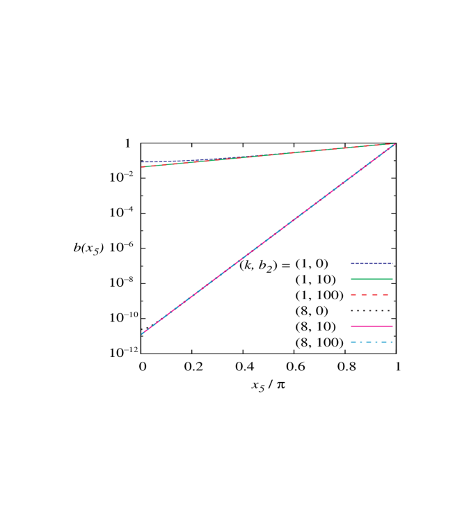
Figure 1: The warp function $b(x_{5})$ for some choices of the parameters.

In Fig.1, we show the metric element $b(x_{5})$ for several choices of the parameters $k$ and $b_{2}$. It is quite apparent that, for a given $k$, the warp factor depends very little on $b_{2}$. While some difference is still noticeable for small $k$ values, for slightly larger $k$, the almost marginal difference is concentrated close to $x_{5}=0$.

Given this relative insensitivity, it is conceivable that limiting values of $b_{2}$ may be used to understand the main features and the results for intermediate values of $b_{2}$ may be obtained by interpolating between such extreme cases. Some of these limits lead to significant algebraic simplifications, opening the possibility of closed-form analytic solutions. For example, choosing $b_{2}=0$ recovers the results of Ref.[24] and we have

$$\begin{array}[]{rcl}c&=&\displaystyle\frac{R_{y}\,k}{r_{z}}\,{\rm sech}(k\pi)\\[8.61108pt] V_{1}(x_{5})&=&\displaystyle-V_{2}(x_{5})=\frac{8M_{6}^{4}k}{r_{z}}{\rm sech}(k|x_{5}|)\,,\\[8.61108pt] V_{3}&=&0\\[4.30554pt] V_{4}&=&\displaystyle\frac{8M_{6}^{4}k}{r_{z}}\,\tanh(k\pi)\,\,.\end{array}$$ (2.9)

This corresponds to a bent brane scenario with non-vanishing induced five-dimensional cosmological constants on the hypersurfaces at $x_{5}=0,\pi$. This could easily be seen by observing that the induced metric on the $x_{5}=0$ surface, apart from an overall $b(0)$ factor, is given by

$$ds_{5}^{2}=e^{-2c|x_{4}|}\eta_{\mu\nu}dx^{\mu}dx^{\nu}+R_{y}^{2}dx_{4}^{2}\,\,,$$

or, in other words, the induced geometry is $AdS_{5}$-like.

3 Naturally Stabilised UED

We are particularly interested in the limit opposite to that discussed at the end of the preceding section, namely, in a sufficiently large $b_{2}$. For such values, $b(x_{5})\approx(b_{1}/2)\exp(k|x_{5}|+b_{2})$. For sufficiently large $b_{2}$, we have $c\ll k$ (see eqn.2.6), no matter how large the ratio $R_{y}/r_{z}$ might be. With $c\rightarrow 0$ the brane potentials now read

$$\begin{array}[]{rcl}V_{1}=-V_{2}&\approx&0\\[4.30554pt] V_{3}&\approx&\displaystyle\frac{-8M_{6}^{4}k}{r_{z}}\approx-V_{4}\ .\end{array}$$ (3.1)

The fact of $V_{3}\approx-V_{4}$ reveals the near vanishing of the cosmological constant induced on the brane. As for the line element, in this limit,

$$ds^{2}=e^{2k(|x_{5}|-\pi)}\Big{(}e^{-2c|x_{4}|}\eta_{\mu\nu}dx^{\mu}dx^{\nu}+R_{y}^{2}dx_{4}^{2}\Big{)}+r_{z}^{2}dx_{5}^{2}$$

$$\approx e^{2k(|x_{5}|-\pi)}\Big{(}\eta_{\mu\nu}dx^{\mu}dx^{\nu}+R_{y}^{2}dx_{4}^{2}\Big{)}+r_{z}^{2}dx_{5}^{2}\ .$$

This metric is conformally flat and along with the $AdS_{6}$ bulk, it resembles a generalization of the Randall-Sundrum geometry in 5-dimensions. With this simplification, the 4-brane tensions are rendered pairwise equal and opposite [25], reflecting the vanishing of the induced cosmological constant on the branes.

It should be realized, though, that the approximate conformal flatness would have followed as long as $c\ll k$. We do not strictly need either of $b_{2}\to\infty$ or $c\to 0$. A sufficiently large $b_{2}\mathrel{\hbox to0.0pt{\raise 2.15277pt\hbox{$>$}\hss}{\lower 2.15277pt\hbox{$\sim$}}}75$ would lead to $c\mathrel{\hbox to0.0pt{\raise 2.15277pt\hbox{$<$}\hss}{\lower 2.15277pt\hbox{$\sim$}}}10^{-22}$ (a value that will be shown to be small enough to support a viable DM candidate) and qualitatively the same conclusions as a larger $b_{2}$.

Choosing a particular value for $b_{2}$ (this choice also served to determine $c$) that corresponds to a small $\widetilde{\Omega}$ represents a small five-dimensional cosmological constant (equivalently, straight, or unbent, four-branes at the ends of the world). The opposite limit corresponds to the case wherein the four-branes suffer the maximum possible bending commensurate with a semiclassical analysis (or, in other words, a five-dimensional cosmological constant comparable to the fundamental scale). The low energy phenomenology, naturally, would turn out to be quite different in the two cases. Clearly, any intermediate value of $b_{2}$ would correspond to a intermediate value of the five-dimensional cosmological constant and, similarly, for the low-energy phenomenology.

We now turn to the issue of stabilization. Contrary to the RS case, here we need to stabilize two moduli, namely $r_{z}$ and $R_{y}$. The former can be trivially stabilized a la Goldberger-Wise [29] through the introduction of a bulk scalar with a simple quadratic potential, which, when integrated out, provided the requisite effective potential for the radion [25]. Of course, such a scalar field contributes to the energy density of the bulk and the solution for the metric would be altered. However, with the space-time now close to being conformally flat, $r_{z}$ can be stabilized (including backreaction) through a introduction of a bulk scalar with a quartic potential [25], and a closed-form solution for both the scalar and the graviton wavefunction obtained. The resultant distortion of the graviton spectrum and the couplings thereof is minimal. With the natural scale on the 4-brane at $x_{5}=\pi$ now being warped down to the TeV-scale, a scalar localized on this brane would be expected to stabilize $R_{y}^{-1}$ to the same scale. Indeed, as Ref.[25] points out, an analogous exercise can also be undertaken towards stabilizing $R_{y}$ with a scalar now introduced on the brane at $x_{5}=0$. While this is technically correct, it should be noted that, for values of $c$ that we require from the DM perspective, the corresponding potential needs to be a very shallow one, thereby calling into question the stability. However, this issue can be viewed from a different perspective. The very fact that the warping in the $x_{5}$-direction stipulates an energy scale, of ${\cal O}(10\,{\rm TeV})$ on the brane at $x_{5}=0$ implies that any dynamics on this brane must be at energies lower than this scale. On the other hand, in the absence of any other restraining mechanism, masses would tend to rise to the maximum possible scale. In other words, one would expect $R_{y}^{-1}$ to lie somewhat below the fundamental energy scale on this brane.

It is also interesting to consider the effect of a rolling $R_{y}$. This can be done by promoting $R_{y}$ to a dynamical field (in the same spirit as a radion is stabilized) and examine its evolution as a function of time. While first indications are that this is a slow process, we shall desist from a full discussion at this point.

Considering the SM fields to be five-dimensional ones, defined on the entire 4-brane at $x_{5}=0$, leads, now, to a stabilized 5-dimensional UED-like scenario. With the Higgs field being localized on the TeV brane (the 4-brane located at $x_{5}=0$), we have

$$m_{\rm Higgs}=\gamma\,r_{z}^{-1}\,e^{-k\pi}\ ,$$ (3.2)

a relation bearing close resemblance to the 5D one. Here, $\gamma/r_{z}$ is the Higgs mass at the UV brane, ($r_{z}^{-1}$ being the natural scale) with $\gamma$ encompassing both the possible small hierarchy between the fundamental parameters as well as quantum corrections to the measurable. In delineating parameter space, we use $1>\gamma\mathrel{\hbox to0.0pt{\raise 2.15277pt\hbox{$>$}\hss}{\lower 2.15277pt\hbox{$\sim$}}}0.7$. Note, here, that the lower limit is not sacrosanct, but has been motivated by the aesthetic desire of not introducing a large “little hierarchy”.

Before we end this section, let us take a look at a concrete measure of the sensitivity of the Higgs mass to the key parameter, namely $b_{2}$. The analogue of the well-known Barbieri-Guidice naturalness parameter [30, 31] is given by

$$\zeta=\frac{\partial\ln(m_{\rm Higgs}(b_{2})/m_{0})}{\partial\ln(b_{2})}\qquad m_{0}\equiv\gamma\,r_{z}^{-1}\ .$$ (3.3)

Using the relations derived in this section, we present, in Fig. 2, this parameter as a function of $b_{2}$ for a relevant choice of $(k,\epsilon)$ and three choices of the product $M_{6}\,R_{y}$. It can be seen easily that $\zeta$ is acceptably small for $b_{2}$ values of interest ($\mathrel{\hbox to0.0pt{\raise 2.15277pt\hbox{$>$}\hss}{\lower 2.15277pt\hbox{$\sim$}}}70$). Even though $\zeta$ can become large for larger values of the product $M_{6}\,R_{y}$, the fine-tuning becomes unacceptably large only for $b_{2}\sim 15$, far away from the range of interest.

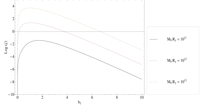
Figure 2: The Barbieri-Giudice parameter $\zeta$ as a function of $b_{2}$ for $k=8$, $\epsilon=0.15$ and three different values of the product $M_{6}\,R_{y}$.

4 Gravitons and their Interactions

The (four-dimensional) Planck mass, in such theories is a derived quantity rather than a fundamental one and is obtained by integrating the action over $x_{4,5}$, thereby yielding

$$M_{\rm Pl}^{2}=(M_{6}^{3}R_{y}\pi/3\epsilon)\,\left[1-\exp(-3k\pi)\right]\ .$$ (4.1)

With $\epsilon\mathrel{\hbox to0.0pt{\raise 2.15277pt\hbox{$<$}\hss}{\lower 2.15277pt\hbox{$\sim$}}}0.15$ and $R_{y}^{-1}\ll M_{6}$, we clearly have $M_{6}\ll M_{\rm Pl}$. This is markedly different from the case of the original RS model and has considerable phenomenological consequences [27, 32]. Expanding the graviton wavefunction as

$$h_{\mu\nu}(x_{\mu},x_{4},x_{5})=\frac{1}{\sqrt{R_{y}r_{z}}}\sum_{n,p}h^{(n,p)}_{\mu\nu}(x_{\mu})\Psi_{n}(x_{4})\chi_{p}(x_{5})\ ,$$ (4.2)

the equation of motion for the $x_{5}$ component is

$$\left[\partial_{5}(b^{5}\partial_{5})+m_{p}^{2}b^{3}\right]\chi_{p}(x_{5})=0\ ,$$

with the solution being given in terms of associated Legendre functions [27]. For large $b_{2}$ though, these simplify [32], in terms of $\tilde{z}\equiv e^{k(\pi-x_{5})}$

$$\chi_{p}\approx\displaystyle N_{p}^{-1}\,\tilde{z}^{5/2}\left[J_{5/2}\left(m_{p}\,r_{z}\,k^{-1}\tilde{z}\right)+\beta_{p}Y_{5/2}\left(m_{p}\,r_{z}\,k^{-1}\tilde{z}\right)\right]\,$$ (4.3)

where the constants $N_{p}$ are determined from the normalization conditions

$$\int_{-\pi}^{\pi}dx_{5}\,b^{3}\chi_{p}\chi_{p^{\prime}}=\delta_{p,p^{\prime}}\ .$$ (4.4)

The Neumann boundary conditions ($\chi^{\prime}_{p}$ vanishing at both $x_{5}=0,\pi$) demand that $\beta_{p}$ be vanishingly small and

$$m_{p}=k\,e^{-k\pi}\,r_{z}^{-1}\,x_{p}$$

where $x_{p}$ are the roots of $J_{3/2}(x)$. As for the equation of motion for $\Psi_{n}(x_{4})$, in this regime of small $c$, it is almost a flat Laplacian, and we have, for the masses of the 4-dimensional graviton modes $h^{(n,p)}_{\mu\nu}(x_{\mu})$,

$$m_{np}^{2}=p_{4}^{2}+p_{5}^{2}\approx n^{2}\,R_{y}^{-2}+m_{p}^{2}\ .$$

and

$$\Psi_{n}(x_{4})=\frac{1}{2\pi}+\frac{\cos(nx_{4})}{\pi}\ .$$ (4.5)

With the $x_{4}$-direction being nearly flat, $(-1)^{n}$ is a very good symmetry for gravitons and the SM-fields alike. With the latter being expressible in terms of $\sin(n\,x_{4})$ and $\cos(n\,x_{4})$, we have, for the graviton interactions,

$$\begin{array}[]{rcl}{\cal L}_{\rm int.}&=&\displaystyle\int_{0}^{\pi}\frac{dx_{4}}{M_{6}^{2}}\,h_{\mu\nu}(x_{\mu},x_{4},x_{5}=0)T^{\mu\nu}(x_{\mu},x_{4})\end{array}$$ (4.6)

where the energy momentum tensor $T^{\mu\nu}(x_{\mu},x_{4})$ for gauge field(G) and fermion field(F) is expressible as

$$\begin{array}[]{rclcl}T_{G}^{\mu\nu}(x_{\mu},x_{4})&=&\displaystyle\frac{1}{2\pi R_{y}}T_{G}^{(0,0)}(x_{\mu})&+&\displaystyle\sum_{n^{\prime},m=1}\frac{1}{\pi R_{y}}T_{G}^{(n^{\prime},m)}(x_{\mu})\cos(n^{\prime}x_{4})\cos(mx_{4})\\[12.91663pt] T_{F}^{\mu\nu}(x_{\mu},x_{4})&=&\displaystyle\frac{1}{2\pi R_{y}}T_{Fl}^{(0,0)}(x_{\mu})&+&\displaystyle\sum_{n^{\prime},m=1}\frac{1}{\pi R_{y}}T_{Fl}^{(n^{\prime},m)}(x_{\mu})\cos(n^{\prime}x_{4})\cos(mx_{4})\\[4.30554pt] &&&+&\displaystyle\sum_{n^{\prime},m=1}\frac{1}{\pi R_{y}}T_{Fr}^{(n^{\prime},m)}(x_{\mu})\sin(n^{\prime}x_{4})\sin(mx_{4})\ ,\end{array}$$ (4.7)

the difference between the left ($l$) and right ($r$) fermion modes accruing from the different boundary conditions [32]. Using eqns.(4.7 & 4.5) and integrating the $x_{4}$ and $x_{5}$ directions, we get

$$\begin{array}[]{rcl}{\cal L}_{\rm int.}&=&\displaystyle\sum_{p,n^{\prime}=0}C^{(0,p)}_{n^{\prime}}h^{(0,p)}_{\mu\nu}(x_{\mu})\,T^{\mu\nu(n^{\prime},n^{\prime})}_{i}(x_{\mu})+\sum_{n,p,n^{\prime}=1}C^{(n,p)}_{n^{\prime}}h^{(n,p)}_{\mu\nu}(x_{\mu})\,T^{\mu\nu(n^{\prime},|n\pm n^{\prime}|)}_{i}(x_{\mu})\\[10.76385pt] &=&\displaystyle\sum_{n,p,n^{\prime}=0}^{\infty}C^{(n,p)}_{n^{\prime}}h^{(n,p)}_{\mu\nu}(x_{\mu})\,T^{\mu\nu(n^{\prime},|n\pm n^{\prime}|)}_{i}(x_{\mu})\end{array}$$ (4.8)

where $i\in G,F$. For our analysis, the only relevant graviton is the first excitation in the $x_{5}$ direction namely $h^{(0,1)}_{\mu\nu}$. And the only relevant ones if its couplings are those to the SM fields (namely, $C^{(0,1)}_{0}$) and their first KK-modes in the $x_{4}$ direction (viz. $C^{(0,1)}_{1}$). These are actually identical, and we use the compact notation

$$\begin{array}[]{rcl}C^{0,1}\equiv C^{(0,1)}_{0}=C^{(0,1)}_{1}=\displaystyle\frac{1}{4\pi}\;\frac{\chi_{1}(x_{5}=0)}{M_{6}^{2}\sqrt{R_{y}r_{z}}}\ .\end{array}$$ (4.9)

Using eqns.(4.3 & 4.4), the common coupling $C^{0,1}$ can be expressed in terms of the parameters of the theory in a straightforward way. What is important to note is that $C^{0,1}$ cannot vary immensely as long as the extent of the warping is not changed drastically. This is quite similar to the case of the RS scenario where, for the first KK-graviton, the (dimensionful) coupling to the SM fields is only somewhat smaller than $m_{\rm graviton}^{-1}$. Much the same happens here. There is a small further suppression [27] owing to two factors. For one, the extent of the hierarchy (between the fundamental scale and the IR scale) is somewhat different owing to the presence of an extra direction. Moreover the graviton wavefunction at $x_{5}=0$ is somewhat modified from the RS case (in the case at hand, this transpires in the orders of the Bessel functions).

5 The Relic Density

Within the mUED, the $B^{(1)}$ turns out to be the lightest of the KK-excitations, and owing to the existence of a KK-parity (namely, the $Z_{2}$ symmetry of $x_{4}\leftrightarrow-x_{4}$) is exactly stable. In the present case, the truth of $B^{(1)}$ being the lightest still continues to hold. However, the non-vanishing of $c$ explicitly breaks the KK-parity, and would induce decays of the $B^{(1)}$. The leading role in such decays is played by a tree-level KK parity-violating vertex connecting the $B^{(1)}$ to a pair of SM fermions, generated on KK-reduction in the presence of the slightly warped background. In the small $c$ limit, the corresponding vertex factor is given by

$$\mathcal{V}\approx-i~{}g_{1}\,Y_{f}~{}\gamma_{\mu}~{}\frac{\sin(\pi+c~{}\pi^{2}/2)}{\pi}\approx i\,\frac{g_{1}\,c\,\pi}{2}\,Y_{f}\,\gamma_{\mu}$$

where $g_{1}$ is the $U(1)_{Y}$ coupling and $Y_{f}$ the hypercharge of the fermion. The total (fermionic) decay width is, thus, given by

$$\Gamma_{B^{(1)}\rightarrow{\rm fermions}}\approx\frac{\pi\,g_{1}^{2}\,c^{2}}{48}\;M_{B^{(1)}}\;\sum_{f}Y_{f}^{2}\,C_{f}\,\left(1-4\frac{m_{f}^{2}}{M_{B_{1}}^{2}}\right)\,\left(1+2\frac{m_{f}^{2}}{M_{B_{1}}^{2}}\right)$$

where $C_{f}$ is the number of colors and the sum extends over all fermions. Decays into scalars(operative in the radion higgs mixing) are of no importance.Thus, for the DM to be stable over cosmological timescales, one needs $c\mathrel{\hbox to0.0pt{\raise 2.15277pt\hbox{$<$}\hss}{\lower 2.15277pt\hbox{$\sim$}}}10^{-22}$. Note that such values of $c$ are engendered by $b_{2}\mathrel{\hbox to0.0pt{\raise 2.15277pt\hbox{$>$}\hss}{\lower 2.15277pt\hbox{$\sim$}}}75$, a region that is commensurate with desirably low values of the Barbieri-Giudice sensitivity measure (see. Fig.2).

Owing to their near degeneracy in mass and similarity of couplings, the generic first KK-excitation does not decouple much earlier than the $B^{(1)}$. Consequently, they play an important role in determining the relic density $n_{B^{(1)}}$, not only through co-annihilations, but also by replenishing $B^{(1)}$ through processes like $e^{(1)+}e^{-}\to B^{(1)}+\gamma$. Indeed, for mUED, the latter effect is strong enough that the inclusion of these excitations, especially the singlets, forces down $R^{-1}$ by nearly 250 GeV [22, 33]. The exact magnitudes of such effect depends on the quantum corrections to the mass splittings, which, in turn, are determined by the cutoff scale $\Lambda$. Within the mUED, it has been suggested [34] that the stability of the Higgs potential restricts $\Lambda\mathrel{\hbox to0.0pt{\raise 2.15277pt\hbox{$<$}\hss}{\lower 2.15277pt\hbox{$\sim$}}}5R^{-1}$, but such bounds can be evaded. We consider, instead, large representative values, namely $\Lambda R_{y}=2,4,35$, with the first two corresponding to small splittings and the last to large ones. It should be realized here that the exact value of $\Lambda$ is an imponderable. All that can be said with any certainty is that it should be sufficiently larger than the first graviton excitation mass and, hence, $2\,R_{y}^{-1}$, but not orders of magnitude larger.

In the stabilized version, the presence of the graviton excitations in the $x_{5}$-direction introduces additional diagrams both in the $s$- and $t$-channels (the latter, particularly, for co-annihilations). However, given their somewhat smaller couplings, the gravitons (essentially, only $h^{(0,1)}$) would turn out to really manifest themselves in the $s$-channel. For an accurate computation of the relic density (known to be $\Omega h^{2}=0.1199\pm 0.0022$ [1, 2]), we implemented our model (including the quantum-corrected couplings of the KK-2 states to SM particles [22]) in micrOMEGAs [35] using LanHEP [36]. As a check, we have compared against the CalcHEP model file discussed in Ref. [37].

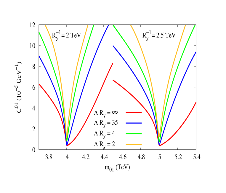
Figure 3: Relic density contours for different values of $R_{y}$ and $\Lambda$. Parameter points above the curves are allowed.

With the graviton in play, an efficient annihilation mode opens up, thereby allowing a much heavier $B^{(1)}$ to be consistent with the relic density than was allowed within mUED (see Fig.3). Understandably, this process is most efficient close to the resonance, which, for the non-relativistic DM particles, would occur when $m_{01}\approx 2M_{B^{(1)}}\sim 2R_{y}^{-1}$. In Fig.3, this is attested to by the severe dip in the size of the required coupling, as is shown by the lowest curve corresponding to the hypothetical case where all SM excitations other than the $B^{(1)}$ have been switched off (or $\Lambda R\to\infty$). The asymmetrical nature of the curve is a result of the interplay of three factors, the natural width of the $h^{(0,1)}$ which grows as the cube of its mass, the fact that the $B^{(1)}$ may have a small but nonzero momentum, and the functional dependence of the annihilation cross sections.

More realistic cases are represented by the other curves in Fig.3. While the salient features remain similar, the increase in the required coupling was expected in view of the discussions above. The dependence of the increase on $\Lambda$ is but a reflection of the fact that a smaller $\Lambda$ implies smaller splittings, and, hence, more states conspiring to increase $n_{B^{(1)}}$. Furthermore, as $m_{01}$ grows sufficiently beyond $2M_{B^{(1)}}$, the graviton is allowed to decay into the other SM KK-excitations as well, thereby ameliorating the asymmetry. For small enough $\Lambda$ and large enough $m_{01}$ this effect clearly overcompensates.

Fig.4 displays the region in the parameter space that satisfies the relic density constraint as well as reproducing $m_{\rm Higgs}=126$ GeV without invoking a substantial little hierarchy ($1>\gamma\mathrel{\hbox to0.0pt{\raise 2.15277pt\hbox{$>$}\hss}{\lower 2.15277pt\hbox{$\sim$}}}0.7$). For a given compactification radius $R_{y}$, the fundamental parameters $k$ and $\epsilon$ are highly correlated, with the latter adopting moderate values consonant with a semiclassical treatment. It is particularly intriguing to note that the fundamental scale in such models is close to the left-right symmetry scale, namely $M_{6}\sim 10^{14}$ GeV (with $r_{z}^{-1}$ being a factor of 20–80 smaller). This is likely to have interesting implications for model building.

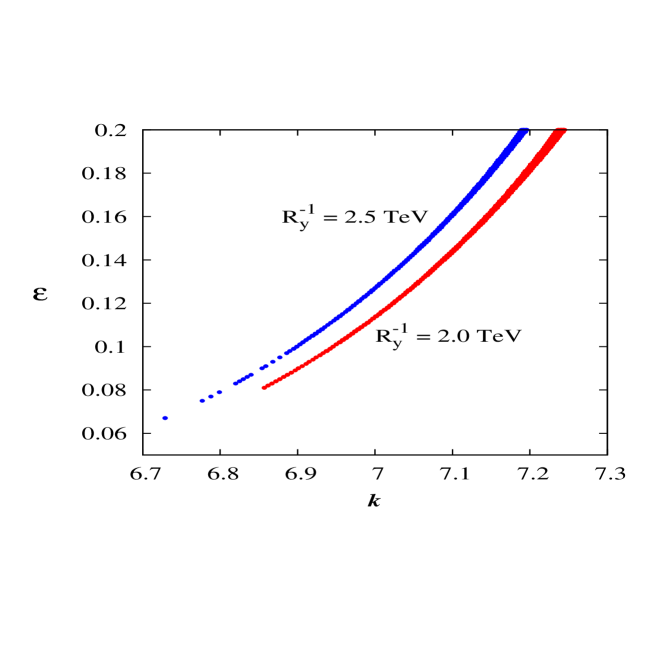
Figure 4: The region in the $k$–$\epsilon$ plane allowed by the relic density for two values of $R_{y}$. Difference between $\Lambda R=4\,(35)$ is invisible on the scale of the graph.

6 Conclusions and Outlook

The generalization of the RS paradigm to nested warping, thus, not only sheds some light on the very scale of the UED paradigm (in turn, related to the mass hierarchy), but also resolves the acute tension between the requirements imposed by the DM relic density on the one hand, and non-observation of the UED excitations at the LHC on the other. While the first issue is not entirely solved, very good reasons exits why the scale of the compactification in the UED direction should be a little below that of the inherent energy scale of the UED brane, which, in turn, is stabilized through the introduction of bulk scalars that provide the requisite effective potentials. The solution to the second (and, phenomenologically, more immediate) problem is much easier to understand. The immersion of the UED-like model in a RS-like warped background (in a higher dimension) provides a new mode for DM-DM annihilation. The consequent dilution in the relic number density allows for heavier DM and, thus, a higher UED scale, thereby allowing one to escape the conflict between LHC observations and the bounds from WMAP/Planck. Simultaneously, this immersion helps us evade the LHC structures against the plain RS scenario. This, essentially, comes about as a consequence of two features. For one, the introduction of a large quasi-UED scale serves to reduce the fundamental scale from $M_{\rm Pl}$ to one that is significantly smaller. Simultaneously, going to the sixth dimension results in quantitatively changing the wavefunction of the corresponding KK-graviton near the IR brane, thereby suppressing its coupling to the brane localized fields. This has the direct consequence of suppressing the single production of the graviton (which would, then, show up in modes such as dileptons, diphotons, dijets etc.). The very same immersion is also the one responsible for the protection of the UED scale.

Given these successes, it is contingent upon us to examine the consistency of this model with other experiments. As for direct detection experiments, the smaller couplings (and at least twice as large a mass) of the gravitons along with the fact that they appear only in the $t$-channel renders their contribution to be vanishingly small. The DM-nucleon scattering cross sections, thus, are very similar to the mUED case, and for the parameter space in Fig.4, explicit calculations (using micrOMEGAs) yield numbers well below the strongest current limits [38].

The situation is much more complex when it comes to indirect detection. The thermal-averaged annihilation cross sections for $B_{1}B_{1}\rightarrow b\bar{b}/W^{+}W^{-}/ZZ/gg$ etc. are several orders of magnitude below the most restrictive limits from AMS-02[39] and Fermi-LAT[40]. On the other hand, the unsuppressed coupling (vis. a vis. other species) of the $B_{1}$ to photons implies a significantly large cross-section for a pair of the DM particles annihilating into a diphoton pair. With the latter being quasi-monochromatic, this would stand out in the sky. Indeed the corresponding rates are very close to the upper limits deduced from H.E.S.S.(consider, for example, Fig.4 of Ref.[41]). In particular, if parameters are such that a pair of a non relativistic DM particles is very close to the graviton resonance, the rate of annihilation could even exceed the limits imposed by H.E.S.S.. For example, consider a situation with $R_{y}^{-1}=2.5\,{\rm TeV}$ and $\Lambda=35$. If we have $m_{01}=5$ TeV (i.e., almost on resonance), this would result in $\langle\sigma v\rangle(B_{1}B_{1}\rightarrow\gamma\gamma)=$6.1$\times$ 10^-27cm${}^{3}/$s, which is larger than what H.E.S.S. allows for. On the other hand, if we had $m_{01}=4.7$ TeV instead, then (even while accounting for the larger coupling required to satisfy the relic density bound), we would have had $\langle\sigma v\rangle(B_{1}B_{1}\rightarrow\gamma\gamma)=$3.6$\times$ 10^-27cm${}^{3}/$s, and, hence, well within the allowed region. Much the same happens for $m_{01}>2\,R_{y}^{-1}$. Several caveats exist, though. For one, the bounds depend very sensitively on the choice for the galactic DM profile; for DM particles as heavy as we consider and the somewhat nonstandard couplings that it has, the uncertainties in the profile are quite significant. Moreover, choosing a moderately large value of $\Lambda R_{y}$ further suppresses such cross sections. It should be noted here that the embedding in the warped dimension essentially removes the stringent constraints on $\Lambda R_{y}$ that were operative in the canonical UED scenario. Nonetheless, this would remain a particularly interesting channel and is the most likely theater for a critical examination of the paradigm. Naively, it might seem that the very same coupling (of the DM to the photon) would lead to severe modification in CMB observations[42] and long-distance observations, such as those of blazars and quasars. However, once again, the scattering of such photons by the intervening DM would need to proceed through $t$-channel graviton exchanges, and given the size of the couplings, are of little concern.

Finally, we comment on the prospects at the LHC. While the presence of the gravitons (particularly, the $h_{01}$), has allowed us the upper limit of $R^{-1}\sim 1400\,{\rm GeV}$ (operative in the canonical minimal UED) from considerations of the relic density, it is not that one can allow of arbitrarily large $R_{y}^{-1}$. As Fig.4 suggests, larger values of $R_{y}^{-1}$ typically require larger $\epsilon$ values, thereby calling into question the semiclassical treatment. Indeed, such considerations restrict one to $R_{y}^{-1}\mathrel{\hbox to0.0pt{\raise 2.15277pt\hbox{$<$}\hss}{\lower 2.15277pt\hbox{$\sim$}}}3.5\,{\rm TeV}$ thereby bringing the model wholly into the reach of the LHC.

References

- [1] WMAP collaboration, E. Komatsu et al., Seven-Year Wilkinson Microwave Anisotropy Probe (WMAP) Observations: Cosmological Interpretation, Astrophys. J. Suppl. 192 (2011) 18, [1001.4538].
- [2] Planck collaboration, P. A. R. Ade et al., Planck 2015 results. XIII. Cosmological parameters, Astron. Astrophys. 594 (2016) A13, [1502.01589].
- [3] I. Antoniadis, A Possible new dimension at a few TeV, Phys. Lett. B246 (1990) 377–384.
- [4] M. Gogberashvili, Hierarchy problem in the shell universe model, Int. J. Mod. Phys. D11 (2002) 1635–1638, [hep-ph/9812296].
- [5] L. Randall and R. Sundrum, A Large mass hierarchy from a small extra dimension, Phys. Rev. Lett. 83 (1999) 3370–3373, [hep-ph/9905221].
- [6] CMS collaboration, V. Khachatryan et al., Search for high-mass diphoton resonances in proton–proton collisions at 13 TeV and combination with 8 TeV search, Phys. Lett. B767 (2017) 147–170, [1609.02507].
- [7] The ATLAS collaboration, Search for resonances in diphoton events with the ATLAS detector at = 13 TeV, Tech. Rep. ATLAS-CONF-2016-018, CERN, Geneva, Mar, 2016.
- [8] H. Davoudiasl, J. L. Hewett and T. G. Rizzo, Phenomenology of the Randall-Sundrum Gauge Hierarchy Model, Phys. Rev. Lett. 84 (2000) 2080, [hep-ph/9909255].
- [9] T. Appelquist, H.-C. Cheng and B. A. Dobrescu, Bounds on universal extra dimensions, Phys. Rev. D64 (2001) 035002, [hep-ph/0012100].
- [10] H.-C. Cheng, K. T. Matchev and M. Schmaltz, Bosonic supersymmetry? Getting fooled at the CERN LHC, Phys. Rev. D66 (2002) 056006, [hep-ph/0205314].
- [11] K. Kong and K. T. Matchev, Precise calculation of the relic density of Kaluza-Klein dark matter in universal extra dimensions, JHEP 01 (2006) 038, [hep-ph/0509119].
- [12] G. Servant and T. M. P. Tait, Is the lightest Kaluza-Klein particle a viable dark matter candidate?, Nucl. Phys. B650 (2003) 391–419, [hep-ph/0206071].
- [13] H.-C. Cheng, J. L. Feng and K. T. Matchev, Kaluza-Klein dark matter, Phys. Rev. Lett. 89 (2002) 211301, [hep-ph/0207125].
- [14] D. Hooper and S. Profumo, Dark matter and collider phenomenology of universal extra dimensions, Phys. Rept. 453 (2007) 29–115, [hep-ph/0701197].
- [15] CMS collaboration, V. Khachatryan et al., Search for dark matter, extra dimensions, and unparticles in monojet events in proton–proton collisions at TeV, Eur. Phys. J. C75 (2015) 235, [1408.3583].
- [16] ATLAS collaboration, G. Aad et al., Search for new phenomena in final states with an energetic jet and large missing transverse momentum in pp collisions at 8 TeV with the ATLAS detector, Eur. Phys. J. C75 (2015) 299, [1502.01518].
- [17] The ATLAS collaboration, Search for squarks and gluinos in final states with jets and missing transverse momentum at =13 TeV with the ATLAS detector, Tech. Rep. ATLAS-CONF-2015-062, CERN, Geneva, 2015.
- [18] CMS collaboration, V. Khachatryan et al., Search for supersymmetry in the multijet and missing transverse momentum final state in pp collisions at 13 TeV, Phys. Lett. B758 (2016) 152–180, [1602.06581].
- [19] D. Choudhury and K. Ghosh, Bounds on Universal Extra Dimension from LHC Run I and II data, Phys. Lett. B763 (2016) 155–160, [1606.04084].
- [20] N. Deutschmann, T. Flacke and J. S. Kim, Current LHC Constraints on Minimal Universal Extra Dimensions, 1702.00410.
- [21] J. Beuria, A. Datta, D. Debnath and K. T. Matchev, LHC Collider Phenomenology of Minimal Universal Extra Dimensions, 1702.00413.
- [22] G. Belanger, M. Kakizaki and A. Pukhov, Dark matter in UED: The Role of the second KK level, JCAP 1102 (2011) 009, [1012.2577].
- [23] S. Chakraborty, S. Niyogi and K. Sridhar, private communication, .
- [24] D. Choudhury and S. SenGupta, Living on the edge in a spacetime with multiple warping, Phys. Rev. D76 (2007) 064030, [hep-th/0612246].
- [25] M. T. Arun and D. Choudhury, Stabilization of moduli in spacetime with nested warping and the UED, Nucl. Phys. B923 (2017) 258–276, [1606.00642].
- [26] S. Alexander, Y. Ling and L. Smolin, A Thermal instability for positive brane cosmological constant in the Randall-Sundrum cosmologies, Phys. Rev. D65 (2002) 083503, [hep-th/0106097].
- [27] M. T. Arun, D. Choudhury, A. Das and S. SenGupta, Graviton modes in multiply warped geometry, Phys. Lett. B746 (2015) 266–275, [1410.5591].
- [28] M. T. Arun and P. Saha, Gravitons in multiply warped scenarios - at 750 GeV and beyond, 1512.06335.
- [29] W. D. Goldberger and M. B. Wise, Modulus stabilization with bulk fields, Phys. Rev. Lett. 83 (1999) 4922–4925, [hep-ph/9907447].
- [30] R. Barbieri and G. F. Giudice, Upper Bounds on Supersymmetric Particle Masses, Nucl. Phys. B306 (1988) 63–76.
- [31] J. R. Ellis, K. Enqvist, D. V. Nanopoulos and F. Zwirner, Observables in Low-Energy Superstring Models, Mod. Phys. Lett. A1 (1986) 57.
- [32] M. T. Arun and D. Choudhury, Bulk gauge and matter fields in nested warping: II. Symmetry Breaking and phenomenological consequences, JHEP 04 (2016) 133, [1601.02321].
- [33] J. M. Cornell, S. Profumo and W. Shepherd, Dark matter in minimal universal extra dimensions with a stable vacuum and the “right” Higgs boson, Phys. Rev. D89 (2014) 056005, [1401.7050].
- [34] A. Datta and S. Raychaudhuri, Vacuum Stability Constraints and LHC Searches for a Model with a Universal Extra Dimension, Phys. Rev. D87 (2013) 035018, [1207.0476].
- [35] G. Belanger, F. Boudjema, A. Pukhov and A. Semenov, MicrOMEGAs 2.0: A Program to calculate the relic density of dark matter in a generic model, Comput. Phys. Commun. 176 (2007) 367–382, [hep-ph/0607059].
- [36] A. Semenov, LanHEP — A package for automatic generation of Feynman rules from the Lagrangian. Version 3.2, Comput. Phys. Commun. 201 (2016) 167–170, [1412.5016].
- [37] A. Belyaev, M. Brown, J. Moreno and C. Papineau, Discovering Minimal Universal Extra Dimensions (MUED) at the LHC, JHEP 06 (2013) 080, [1212.4858].
- [38] LUX collaboration, D. S. Akerib et al., Results from a search for dark matter in the complete LUX exposure, Phys. Rev. Lett. 118 (2017) 021303, [1608.07648].
- [39] S.-J. Lin, X.-J. Bi, P.-F. Yin and Z.-H. Yu, Implications for dark matter annihilation from the AMS-02 ratio, 1504.07230.
- [40] Fermi-LAT collaboration, M. Ackermann et al., Searching for Dark Matter Annihilation from Milky Way Dwarf Spheroidal Galaxies with Six Years of Fermi Large Area Telescope Data, Phys. Rev. Lett. 115 (2015) 231301, [1503.02641].
- [41] H.E.S.S. collaboration, A. Abramowski et al., Search for Photon-Linelike Signatures from Dark Matter Annihilations with H.E.S.S., Phys. Rev. Lett. 110 (2013) 041301, [1301.1173].
- [42] R. J. Wilkinson, J. Lesgourgues and C. Boehm, Using the CMB angular power spectrum to study Dark Matter-photon interactions, JCAP 1404 (2014) 026, [1309.7588].