Abstract

The neutrino $\mu$-$\tau$ reflection symmetry has been attracting a lot of attention as it predicts the interesting results $\theta_{23}=\pi/4$ and $\delta=\pm\pi/2$. But it is reasonable to consider breakings of such a symmetry either from the theoretical considerations or on the basis of experimental results. We thus perform a systematic study for the possible symmetry-breaking patterns and their implications for the mixing parameters. The general treatment is applied to some specific symmetry breaking arising from the renormalization group effects for illustration.

1 Introduction

The discovery of neutrino oscillations indicates that neutrinos are massive and bear flavor mixing. The neutrino mixing arises from the mismatch between their mass and flavor eigenstates, and is described by a $3\times 3$ unitary matrix $U=U^{\dagger}_{l}U_{\nu}$ (with $U_{l}$ and $U_{\nu}$ being respectively the unitary matrix for diagonalizing the charged-lepton mass matrix $M_{l}M^{\dagger}_{l}$ and neutrino mass matrix $M_{\nu}$). In the standard parametrization, $U$ reads

$$U=P_{\phi}\left(\begin{matrix}c_{12}c_{13}&s_{12}c_{13}&s_{13}e^{-{\rm i}\delta}\cr-s_{12}c_{23}-c_{12}s_{23}s_{13}e^{{\rm i}\delta}&c_{12}c_{23}-s_{12}s_{23}s_{13}e^{{\rm i}\delta}&s_{23}c_{13}\cr s_{12}s_{23}-c_{12}c_{23}s_{13}e^{{\rm i}\delta}&-c_{12}s_{23}-s_{12}c_{23}s_{13}e^{{\rm i}\delta}&c_{23}c_{13}\end{matrix}\right)P_{\nu}\;,$$ (1)

where $\theta_{ij}$ (for $ij=12,13,23$) are the mixing angles (with $c_{ij}=\cos{\theta_{ij}}$ and $s_{ij}=\sin{\theta_{ij}}$) and $\delta$ is the Dirac CP phase. $P_{\nu}={\rm Diag}(e^{{\rm i}\rho},e^{{\rm i}\sigma},1)$ contains two Majorana CP phases $\rho$ and $\sigma$, while $P_{\phi}={\rm Diag}(e^{{\rm i}\phi_{1}},e^{{\rm i}\phi_{2}},e^{{\rm i}\phi_{3}})$ consists of three unphysical phases $\phi_{1,2,3}$ that can be removed via the charged-lepton field rephasing. In addition, neutrino oscillations are also controlled by two mass-squared differences $\Delta m^{2}_{ij}=m^{2}_{i}-m^{2}_{j}$ (for $ij=21,31$). Thanks to various neutrino-oscillation experiments [1], the neutrino mixing parameters have been measured to a good accuracy. A global-fit result [2] for them is given by

$$\sin^{2}{\theta_{12}}=0.308\pm 0.017\;,\hskip 45.52458pt\Delta m^{2}_{21}=(7.54\pm 0.24)\times 10^{-5}\ {\rm eV}^{2}\;,$$

$$\sin^{2}{\theta_{13}}=0.0234\pm 0.0020\;,\hskip 28.45274pt|\Delta m^{2}_{31}|=(2.47\pm 0.06)\times 10^{-3}\ {\rm eV}^{2}\;.$$ (2)

Note that the sign of $\Delta m^{2}_{31}$ remains undetermined, allowing for two possible neutrino mass orderings $m_{1}<m_{2}<m_{3}$ (referred to as the normal hierarchy and NH for short) or $m_{3}<m_{1}<m_{2}$ (the inverted hierarchy and IH for short). The absolute neutrino mass scale is not known either, but subject to the constraint $m_{1}+m_{2}+m_{3}<0.23$ eV from cosmological observations [3]. Particularly noteworthy, a recent result from the NOvA experiment ($\theta_{23}=39.5^{\circ}\pm 1.7^{\circ}$ or $52.1^{\circ}\pm 1.7^{\circ}$ in the NH case) disfavors the popular maximal mixing scenario $\theta_{23}=45^{\circ}$ with 2.6$\sigma$ significance [4]. On the other hand, it is interesting to find that the best-fit result for $\delta$ is around $270^{\circ}$ ($261^{\circ}\pm 55^{\circ}$ for NH and $277^{\circ}\pm 43^{\circ}$ for IH) [5].

How to understand the neutrino mixing pattern poses an interesting question. As symmetries (e.g., the $\rm SU(3)_{q}$ quark flavor symmetry) have been serving as a guideline for understanding the particle physics, they may play a similar role in addressing the flavor issues. Along this line, many discrete groups have been proposed as the lepton flavor symmetry [6]. A simplest example is the $\mu$-$\tau$ permutation symmetry [7, 8]: In the basis of $M_{l}$ being diagonal, $M_{\nu}$ should keep unchanged with respect to the transformation $\nu_{\mu}\leftrightarrow\nu_{\tau}$ and thus feature $M_{e\mu}=M_{e\tau}$ and $M_{\mu\mu}=M_{\tau\tau}$ (with $M_{\alpha\beta}$ for $\alpha,\beta=e,\mu,\tau$ being the matrix elements of $M_{\nu}$). Such a symmetry (which results in $\theta_{23}=\pi/4$ and $\theta_{13}=0$) was historically motivated by the experimental facts that $\theta_{23}$ takes a value close to $\pi/4$ while $\theta_{13}$ was only constrained by $\sin^{2}{2\theta_{13}}<0.18$ [9] (and thus might be negligibly small) at the time. However, the relatively large $\theta_{13}\simeq 0.15$ observed recently [10] requires a significant breaking of this symmetry unless neutrinos are quasi-degenerate in masses [11]. Hence we need to go beyond this simple possibility to accommodate the experimental results in a better way. In this connection, the $\mu$-$\tau$ reflection symmetry [12, 8] may serve as a unique alternative: When $M_{l}$ is diagonal, $M_{\nu}$ should remain invariant under the transformation

$$\nu_{e}\leftrightarrow\nu^{c}_{e}\;,\hskip 28.45274pt\nu_{\mu}\leftrightarrow\nu^{c}_{\tau}\;,\hskip 28.45274pt\nu_{\tau}\leftrightarrow\nu^{c}_{\mu}\;,$$ (3)

and thus be characterized by

$$M_{e\mu}=M^{*}_{e\tau}\;,\hskip 28.45274ptM_{\mu\mu}=M^{*}_{\tau\tau}\;,\hskip 28.45274ptM_{ee}=M^{*}_{ee}\;,\hskip 28.45274ptM_{\mu\tau}=M^{*}_{\mu\tau}\;.$$ (4)

In addition to allowing for an arbitrary $\theta_{13}$, this symmetry predicts $\theta_{23}=\pi/4$ and $\delta=\pm\pi/2$ [14] which are close to the present data, thereby having been attracting a lot of interests [15]. Moreover, $\rho$ and $\sigma$ are required to take the trivial values 0 or $\pi/2$.

Nevertheless, it is hard to believe that the $\mu$-$\tau$ reflection symmetry can remain as an exact one. On the experimental side, the aforementioned results seem to hint towards $\theta_{23}\neq\pi/4$ (and possibly $\delta\neq\pm\pi/2$). On the theoretical side, flavor symmetries are generally implemented at a superhigh energy scale and so the renormalization group (RG) running effect may provide a source for the symmetry breaking as we will see. In view of these considerations, it is worthwhile to consider the breaking of this symmetry. In the next section, we perform a systematic study of the possible symmetry-breaking patterns and their implications for the mixing parameters. First of all, we establish an equation set relating the symmetry-breaking parameters in an $M_{\nu}$ of approximate $\mu$-$\tau$ reflection symmetry and the deviations of mixing parameters from their special values taken in the symmetry context. While the numerical results for these equations are analyzed in section 2.1, some analytical approximations will be derived in section 2.2 to explain the corresponding numerical results. In section 2.3 the general treatment is applied to some specific symmetry breaking arising from the RG running effect. Finally, we summarize our main results in section 3.

2 Breaking of the $\mu$-$\tau$ reflection symmetry

Above all, let us define some parameters to characterize the breaking of $\mu$-$\tau$ reflection symmetry. For this purpose, one can introduce the parameters

$$\epsilon_{1}=\displaystyle\frac{M_{e\mu}-M^{*}_{e\tau}}{M_{e\mu}+M^{*}_{e\tau}}\;,\hskip 28.45274pt\epsilon_{2}=\displaystyle\frac{M_{\mu\mu}-M^{*}_{\tau\tau}}{M_{\mu\mu}+M^{*}_{\tau\tau}}\;,\hskip 28.45274pt\epsilon_{3}=\displaystyle\frac{{\rm Im}(M_{ee})}{{\rm Re}(M_{ee})}\;,\hskip 28.45274pt\epsilon_{4}=\displaystyle\frac{{\rm Im}(M_{\mu\tau})}{{\rm Re}(M_{\mu\tau})}\;,$$ (5)

by following the discussions about the breaking of $\mu$-$\tau$ permutation symmetry in Ref. [16]. Note that they correspond to the four symmetry conditions in Eq. (4) one by one. These parameters have to be small in magnitude (say $|\epsilon_{i}|\leq 0.1$ for $i=1,2,3,4$) in order to keep the $\mu$-$\tau$ reflection symmetry as an approximate one. In terms of them, the most general neutrino mass matrix of an approximate $\mu$-$\tau$ reflection symmetry can always be parameterized in a manner as follows: Suppose, at the symmetry level, there is a neutrino mass matrix of the form

$$M^{(0)}_{\nu}=\left(\begin{matrix}A_{0}&\hskip 8.5359ptB_{0}&\hskip 8.5359ptB^{*}_{0}\cr B_{0}&\hskip 8.5359ptC_{0}&\hskip 8.5359ptD_{0}\cr B^{*}_{0}&\hskip 8.5359ptD_{0}&\hskip 8.5359ptC^{*}_{0}\end{matrix}\right)\;,$$ (6)

in which $A_{0}$ and $D_{0}$ are real. This neutrino mass matrix can be diagonalized by a unitary matrix $U^{(0)}$ (an analogue of $U$) with its parameters satisfying the requirements

$$\phi^{(0)}_{1}=\phi^{(0)}_{2}+\phi^{(0)}_{3}=0\;,\hskip 28.45274pt\theta^{(0)}_{23}=\pi/4\;,\hskip 28.45274pt\delta^{(0)}=\pm\pi/2\;,\hskip 28.45274pt\rho^{(0)},\sigma^{(0)}=0\;\;{\rm or}\;\;\pi/2\;.$$ (7)

After the symmetry is softly broken, $M^{(0)}_{\nu}$ may receive a general perturbation as given by

$$M^{(1)}_{\nu}=\left(\begin{matrix}\delta_{ee}&\hskip 8.5359pt\delta_{e\mu}&\hskip 8.5359pt\delta_{e\tau}\cr\delta_{e\mu}&\hskip 8.5359pt\delta_{\mu\mu}&\hskip 8.5359pt\delta_{\mu\tau}\cr\delta_{e\tau}&\hskip 8.5359pt\delta_{\mu\tau}&\hskip 8.5359pt\delta_{\tau\tau}\end{matrix}\right)\;,$$ (8)

which can be decomposed into two parts as

$$M^{(1)}_{\nu}=\frac{1}{2}\left(\begin{matrix}2{\rm Re}(\delta_{ee})&\hskip 8.5359pt\delta_{e\mu}+\delta^{*}_{e\tau}&\hskip 8.5359pt\delta^{*}_{e\mu}+\delta_{e\tau}\cr\delta_{e\mu}+\delta^{*}_{e\tau}&\hskip 8.5359pt\delta_{\mu\mu}+\delta^{*}_{\tau\tau}&\hskip 8.5359pt2{\rm Re}(\delta_{\mu\tau})\cr\delta^{*}_{e\mu}+\delta_{e\tau}&\hskip 8.5359pt2{\rm Re}(\delta_{\mu\tau})&\hskip 8.5359pt\delta^{*}_{\mu\mu}+\delta_{\tau\tau}\end{matrix}\right)+\frac{1}{2}\left(\begin{matrix}2{\rm iIm}(\delta_{ee})&\hskip 8.5359pt\delta_{e\mu}-\delta^{*}_{e\tau}&\hskip 8.5359pt\delta_{e\tau}-\delta^{*}_{e\mu}\cr\delta_{e\mu}-\delta^{*}_{e\tau}&\hskip 8.5359pt\delta_{\mu\mu}-\delta^{*}_{\tau\tau}&\hskip 8.5359pt2{\rm iIm}(\delta_{\mu\tau})\cr\delta_{e\tau}-\delta^{*}_{e\mu}&\hskip 8.5359pt2{\rm iIm}(\delta_{\mu\tau})&\hskip 8.5359pt\delta_{\tau\tau}-\delta^{*}_{\mu\mu}\end{matrix}\right)\;.$$ (9)

Consequently, the complete neutrino mass matrix $M_{\nu}=M^{(0)}_{\nu}+M^{(1)}_{\nu}$ can be parameterized as

$$M_{\nu}=\left(\begin{matrix}A(1+{\rm i}\epsilon_{3})&\hskip 8.5359ptB(1+\epsilon_{1})&\hskip 8.5359ptB^{*}(1-\epsilon^{*}_{1})\cr B(1+\epsilon_{1})&\hskip 8.5359ptC(1+\epsilon_{2})&\hskip 8.5359ptD(1+{\rm i}\epsilon_{4})\cr B^{*}(1-\epsilon^{*}_{1})&\hskip 8.5359ptD(1+{\rm i}\epsilon_{4})&\hskip 8.5359ptC^{*}(1-\epsilon^{*}_{2})\end{matrix}\right)\;,$$ (10)

with

$$A=A_{0}+{\rm Re}(\delta_{ee})\;,\hskip 22.76228pt B=B_{0}+\displaystyle\frac{\delta_{e\mu}+\delta^{*}_{e\tau}}{2}\;,$$ (11)

$$D=D_{0}+{\rm Re}(\delta_{\mu\tau})\;,\hskip 22.76228pt C=C_{0}+\displaystyle\frac{\delta_{\mu\mu}+\delta^{*}_{\tau\tau}}{2}\;,$$

and

$$\epsilon_{1}=\frac{\delta_{e\mu}-\delta^{*}_{e\tau}}{2B}\;,\hskip 28.45274pt\epsilon_{2}=\frac{\delta_{\mu\mu}-\delta^{*}_{\tau\tau}}{2C}\;,\hskip 28.45274pt\epsilon_{3}=\frac{{\rm Im}(\delta_{ee})}{A}\;,\hskip 28.45274pt\epsilon_{4}=\frac{{\rm Im}(\delta_{\mu\tau})}{D}\;.$$ (12)

It should be noted that ${\rm Im}(\epsilon_{1,2})$ and $\epsilon_{3,4}$ will transform in a way as

$${\rm Im}(\epsilon_{1})\to{\rm Im}(\epsilon_{1})+\varphi_{1}+(\varphi_{2}+\varphi_{3})/2\;,\hskip 28.45274pt\epsilon_{3}\to\epsilon_{3}+2\varphi_{1}\;,$$

$${\rm Im}(\epsilon_{2})\to{\rm Im}(\epsilon_{2})+\varphi_{2}+\varphi_{3}\;,\hskip 28.45274pt\epsilon_{4}\to\epsilon_{4}+\varphi_{2}+\varphi_{3}\;,$$ (13)

under the neutrino-field rephasing

$$\nu_{e}\to e^{{\rm i}\varphi_{1}}\nu_{e}\simeq(1+{\rm i}\varphi_{1})\nu_{e}\;,\hskip 28.45274pt\nu_{\mu}\to e^{{\rm i}\varphi_{2}}\nu_{\mu}\simeq(1+{\rm i}\varphi_{2})\nu_{\mu}\;,$$

$$\nu_{\tau}\to e^{{\rm i}\varphi_{3}}\nu_{\tau}\simeq(1+{\rm i}\varphi_{3})\nu_{\tau}\;,$$ (14)

with $\varphi_{1,2,3}$ being some small parameters comparable to $\epsilon_{i}$. Taking advantage of such a freedom, one can always achieve $\epsilon_{3,4}=0$ from the general case given by Eq. (10). In the following discussions, we therefore concentrate on this particular case without loss of generality.

Starting from an $M_{\nu}$ of the form in Eq. (10) but with $\epsilon_{3,4}=0$, we study dependence of the mixing parameters on $\epsilon_{1,2}$. To this end, we diagonalize such an $M_{\nu}$ with one unitary matrix in a straightforward way

$$U^{\dagger}M_{\nu}U^{*}={\rm Diag}(m_{1},m_{2},m_{3})\;.$$ (15)

The mixing parameters in $U$ are expected to lie around those special values in Eq. (7) and the corresponding deviations

$$\Delta\phi_{1}=\phi_{1}-0\;, \hskip 28.45274pt\Delta\phi=(\phi_{2}+\phi_{3})/2-0\;, \hskip 28.45274pt\Delta\theta=\theta_{23}-\pi/4\;,$$

$$\Delta\delta=\delta-\delta^{(0)}\;, \Delta\rho=\rho-\rho^{(0)}\;, \hskip 28.45274pt\Delta\sigma=\sigma-\sigma^{(0)}\;,$$ (16)

are some small quantities. By making perturbation expansions for these small quantities in Eq. (15), one reaches the following relations that connect the mixing-parameter deviations with $\epsilon_{1,2}$

$$m_{3}s^{2}_{13}\Delta\delta+\overline{m}_{1}c^{2}_{12}\Delta\rho+\overline{m}_{2}s^{2}_{12}\Delta\sigma=(m_{3}s^{2}_{13}-m_{11})\Delta\phi_{1}\;,$$

$$2m_{12}\bar{s}_{13}\Delta\theta-m_{11}s^{2}_{13}\Delta\delta-\overline{m}_{1}s^{2}_{12}\Delta\rho-\overline{m}_{2}c^{2}_{12}\Delta\sigma=(m_{22}-m_{3})\Delta\phi\;,$$

$$[m_{12}+{\rm i}(m_{11}+m_{3})\bar{s}_{13}]\Delta\theta-(m_{11}-m_{3})\bar{s}_{13}\Delta\delta-2\overline{m}_{1}c_{12}({\rm i}s_{12}+c_{12}\bar{s}_{13})\Delta\rho$$

$$\hskip 19.91684pt+2\overline{m}_{2}s_{12}({\rm i}c_{12}-s_{12}\bar{s}_{13})\Delta\sigma=[m_{12}-{\rm i}(m_{11}+m_{3})\bar{s}_{13}]({\rm i}\Delta\phi_{1}+{\rm i}\Delta\phi-\epsilon_{1})\;,$$

$$2(m_{22}-m_{3})\Delta\theta-2(m_{12}-{\rm i}m_{11}\bar{s}_{13})\bar{s}_{13}\Delta\delta-2\overline{m}_{1}s_{12}({\rm i}s_{12}+2c_{12}\bar{s}_{13})\Delta\rho$$

$$\hskip 19.91684pt-2\overline{m}_{2}c_{12}({\rm i}c_{12}-2s_{12}\bar{s}_{13})\Delta\sigma=(m_{22}+m_{3}-2{\rm i}m_{12}\bar{s}_{13})(2{\rm i}\Delta\phi-\epsilon_{2})\;.$$ (17)

In order to make the expressions compact, the definitions

$$m_{11}=\overline{m}_{1}c^{2}_{12}+\overline{m}_{2}s^{2}_{12}\;,\hskip 28.45274ptm_{12}=(\overline{m}_{1}-\overline{m}_{2})c_{12}s_{12}\;,\hskip 28.45274ptm_{22}=\overline{m}_{1}s^{2}_{12}+\overline{m}_{2}c^{2}_{12}\;,$$

$$\overline{m}_{1}=m_{1}{\rm exp}[2{\rm i}\rho^{(0)}]\;,\hskip 41.25641pt\overline{m}_{2}=m_{2}{\rm exp}[2{\rm i}\sigma^{(0)}]\;,\hskip 46.94687pt\bar{s}_{13}=-{\rm i}s_{13}{\rm exp}[{\rm i}\delta^{(0)}]\;,$$ (18)

have been taken.

After solving Eq. (17) we obtain $\Delta\theta$, $\Delta\delta$, $\Delta\rho$ and $\Delta\sigma$ as some linear functions of ${\rm R}_{1,2}={\rm Re}(\epsilon_{1,2})$ and ${\rm I}_{1,2}={\rm Im}(\epsilon_{1,2})$, which can be parameterized as

$$\Delta\theta=c^{\theta}_{r1}{\rm R}_{1}+c^{\theta}_{i1}{\rm I}_{1}+c^{\theta}_{r2}{\rm R}_{2}+c^{\theta}_{i2}{\rm I}_{2}\;,\hskip 28.45274pt \Delta\delta=c^{\delta}_{r1}{\rm R}_{1}+c^{\delta}_{i1}{\rm I}_{1}+c^{\delta}_{r2}{\rm R}_{2}+c^{\delta}_{i2}{\rm I}_{2}\;,$$ (19)

$$\Delta\rho=c^{\rho}_{r1}{\rm R}_{1}+c^{\rho}_{i1}{\rm I}_{1}+c^{\rho}_{r2}{\rm R}_{2}+c^{\rho}_{i2}{\rm I}_{2}\;,\hskip 28.45274pt \Delta\sigma=c^{\sigma}_{r1}{\rm R}_{1}+c^{\sigma}_{i1}{\rm I}_{1}+c^{\sigma}_{r2}{\rm R}_{2}+c^{\sigma}_{i2}{\rm I}_{2}\;.$$

The coefficients in these expressions measure the sensitive strengths of mixing-parameter deviations to the symmetry-breaking parameters. For example, $c^{\theta}_{r1}$ measures the sensitive strength of $\Delta\theta$ to ${\rm R}_{1}$. The contribution of any given ${\rm R}_{1}$ to $\Delta\theta$ is expressed as the product of it with $c^{\theta}_{r1}$ (i.e., $c^{\theta}_{r1}{\rm R}_{1}$). There are two things to be noted: For one thing, such a ${\rm R}_{1}$ will also contribute to $\Delta\delta$, $\Delta\rho$ and $\Delta\sigma$ by an amount of $c^{\delta}_{r1}{\rm R}_{1}$, $c^{\rho}_{r1}{\rm R}_{1}$ and $c^{\sigma}_{r1}{\rm R}_{1}$, respectively. For another thing, $\Delta\theta$ would receive an additional contribution of $c^{\theta}_{i1}{\rm I}_{1}$ ($c^{\theta}_{r2}{\rm R}_{2}$ or $c^{\theta}_{i2}{\rm I}_{2}$) if ${\rm I}_{1}$ (${\rm R}_{2}$ or ${\rm I}_{2}$) were non-vanishing in the meanwhile. In consideration of the pre-requisition $|\epsilon_{1,2}|\leq 0.1$, the coefficients must have magnitudes $\geq\mathcal{O}(1)$ in order to cause some sizeable (say $0.1\simeq 6^{\circ}$) mixing-parameter deviations. If one coefficient is much greater than 1 (say 10 or 100), even a tiny (at least 0.01 or 0.001) symmetry-breaking parameter can give rise to some sizable mixing-parameter deviation. But if one coefficient is much smaller than 1 (say 0.1 or 0.01), the resulting mixing-parameter deviation will be negligibly small (at most 0.01 or 0.001). Although the mixing-parameter deviations are of direct interest, we will first concentrate on the coefficients and then turn to their implications for the mixing-parameter deviations for the following considerations: (1) Given any specific symmetry-breaking pattern (i.e., definite ${\rm R}_{1,2}$ and ${\rm I}_{1,2}$) in some physical context (e.g., the RG-induced symmetry breaking as will be discussed in section 2.3), the resulting mixing-parameter deviations can be read directly by making use of Eq. (19) provided that the coefficients are known. (2) When the mixing-parameters are determined experimentally to a good degree of accuracy, the required symmetry-breaking pattern may be inferred with the help of Eq. (19) provided that the coefficients are known. As one will see, the values of the coefficients (equivalently the mixing-parameter deviations) are strongly correlated with the neutrino mass spectrum and the values of $\rho^{(0)}$ and $\sigma^{(0)}$ once the symmetry-breaking strengths (i.e., the values of ${\rm R}_{1,2}$ and ${\rm I}_{1,2}$) are specified. In the following, this kind of correlations will be studied in some detail both numerically and analytically.

2.1 Numerical results

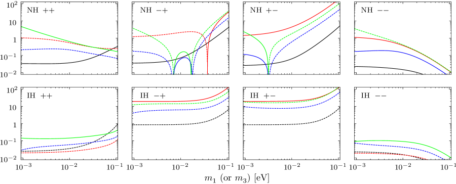
Figure 1: The coefficients associated with ${\rm R_{1}}$ ($c^{\theta}_{r1}$ in black, $c^{\delta}_{r1}$ in red, $c^{\rho}_{r1}$ in green and $c^{\sigma}_{r1}$ in blue) against the lightest neutrino mass $m_{1}$ (or $m_{3}$) in the NH (or IH) case for various combinations of $\rho^{(0)}$ and $\sigma^{(0)}$ with $\delta^{(0)}=-\pi/2$. The signs $++,-+,+-$ and $++$ respectively stand for $[\rho^{(0)},\sigma^{(0)}]=[0,0],[\pi/2,0],[0,\pi/2]$ and $[\pi/2,\pi/2]$.

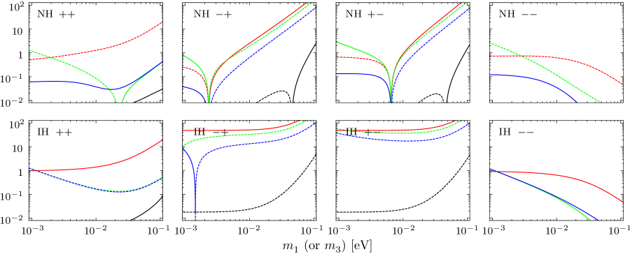
Figure 2: The coefficients associated with ${\rm I_{1}}$ ($c^{\theta}_{i1}$ in black, $c^{\delta}_{i1}$ in red, $c^{\rho}_{i1}$ in green and $c^{\sigma}_{i1}$ in blue) against the lightest neutrino mass $m_{1}$ (or $m_{3}$) in the NH (or IH) case for various combinations of $\rho^{(0)}$ and $\sigma^{(0)}$ with $\delta^{(0)}=-\pi/2$. The signs $++,-+,+-$ and $++$ respectively stand for $[\rho^{(0)},\sigma^{(0)}]=[0,0],[\pi/2,0],[0,\pi/2]$ and $[\pi/2,\pi/2]$.

In this section, the coefficients are explored in a numerical way. In Figs. (1-4) we have presented the coefficients (associated with ${\rm R}_{1}$, ${\rm I}_{1}$, ${\rm R}_{2}$ and ${\rm I}_{2}$ successively) against the lightest neutrino mass ($m_{1}$ for NH or $m_{3}$ for IH) for various combinations of $\rho^{(0)}$ and $\sigma^{(0)}$ (i.e., $[\rho^{(0)},\sigma^{(0)}]=[0,0]$, $[\pi/2,0]$, $[0,\pi/2]$ or $[\pi/2,\pi/2]$). The black, red, green and blue colors are assigned to the coefficients for $\Delta\theta$, $\Delta\delta$, $\Delta\rho$ and $\Delta\sigma$, respectively. In order to save space, the absolute value of a coefficient will be shown in the dashed line if it is negative. By contrast, the full line will be used when the coefficients are positive. As no observable mixing-parameter deviation will arise from a highly suppressed coefficient, the region where the coefficients have magnitudes smaller than 0.01 is not shown. In doing the calculations we have specified $\delta^{(0)}=-\pi/2$. When it takes the opposite value $\pi/2$, the coefficients will either simply stay invariant or just change their signs

$$c^{\theta}_{r1}\to c^{\theta}_{r1}\;,\hskip 34.14322ptc^{\delta}_{r1}\to-c^{\delta}_{r1}\;,\hskip 28.45274ptc^{\rho}_{r1}\to-c^{\rho}_{r1}\;,\hskip 28.45274ptc^{\sigma}_{r1}\to-c^{\sigma}_{r1}\;,$$

$$c^{\theta}_{i1}\to-c^{\theta}_{i1}\;,\hskip 28.45274ptc^{\delta}_{i1}\to c^{\delta}_{i1}\;,\hskip 38.98013ptc^{\rho}_{i1}\to c^{\rho}_{i1}\;,\hskip 39.83368ptc^{\sigma}_{i1}\to c^{\sigma}_{i1}\;,$$

$$c^{\theta}_{r2}\to c^{\theta}_{r2}\;,\hskip 34.14322ptc^{\delta}_{r2}\to-c^{\delta}_{r2}\;,\hskip 28.45274ptc^{\rho}_{r2}\to-c^{\rho}_{r2}\;,\hskip 28.45274ptc^{\sigma}_{r2}\to-c^{\sigma}_{r2}\;,$$

$$c^{\theta}_{i2}\to-c^{\theta}_{i2}\;,\hskip 28.45274ptc^{\delta}_{i2}\to c^{\delta}_{i2}\;,\hskip 38.98013ptc^{\rho}_{i2}\to c^{\rho}_{i2}\;,\hskip 39.83368ptc^{\sigma}_{i2}\to c^{\sigma}_{i2}\;.$$ (20)

The point is that Eq. (17) is invariant with respect to the transformations

$$\Delta\theta\to\Delta\theta\;,\hskip 28.45274pt\Delta\delta\to-\Delta\delta\;,\hskip 28.45274pt\Delta\rho\to-\Delta\rho\;,\hskip 28.45274pt\Delta\sigma\to-\Delta\sigma\;,$$

$${\rm R}_{1}\to{\rm R}_{1}\;,\hskip 32.72049pt{\rm I}_{1}\to-{\rm I}_{1}\;,\hskip 39.83368pt{\rm R}_{2}\to{\rm R}_{2}\;,\hskip 41.25641pt{\rm I}_{2}\to-{\rm I}_{2}\;,$$ (21)

combined with $\bar{s}_{13}\to-\bar{s}_{13}$ as well as $\Delta\phi_{1}\to-\Delta\phi_{1}$ and $\Delta\phi\to-\Delta\phi$. For reference, in Tables (1-4) we have listed some representative values of the coefficients (for $\Delta\theta$, $\Delta\delta$, $\Delta\rho$ and $\Delta\sigma$ successively) at $m_{1}(m_{3})=0.001,0.01$ and 0.1 eV for the NH (IH) case. Numbers in the square brackets denote the coefficients’ values in the IH case. When a coefficient takes values in the range $-0.01\to 0$ or $0\to 0.01$, its values will be reported as 0.00 or $-0.00$.

By virtue of the above numerical results one may draw the following conclusions regarding the coefficients: (1) For $\rho^{(0)}\neq\sigma^{(0)}$ (or $[\rho^{(0)},\sigma^{(0)}]=[\pi/2,\pi/2]$), the coefficients get greatly enhanced (or suppressed) when the neutrino masses are quasi-degenerate $m_{1}\simeq m_{2}\simeq m_{3}$ (e.g., the particular case of $m_{1}(m_{3})\simeq 0.1$ eV). (2) When the absolute neutrino mass scale is small (e.g., the particular case of $m_{1}(m_{3})\simeq 0.001$ eV) and $\rho^{(0)}\neq\sigma^{(0)}$, most of the coefficients will have a much greater magnitude in the IH case compared to in the NH case. (3) $\Delta\theta$ is most sensitive to ${\rm R}_{2}$ while $\Delta\delta$, $\Delta\rho$ and $\Delta\sigma$ to all the symmetry-breaking parameters. In magnitude, the coefficients for $\Delta\delta$, $\Delta\rho$ and $\Delta\sigma$ (which can even obtain some magnitudes around 100 when the neutrino masses are quasi-degenerate and $\rho^{(0)}\neq\sigma^{(0)}$) are generally much greater than those for $\Delta\theta$. Besides these general features, some specific comments for the coefficients are given in order:

1. Among the coefficients for $\Delta\theta$, $|c^{\theta}_{r2}|$ is the most significant one and takes values of $\mathcal{O}$(1) in most cases. But it decreases to $\mathcal{O}$(0.1) in the case of $m_{3}\ll m_{1}\simeq m_{2}$ (e.g., the particular case of $m_{3}\simeq 0.001$ eV) combined with $\rho^{(0)}\neq\sigma^{(0)}$. $|c^{\theta}_{r1}|$ can also reach $\mathcal{O}$(1) in the case of IH combined with $\rho^{(0)}\neq\sigma^{(0)}$. $|c^{\theta}_{i1}|$ and $|c^{\theta}_{i2}|$ are well below $\mathcal{O}$(0.1), indicating that $\Delta\theta$ is insensitive to ${\rm I}_{1,2}$.

2. As for the coefficients for $\Delta\delta$, $|c^{\delta}_{r1}|$ (except in the case of IH combined with $\rho^{(0)}=\sigma^{(0)}$), $|c^{\delta}_{i1}|$ and $|c^{\delta}_{i2}|$ generally have values of $\mathcal{O}$(1) or greater. $|c^{\delta}_{r2}|$ can be significant only in the case of IH combined with $\rho^{(0)}\neq\sigma^{(0)}$.

3. The coefficients for $\Delta\rho$ obtain magnitudes of $\mathcal{O}$(1) or greater in most cases, with the exceptions: $|c^{\rho}_{r1}|$ and $|c^{\rho}_{r2}|$ are substantially suppressed in the case of IH combined with $\rho^{(0)}=\sigma^{(0)}$. The coefficients for $\Delta\sigma$ almost share the same properties as their counterparts for $\Delta\rho$ except that their magnitudes are somewhat smaller (as a result of $m_{2}>m_{1}$).

Now that the coefficients are known well, we discuss their implications for $\Delta\theta$ and $\Delta\delta$ (which are of more practical interests than $\Delta\rho$ and $\Delta\sigma$ since the Majorana phases cannot be pinned down in a foreseeable future).

1. In the case of $m_{3}\ll m_{1}\simeq m_{2}$ (or $m_{1}\simeq m_{2}\simeq m_{3}$) combined with $\rho^{(0)}\neq\sigma^{(0)}$, $|{\rm R}_{1}|\simeq 0.1$ (or $\simeq 0.02$) is capable of producing $|\Delta\theta|\simeq 0.1$. In other cases, $|{\rm R}_{1}|\leq 0.1$ is unable to induce sizable $\Delta\theta$. On the other hand, $|{\rm R}_{2}|\leq 0.1$ can give rise to sizable $\Delta\theta$ in most cases: If the neutrino masses are quasi-degenerate, $|\Delta\theta|\simeq 0.1$ may easily arise (except in the case of $[\rho^{(0)},\sigma^{(0)}]=[\pi/2,\pi/2]$); If not, $|{\rm R}_{2}|\simeq 0.1$ will yield $|\Delta\theta|$ around 0.05 (except in the case of IH combined with $\rho^{(0)}\neq\sigma^{(0)}$). It should be noted that a positive ${\rm R}_{1}$ or ${\rm R}_{2}$ always contributes a positive (or negative) $\Delta\theta$ in the NH (or IH) case. In comparison, $|{\rm I}_{1}|\leq 0.1$ and $|{\rm I}_{2}|\leq 0.1$ cannot lead to sizable $\Delta\theta$ unless the neutrino masses are quasi-degenerate and $\rho^{(0)}\neq\sigma^{(0)}$.

2. For $m_{1}\ll m_{2}\ll m_{3}$ (e.g., the particular case of $m_{1}\simeq 0.001$ eV), $|{\rm R}_{1}|\simeq 0.1$ leads $|\Delta\delta|$ close to 0.1. In the case of $m_{3}\ll m_{1}\simeq m_{2}$ (or $m_{1}\simeq m_{2}\simeq m_{3}$) combined with $\rho^{(0)}\neq\sigma^{(0)}$, sizable $\Delta\delta$ can arise from $|{\rm R}_{1}|$ or $|{\rm R}_{2}|$ as small as 0.01 (or 0.001). In other cases, $|{\rm R}_{1}|\leq 0.1$ and $|{\rm R}_{2}|\leq 0.1$ have no chance to generate sizable $\Delta\delta$. In the $m_{1}\ll m_{2}\ll m_{3}$ case, $|{\rm I}_{1}|\simeq 0.1$ brings about $|\Delta\delta|$ around 0.05. For $m_{3}\ll m_{1}\simeq m_{2}$, $|{\rm I}_{1}|$ as small as 0.01 (or 0.001) may trigger sizable $\Delta\delta$ in the case of $\rho^{(0)}=\sigma^{(0)}$ (or $\rho^{(0)}\neq\sigma^{(0)}$). When the neutrino masses are quasi-degenerate, even a tiny ${\rm I}_{1}$ is able to induce sizable $\Delta\delta$ (except in the case of $[\rho^{(0)},\sigma^{(0)}]=[\pi/2,\pi/2]$). The contributions of ${\rm I}_{2}$ to $\Delta\delta$ bear many similarities with those of ${\rm I}_{1}$.

For illustration, we give a toy example to show how to make use of the above results. In this connection, we discuss how the global-fit results $\theta_{23}/^{\circ}=41.6^{+1.5}_{-1.2}$ and $\delta/^{\circ}=261^{+51}_{-59}$ in the NH case [5] may arise from an approximate $\mu$-$\tau$ reflection symmetry. (For simplicity, only the best-fit results will be used.) Since $\Delta\theta$ is most sensitive to ${\rm R}_{2}$, one wonders whether a single ${\rm R}_{2}$ can give rise to appropriate $\Delta\theta$ and $\Delta\delta$ simultaneously. This requires $c^{\delta}_{r2}/c^{\theta}_{r2}=\Delta\delta/\Delta\theta=(-9^{\circ})/(-3.4^{\circ})\simeq 2.65$. With the aid of Fig. 3, it turns out that the coefficients have chance to fulfill such a requirement in the case of $[\rho^{(0)},\sigma^{(0)}]=[\pi/2,0]$ (see the sub-figure labelled by “NH $-$+”): At $m_{1}=0.019$ eV, the values of $c^{\theta}_{r2}$, $c^{\delta}_{r2}$, $c^{\rho}_{r2}$ and $c^{\sigma}_{r2}$ respectively read 0.78, 2.07, $-$2.45 and $-$0.90. In this case, a ${\rm R}_{2}\simeq-0.076$ will result in $\theta_{23}\simeq 41.6^{\circ}$ and $\delta=261^{\circ}$ (as well as $\rho\simeq 100.7^{\circ}$ and $\sigma\simeq 3.9^{\circ}$).

Finally, we discuss the consequences of breaking of $\mu$-$\tau$ reflection symmetry on the allowed range of effective Majorana neutrino mass $|M_{ee}|$ which directly controls the rates of neutrinoless double-beta decays [17]. For this purpose, one obtains

$${\rm Re}(M_{ee}) \simeq \overline{m}_{1}c^{2}_{12}c^{2}_{13}+\overline{m}_{2}s^{2}_{12}c^{2}_{13}-m_{3}s^{2}_{13}\;,$$

$${\rm Im}(M_{ee}) \simeq \overline{m}_{1}c^{2}_{12}\Delta\rho+\overline{m}_{2}s^{2}_{12}\Delta\sigma+m_{3}s^{2}_{13}\Delta\delta+(m_{11}-m_{3}s^{2}_{13})\Delta\phi_{1}\;.$$ (22)

Because the symmetry-breaking parameter $\epsilon_{3}={\rm Im}(M_{ee})/{\rm Re}(M_{ee})$ should be a small quantity (e.g., $|\epsilon_{3}|\leq 0.1$) if we want to maintain the $\mu$-$\tau$ reflection symmetry as an approximate one, the value of

$$|M_{ee}|=\sqrt{[{\rm Re}(M_{ee})]^{2}+[{\rm Im}(M_{ee})]^{2}}\simeq|{\rm Re}(M_{ee})|\left(1+\frac{\epsilon^{2}_{3}}{2}\right)\;,$$ (23)

can be well approximated by that of $|{\rm Re}(M_{ee})|$. It is thus fair to say that the consequences of breaking of $\mu$-$\tau$ reflection symmetry on the allowed range of $|M_{ee}|$ are negligibly small. In Fig. 5 we present the possible values of $|{\rm Re}(M_{ee})|$ as a function of the lightest neutrino mass $m_{1}$ (or $m_{3}$) in the NH (or IH) case for various combinations of $\rho^{(0)}$ and $\sigma^{(0)}$ [18]. (1) In the NH case, the three components of $|{\rm Re}(M_{ee})|$ add constructively to a maximal level for $[\rho^{(0)},\sigma^{(0)}]=[\pi/2,\pi/2]$. By contrast, the three components will cancel each other out (i.e., $|{\rm Re}(M_{ee})|\simeq 0$) at $m_{1}\simeq 0.002$ eV (or 0.007 eV) for $[\rho^{(0)},\sigma^{(0)}]=[\pi/2,0]$ (or $[0,\pi/2]$). (2) In the IH case, the value of $|{\rm Re}(M_{ee})|$ is mainly determined by the first two components as the third one is highly suppressed. Because of $m_{1}\simeq m_{2}$ in the IH case, $|{\rm Re}(M_{ee})|$ approximates to $m_{1}$ (or $m_{1}(c^{2}_{12}-s^{2}_{12})$) for $\rho^{(0)}=\sigma^{(0)}$ (or $\rho^{(0)}\neq\sigma^{(0)}$).

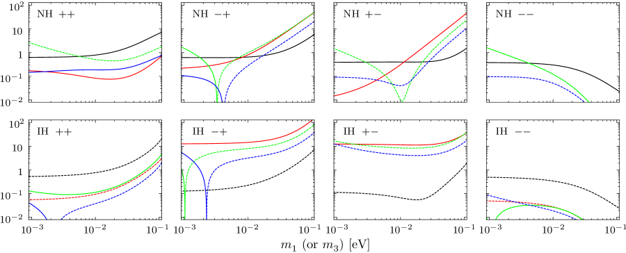
Figure 3: The coefficients associated with ${\rm R_{2}}$ ($c^{\theta}_{r2}$ in black, $c^{\delta}_{r2}$ in red, $c^{\rho}_{r2}$ in green and $c^{\sigma}_{r2}$ in blue) against the lightest neutrino mass $m_{1}$ (or $m_{3}$) in the NH (or IH) case for various combinations of $\rho^{(0)}$ and $\sigma^{(0)}$ with $\delta^{(0)}=-\pi/2$. The signs $++,-+,+-$ and $++$ respectively stand for $[\rho^{(0)},\sigma^{(0)}]=[0,0],[\pi/2,0],[0,\pi/2]$ and $[\pi/2,\pi/2]$.

Figure 4: The coefficients associated with ${\rm I_{2}}$ ($c^{\theta}_{i2}$ in black, $c^{\delta}_{i2}$ in red, $c^{\rho}_{i2}$ in green and $c^{\sigma}_{i2}$ in blue) against the lightest neutrino mass $m_{1}$ (or $m_{3}$) in the NH (or IH) case for various combinations of $\rho^{(0)}$ and $\sigma^{(0)}$ with $\delta^{(0)}=-\pi/2$. The signs $++,-+,+-$ and $++$ respectively stand for $[\rho^{(0)},\sigma^{(0)}]=[0,0],[\pi/2,0],[0,\pi/2]$ and $[\pi/2,\pi/2]$.

		0.001 eV	$0.01$ eV	$0.1$ eV
$[0,0]$	$c^{\theta}_{r1}$	0.03 [$-$0.02]	0.04 [$-$0.04]	0.30 [$-$0.71]
$[\pi/2,0]$		0.04 [$-$0.86]	0.07 [$-$0.89]	3.64 [$-$5.59]
$[0,\pi/2]$		0.03 [$-$0.86]	0.06 [$-$0.91]	4.27 [$-$6.95]
$[\pi/2,\pi/2]$		0.02 [$-$0.02]	0.02 [$-$0.02]	0.00 [$-$0.00]
$[0,0]$	$c^{\theta}_{i1}$	0.00 [0.00]	0.00 [0.00]	0.03 [0.06]
$[\pi/2,0]$		0.00 [$-$0.02]	$-$0.01 [$-$0.02]	1.74 [$-$3.38]
$[0,\pi/2]$		0.00 [$-$0.02]	$-$0.00 [$-$0.02]	1.47 [$-$3.13]
$[\pi/2,\pi/2]$		0.00 [0.00]	0.00 [0.00]	0.00 [0.00]
$[0,0]$	$c^{\theta}_{r2}$	0.63 [$-$0.53]	0.79 [$-$0.77]	6.48 [$-$15.3]
$[\pi/2,0]$		0.62 [$-$0.13]	0.65 [$-$0.23]	4.93 [$-$5.72]
$[0,\pi/2]$		0.39 [$-$0.11]	0.40 [$-$0.07]	1.30 [$-$1.44]
$[\pi/2,\pi/2]$		0.38 [$-$0.49]	0.30 [$-$0.34]	0.03 [$-$0.03]
$[0,0]$	$c^{\theta}_{i2}$	0.01 [$-$0.00]	0.00 [$-$0.00]	$-$0.01 [$-$0.03]
$[\pi/2,0]$		0.01 [0.00]	0.02 [0.01]	$-$1.66 [2.78]
$[0,\pi/2]$		$-$0.01 [0.00]	$-$0.02 [0.00]	0.85 [$-$1.27]
$[\pi/2,\pi/2]$		$-$0.01 [$-$0.00]	$-$0.00 [$-$0.00]	$-$0.00 [$-$0.00]

Table 1: Some representative values of the coefficients for $\Delta\theta$ ( $c^{\theta}_{r1}$, $c^{\theta}_{i1}$, $c^{\theta}_{r2}$ and $c^{\theta}_{i2}$ successively) at $m_{1}(m_{3})=0.001,0.01$ and 0.1 eV in the NH (IH) case for various combinations of $\rho^{(0)}$ and $\sigma^{(0)}$ with $\delta^{(0)}=-\pi/2$.

		0.001 eV	0.01 eV	0.1 eV
$[0,0]$	$c^{\delta}_{r1}$	$-$1.06 [$-$0.02]	$-$0.55 [$-$0.02]	$-$0.25 [$-$0.10]
$[\pi/2,0]$		$-$1.25 [19.4]	$-$2.18 [19.8]	28.3 [112]
$[0,\pi/2]$		1.48 [19.5]	4.50 [20.7]	173 [117]
$[\pi/2,\pi/2]$		1.12 [$-$0.02]	0.38 [$-$0.02]	0.01 [$-$0.00]
$[0,0]$	$c^{\delta}_{i1}$	$-$0.53 [1.00]	$-$1.28 [1.42]	$-$17.0 [16.8]
$[\pi/2,0]$		$-$0.24[49.2]	2.52 [51.8]	220 [315]
$[0,\pi/2]$		$-$0.66 [49.0]	0.91 [50.5]	216 [243]
$[\pi/2,\pi/2]$		$-$0.73 [0.92]	$-$0.62 [0.65]	$-$0.05 [0.05]
$[0,0]$	$c^{\delta}_{r2}$	0.17 [$-$0.06]	0.08 [$-$0.09]	0.58 [$-$2.34]
$[\pi/2,0]$		0.22[12.7]	0.80 [14.7]	42.0 [124]
$[0,\pi/2]$		0.02 [12.4]	0.31 [11.6]	38.6 [31.6]
$[\pi/2,\pi/2]$		0.00 [$-$0.05]	$-$0.00 [$-$0.03]	0.00 [$-$0.00]
$[0,0]$	$c^{\delta}_{i2}$	$-$2.37 [$-$0.75]	$-$0.64 [$-$1.00]	8.01 [$-$8.88]
$[\pi/2,0]$		$-$3.10[$-$12.2]	$-$8.39 [$-$19.1]	$-$211 [$-$259]
$[0,\pi/2]$		3.31 [$-$10.8]	7.54 [$-$4.87]	125 [98.6]
$[\pi/2,\pi/2]$		2.66 [$-$0.70]	1.14 [$-$0.52]	0.05 [$-$0.05]

Table 2: Some representative values of the coefficients for $\Delta\delta$ ($c^{\delta}_{r1}$, $c^{\delta}_{i1}$, $c^{\delta}_{r2}$ and $c^{\delta}_{i2}$ successively) at $m_{1}(m_{3})=0.001,0.01$ and 0.1 eV in the NH (IH) case for various combinations of $\rho^{(0)}$ and $\sigma^{(0)}$ with $\delta^{(0)}=-\pi/2$.

		0.001 eV	0.01 eV	0.1 eV
$[0,0]$	$c^{\rho}_{r1}$	4.42 [0.14]	0.65 [0.14]	0.17 [0.37]
$[\pi/2,0]$		$-$3.57 [$-$12.5]	0.15 [$-$14.3]	$-$32.4 [$-$62.5]
$[0,\pi/2]$		2.19 [$-$17.7]	$-$1.85 [$-$17.2]	$-$91.4 [$-$124]
$[\pi/2,\pi/2]$		$-$3.32 [0.10]	$-$0.42 [0.09]	$-$0.01 [0.01]
$[0,0]$	$c^{\rho}_{i1}$	$-$1.17 [$-$1.17]	$-$0.08 [$-$0.17]	0.35 [$-$0.45]
$[\pi/2,0]$		0.70 [$-$12.7]	$-$1.91 [$-$33.8]	$-$157 [$-$207]
$[0,\pi/2]$		2.63 [$-$55.7]	$-$0.79 [$-$37.5]	$-$141 [$-$190]
$[\pi/2,\pi/2]$		$-$2.39 [1.07]	$-$0.12 [0.07]	$-$0.00 [0.00]
$[0,0]$	$c^{\rho}_{r2}$	$-$2.43 [0.12]	$-$0.52 [0.11]	$-$1.58 [3.37]
$[\pi/2,0]$		1.52 [0.23]	$-$0.99 [$-$8.02]	$-$42.7 [$-$67.0]
$[0,\pi/2]$		$-$1.34 [$-$16.1]	$-$0.01 [$-$8.51]	$-$19.6 [$-$32.1]
$[\pi/2,\pi/2]$		1.47 [$-$0.00]	0.12 [0.03]	0.00 [0.00]
$[0,0]$	$c^{\rho}_{i2}$	5.82 [$-$11.7]	1.11 [$-$1.11]	$-$0.11 [0.18]
$[\pi/2,0]$		$-$1.76 [$-$1.40]	5.46 [12.3]	150 [170]
$[0,\pi/2]$		1.03 [17.5]	$-$4.80 [4.51]	$-$80.7 [$-$76.2]
$[\pi/2,\pi/2]$		$-$5.00 [11.7]	$-$1.05 [1.17]	$-$0.05 [0.05]

Table 3: Some representative values of the coefficients for $\Delta\rho$ ($c^{\rho}_{r1}$, $c^{\rho}_{i1}$, $c^{\rho}_{r2}$ and $c^{\rho}_{i2}$ successively) at $m_{1}(m_{3})=0.001,0.01$ and 0.1 eV in the NH (IH) case for various combinations of $\rho^{(0)}$ and $\sigma^{(0)}$ with $\delta^{(0)}=-\pi/2$.

		0.001 eV	0.01 eV	0.1 eV
$[0,0]$	$c^{\sigma}_{r1}$	$-$0.22 [$-$0.03]	$-$0.21 [$-$0.06]	$-$0.07 [$-$0.16]
$[\pi/2,0]$		$-$0.18 [$-$4.27]	0.06 [$-$6.31]	$-$13.3 [$-$28.8]
$[0,\pi/2]$		0.12 [$-$9.35]	$-$0.62 [$-$7.88]	$-$40.7 [$-$56.3]
$[\pi/2,\pi/2]$		0.17 [$-$0.07]	0.14 [$-$0.04]	0.01 [$-$0.01]
$[0,0]$	$c^{\sigma}_{i1}$	0.06 [$-$1.16]	0.04 [$-$0.17]	0.36 [$-$0.43]
$[\pi/2,0]$		0.04 [6.52]	$-$0.64 [$-$13.5]	$-$68.3 [$-$90.9]
$[0,\pi/2]$		0.13 [$-$36.5]	$-$0.26 [$-$17.7]	$-$63.2 [$-$85.8]
$[\pi/2,\pi/2]$		0.12 [1.08]	0.03 [0.08]	$-$0.00 [0.00]
$[0,0]$	$c^{\sigma}_{r2}$	0.15 [0.03]	0.19 [$-$0.04]	0.69 [$-$1.42]
$[\pi/2,0]$		0.11 [4.61]	$-$0.28 [$-$3.19]	$-$17.4 [$-$30.8]
$[0,\pi/2]$		$-$0.09 [$-$11.8]	$-$0.04 [$-$4.32]	$-$8.82 [$-$14.7]
$[\pi/2,\pi/2]$		$-$0.10 [$-$0.08]	$-$0.05 [$-$0.02]	$-$0.00 [$-$0.00]
$[0,0]$	$c^{\sigma}_{i2}$	1.73 [$-$11.7]	0.93 [$-$1.11]	$-$0.12 [0.17]
$[\pi/2,0]$		1.94 [$-$6.36]	3.19 [4.69]	65.7 [75.0]
$[0,\pi/2]$		$-$1.97 [13.1]	$-$2.99 [2.31]	$-$36.6 [$-$34.8]
$[\pi/2,\pi/2]$		$-$1.76 [11.7]	$-$0.94 [1.17]	$-$0.05 [0.05]

Table 4: Some representative values of the coefficients for $\Delta\sigma$ ($c^{\sigma}_{r1}$, $c^{\sigma}_{i1}$, $c^{\sigma}_{r2}$ and $c^{\sigma}_{i2}$ successively) at $m_{1}(m_{3})=0.001,0.01$ and 0.1 eV in the NH (IH) case for various combinations of $\rho^{(0)}$ and $\sigma^{(0)}$ with $\delta^{(0)}=-\pi/2$.

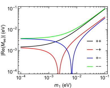
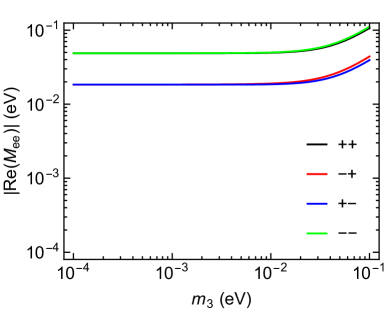
Figure 5: The possible values of $|{\rm Re}(M_{ee})|$ against the lightest neutrino mass $m_{1}$ (or $m_{3}$) in the NH (or IH) case for various combinations of $\rho^{(0)}$ and $\sigma^{(0)}$. The signs $++,-+,+-$ and $++$ respectively stand for $[\rho^{(0)},\sigma^{(0)}]=[0,0],[\pi/2,0],[0,\pi/2]$ and $[\pi/2,\pi/2]$.

2.2 Analytical approximations

In this section, we give the analytical expressions of $\Delta\delta$ and $\Delta\theta$ to explain the numerical results. After a lengthy but straightforward calculation, one obtains the approximation results

$$\Delta\delta \simeq [2{\rm T}(\overline{m}_{1}+\overline{m}_{2})(\overline{m}_{1}-m_{3})(\overline{m}_{2}-m_{3})\bar{s}_{13}]^{-1}\{[2{\rm T}m_{12}(m_{22}-m_{3})(\overline{m}_{1}+\overline{m}_{2}-2m_{3}s^{2}_{13})$$

$$-4m^{2}_{12}(m_{11}+m_{3}+{\rm T}m_{12})s^{2}_{13}+4(\overline{m}_{1}-m_{3})(\overline{m}_{2}-m_{3})(m_{11}+m_{3})s^{2}_{13}]{\rm R}_{1}-[4m_{12}$$

$$\times(\overline{m}_{1}-m_{3})(\overline{m}_{2}-m_{3})-2{\rm T}(\overline{m}_{1}+\overline{m}_{2}-2m_{3}s^{2}_{13})(m_{11}+m_{3})(m_{22}-m_{3})-4{\rm T}\Omega$$

$$\times m^{2}_{12}m_{3}s^{2}_{13}]\bar{s}_{13}{\rm I}_{1}-[{\rm T}m_{12}(m_{22}+m_{3})(\overline{m}_{1}+\overline{m}_{2}-2m_{3}s^{2}_{13})-2{\rm T}m_{12}(\overline{m}_{1}-m_{3})$$

$$\times(\overline{m}_{2}-m_{3})s^{2}_{13}-2(m_{11}-m_{3})(m_{22}+m_{3})(m_{11}+m_{3}+{\rm T}m_{12})s^{2}_{13}]{\rm R}_{2}$$

$$+{\rm T}(m_{22}+m_{3})[m^{2}_{12}-(m_{22}-m_{3})(2m_{11}+m_{22}-m_{3})]\bar{s}_{13}{\rm I}_{2}\}\;,$$

$$\Delta\theta \simeq [2{\rm T}(\overline{m}_{1}+\overline{m}_{2})(\overline{m}_{1}-m_{3})(\overline{m}_{2}-m_{3})]^{-1}\{2{\rm T}(\overline{m}_{1}+\overline{m}_{2})[m^{2}_{12}-(m^{2}_{11}-m^{2}_{3})s^{2}_{13}]{\rm R}_{1}$$ (24)

$$+4m_{11}m_{12}[{\rm T}(\overline{m}_{1}+\overline{m}_{2})+2m_{12}s^{2}_{13}]\bar{s}_{13}{\rm I}_{1}-{\rm T}(\overline{m}_{1}+\overline{m}_{2})(m_{11}-m_{3})(m_{22}+m_{3}){\rm R}_{2}$$

$$-{\rm T}m_{12}[(\overline{m}_{1}+\overline{m}_{2})(2m_{11}+m_{22}-m_{3})-2m_{11}(m_{22}+m_{3})s^{2}_{13}]\bar{s}_{13}{\rm I}_{2}\}\;,$$

with ${\rm T}=\tan{2\theta_{12}}$ and $\Omega=(m_{11}+m_{3})/(m_{11}-m_{3})$.

For illustration, we discuss the possible values of $\Delta\delta$ and $\Delta\theta$ in several typical cases. (1) In the case of $m_{1}\ll m_{2}\simeq\sqrt{\Delta m^{2}_{21}}\ll m_{3}\simeq\sqrt{|\Delta m^{2}_{31}|}$, $\Delta\delta$ and $\Delta\theta$ approximate to

$$\Delta\delta \simeq \frac{m_{3}}{2\overline{m}_{2}\bar{s}_{13}}\left[\left(2rc_{12}s_{12}+\frac{4}{{\rm T}}s^{2}_{13}\right){\rm R}_{1}-\bar{s}_{13}{\rm I}_{2}+\left(rc_{12}s_{12}-\frac{2}{{\rm T}}s^{2}_{13}\right){\rm R}_{2}\right]-2s^{2}_{12}{\rm I}_{1}\;,$$

$$\Delta\theta \simeq s^{2}_{13}{\rm R}_{1}-2|r|c_{12}s^{3}_{12}\bar{s}_{13}{\rm I}_{1}+\frac{1}{2}{\rm R}_{2}-\frac{\overline{m}_{2}}{2m_{3}}c_{12}s_{12}\bar{s}_{13}{\rm I}_{2}\;,$$ (25)

where $r=\Delta m^{2}_{21}/\Delta m^{2}_{31}$ has a value of $\pm 0.03$ for NH or IH. One can see that $\Delta\delta$ is susceptible to the symmetry breaking with the relevant coefficients having magnitudes of $\mathcal{O}(1)$, while $\Delta\theta$ is only sensitive to ${\rm R}_{2}$. (2) For $m_{1}\simeq m_{2}\simeq\sqrt{|\Delta m^{2}_{31}|}\gg m_{3}$, in which case one has $m_{2}-m_{1}\simeq\Delta m^{2}_{21}/(2\sqrt{|\Delta m^{2}_{31}|})$, the results are strongly dependent on the combinations of $\rho^{(0)}$ and $\sigma^{(0)}$. If they take the same value, $\Delta\delta$ and $\Delta\theta$ are simplified to

$$\Delta\delta \simeq {\rm I}_{1}-\frac{3}{4}{\rm I}_{2}+\frac{1}{4{\rm T}\bar{s}_{13}}\left[\left(4s^{2}_{13}-2{\rm T}|r|c_{12}s_{12}\right){\rm R}_{1}+\left(2s^{2}_{13}+{\rm T}|r|c_{12}s_{12}\right){\rm R}_{2}\right]\;,$$

$$\Delta\theta \simeq -s^{2}_{13}{\rm R}_{1}-|r|c_{12}s_{12}\bar{s}_{13}\left({\rm I}_{1}-\frac{3}{4}{\rm I}_{2}\right)-\frac{1}{2}{\rm R}_{2}\;.$$ (26)

Obviously, $|c^{\delta}_{i1}|$ and $|c^{\delta}_{i2}|$ are close to 1 but $|c^{\delta}_{r1}|$ and $|c^{\delta}_{r2}|$ are suppressed to a high level. Among the coefficients for $\Delta\theta$, only $|c^{\theta}_{r2}|$ is sizable. When $\rho^{(0)}$ and $\sigma^{(0)}$ differ from each other, one will have

$$\Delta\delta \simeq \frac{1}{|r|}\left[-32c^{3}_{12}s^{3}_{12}\bar{s}_{13}{\rm R}_{1}+4\cos{2\theta_{12}}{\rm I}_{1}-4c_{12}s_{12}\bar{s}_{13}{\rm R}_{2}-4c^{2}_{12}s^{2}_{12}\cos{2\theta_{12}}{\rm I}_{2}\right]\;,$$

$$\Delta\theta \simeq -4c^{2}_{12}s^{2}_{12}{\rm R}_{1}-c_{12}s_{12}\cos{2\theta_{12}}\left[1-\frac{4}{|r|}\cos{2\theta_{12}}s^{2}_{13}\right]\bar{s}_{13}\left(4{\rm I}_{1}-{\rm I}_{2}\right)-\frac{1}{2}\cos^{2}{2\theta_{12}}{\rm R}_{2}\;.$$ (27)

Enhanced by the factor $1/|r|$, the coefficients for $\delta$ can easily obtain some magnitudes $\geq 10$. While $|c^{\theta}_{r1}|$ with a value about 1 turns out to be the greatest coefficient for $\Delta\theta$. (3) When it comes to $m_{1}\simeq m_{2}\simeq m_{3}\simeq m_{0}$, in which case $m_{2}-m_{1}\simeq\Delta m^{2}_{21}/(2m_{0})$ and $m_{3}-m_{1}\simeq\Delta m^{2}_{31}/(2m_{0})$, the coefficients may get remarkably magnified in some cases. For $[\rho^{(0)},\sigma^{(0)}]=[0,0]$, $\Delta\delta$ and $\Delta\theta$ are approximately given by

$$\Delta\delta \simeq \frac{1}{{\rm T}\bar{s}_{13}}\left[\left({\rm T}rc_{12}s_{12}+2s^{2}_{13}\right){\rm R}_{1}+\frac{2m^{2}_{0}}{\Delta m^{2}_{31}}\left({\rm T}rc_{12}s_{12}-2s^{2}_{13}\right){\rm R}_{2}\right]-\frac{2m^{2}_{0}}{\Delta m^{2}_{31}}\left(2{\rm I}_{1}-{\rm I}_{2}\right)\;,$$

$$\Delta\theta \simeq \frac{2m^{2}_{0}}{\Delta m^{2}_{31}}\left[2s^{2}_{13}{\rm R}_{1}-rc_{12}s_{12}\bar{s}_{13}\left(2{\rm I}_{1}-{\rm I}_{2}\right)+{\rm R}_{2}\right]\;.$$ (28)

At $m_{0}\simeq 0.1$ eV, $|c^{\delta}_{i1}|$ and $|c^{\delta}_{i2}|$ are around 10 while $|c^{\delta}_{r1}|$ and $|c^{\delta}_{r2}|$ are only of $\mathcal{O}(0.1)$. $|c^{\theta}_{r2}|$ (with a value close to 10) is still the biggest coefficient for $\Delta\theta$. In the case of $[\rho^{(0)},\sigma^{(0)}]=[\pi/2,0]$, $\Delta\delta$ and $\Delta\theta$ appear as

$$\Delta\delta \simeq \frac{2m^{2}_{0}}{\Delta m^{2}_{21}}\left\{\left[\frac{4}{\rm T}s^{2}_{12}-2c_{12}s_{12}(1+2s^{2}_{12})\right]\bar{s}_{13}{\rm R}_{1}+2\cos{2\theta_{12}}{\rm I}_{1}-2c_{12}s_{12}\bar{s}_{13}{\rm R}_{2}-c^{2}_{12}{\rm I}_{2}\right\}\;,$$

$$\Delta\theta \simeq \frac{2m^{2}_{0}}{\Delta m^{2}_{31}}\left[2c^{2}_{12}s^{2}_{12}{\rm R}_{1}-\frac{4m^{2}_{0}}{\Delta m^{2}_{21}}c_{12}s_{12}\cos{2\theta_{12}}\bar{s}^{3}_{13}\left(2\cos{2\theta_{12}}{\rm I}_{1}-c^{2}_{12}{\rm I}_{2}\right)+c^{4}_{12}{\rm R}_{2}\right]\;.$$ (29)

When $[\rho^{(0)},\sigma^{(0)}]=[0,\pi/2]$, the results become

$$\Delta\delta \simeq \frac{2m^{2}_{0}}{\Delta m^{2}_{21}}\left\{-\left[\frac{4}{\rm T}c^{2}_{12}+2c_{12}s_{12}(1+2c^{2}_{12})\right]\bar{s}_{13}{\rm R}_{1}+2\cos{2\theta_{12}}{\rm I}_{1}-2c_{12}s_{12}\bar{s}_{13}{\rm R}_{2}+s^{2}_{12}{\rm I}_{2}\right\}\;,$$

$$\Delta\theta \simeq \frac{2m^{2}_{0}}{\Delta m^{2}_{31}}\left[2c^{2}_{12}s^{2}_{12}{\rm R}_{1}-\frac{4m^{2}_{0}}{\Delta m^{2}_{21}}c_{12}s_{12}\cos{2\theta_{12}}\bar{s}^{3}_{13}\left(2\cos{2\theta_{12}}{\rm I}_{1}+s^{2}_{12}{\rm I}_{2}\right)+s^{4}_{12}{\rm R}_{2}\right]\;.$$ (30)

For these two cases, the coefficients for $\Delta\delta$ may easily obtain a magnitude around 100 owing to the enhancement factor $m^{2}_{0}/\Delta m^{2}_{21}$, while those for $\Delta\theta$ just have some magnitudes of $\mathcal{O}(1)$ as the factor $m^{2}_{0}/\Delta m^{2}_{31}$ is not so significant. Finally, $[\rho^{(0)},\sigma^{(0)}]=[\pi/2,\pi/2]$ will lead us to

$$\Delta\delta \simeq -\frac{\Delta m^{2}_{31}}{4m^{2}_{0}\bar{s}_{13}}\left[\left(rc_{12}s_{12}+\frac{2}{{\rm T}}s^{2}_{13}\right){\rm R}_{1}+\bar{s}_{13}\left({\rm I}_{1}-{\rm I}_{2}\right)\right]\;,$$

$$\Delta\theta \simeq \frac{\Delta m^{2}_{31}}{8m^{2}_{0}}\left[2s^{2}_{13}{\rm R}_{1}-2rc_{12}s_{12}\bar{s}_{13}\left({\rm I}_{1}-{\rm I}_{2}\right)+{\rm R}_{2}\right]\;.$$ (31)

It is easy to see that all the coefficients are vanishingly small in this case. One will find that all the above analytical results agree well with the corresponding numerical results.

2.3 RG induced symmetry breaking

This section is devoted to the RG-induced breaking of $\mu$-$\tau$ reflection symmetry. A flavor symmetry [6] together with the associated new fields is usually introduced at an energy scale $\Lambda_{\rm FS}$ much higher than the electroweak (EW) one $\Lambda_{\rm EW}$. In this case one must consider the RG running effect when confronting the flavor-symmetry model with the low-energy data [19]. During the RG evolution process the significant difference between $m_{\mu}$ and $m_{\tau}$ can serve as a unique source for the breaking of $\mu$-$\tau$ reflection symmetry. As a result, the general symmetry breaking studied in the above finds an interesting application in such a specific situation [20, 21]. The energy dependence of neutrino mass matrix is described by its RG equation, which at the one-loop level appears as [22]

$$16\pi^{2}\frac{{\rm d}M_{\nu}}{{\rm d}t}=C\left(Y^{\dagger}_{l}Y_{l}\right)^{T}M_{\nu}+CM_{\nu}\left(Y^{\dagger}_{l}Y_{l}\right)+\alpha M_{\nu}\;.$$ (32)

Here $t$ is defined as $\ln(\mu/\mu_{0})$ with $\mu$ denoting the renormalization scale, whereas $C$ and $\alpha$ read

$$C=-\frac{3}{2}\;,\hskip 28.45274pt\alpha\simeq-3g^{2}_{2}+6y^{2}_{t}+\lambda\;,\hskip 28.45274pt{\rm in\ the\ SM}\;;$$

$$C=1\;,\hskip 28.45274pt\alpha\simeq-\frac{6}{5}g^{2}_{1}-6g^{2}_{2}+6y^{2}_{t}\;,\hskip 28.45274pt{\rm in\ the\ MSSM}\;.$$ (33)

In Eq. (32) the $\alpha$-term is flavor universal and therefore just contributes an overall rescaling factor (which will be referred to as $I_{\alpha}$), while the other two terms may modify the structure of $M_{\nu}$. In the basis under study, the Yukawa coupling matrix of three charged leptons is given by $Y_{l}={\rm Diag}(y_{e},y_{\mu},y_{\tau})$. In light of $y_{e}\ll y_{\mu}\ll y_{\tau}$, it is reasonable to neglect the contributions of $y_{e}$ and $y_{\mu}$. Integration of the RG equation enables us to connect the neutrino mass matrix $M_{\nu}(\Lambda_{\rm FS})$ at $\Lambda_{\rm FS}$ with the corresponding one at $\Lambda_{\rm EW}$ in a manner as [23]

$$M_{\nu}(\Lambda_{\rm EW})=I_{\alpha}I^{\dagger}_{\tau}M_{\nu}(\Lambda_{\rm FS})I^{*}_{\tau}\;,$$ (34)

where $I_{\tau}\simeq{\rm Diag}\{1,1,1-\Delta_{\tau}\}$ and

$$I_{\alpha}={\rm exp}\left(\frac{1}{16\pi^{2}}\int^{\ln\Lambda_{\rm EW}}_{\ln\Lambda_{\rm FS}}\alpha{\rm d}t\right),\hskip 28.45274pt\Delta_{\tau}=\frac{C}{16\pi^{2}}\int^{\ln\Lambda_{\rm FS}}_{\ln\Lambda_{\rm EW}}y^{2}_{\tau}{\rm d}t\;.$$ (35)

In the SM case, the RG running effect is negligible due to the smallness of $y_{\tau}\simeq 0.01$ (which renders $\Delta_{\tau}\simeq\mathcal{O}(10^{-5})$ ). By contrast, $y^{2}_{\tau}=(1+\tan^{2}{\beta})m^{2}_{\tau}/v^{2}$ can be enhanced by a large $\tan{\beta}$ in the MSSM case. Given $\Lambda_{\rm FS}\simeq 10^{13}$ GeV, for example, the value of $\Delta_{\tau}$ depends on $\tan{\beta}$ in a way as

$$\Delta_{\tau}\simeq 0.042\left(\displaystyle\frac{\tan{\beta}}{50}\right)^{2}\;.$$ (36)

With the help of Eq. (34), one will get the RG-corrected neutrino mass matrix at $\Lambda_{\rm EW}$

$$M_{\nu}(\Lambda_{\rm EW})\simeq I_{\alpha}\left[M_{\nu}(\Lambda_{\rm FS})-\Delta_{\tau}\left(\begin{matrix}0&0&M_{e\tau}\cr 0&0&M_{\mu\tau}\cr M_{e\tau}&M_{\mu\tau}&2M_{\tau\tau}\cr\end{matrix}\right)\right]\;,$$ (37)

from a neutrino mass matrix respecting the $\mu$-$\tau$ reflection symmetry at $\Lambda_{\rm FS}$. By means of the above-mentioned treatment, one may arrange $M_{\nu}(\Lambda_{\rm EW})$ in a form as given by Eq. (10) with $\epsilon_{2}=2\epsilon_{1}=\Delta_{\tau}$ and $\epsilon_{3,4}=0$, implying that $\Delta_{\tau}$ is the only quantity for measuring the symmetry-breaking strength. The relations between the mixing-parameter deviations and $\Delta_{\tau}$ can therefore be obtained by simply taking ${\rm R_{2}}=2{\rm R_{1}}=\Delta_{\tau}$ and ${\rm I_{1,2}}=0$ in Eq. (17). By solving these equations numerically, in Fig. 5 we display $c^{\theta}_{\tau}=\Delta\theta/\Delta_{\tau}$, $c^{\delta}_{\tau}=\Delta\delta/\Delta_{\tau}$, $c^{\rho}_{\tau}=\Delta\rho/\Delta_{\tau}$ and $c^{\sigma}_{\tau}=\Delta\rho/\Delta_{\tau}$ against the lightest neutrino mass $m_{1}$ ($m_{3}$) in the NH (IH) case for various combinations of $\rho^{(0)}$ and $\sigma^{(0)}$ with $\delta^{(0)}=-\pi/2$. In addition, some representative values of them at $m_{1}(m_{3})=0.001,0.01$ and 0.1 eV for the NH (IH) case in various situations are presented in Table 5. Since the relations $c^{\eta}_{\tau}=c^{\eta}_{r1}/2+c^{\eta}_{r2}$ (for $\eta=\theta,\delta,\rho$ and $\sigma$) hold, the coefficients associated with $\Delta_{\tau}$ closely resemble those associated with $r_{1,2}$ in a few aspects: (1) Their magnitudes tend to grow with the absolute neutrino mass scale (except in the case of $[\rho^{(0)},\sigma^{(0)}]=[\pi/2,\pi/2]$). (2) $|c^{\theta}_{\tau}|$ generally takes a value of $\mathcal{O}(1)$ in most cases, while $|c^{\delta}_{\tau}|$, $|c^{\rho}_{\tau}|$ and $|c^{\sigma}_{\tau}|$ may easily reach $\mathcal{O}(10)$ in the case of IH combined with $\rho^{(0)}\neq\sigma^{(0)}$. (3) $|c^{\delta}_{\tau}|$ and $|c^{\rho}_{\tau}|$ are comparable to each other in magnitude, while $|c^{\sigma}_{\tau}|$ is somewhat smaller. (4) $c^{\theta}_{\tau}$ is always positive (negative) in the NH (IH) case. With the help of these results, one can learn how much $\Delta\theta$ and $\Delta\delta$ are allowed by $\Delta_{\tau}\leq 0.04$ (for $\tan{\beta}\leq 50$): (1) In the case of $m_{1}\ll m_{2}\ll m_{3}$ or $m_{3}\ll m_{1}\simeq m_{2}$, $|\Delta\theta|$ is no greater than 0.02. When the neutrino masses are quasi-degenerate (except in the case of $[\rho^{(0)},\sigma^{(0)}]=[\pi/2,\pi/2]$), $\Delta_{\tau}\simeq 0.02$ (corresponding to $\tan{\beta}\simeq 35$) can lead to $|\Delta\theta|\simeq 0.1$. (2) $|\Delta\delta|$ is also no greater than 0.02 for $m_{1}\ll m_{2}\ll m_{3}$. When $m_{3}\ll m_{1}\simeq m_{2}$ is concerned, $|\Delta\delta|$ may reach 0.1 from $\Delta_{\tau}\simeq 0.005$ (or will be negligibly small) for $\rho^{(0)}\neq\sigma^{(0)}$ (or $\rho^{(0)}=\sigma^{(0)}$). In the case of $m_{1}\simeq m_{2}\simeq m_{3}$ combined with $\rho^{(0)}\neq\sigma^{(0)}$, even $\Delta_{\tau}\simeq 0.001$ can give rise to sizable $\Delta\delta$.

On the other hand, the analytical expressions for $c^{\theta}_{\tau}$, $c^{\delta}_{\tau}$ and $c^{\rho}_{\tau}$ are found to be

$$c^{\theta}_{\tau} \simeq [2(\overline{m}_{1}-m_{3})(\overline{m}_{2}-m_{3})]^{-1}[m^{2}_{12}-(m_{11}-m_{3})(m_{22}+m_{3})]\;,$$

$$c^{\delta}_{\tau} \simeq -\left[{\rm T}(\overline{m}_{1}+\overline{m}_{2})(\overline{m}_{1}-m_{3})(\overline{m}_{2}-m_{3})\overline{s}_{13}\right]^{-1}[{\rm T}m_{12}m_{3}(\overline{m}_{1}+\overline{m}_{2}-2m_{3}s^{2}_{13})$$

$$-2(m_{11}+{\rm T}m_{12}+m_{3})(\overline{m}_{1}\overline{m}_{2}-m_{22}m_{3})s^{2}_{13}]\;,$$

$$c^{\rho}_{\tau} \simeq -[2\overline{m}_{1}m_{3}(\overline{m}_{1}+\overline{m}_{2})(\overline{m}_{1}-m_{3})(\overline{m}_{2}-m_{3})\bar{s}_{13}t_{12}]^{-1}\{{\rm T}m_{12}m^{2}_{3}(\overline{m}_{1}+\overline{m}_{2})(m_{11}$$ (38)

$$-m_{3}s^{2}_{13}+2m_{22}t^{2}_{12}s^{2}_{13})-m_{11}[{\rm T}m_{12}m_{3}(\overline{m}_{1}+\overline{m}_{2}-2m_{3}s^{2}_{13})-2(m_{11}+{\rm T}m_{12}$$

$$+m_{3})(\overline{m}_{1}\overline{m}_{2}-m_{22}m_{3})s^{2}_{13}][m_{3}+m_{11}\Omega s^{2}_{13}-m_{22}t^{2}_{12}s^{2}_{13}]\}\;,$$

with $t_{12}=\tan{\theta_{12}}$, while $c^{\sigma}_{\tau}$ can be obtained from $\overline{m}_{1}c^{\rho}_{\tau}/\overline{m}_{2}$ by making the replacement $t_{12}\to-1/t_{12}$. These results can help us understand the numerical results: (1) For $m_{1}\ll m_{2}\ll m_{3}$, Eq. (38) is simplified to

$$c^{\theta}_{\tau}\simeq\frac{1}{2}\;,\hskip 28.45274ptc^{\delta}_{\tau}\simeq\frac{\overline{m}_{2}c_{12}s_{12}}{m_{3}\bar{s}_{13}}\;,\hskip 28.45274ptc^{\rho}_{\tau}\simeq\frac{c_{12}\bar{s}_{13}}{s_{12}}\;.$$ (39)

(2) In the case of $m_{1}\simeq m_{2}\gg m_{3}$, one will have

$$c^{\delta}_{\tau}\simeq\frac{1}{\rm T}\bar{s}_{13}\;,\hskip 28.45274ptc^{\rho}_{\tau}\simeq-\frac{[m_{3}+\overline{m}_{1}(1-t^{2}_{12})s^{2}_{13}]\bar{s}_{13}}{2m_{3}t_{12}}\;,$$ (40)

for $\rho^{(0)}=\sigma^{(0)}$, or

$$c^{\delta}_{\tau}\simeq-\frac{8}{|r|}c_{12}s_{12}\bar{s}_{13}\;,\hskip 28.45274ptc^{\rho}_{\tau}\simeq\frac{8[m_{3}+\overline{m}_{1}(c^{2}_{12}-s^{2}_{12})(1+t^{2}_{12})s^{2}_{13}]c^{3}_{12}s_{12}\bar{s}_{13}}{m_{3}|r|}\;,$$ (41)

for $\rho^{(0)}\neq\sigma^{(0)}$ together with $c^{\theta}_{\tau}\simeq-1/2$. (3) When the case of $m_{1}\simeq m_{2}\simeq m_{3}\simeq m_{0}$ is considered, the coefficients approximate to

$$c^{\theta}_{\tau}\simeq\frac{2m^{2}_{0}}{\Delta m^{2}_{31}}\;,\hskip 42.67912ptc^{\delta}_{\tau}\simeq\frac{2m^{2}_{0}[{\rm T}rc_{12}s_{12}-2s^{2}_{13}]}{{\rm T}\Delta m^{2}_{31}\overline{s}_{13}}\;,\hskip 59.75095ptc^{\rho}_{\tau}\simeq\frac{{\rm T}m^{2}_{0}rc^{2}_{12}}{\Delta m^{2}_{31}\bar{s}_{13}}\;;$$

$$c^{\theta}_{\tau}\simeq\frac{2m^{2}_{0}c^{2}_{12}}{\Delta m^{2}_{31}}\;,\hskip 37.55785ptc^{\delta}_{\tau}\simeq\frac{2m^{2}_{0}(r-4s^{2}_{13})c_{12}s_{12}}{\Delta m^{2}_{21}\bar{s}_{13}}\;,\hskip 65.44142ptc^{\rho}_{\tau}\simeq\frac{8m^{2}_{0}c^{3}_{12}s_{12}\bar{s}_{13}}{\Delta m^{2}_{21}}\;;$$

$$c^{\theta}_{\tau}\simeq\frac{2m^{2}_{0}s^{2}_{12}}{\Delta m^{2}_{31}}\;,\hskip 36.98866ptc^{\delta}_{\tau}\simeq-\frac{2m^{2}_{0}(r+4s^{2}_{13})c_{12}s_{12}}{\Delta m^{2}_{21}\bar{s}_{13}}\;,\hskip 56.9055ptc^{\rho}_{\tau}\simeq\frac{8m^{2}_{0}c^{3}_{12}s_{12}\bar{s}_{13}}{\Delta m^{2}_{21}}\;;$$

$$c^{\theta}_{\tau}\simeq\frac{\Delta m^{2}_{31}}{8m^{2}_{0}}\;,\hskip 42.67912ptc^{\delta}_{\tau}\simeq-\frac{{\rm T}\Delta m^{2}_{21}c_{12}s_{12}+2\Delta m^{2}_{31}s^{2}_{13}}{8{\rm T}m^{2}_{0}\overline{s}_{13}}\;,\hskip 28.45274ptc^{\rho}_{\tau}\simeq\frac{\Delta m^{2}_{31}\bar{s}_{13}}{8m^{2}_{0}t_{12}}\;,$$ (42)

for $[\rho^{(0)},\sigma^{(0)}]=[0,0]$, $[\pi/2,0]$, $[0,\pi/2]$ and $[\pi/2,\pi/2]$. One can see that these approximation results agree well with the corresponding numerical results.

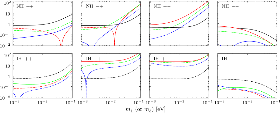
Figure 6: The coefficients associated with $\Delta_{\tau}$ ($c^{\theta}_{\tau}$ in black, $c^{\delta}_{\tau}$ in red, $c^{\rho}_{\tau}$ in green and $c^{\sigma}_{\tau}$ in blue) against the lightest neutrino mass $m_{1}$ (or $m_{3}$) in the NH (or IH) case for various combinations of $\rho^{(0)}$ and $\sigma^{(0)}$ with $\delta^{(0)}=-\pi/2$. The signs $++,-+,+-$ and $++$ respectively stand for $[\rho^{(0)},\sigma^{(0)}]=[0,0],[\pi/2,0],[0,\pi/2]$ and $[\pi/2,\pi/2]$.

		0.001 eV	0.01 eV	0.1 eV
$[0,0]$	$c^{\theta}_{\tau}$	0.65 [$-$0.55]	0.81 [$-$0.79]	6.63 [$-$15.6]
$[\pi/2,0]$		0.64 [$-$0.56]	0.69 [$-$0.67]	6.75 [$-$8.52]
$[0,\pi/2]$		0.40 [$-$0.54]	0.43 [$-$0.52]	3.44 [$-$4.91]
$[\pi/2,\pi/2]$		0.39 [$-$0.50]	0.31 [$-$0.35]	0.03 [$-$0.03]
$[0,0]$	$c^{\delta}_{\tau}$	$-$0.36 [$-$0.07]	$-$0.19 [$-$0.11]	0.46 [$-$2.39]
$[\pi/2,0]$		$-$0.40 [22.4]	$-$0.28 [24.6]	56.1 [180]
$[0,\pi/2]$		0.76 [22.2]	2.56 [21.9]	125 [89.9]
$[\pi/2,\pi/2]$		0.56 [$-$0.06]	0.19 [$-$0.04]	0.01 [-0.00]
$[0,0]$	$c^{\rho}_{\tau}$	$-$0.22 [0.20]	$-$0.19 [0.19]	$-$1.49 [3.56]
$[\pi/2,0]$		$-$0.27 [$-$6.02]	$-$0.92 [$-$15.2]	$-$58.9 [$-$98.3]
$[0,\pi/2]$		$-$0.24 [$-$25.0]	$-$0.94 [$-$17.1]	$-$65.3 [$-$93.9]
$[\pi/2,\pi/2]$		$-$0.19 [0.04]	$-$0.09 [0.07]	$-$0.01 [0.01]
$[0,0]$	$c^{\sigma}_{\tau}$	0.04 [0.02]	0.08 [$-$0.07]	0.65 [$-$1.50]
$[\pi/2,0]$		0.02 [2.47]	$-$0.25 [$-$6.34]	$-$24.1 [$-$45.2]
$[0,\pi/2]$		$-$0.03 [$-$16.5]	$-$0.35 [$-$8.26]	$-$29.2 [$-$42.9]
$[\pi/2,\pi/2]$		$-$0.01 [$-$0.12]	0.02 [$-$0.04]	0.00 [$-$0.00]

Table 5: Some representative values of the coefficients associated with $\Delta_{\tau}$ ($c^{\theta}_{\tau}$, $c^{\delta}_{\tau}$, $c^{\rho}_{\tau}$ and $c^{\sigma}_{\tau}$ successively) at $m_{1}(m_{3})=0.001,0.01$ and 0.1 eV in the NH (IH) case for various combinations of $\rho^{(0)}$ and $\sigma^{(0)}$ with $\delta^{(0)}=-\pi/2$.

3 Summary

To summarize, the $\mu$-$\tau$ reflection symmetry deserves particular attention as it leads to the interesting results $\theta_{23}=\pi/4$ and $\delta=\pm\pi/2$ (which are close to the current experimental data) as well as trivial Majorana phases. Nevertheless, it is reasonable for us to consider the breaking of such a symmetry either from the theoretical considerations (e.g., the RG running effect may provide a source for the symmetry breaking) or on the basis of experimental results (e.g., the newly-reported NOvA result disfavors the maximal mixing scenario at a 2.6$\sigma$ level). Consequently, we have performed a systematic study for the possible symmetry-breaking patterns and their implications for the mixing parameters.

We first define some parameters measuring the symmetry-breaking strengths and then derive an equation set relating them with the deviations of mixing parameters from the special values taken in the symmetry context. By solving these equations in both a numerical and analytical way, the sensitive strengths of mixing-parameter deviations to the symmetry-breaking parameters for various neutrino mass schemes and the Majorana-phase combinations are investigated in some detail. It turns out that $\Delta\theta$ is most sensitive to ${\rm R}_{2}$ while $\Delta\delta$, $\Delta\rho$ and $\Delta\sigma$ to all the symmetry-breaking parameters. The coefficients for for $\Delta\delta$, $\Delta\rho$ and $\Delta\sigma$ are generally much greater than those $\Delta\theta$ in magnitude. Furthermore, the coefficients tend to be magnified when the absolute neutrino mass scale increases (in particular for the case of $m_{1}\simeq m_{2}\simeq m_{3}$) and $\rho^{(0)}\neq\sigma^{(0)}$. With these general results as guide, one may easily find an appropriate specific way to break the $\mu$-$\tau$ reflection symmetry so as to generate the required mixing-parameter deviations when necessary. Finally, as a unique illustration, the general treatment is applied to the specific symmetry breaking induced by the RG running effect.

Acknowledgments    I would like to thank Professor Zhi-zhong Xing for fruitful collaboration on the $\mu$-$\tau$ flavor symmetry. This work is supported in part by the National Natural Science Foundation of China under grant No. 11605081.

References

- [1] K. A. Olive et al. (Particle Data Group), Chin. Phys. C 40, 100001 (2016).
- [2] F. Capozzi, E. Lisi, A. Marrone, D. Montanino and A. Palazzo, Phys. Rev. D 89, 093018 (2014).
- [3] P. A. R. Ade et al. (Planck Collaboration), arXiv:1502.01589.
- [4] P. Adamson et al. (NOvA Collaboration), arXiv:1701.05891.
- [5] I. Esteban, M. C. Gonzalez-Garcia, M. Maltoni, I. Martinez-Soler and T. Schwetz, JHEP 01, 087 (2017).
- [6] For some reviews, see G. Altarelli and F. Feruglio, Rev. Mod. Phys. 82, 2701 (2010); S. F. King and C. Luhn, Rept. Prog. Phys. 76, 056201 (2013).
- [7] T. Fukuyama and H. Nishiura, arXiv:hep-ph/9702253; E. Ma and M. Raidal, Phys. Rev. Lett. 87, 011802 (2001); C. S. Lam, Phys. Lett. B 507, 214 (2001); K. R. S. Balaji, W. Grimus and T. Schwetz, Phys. Lett. B 508, 301 (2001).
- [8] For a recent review with extensive references, see Z. Z. Xing and Z. H. Zhao, Rept. Prog. Phys. 79, 076201 (2016).
- [9] M. Apollonio et al. (CHOOZ Collaboration), Phys. Lett. B 420, 397 (1998).
- [10] F. P. An et al. (Daya Bay Collaboration), Phys. Rev. Lett. 108, 171803 (2012).
- [11] S. Gupta, A. S. Joshipura and K. M. Patel, JHEP 1309, 035 (2013).
- [12] P. F. Harrison and W. G. Scott, Phys. Lett. B 547, 219 (2002).
- [13] F. Feruglio, C. Hagedorn and R. Ziegler, JHEP 1307, 027 (2013); M. Holthausen, M. Lindner and M. A. Schmidt, JHEP 1304, 122 (2013).
- [14] W. Grimus and L. Lavoura, Phys. Lett. B 579, 113 (2004).
- [15] P. M. Ferreira, W. Grimus, L. Lavoura and P. O. Ludl, JHEP 09, 128 (2012); W. Grimus and L. Lavoura, Fortsch. Phys. 61, 535 (2013); R. N. Mohapatra and C. C. Nishi, Phys. Rev. D 86, 073007 (2012); JHEP 1508, 092 (2015); E. Ma, A. Natale and O. Popov, Phys. Lett. B 746, 114 (2015); E. Ma, Phys. Rev. D 92, 051301 (2015); Phys. Lett. B 752, 198 (2016); A. S. Joshipura and K. M. Patel, Phys. Lett. B 749, 159 (2015); H. J. He, W. Rodejohann and X. J. Xu, Phys. Lett. B 751, 586 (2015); C. C. Nishi, Phys. Rev. D 93, 093009 (2016); P. M. Ferreira, W. Grimus, D. Jurciukonis and L. Lavoura, JHEP 07, 010 (2016); A. S. Joshipura and N. Nath, Phys. Rev. D 94, 036008 (2016); C. C. Li, J. N. Lu and G. J. Ding, Nucl. Phys. B 913, 110 (2016); C. C. Nishi and B. L. S nchez-Vega, JHEP 01, 068 (2017); W. Rodejohann and X. J. Xu, arXiv:1705.02027; Z. Z. Xing and J. Y. Zhu, arXiv:1707.03676; Z. C. Liu, C. X. Yue and Z. H. Zhao, arXiv:1707.05535.
- [16] W. Grimus, A. S. Joshipura, S. Kaneko, L. Lavoura, H. Sawanaka and M. Tanimoto, Nucl. Phys. B 713, 151 (2005).
- [17] For a review with extensive references, see: W. Rodejohann, Int. J. Mod. Phys. E 20, 1833 (2011); S. M. Bilenky and C. Giunti, Int. J. Mod. Phys. A 30, 0001 (2015); S. Dell’Oro, S. Marcocci, M. Viel and F. Vissani, Adv. High Energy Phys. 2016, 2162659 (2016); J. D. Vergados, H. Ejiri and F. Simkovic, Int. J. Mod. Phys. E 25, 1630007 (2016).
- [18] See also R. N. Mohapatra and C. C. Nishi, JHEP 1508, 092 (2015).
- [19] T. Ohlsson and S. Zhou, Nature Commun. 5, 5153 (2014).
- [20] Y. L. Zhou, arXiv:1409.8600.
- [21] See also Y. H. Ahn, S. K. Kang, C. S. Kim and T. P. Nguyen, arXiv:0811.1458; S. Luo and Z. Z. Xing, Phys. Rev. D 90, 073005 (2014); J. Zhang and S. Zhou, JHEP 1609, 167 (2016).
- [22] P. H. Chankowski and Z. Pluciennik, Phys. Lett. B 316, 312 (1993); K. S. Babu, C. N. Leung and J. Pantaleone, Phys. Lett. B 319, 191 (1993); S. Antusch, M. Drees, J. Kersten, M. Lindner and M. Ratz, Phys. Lett. B 519, 238 (2001); Phys. Lett. B 525, 130 (2002); S. Antusch, J. Kersten, M. Lindner and M. Ratz, Nucl. Phys. B 674, 401 (2003).
- [23] J. R. Ellis and S. Lola, Phys. Lett. B 458, 310 (1999); P. H. Chankowski, W. Krolikowski and S. Pokorski, Phys. Lett. B 473, 109 (2000).