Tracking Gaze and Visual Focus of Attention of People Involved in Social Interaction

Abstract

The visual focus of attention (VFOA) has been recognized as a prominent conversational cue. We are interested in estimating and tracking the VFOAs associated with multi-party social interactions. We note that in this type of situations the participants either look at each other or at an object of interest; therefore their eyes are not always visible. Consequently both gaze and VFOA estimation cannot be based on eye detection and tracking. We propose a method that exploits the correlation between eye gaze and head movements. Both VFOA and gaze are modeled as latent variables in a Bayesian switching state-space model. The proposed formulation leads to a tractable learning procedure and to an efficient algorithm that simultaneously tracks gaze and visual focus. The method is tested and benchmarked using two publicly available datasets that contain typical multi-party human-robot and human-human interactions.

I Introduction

In this paper we are interested in the computational analysis of social interactions. In addition to speech, people communicate via a large variety of non-verbal cues, e.g. prosody, hand gestures, body movements, head nodding, eye gaze, and facial expressions. For example, in a multi-party conversation, a common behavior consists in looking either at a person, e.g. the speaker, or at an object of current interest, e.g. a computer screen, a painting on a wall, or an object lying on a table. We are particularly interested in estimating the visual focus of attention (VFOA), or who is looking at whom or at what, which has been recognized as one of the most prominent social cues. It is used in multi-party dialog to establish face-to-face communication, to respect social etiquette, to attract someone’s attention, or to signify speech-turn taking, thus complementing speech communication.

The VFOA characterizes a perceiver/target pair. It may be defined either by the line from the perceiver’s face to the perceived target, or by the perceiver’s direction of sight or gaze direction (which is often referred to as eye gaze or simply gaze). Indeed, one may state that the VFOA of person $i$ is target $j$ if the perceiver’s gaze is aligned with the perceiver-to-target line. From a physiological point of view, eye gaze depends on both eyeball orientation and head orientation. Both the eye and the head are rigid bodies with three and six degrees of freedom respectively. The head position (three coordinates) and the head orientation (three angles) are jointly referred to as the head pose. With proper choices for the head- and eye-centered coordinate frames, one can assume that gaze is a combination of head pose and of eyeball orientation, and the VFOA depends on head pose, eyeball orientation, and target location.

In this paper we are interested into estimating and tracking jointly the VFOAs of a group of people that communicate with each other and with a robot, or multi-party HRI (human-robot interaction), which may well be viewed as a generalization of single-user HRI. From a methodological point of view the former is more complex than the latter. Indeed, in single-user HRI the person and the robot face each other and hence a camera mounted onto the robot head provides high-resolution frontal images of the user’s face such that head pose and eye orientation can both be easily and robustly estimated. In the case of multi-party HRI the eyes are barely detected since the participants often turn their faces away from the camera. Consequently, VFOA estimation methods based on eye detection and eye tracking are ineffective and one has to estimate the VFOA, indirectly, without explicit eye detection.

We propose a Bayesian switching dynamic model for the estimation and tracking gaze directions and VFOAs of several persons involved in social interaction. While it is assumed that head poses (location and orientation) and target locations can be directly detected from the data, the unknown gaze directions and VFOAs are treated as latent random variables. The proposed temporal graphical model, that incorporates gaze dynamics and VFOA transitions, yields (i) a tractable learning algorithm and (ii) an efficient gaze-and-VFOA tracking method. The proposed method may well be viewed as a computational model of [1, 2].

The method is evaluated using two publicly available datasets, Vernissage [3] and LAEO [4]. These datasets consist of several hours of video containing situated dialog between two persons and a robot (Vernissage) and human-human interactions (LAEO). We are particularly interested in finding participants that either gaze to each other, gaze to the robot, or gaze to an object. Vernissage is recorded with a motion capture system (a network of infrared cameras) and with a camera placed onto the robot head. LAEO is collected from TV shows.

The remainder of this paper is organized as follows. Section II provides an overview of related work in gaze, VFOA and head-pose estimation. Section III introduces the paper’s mathematical notations and definitions, states the problem formulation and describes the proposed model. Section IV presents in detail the model inference and Section  V derives the learning algorithm. Section VI provides implementation details and Section VII describes the experiments and reports the results.

II Related Work

As already mentioned, the VFOA is correlated with gaze. Several methods proceed in two steps, in which the gaze direction is estimated first, and then used to estimate VFOA. In scenarios that rely on precise estimation of gaze [5, 6] a head-mounted camera, like the one in [7], can be used to detect the iris with high accuracy. Head-mounted eye trackers provide extremely accurate gaze measurements and in some circumstances eye-tracking data can be used to estimate objects of interest in videos [8]. Nevertheless, they are invasive instruments and hence not appropriate for analyzing social interactions.

Gaze estimation is relevant for a number of scenarios, such as car driving [9] or interaction with smartphones [10]. In these situations, either the field of view is limited, hence the range of gaze directions is constrained (car driving), or active human participation ensures that the device yields frontal views of the user’s face, thus providing accurate eye measurements [7, 9, 11, 12]. In some scenarios the user is even asked to limit head movements [13], or to proceed through a calibration phase [12, 14]. Even if no specific constraints are imposed, single-user scenarios inherently facilitate the task of eye measurement [11]. At the best of our knowledge, there is no gaze estimation method that can deal with unconstrained scenarios, e.g. participants not facing the cameras, partially or totally occluded eyes, etc. In general, eye analysis is inaccurate when participants are faraway from the camera.

An alternative is to approximate gaze direction with head pose [15]. Unlike eye-based methods, head pose can be estimated from low-resolution images, i.e. distant cameras [16, 17, 18, 19, 20]. These methods estimate gaze only approximatively since eyeball orientation can differ from head orientation by $\pm 35\degree$ [21]. Gaze estimation from head orientation can benefit from the observation that gaze shifts are often achieved by synchronously moving the head and the eyes [22, 1, 2]. The correlation between head pose and gaze has also been exploited in [23]. More recently, [24] combined head and eye features to estimate the gaze direction using an RGB-D camera. The method still requires that both eyes are visible.

Several methods were proposed to infer VFOAs either from gaze directions [25], or from head poses [4, 26, 27, 28]. For example, in [4] it is proposed to build a gaze cone around the head orientation and targets lying inside this cone are used to estimate the VFOA. While this method was successfully applied to movies, its limitation resides in its vagueness: the VFOA information is limited to whether there are two people looking at each other or not.

An interesting application of VFOA estimation it the analysis of social behavior of participants engaged in meetings, e.g.  [23, 26, 29, 30]. Meetings are characterized by interactions between seated people that interact based on speech and on head movements. Some methods estimate the most likely VFOA associated with a head orientation [23, 29]. The drawback of these approaches is that they must be purposively trained for each particular meeting layout. The correlation between VFOA and head pose was also investigated in [26] where an HMM is proposed to infer VFOAs from head and body orientations. This work was extended to deal with more complex scenarios, such as participants interacting with a robot [27, 31]. An input-output HMM is proposed in [31] to enable to model the following contextual information: participants tend to look to the speaker, to the robot, or to an object which is referred to by the speaker or by the robot. The results of [31] show that this improves the performance of VFOA estimation. Nevertheless, this method requires additional information, such as speaker identification or speech recognition.

The problem of joint estimation of gaze and of VFOA was addressed in a human-robot cooperation task [28]. In such a scenario the user doesn’t necessarily face the camera and robot-mounted cameras have low-resolution, hence the estimation of gaze from direct analysis of eye regions is not feasible. [28] proposes to learn a regression between the space of head poses and the space of gaze directions and then to predict an unknown gaze from an observed head pose. The head pose itself is estimated by fitting a 3D elliptical cylinder to a detected face, while the associated gaze direction corresponds to the 3D line joining the head center to the target center. This implies that during the learning stage, the user is instructed to gaze at targets lying on a table in order to provide training data. The regression parameters thus estimated correspond to a discrete set of head-pose/gaze-direction pairs (one for each target); an erroneous gaze may be predicted when the latter is not in the range of gaze directions used for training.

A summary of the proposed Bayesian dynamic model and experiments with the Vernissage [3] motion capture dataset were presented in [32]. In this article we provide a detailed and comprehensive description and analysis of the proposed model, of the model inference, of the learning methodology, and of the associated algorithms. We show results with both motion capture and RGB data from Vernissage. Additionally, we show results with the LAEO dataset [4].

III Proposed Model

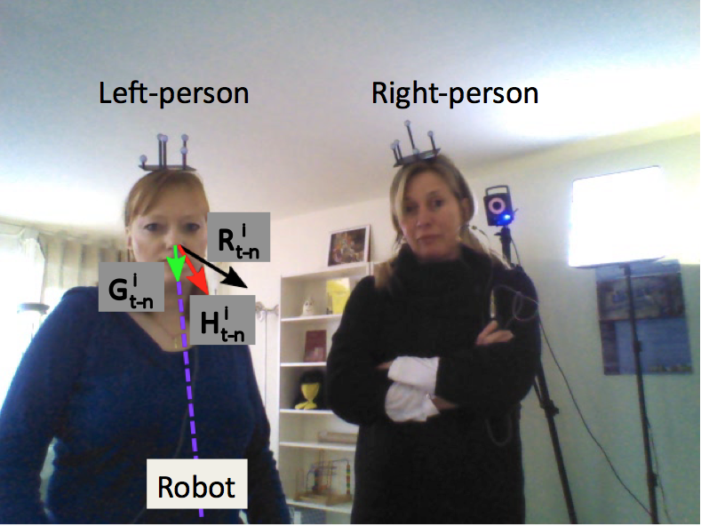
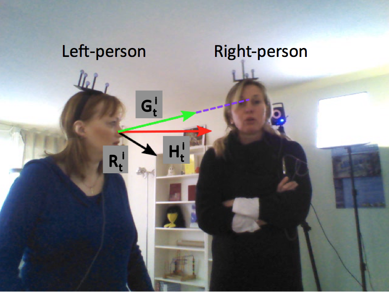
Figure 1: This figure illustrates the principle of our method and displays the observed and latent variables associated with a person (left-person indexed by $i$). The two images were grabbed with a camera mounted onto the head of a robot and they correspond to frames $t-n$ (left image) and $t$ (right image), respectively. The following variables are displayed: head orientation (red arrow), $\mathbf{H}_{t-n}^{i},\mathbf{H}_{t}^{i}$ (observed variables), as well as the latent variables estimated with the proposed method, namely gaze direction (green arrow), $\mathbf{G}_{t-n}^{i},\mathbf{G}_{t}^{i}$, VFOA, $\mathrm{V}_{t-n}^{i},\mathrm{V}_{t}^{i}$, and head reference orientation (black arrow), $\mathbf{R}_{t-n}^{i},\mathbf{R}_{t}^{i}$ (that coincides with upper-body orientation). In this example left-person gazes towards the robot at $t-n$, then turns her head to eventually gaze towards right-person at $t$, hence her VFOA switches from $\mathrm{V}_{t-n}^{i}=\textit{robot}$ to $\mathrm{V}_{t}^{i}=\textit{right-person}$.

The proposed mathematical model model is inspired from psychophysics [1, 2]. In unconstrained scenarios a person switches his/her gaze from one target to another target, possibly using both head and eye movements. Quick eye movements towards a desired object of interest are called saccades. Eye movements can also be caused by the vestibule-ocular reflex that compensates for head movements such that one can maintain his/her gaze in the direction of the target of interest. Therefore, in the general case, gazing to an object is achieved by a combination of eye and head movements.

In the case of small gaze shifts, e.g. reading or watching TV, eye movements are predominant. In the case of large gaze shifts, often needed in social scenarios, head movements are necessary since eyeball movements have limited range, namely $\pm$35° [21]. Therefore, the proposed model considers that gaze shifts are produced by head movements that occur simultaneously with eye movements.

III-A Problem Formulation

We consider a scenario composed of $N$ active targets and $M$ passive targets. An active target is likely to move and/or to have a leading role in an interaction. Active targets are persons and robots. Passive targets are objects, e.g. wall paintings. The set of all targets is indexed from $0$ to $N+M$, where the index $0$ designates “no target". Let $i$ be an active target (a person or a robot), $1\leq i\leq N$, and $j$ be a passive target (an object), $N+1\leq j\leq N+M$. A VFOA is a discrete random variable defined as follows: $\mathrm{V}_{t}^{i}=j$ means person (or robot) $i$ looks at target $j$ at time $t$. The VFOA of a person (or robot) $i$ that looks at none of the known targets is $\mathrm{V}_{t}^{i}=0$. The case $\mathrm{V}_{t}^{i}=i$ is excluded. The set of all VFOAs at time $t$ is denoted by $\mathbf{V}_{t}=\left(\mathrm{V}_{t}^{1},\ldots,\mathrm{V}_{t}^{N}\right)$.

Two continuous variables are now defined: head orientation and gaze direction. The head orientation of person $i$ at $t$ is denoted with $\mathbf{H}_{t}^{i}=[\phi_{H,t}^{i},\theta_{H,t}^{i}]^{\top}$, i.e. the pan and tilt angles of the head with respect to some fixed coordinate frame. The gaze direction of person $i$ is denoted with $\mathbf{G}_{t}^{i}$ and is also parameterized by pan and tilt with respect to the same coordinate frame, namely $\mathbf{G}_{t}^{i}=[\phi_{G,t}^{i},\theta_{G,t}^{i}]^{\top}$. Although eyeball orientation is neither needed nor used, it is worth noticing that it is the difference between $\mathbf{G}_{t}^{i}$ and $\mathbf{H}_{t}^{i}$. These variables are illustrated on Fig. 1.

Finally, to establish a link between VFOAs and gaze directions, the target locations must be defined as well. Let $\mathbf{X}_{t}^{i}=[x_{t}^{i},y_{t}^{i},z_{t}^{i}]^{\top}$ be the location of target $i$. In the case of a person, this location corresponds to the head center while in the case of a passive target, it corresponds to the target center. These locations are defined in the same coordinate frame as above. Also notice that the direction from the active target $i$ to target $j$ is defined by the unit vector $\mathbf{X}_{t}^{ij}=(\mathbf{X}_{t}^{j}-\mathbf{X}_{t}^{i})/\|\mathbf{X}_{t}^{j}-\mathbf{X}_{t}^{i}\|$ which can also be parameterized by two angles, $\mathbf{X}_{t}^{ij}=[\phi_{X,t}^{i,j},\theta_{X,t}^{i,j}]^{\top}$.

As already mentioned, target locations and head orientations are observed random variables, while VFOAs and gaze directions are latent random variables. The problem to be solved can now be formulated as a maximum a posteriori (MAP) problem:

$$\hat{\mathbf{V}}_{t},\hat{\mathbf{G}}_{t} =\operatorname*{argmax}_{\mathbf{V}_{t},\mathbf{G}_{t}}P(\mathbf{V}_{t},\mathbf{G}_{t}|\mathbf{H}_{1:t},\mathbf{X}_{1:t})$$ (1)

Since there is no deterministic relationship between head orientation and gaze direction, we propose to model it probabilistically. For this purpose, we introduce an additional latent random variable, namely the head reference orientation, $\mathbf{R}_{t}^{i}=[\phi_{R,t}^{i},\theta_{R,t}^{i}]^{\top}$, which we choose to coincide with the upper-body orientation. We use the following generative model, initially introduced in [26], linking gaze direction, head orientation, and head reference orientation:

$$P(\mathbf{H}_{t}^{i}|\mathbf{G}_{t}^{i},\mathbf{R}_{t}^{i};\boldsymbol{\alpha},\boldsymbol{\Sigma}_{\mathbf{H}}) =\mathcal{N}(\mathbf{H}_{t}^{i};\boldsymbol{\mu}_{\mathbf{H},t}^{i},\boldsymbol{\Sigma}_{\mathbf{H}}),$$ (2)

$$\textrm{with}\quad\boldsymbol{\mu}_{\mathbf{H},t}^{i} =\boldsymbol{\alpha}\mathbf{G}_{t}^{i}+(\mathbf{I}_{2}-\boldsymbol{\alpha})\mathbf{R}_{t}^{i},$$ (3)

where $\boldsymbol{\Sigma}_{\mathbf{H}}\in\mathbb{R}^{2\times 2}$ is a covariance matrix, $\mathbf{I}_{2}\in\mathbb{R}^{2\times 2}$ is the identity matrix and $\boldsymbol{\alpha}=\operatorname{Diag\,}(\alpha_{1},\alpha_{2})$ is a diagonal matrix of mixing coefficients, $0<\alpha_{1},\alpha_{2}<1$. Also it is assumed that the covariance matrix is the same for all the persons and over time. Therefore, head orientation is an observed random variable normally distributed around a convex combination between two latent variables: gaze direction and head reference orientation.

III-B Gaze Dynamics

The following model is proposed:

$$P(\mathbf{G}_{t}^{i}|\mathbf{G}_{t-1}^{i}\mathbf{\dot{G}}_{t-1}^{i},\mathrm{V}_{t}^{i}=j,\mathbf{X}_{t}) =\mathcal{N}(\mathbf{G}_{t}^{i};\boldsymbol{\mu}_{\mathbf{G},t}^{ij},\boldsymbol{\Gamma}_{\mathbf{G}}),$$ (4)

$$P(\mathbf{\dot{G}}_{t}^{i}|\mathbf{\dot{G}}_{t-1}^{i}) =\mathcal{N}(\mathbf{\dot{G}}_{t}^{i};\mathbf{\dot{G}}_{t-1}^{i},\boldsymbol{\Gamma}_{\mathbf{\dot{G}}}),$$ (5)

with:

$$\boldsymbol{\mu}_{\mathbf{G},t}^{ij}=\begin{cases}\mathbf{G}_{t-1}^{i}+\mathbf{\dot{G}}_{t-1}^{i}\>dt,&\mbox{if}\>j=0,\\ \boldsymbol{\beta}\mathbf{G}_{t-1}^{i}+(\mathbf{I}_{2}-\boldsymbol{\beta})\mathbf{X}_{t}^{ij}+\mathbf{\dot{G}}_{t-1}^{i}\>dt,&\mbox{if}\>j\neq 0,\end{cases}$$ (6)

where $\mathbf{\dot{G}}_{t}^{i}=d\mathbf{G}_{t}^{i}/dt$ is the gaze velocity, $\boldsymbol{\Gamma}_{\mathbf{G}},\boldsymbol{\Gamma}_{\mathbf{\dot{G}}}\in\mathbb{R}^{2\times 2}$ are covariance matrices, and $\boldsymbol{\beta}=\operatorname{Diag\,}(\beta_{1},\beta_{2})$ is a diagonal matrix of mixing coefficients, $0<\beta_{1},\beta_{2}<1$. Therefore, if a person looks at one of the targets, then his/her gaze dynamics depends on the person-to-target direction $\mathbf{X}_{t}^{ij}$ at a rate equal to $\boldsymbol{\beta}$, and if a person doesn’t look at one of the targets, then his/her gaze dynamics follows a random walk.

The head reference orientation dynamics can be defined in a similar way:

$$P(\mathbf{R}_{t}^{i}|\mathbf{R}_{t-1}^{i},\mathbf{\dot{R}}_{t-1}^{i}) =\mathcal{N}(\mathbf{R}_{t}^{i};\boldsymbol{\mu}_{\mathbf{R},t}^{i},\boldsymbol{\Gamma}_{\mathbf{R}}),$$ (7)

$$P(\mathbf{\dot{R}}_{t}^{i}|\mathbf{\dot{R}}_{t-1}^{i}) =\mathcal{N}(\mathbf{\dot{R}}_{t}^{i};\mathbf{\dot{R}}_{t-1}^{i},\boldsymbol{\Gamma}_{\mathbf{\dot{R}}}),$$ (8)

$$\textrm{with}\;\boldsymbol{\mu}_{\mathbf{R},t}^{i} =\mathbf{R}_{t-1}^{i}+\mathbf{\dot{R}}_{t-1}^{i}\>dt,$$

where $\mathbf{\dot{R}}_{t}^{i}=d\mathbf{R}_{t}^{i}/dt$ is the head reference orientation velocity and $\boldsymbol{\Gamma}_{\mathbf{R}},\boldsymbol{\Gamma}_{\mathbf{\dot{R}}}\in\mathbb{R}^{2\times 2}$ are covariance matrices. The dependencies between all the model variables are shown as a graphical representation in Figure 2.

Figure 2: Graphical representation showing the dependencies between the variables of the proposed Bayesian dynamic model. The discrete latent variables (visual focus of attention) are shown with squares while continuous variables are shown with circles: observed variables (head pose and target locations) are shown with shaded circles and latent variables (gaze and reference) are shown with white circles.

It is assumed that the gaze directions associated with different people are independent, given the VFOAs $\mathbf{V}_{1:t}$. The cross-dependency between different people is taken into account by the VFOA dynamics as detailed in section III-C below. Similarly, head orientations, and head reference orientations associated with different people are independent, given the VFOAs. By combining the above equations with this independency assumption, we obtain:

$$P(\mathbf{H}_{t}|\mathbf{G}_{t},\mathbf{R}_{t}) =\prod_{i}\mathcal{N}(\mathbf{H}_{t}^{i};\boldsymbol{\mu}_{\mathbf{H},t}^{i},\boldsymbol{\Sigma}_{\mathbf{H}})$$ (9)

$$P(\mathbf{G}_{t}|\mathbf{G}_{t-1},\mathbf{\dot{G}}_{t-1},\mathbf{V}_{t},\mathbf{X}_{t}) =\prod_{i,j}\mathcal{N}(\mathbf{G}_{t}^{i};\boldsymbol{\mu}_{\mathbf{G},t}^{ij},\boldsymbol{\Gamma}_{\mathbf{G}})^{\delta_{j}(\mathbf{V}_{t}^{i})}$$ (10)

$$P(\mathbf{R}_{t}|\mathbf{R}_{t-1},\mathbf{\dot{R}}_{t-1}) =\prod_{i}\mathcal{N}(\mathbf{R}_{t}^{i};\boldsymbol{\mu}_{\mathbf{R},t}^{i},\boldsymbol{\Gamma}_{\mathbf{R}})$$ (11)

where the dependencies between variables are embedded in the variable means, i.e. (3) and (6). The covariance matrices will be estimated via training. While gaze directions can vary a lot, we assume that head reference orientations are almost constant over time, which can be enforced by imposing that the total variance of gaze is much larger than the total variance of head reference orientation, namely:

$$\operatorname{Tr}(\boldsymbol{\Gamma}_{\mathbf{G}})\gg\operatorname{Tr}(\boldsymbol{\Gamma}_{\mathbf{R}}),$$ (12)

III-C VFOA Dynamics

Using a first-order Markov approximation, the VFOA transition probabilities can be written as:

$$P(\mathbf{V}_{t}|\mathbf{V}_{1:t-1})=P(\mathbf{V}_{t}|\mathbf{V}_{t-1}),$$ (13)

Notice that matrix $P(\mathbf{V}_{t}|\mathbf{V}_{t-1})$ is of size $(N+M)^{N}\times(N+M)^{N}$. Indeed, there are $N$ persons (active targets), and $N+M+1$ targets (one "no" target, N active targets and $M$ passive targets) and the case of a person that looks to him/herself is excluded. For example, if $N=2$ and $M=4$, matrix (13) has $(2+4)^{2\times 2}=1296$ entries. The estimation of this matrix would require, in principle, a large amount of training data, in particular in the presence of many symmetries. We show that, in practice, only 15 different transitions are possible. This can be seen on the following grounds.

We start by assuming conditional independence between the VFOAs at $t$:

$$P(\mathbf{V}_{t}|\mathbf{V}_{t-1}) =\prod_{i}P(\mathrm{V}_{t}^{i}|\mathbf{V}_{t-1}).$$ (14)

Let’s consider $V_{t}^{i}$, the VFOA of person $i$ at $t$, given $\mathbf{V}_{t-1}$, the VFOAs at $t-1$. One can distinguish two cases:

• $V_{t-1}^{i}=k$ where $k$ is either a passive target, $N<k\leq N+M$, or it is none of the targets, $k=0$; in this case $V_{t}^{i}$ depends only on $V_{t-1}^{i}$, and

• $V_{t-1}^{i}=k$, where $k\neq i$ is a person $1\leq k\leq N$; in this case $V_{t}^{i}$ depends on the both $V_{t-1}^{i}$ and $V_{t-1}^{k}$.

To summarize, we can write that:

$$P( \mathrm{V}_{t}^{i}=j|\mathbf{V}_{t-1})=$$

$$\begin{cases}P(\mathrm{V}_{t}^{i}=j|\mathrm{V}_{t-1}^{i}=k,\mathrm{V}_{t-1}^{k}=l)&\text{if}\;1\leq k\leq N,\\ P(\mathrm{V}_{t}^{i}=j|\mathrm{V}_{t-1}^{i}=k)&\text{otherwise}.\end{cases}$$ (15)

Based on this it is now possible to count the total number of possible VFOA transitions. With the same notations as in (III-C), we have the following possibilities:

• $k=0$ (no target): there are two possible transitions, $j=0$ and $j\neq 0$.

• $N<k\leq N+M$ (passive target): there are three possible transitions, $j=0$, $j=k$, and $j\neq k$.

• $1\leq k\leq N,l=0$ (active target $k$ looks at no target): there are three possible transitions, $j=0$, $j=k$, and $j\neq k$.

• $1\leq k\leq N,l=i$ (active target $k$ looks at person $i$): there are three possible transitions, $j=0$, $j=k$, and $j\neq k$.

• $1\leq k\leq N,l\neq 0,i$ (active target $k$ looks at active target $l$ different than $i$): there are four possible transitions, $j=0$, $j=k$, $j=l$ and $j\neq k,l$.

Therefore, there are 15 different possibilities for $P(\mathrm{V}_{t}^{i}=j|\mathbf{V}_{t-1})$, i.e. appendix A. Moreover, by assuming that the VFOA transitions don’t depend on $i$, we conclude that the transition matrix may have up to 15 different entries. Moreover, the number of possible transitions is even smaller if there is no passive target ($M=0$), or if the number of active targets is small, e.g. $N<3$. This considerably simplifies the task of estimating this matrix and makes the task of learning tractable.

IV Inference

We start by simplifying the notation, namely $\mathbf{L}_{t}=[\mathbf{G}_{t};\dot{\mathbf{G}}_{t};\mathbf{R}_{t};\dot{\mathbf{R}}_{t}]$ where $[\cdot;\cdot]$ denotes vertical concatenation. The emission probabilities (9) become:

$$P(\mathbf{H}_{t}|\mathbf{L}_{t}) =\prod_{i}\mathcal{N}(\mathbf{H}_{t}^{i};\boldsymbol{\mu}_{\mathbf{H},t}^{i},\boldsymbol{\Sigma}_{\mathbf{H}}),$$ (16)

$$\textrm{with}\quad\boldsymbol{\mu}_{\mathbf{H},t}^{i} =\mathbf{C}\mathbf{L}_{t}^{i},$$ (17)

where matrix $\mathbf{C}$ is obtained from the definition of $\mathbf{L}_{t}$ above and from (3):

$$\mathbf{C}=\begin{pmatrix}\alpha_{1}&0&0&0&1-\alpha_{1}&0&0&0\\ 0&\alpha_{2}&0&0&0&1-\alpha_{2}&0&0\end{pmatrix}.$$

The transition probabilities can be obtained by combining (10) and (11) with (5) and (8):

$$P(\mathbf{L}_{t}|\mathbf{V}_{t},\mathbf{L}_{t-1},\mathbf{X}_{t}) =\prod_{i}\prod_{j}\mathcal{N}(\mathbf{L}_{t}^{i};\boldsymbol{\mu}_{\mathbf{L},t}^{ij},\Gamma_{\mathbf{L}})^{\delta_{j}(\mathrm{V}_{t}^{i})},$$ (18)

$$\textrm{with}\quad\boldsymbol{\mu}_{\mathbf{L},t}^{ij} =\mathbf{A}_{t}^{ij}\mathbf{L}_{t-1}^{i}+\mathbf{b}_{t}^{ij}$$ (19)

$$\textrm{and}\quad\boldsymbol{\Gamma}_{\mathbf{L}} =\begin{pmatrix}\boldsymbol{\Gamma}_{\mathbf{G}}&&&\\ &\boldsymbol{\Gamma}_{\mathbf{\dot{G}}}&&\\ &&\boldsymbol{\Gamma}_{\mathbf{R}}&\\ &&&\boldsymbol{\Gamma}_{\mathbf{\dot{R}}}\end{pmatrix},$$ (20)

where $\mathbf{A}_{t}^{ij}$ is an $8\times 8$ matrix and $\mathbf{b}_{t}^{ij}$ is an $8\times 1$ vector. The indices $i$,$j$ and $t$ cannot be dropped since the transitions depend on $\mathbf{X}_{t}^{ij}$ from (6).

The MAP problem (1) can now be derived in a Bayesian framework for the VFOA variables:

$$P(\mathbf{V}_{t}|\mathbf{H}_{1:t},\mathbf{X}_{1:t}) =\int P(\mathbf{V}_{t},\mathbf{L}_{t}|\mathbf{H}_{1:t},\mathbf{X}_{1:t})d\mathbf{L}_{t}.$$ (21)

We propose to study the filtering distribution of the joint latent variables, namely $P(\mathbf{V}_{t},\mathbf{L}_{t}|\mathbf{H}_{1:t},\mathbf{X}_{1:t})$. Indeed, Bayes rule yields:

$$P(\mathbf{V}_{t},\mathbf{L}_{t}|\mathbf{H}_{1:t},\mathbf{X}_{1:t}) =\frac{1}{c}P(\mathbf{H}_{t}|\mathbf{L}_{t})P(\mathbf{L}_{t},\mathbf{V}_{t}|\mathbf{H}_{1:t-1},\mathbf{X}_{1:t}).$$ (22)

where $c$ is the normalization evidence. Now we can introduce $\mathbf{V}_{t-1}$ and $\mathbf{L}_{t-1}$ using the sum rule:

$$P(\mathbf{L}_{t}, \mathbf{V}_{t}|\mathbf{H}_{1:t-1},\mathbf{X}_{1:t})$$

$$=\sum_{\mathbf{V}_{t-1}}\int P(\mathbf{L}_{t},\mathbf{V}_{t},\mathbf{L}_{t-1},\mathbf{V}_{t-1}|\mathbf{H}_{1:t-1},\mathbf{X}_{1:t})d\mathbf{L}_{t-1}$$

$$=\sum_{\mathbf{V}_{t-1}}\int P(\mathbf{L}_{t}|\mathbf{V}_{t},\mathbf{L}_{t-1},\mathbf{X}_{t})P(\mathbf{V}_{t}|\mathbf{V}_{t-1})$$

$$\times P(\mathbf{L}_{t-1},\mathbf{V}_{t-1}|\mathbf{H}_{1:t-1},\mathbf{X}_{1:t-1})d\mathbf{L}_{t-1},$$ (23)

where unnecessary dependencies were removed. Combining (22) and (23) we obtain a recursive formulation in $P(\mathbf{V}_{t},\mathbf{L}_{t}|\mathbf{H}_{1:t},\mathbf{X}_{1:t})$. However, this model is still intractable without further assumptions. The main approximation used in this work consists of assuming local independence for the posteriors:

$$P(\mathbf{L}_{t},\mathbf{V}_{t}|\mathbf{H}_{1:t},\mathbf{X}_{1:t}) \simeq\prod_{i}P(\mathbf{L}_{t}^{i},\mathrm{V}_{t}^{i}|\mathbf{H}_{1:t},\mathbf{X}_{1:t}).$$ (24)

IV-A Switching Kalman Filter Approximation

Several strategies are possible, depending upon the structure of $P(\mathbf{L}_{t},\mathbf{V}_{t}|\mathbf{H}_{1:t},\mathbf{X}_{1:t})$. Commonly used strategies to evaluate this distribution include variational Bayes or Monte-Carlo. Alternatively, we propose to cast the problem into the framework of switching Kalman filters (SKF) [33]. We assume the filtering distribution to be Gaussian,

$$P(\mathbf{L}_{t},\mathbf{V}_{t}|\mathbf{H}_{1:t},\mathbf{X}_{1:t}) \propto\mathcal{N}(\mathbf{L}_{t};\boldsymbol{\mu}_{t},\boldsymbol{\Sigma}_{t}).$$ (25)

From (24) and (25) we obtain the following factorization:

$$P(\mathbf{L}_{t},\mathbf{V}_{t}|\mathbf{H}_{1:t},\mathbf{X}_{1:t})\propto\prod_{i}\prod_{j}\mathcal{N}(\mathbf{L}_{t}^{i};\boldsymbol{\mu}_{t}^{ij},\boldsymbol{\Sigma}_{t}^{ij})^{\delta_{j}(\mathrm{V}_{t}^{i})}.$$ (26)

Thus, (23) can be split into $N$ components, one for each active target $i$:

$$P(\mathbf{L}_{t}^{i}, \mathrm{V}_{t}^{i}=j|\mathbf{H}_{1:t},\mathbf{X}_{1:t})\propto P(\mathbf{H}_{t}^{i}|\mathbf{L}_{t}^{i})$$

$$\times\sum_{\mathbf{V}_{t-1}}\int\mathcal{N}(\mathbf{L}_{t}^{i};A_{t}^{ij}\mathbf{L}_{t-1}^{i}+\mathbf{b}_{t}^{ij})P(\mathrm{V}_{t}^{i}|\mathbf{V}_{t-1})$$

$$\times\prod_{k}\mathcal{N}(\mathbf{L}_{t-1}^{i};\boldsymbol{\mu}_{t-1}^{ik},\boldsymbol{\Sigma}_{t-1}^{ik})^{\delta_{k}(\mathrm{V}_{t-1}^{i})}d\mathbf{L}_{t-1}^{i},$$ (27)

or, after several algebraic manipulations:

$$P(\mathbf{L}_{t}^{i},\mathrm{V}_{t}^{i}=j|\mathbf{H}_{1:t},\mathbf{X}_{1:t})\propto\sum_{k}w_{t-1,t}^{ijk}\mathcal{N}(\mathbf{L}_{t}^{i};\boldsymbol{\mu}_{t}^{ijk},\boldsymbol{\Sigma}_{t}^{ijk}).$$ (28)

In this expression, $\boldsymbol{\mu}_{t}^{ijk}$ and $\boldsymbol{\Sigma}_{t}^{ijk}$ are obtained by performing constrained Kalman filtering on $\boldsymbol{\mu}_{t-1}^{ik}$, $\boldsymbol{\Sigma}_{t-1}^{ik}$ with transition dynamics defined by $\mathbf{A}_{t}^{ij}$ and $\mathbf{b}_{t}^{ij}$, emission dynamics defined by $\mathbf{C}$, and observation $\mathbf{H}_{t}^{i}$, i.e. [34]. The weights $w_{t-1,t}^{ijk}$ are defined as $P(\mathrm{V}_{t-1}^{i}=k\mid\mathrm{V}_{t}^{i}=j,\mathbf{H}_{1:t},\mathbf{X}_{1:t})$. The constraint comes from the fact that $||\mathbf{G}_{t}^{i}-\mathbf{H}_{t}^{i}||<35\degree$ and is achieved by projecting the mean (refer to [34] for more details).

This can be rephrased as follows: from the filtering distribution at time $t-1$, there are $N+M$ possible dynamics for $\mathbf{L}_{t}^{i}$. The normal distribution at time $t-1$ then becomes a mixture of $N+M$ normal distributions at time $t$ as shown in (28). However, we expect a single Gaussian such as $P(\mathbf{L}_{t}^{i},\mathrm{V}_{t}^{i}=j|\mathbf{H}_{1:t},\mathbf{X}_{1:t})\propto\mathcal{N}(\mathbf{L}_{t}^{i};\boldsymbol{\mu}_{t}^{ij},\boldsymbol{\Sigma}_{t}^{ij})$. This can be done by moment matching:

$$\boldsymbol{\mu}_{t}^{ij} =\sum_{k}w_{t-1,t}^{ijk}\boldsymbol{\mu}_{t}^{ijk}$$ (29)

$$\boldsymbol{\Sigma}_{t}^{ij} =\sum_{k}w_{t-1,t}^{ijk}(\boldsymbol{\Sigma}_{t}^{ijk}+(\boldsymbol{\mu}_{t}^{ijk}-\boldsymbol{\mu}_{t}^{ij})(\boldsymbol{\mu}_{t}^{ijk}-\boldsymbol{\mu}_{t}^{ij})^{\top})$$ (30)

Finally, it is necessary to evaluate $w_{t-1,t}^{ijk}$. Let’s introduce the following notations:

$$c_{t-1,t}^{ijk} =P(\mathrm{V}_{t}^{i}=j,\mathrm{V}_{t-1}^{i}=k|\mathbf{H}_{1:t},\mathbf{X}_{1:t}),$$ (31)

$$c_{t}^{ij} =P(\mathrm{V}_{t}^{i}=j|\mathbf{H}_{1:t},\mathbf{X}_{1:t}).$$ (32)

It follows that

$$c_{t}^{ij}=\sum_{k}c_{t-1,t}^{ijk}\quad\textrm{and}\quad w_{t-1,t}^{ijk}=\frac{c_{t-1,t}^{ijk}}{c_{t}^{ij}}.$$

By applying Bayes formula to $c_{t-1,t}^{ijk}$, yields:

$$c_{t-1,t}^{ijk}\propto \ P(\mathbf{H}_{t}|\mathrm{V}_{t}^{i}=j,\mathrm{V}_{t-1}^{i}=k,\mathbf{H}_{1:t-1},\mathbf{X}_{1:t})$$

$$\times c_{t-1}^{ik}P(\mathrm{V}_{t}^{i}=j|\mathrm{V}_{t-1}^{i}=k,\mathbf{H}_{1:t-1},\mathbf{X}_{1:t-1})$$ (33)

Then, $c_{t-1}^{ik}$ is obtained from $c_{t-2,t-1}^{ijk}$ calculated at previous time step. The last factor in (IV-A) is either equal to $\sum_{l}c_{t-1}^{kl}P(\mathrm{V}_{t}^{i}=j|\mathrm{V}_{t-1}^{i}=k,\mathrm{V}_{t-1}^{k}=l)$ if $k$ is an active target, or $P(\mathrm{V}_{t}^{i}=j|\mathrm{V}_{t-1}^{i}=k)$ otherwise. Both cases are straightforward to compute. Finally, the first factor in (IV-A), the observation component, can be factorized as $P(\mathbf{H}_{t}^{i}|\mathrm{V}_{t}^{i}=j,\mathrm{V}_{t-1}^{i}=k,\mathbf{H}_{1:t-1},\mathbf{X}_{1:t})\times\prod_{n\neq i}\sum_{m}\sum_{p}P(\mathbf{H}_{t}^{n}|\mathrm{V}_{t}^{n}=m,\mathrm{V}_{t-1}^{n}=p,\mathbf{H}_{1:t-1},\mathbf{X}_{1:t})$. By introducing the latent variable $\mathbf{L}$, we obtain:

$$P (\mathbf{H}_{t}^{n}|\mathrm{V}_{t}^{n}=m,\mathrm{V}_{t-1}^{n}=p,\mathbf{H}_{1:t-1},\mathbf{X}_{1:t})$$

$$=\int P(\mathbf{H}_{t}^{n}|\mathbf{L}_{t}^{n})\ P(\mathbf{L}_{t}^{n}|\mathbf{L}_{t-1}^{n},\mathrm{V}_{t}^{n}=m,\mathbf{X}_{t})$$

$$\times P(\mathbf{L}_{t-1}^{n}|\mathrm{V}_{t-1}^{n}=p,\mathbf{H}_{1:t-1},\mathbf{X}_{1:t-1})d\mathbf{L}_{t-1}^{n}d\mathbf{L}_{t}^{n}.$$ (34)

All the factors (34) are normal distributions, hence it integrates in closed-form. In summary, we devised a procedure to estimate an online approximation of the joint filtering distribution of the VFOAs, $\mathbf{V}_{t}$, and of the gaze and head reference directions, $\mathbf{L}_{t}$.

V Learning

The proposed model has two sets of parameters that must be estimated: the transition probabilities associated with the discrete VFOA variables, and the parameters associated with the Gaussian distributions. Learning is carried out using $Q$ recordings with annotated VFOAs. Each recording is composed of $T_{q}$ frames, $1\leq q\leq Q$ and contains $N_{q}$ active targets (the robot is the active target 1 and the persons are indexed from 2 to $N_{q}$) and $M_{q}$ passive targets. In addition to target locations and head poses, it is worth noticing that the learning algorithm requires VFOA ground-truth annotations, while gaze directions are still treated as latent variables.

V-A Learning the VFOA Transition Probabilities

The VFOA transitions are drawn from the generalized Bernoulli distribution. Therefore, the transition probabilities can be estimated with $P(\mathrm{V}_{t}^{i}=j|\mathbf{V}_{t-1})=\mathbb{E}_{t-1}[\delta_{j}(\mathrm{V}_{t}^{i})]$, where $\delta_{j}(i)$ is the Kronecker delta function. In Section III-C we showed that there are up to 15 different possibilities for the VFOA transition probability. This enables us to derive an explicit formula for each case, see appendix B. Consider for example one of these cases, namely $p_{14}=P(\mathrm{V}_{t}^{i}=l|\mathrm{V}_{t-1}^{i}=k,\mathrm{V}_{t-1}^{k}=l)$, which is the conditional probability that at $t$ person $i$ looks at target $l$, given that at $t-1$ person $i$ looked at person $k$ and that person $k$ looked at target $l$. This probability can be estimated with the following formula:

$$\hat{p}_{14}= \frac{\displaystyle\sum_{q=1}^{Q}\sum_{i=2}^{N_{q}}\sum_{t=2}^{T_{q}}\sum_{\begin{subarray}{c}k=1\\ k\neq i\end{subarray}}^{N_{q}}\sum_{l\neq i,k}\delta_{l}(\mathrm{V}_{t}^{q,i})\delta_{k}(\mathrm{V}_{t-1}^{q,i})\delta_{l}(\mathrm{V}_{t-1}^{q,k})}{\displaystyle\sum_{q=1}^{Q}\sum_{i=2}^{N_{q}}\sum_{t=2}^{T_{q}}\sum_{\begin{subarray}{c}k=1\\ k\neq i\end{subarray}}^{N_{q}}\sum_{l\neq i,k}\delta_{k}(\mathrm{V}_{t-1}^{q,i})\delta_{l}(\mathrm{V}_{t-1}^{q,k})}$$

V-B Learning the Gaussian Parameters

In Section IV we described the derivation of the proposed model that is based on SKF. This model requires the parameters (means and covariances) of the Gaussian distributions defined in (16) and (18). Notice however that the mean (17) of (16) is parameterized by $\boldsymbol{\alpha}$. Similarly, the mean (19) of (18) is parameterized by $\boldsymbol{\beta}$. Consequently, the model parameters are:

$$\boldsymbol{\theta} =(\boldsymbol{\alpha},\boldsymbol{\beta},\boldsymbol{\Gamma}_{\mathbf{L}},\boldsymbol{\Sigma}_{\mathbf{H}}),$$ (35)

and we remind that $\boldsymbol{\alpha}$ and $\boldsymbol{\beta}$ are $2\times 2$ diagonal matrices, $\boldsymbol{\Gamma}_{\mathbf{L}}$ is a $8\times 8$ covariance and and $\boldsymbol{\Sigma}_{\mathbf{H}}$ is a $2\times 2$ covariance, and that we assumed that these matrices are common to all the active targets. Hence the total number of parameters is equal to $2+2+36+3=43$.

In the general case of SKF models, the discrete variables are unobserved both for learning and for inference. Here we propose a learning algorithm that takes advantage of the fact that the discrete variables, i.e. VFOAs, are observed during the learning process, namely the VFOAs are annotated. We propose an EM algorithm adapted from [35]. In the case of a standard Kalman filter, an EM iteration alternates between a forward-backward pass to compute the expected latent variables (E-step), and between the maximization of the expected complete-data log-likelihood (M-step).

We start by describing the M-step. The complete-data log-likelihood is:

$$\ln P( \mathbf{L}^{1},\mathbf{H}^{1},\ldots,\mathbf{L}^{Q},\mathbf{H}^{Q}|\boldsymbol{\theta})$$

$$=\sum_{q=1}^{Q}\sum_{i=2}^{N_{q}}\sum_{t=2}^{T_{q}}\ln P(\mathbf{L}_{t}^{q,i}|\mathbf{L}_{t-1}^{q,i},\boldsymbol{\beta},\boldsymbol{\Gamma}_{\mathbf{L}})$$

$$+\sum_{q=1}^{Q}\sum_{i=2}^{N_{q}}\sum_{t=1}^{T_{q}}\ln P(\mathbf{H}_{t}^{q,i}|\mathbf{L}_{t}^{q,i},\boldsymbol{\alpha},\boldsymbol{\Sigma}_{\mathbf{H}}).$$ (36)

By taking the expectation w.r.t. the posterior distribution $P(\mathbf{L}^{1},\ldots,\mathbf{L}^{Q}|\mathbf{H}^{1},\ldots,\mathbf{H}^{Q},\boldsymbol{\theta})$, we obtain:

$$Q(\boldsymbol{\theta},\boldsymbol{\theta}^{\text{old}}) =\mathbb{E}_{\mathbf{L}^{1},\ldots,\mathbf{L}^{K}|\boldsymbol{\theta}^{\text{old}}}\left[\ln P(\mathbf{L}^{1},\mathbf{H}^{1},\ldots,\mathbf{L}^{Q},\mathbf{H}^{Q}|\boldsymbol{\theta})\right],$$ (37)

which can be maximized w.r.t. to the parameters $\boldsymbol{\theta}$, which yields closed-form expressions for the covariance matrices:

$$\boldsymbol{\Gamma}_{\mathbf{L}} =\frac{\displaystyle\sum_{q=1}^{Q}\sum_{i=2}^{N_{q}}\sum_{t=2}^{T_{q}}\mathbb{E}[(\mathbf{L}_{t}^{q,i}-\boldsymbol{\mu}_{\mathbf{L},t}^{q,ij})(\mathbf{L}_{t}^{i}-\boldsymbol{\mu}_{\mathbf{L},t}^{q,ij})^{\top}]}{\displaystyle\sum_{q=1}^{Q}(N_{q}-1)(T_{q}-1)}$$ (38)

where $\boldsymbol{\mu}_{\mathbf{L},t}^{q,ij}=\mathbf{A}_{t}^{q,ij}\mathbf{L}_{t-1}^{q,i}+\mathbf{b}_{t}^{q,ij}$, i.e.  (19), and:

$$\boldsymbol{\Sigma}_{\mathbf{H}} =\frac{\displaystyle\sum_{q=1}^{Q}\sum_{i=2}^{N_{q}}\sum_{t=1}^{T_{q}}\mathbb{E}[(\mathbf{H}_{t}^{q,i}-\boldsymbol{\mu}_{\mathbf{H},t}^{q,i})(\mathbf{H}_{t}^{q,i}-\boldsymbol{\mu}_{\mathbf{H},t}^{q,i})^{\top}]}{\displaystyle\sum_{q=1}^{Q}(N_{q}-1)T_{q}},$$ (39)

where $\boldsymbol{\mu}_{\mathbf{H},t}^{q,i}=\mathbf{C}\mathbf{L}_{t}^{q,i}$, i.e. (17).

The estimation of $\boldsymbol{\alpha}$ and of $\boldsymbol{\beta}$ is carried out in the following way. $\partial Q(\boldsymbol{\theta},\boldsymbol{\theta}^{\text{old}})/\partial\beta_{1}=0$ and $\partial Q(\boldsymbol{\theta},\boldsymbol{\theta}^{\text{old}})/\partial\beta_{2}=0$ yield a set of two linear equations in the two unknowns:

$$\begin{array}[]{lll}\displaystyle\sum_{q=1}^{Q}\sum_{i=2}^{N_{q}}\sum_{t=2}^{T_{q}}\mathbb{E}\left[(\mathbf{L}_{t}^{q,i}-\boldsymbol{\mu}_{\mathbf{L},t}^{q,ij})^{\top}\boldsymbol{\Gamma}_{\mathbf{L}}^{-1}\frac{\partial}{\partial\beta_{1}}(\mathbf{L}_{t}^{q,i}-\boldsymbol{\mu}_{\mathbf{L},t}^{q,ij})\right]=0,\\ \displaystyle\sum_{q=1}^{Q}\sum_{i=2}^{N_{q}}\sum_{t=2}^{T_{q}}\mathbb{E}\left[(\mathbf{L}_{t}^{q,i}-\boldsymbol{\mu}_{\mathbf{L},t}^{q,ij})^{\top}\boldsymbol{\Gamma}_{\mathbf{L}}^{-1}\frac{\partial}{\partial\beta_{2}}(\mathbf{L}_{t}^{q,i}-\boldsymbol{\mu}_{\mathbf{L},t}^{q,ij})\right]=0,\end{array}$$ (42)

and similarly:

$$\begin{array}[]{lll}\displaystyle\sum_{q=1}^{Q}\sum_{i=2}^{N_{q}}\sum_{t=1}^{T_{q}}\mathbb{E}\left[(\mathbf{H}_{t}^{q,i}-\boldsymbol{\mu}_{\mathbf{H},t}^{q,i})^{\top}\boldsymbol{\Sigma}_{\mathbf{H}}^{-1}\frac{\partial}{\partial\alpha_{1}}(\mathbf{H}_{t}^{q,i}-\boldsymbol{\mu}_{\mathbf{H},t}^{q,i})\right]=0,\\ \displaystyle\sum_{q=1}^{Q}\sum_{i=2}^{N_{q}}\sum_{t=1}^{T_{q}}\mathbb{E}\left[(\mathbf{H}_{t}^{q,i}-\boldsymbol{\mu}_{\mathbf{H},t}^{q,i})^{\top}\boldsymbol{\Sigma}_{\mathbf{H}}^{-1}\frac{\partial}{\partial\alpha_{2}}(\mathbf{H}_{t}^{q,i}-\boldsymbol{\mu}_{\mathbf{H},t}^{q,i})\right]=0,\\ \end{array}$$ (45)

where as above, the expectation is taken w.r.t. to the posterior distribution. Once the formulas above are expanded and once the means $\boldsymbol{\mu}_{\mathbf{L},t}^{q,ij}$ and $\boldsymbol{\mu}_{\mathbf{H},t}^{q,i}$ are substituted with their expressions, the following terms remain to be estimated: $\mathbb{E}[\mathbf{L}_{t}^{q,i}]$, $\mathbb{E}[\mathbf{L}_{t}^{q,i}{\mathbf{L}_{t}^{q,i}}^{\top}]$ and $\mathbb{E}[\mathbf{L}_{t}^{q,i}{\mathbf{L}_{t-1}^{q,i}}^{\top}]$.

The E-step provides estimates of these expectations via a forward-backward algorithm. For the sake of clarity, we drop the superscripts $i$ (active target index) and $q$ (recording index) up to equation (52) below. Introducing the notation $P(\mathbf{L}_{t}|\mathbf{H}_{1},\ldots,\mathbf{H}_{t})=\mathcal{N}(\mathbf{L}_{t};\boldsymbol{\mu}_{t},\mathbf{P}_{t})$, the forward-pass equations are:

$$\boldsymbol{\mu}_{t} =\mathbf{A}_{t}\boldsymbol{\mu}_{t-1}+\mathbf{b}_{t}+\mathbf{K}_{t}(\mathbf{H}_{t}-\mathbf{C}(\mathbf{A}_{t}\boldsymbol{\mu}_{t-1}+\mathbf{b}_{t}))$$ (46)

$$\mathbf{P}_{t} =(\mathbf{I}-\mathbf{K}_{t}\mathbf{C})\mathbf{P}_{t,t-1},$$ (47)

where:

$$\mathbf{P}_{t,t-1} =\mathbf{A}_{t}\mathbf{P}_{t-1}\mathbf{A}_{t}^{\top}+\boldsymbol{\Gamma}_{\mathbf{L}},$$ (48)

$$\mathbf{K}_{t} =\mathbf{P}_{t,t-1}\mathbf{C}^{\top}(\mathbf{C}\mathbf{P}_{t,t-1}\mathbf{C}^{\top}+\boldsymbol{\Sigma}_{\mathbf{H}})^{-1}.$$ (49)

The backward pass estimates $P(\mathbf{L}_{t}|\mathbf{H}_{1},\ldots,\mathbf{H}_{T})=\mathcal{N}(\mathbf{L}_{t};\hat{\boldsymbol{\mu}}_{t},\hat{\mathbf{P}}_{t})$ and leads to

$$\hat{\boldsymbol{\mu}_{t}} =\boldsymbol{\mu}_{t}+\mathbf{J}_{t}(\hat{\boldsymbol{\mu}}_{t+1}-(\mathbf{A}_{t+1}\boldsymbol{\mu}_{t}+\mathbf{b}_{t+1})),$$ (50)

$$\hat{\mathbf{P}_{t}} =\mathbf{P}_{t}+\mathbf{J}_{t}(\hat{\mathbf{P}}_{t+1}-\mathbf{P}_{t+1,t})\mathbf{J}_{t}^{\top},$$ (51)

where:

$$\mathbf{J}_{t} =\mathbf{P}_{t}\mathbf{A}_{t+1}^{\top}(\mathbf{P}_{t+1,t})^{-1}.$$ (52)

The expectations are estimated by performing a forward-backward pass over all the persons and all the recordings of the training data. This yields the following formulas:

$$\mathbb{E}[\mathbf{L}_{t}^{q,i}] =\hat{\boldsymbol{\mu}}_{t}^{q,i}$$ (53)

$$\mathbb{E}[\mathbf{L}_{t}^{q,i}{\mathbf{L}_{t}^{q,i}}^{\top}] =\hat{\mathbf{P}}_{t}^{q,i}+\hat{\boldsymbol{\mu}}_{t}^{q,i}\mbox{$\hat{\boldsymbol{\mu}}^{q,i}_{t}$}^{\top}$$ (54)

$$\mathbb{E}[\mathbf{L}_{t}^{q,i}{\mathbf{L}_{t-1}^{q,i}}^{\top}] =\hat{\mathbf{P}}_{t}^{q,i}{\mathbf{J}_{t-1}^{q,i}}^{\top}+\hat{\boldsymbol{\mu}}_{t}^{q,i}\mbox{$\hat{\boldsymbol{\mu}}_{t-1}^{q,i}$}^{\top}$$ (55)

VI Implementation Details

The proposed method was evaluated on the Vernissage dataset [3] and on the Looking At Each Other (LAEO) dataset [4]. We describe in detail these datasets and their annotations. We provide implementation details and we analyse the complexity of the proposed algorithm.

VI-A The Vernissage Dataset

The Vernissage scenario can be briefly described as follows, e.g. Fig. 3: there are three wall paintings, namely the passive targets denoted with $o_{1}$, $o_{2}$, and $o_{3}$ ($M=3$); two persons, denoted left person (left-p) and right person (right-p), interact with the robot, hence $N=3$. The robot plays the role of an art guide, describing the paintings and asking questions to the two persons in front of him. Each recording is split into two roughly equal parts. The first part is dedicated to painting explanation, with a one-way interaction. The second part consists of a quiz, thus illustrating a dialog between the two participants and the robot, most of the time concerning the paintings.

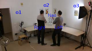
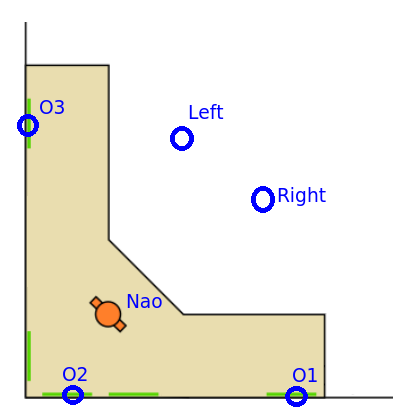
Figure 3: The Vernissage setup. Left: Global view of an “exhibition" showing wall paintings, two participants, i.e. left-p and right-p, and the NAO robot. Right: Top view of the room showing the Vernissage layout.

The scene was recorded with a camera embedded into the robot head and with a VICON motion capture system consisting of a network of infrared cameras, placed onto the walls, and of optical markers, placed onto the robot and people heads. Both were recorded at 25 frames per second (fps). There is a total of ten recordings, each lasting ten minutes. The VICON system provided accurate estimates of head positions, $\hbox to0.0pt{\hskip 1.25pt\leavevmode\hbox{\set@color$\overline{\hbox{}}$}\hss}{\leavevmode\hbox{\set@color$\mathbf{X}$}}_{1:T}$ and head orientations, $\hbox to0.0pt{\hskip 1.25pt\leavevmode\hbox{\set@color$\overline{\hbox{}}$}\hss}{\leavevmode\hbox{\set@color$\mathbf{H}$}}_{1:T}$. Head positions and head orientations were also estimated using from the RGB images gathered with the camera embedded into the robot head. The RGB images are processed as follows. We use the OpenCV version of [36] to detect faces and their bounding boxes which are then tracked over time using [37]. Next, we extract HOG descriptors from each bounding box and apply a head-pose estimator, e.g. [38]. This yields $\tilde{\mathbf{H}}_{1:T}$. The 3D head positions, $\tilde{\mathbf{X}}_{1:T}$, can be estimated using the line of sight through the face center and the bounding-box size, which provides a rough estimate of the depth along the line of sight.

In the remaining of this paper, $\hbox to0.0pt{\hskip 1.25pt\leavevmode\hbox{\set@color$\overline{\hbox{}}$}\hss}{\leavevmode\hbox{\set@color$\mathbf{X}$}}_{1:T}$ and $\hbox to0.0pt{\hskip 1.25pt\leavevmode\hbox{\set@color$\overline{\hbox{}}$}\hss}{\leavevmode\hbox{\set@color$\mathbf{H}$}}_{1:T}$ are referred to as Vicon Data; $\tilde{\mathbf{X}}_{1:T}$ and $\tilde{\mathbf{H}}_{1:T}$ as RGB Data. Because the whole setup was carefully calibrated, both Vicon and RGB Data are represented in the same coordinate frame.

In all our experiments we assumed that the passive targets are static and their positions are provided in advance. The position of the robot itself is also known in advance and one can easily estimate the orientation of the robot head from motor readings. Finally, the VFOAs of the participants were manually annotated in all the frames of all the recordings.

VI-B The LAEO Dataset

The LAEO dataset [4] is an extension of the TVHID (TV Human Interaction Dataset) [39]. It consists of 300 videos extracted from TV shows. At least two actors appear in each video engaged in four human-human interactions: handshake, highfive, hug, and kiss. There are 50 videos for each interaction and 100 videos with no interaction. The videos have been grabbed at 25 fps and each video lasts from five seconds to twenty-five seconds. LAEO is further annotated, namely some of these videos are split into shots which are separated by cuts. There are 443 shots in total which are manually annotated whenever two persons look at each other, [4].

While there is no passive target in this dataset ($M=0$), the number of active targets ($N$) corresponds to the number of persons in each shot. In practice $N$ varies from one to eight persons. All the faces in the dataset are annotated with a bounding box and with a coarse head-orientation label: frontal-right, frontal-left, profile-right, profile-left, backward. As with Vernissage, we use the bounding-box center and size to estimate the 3D coordinates of the heads, $\hbox to0.0pt{\hskip 1.25pt\leavevmode\hbox{\set@color$\overline{\hbox{}}$}\hss}{\leavevmode\hbox{\set@color$\mathbf{X}$}}_{1:T}$. We also assigned a yaw value to each one of the five coarse head orientations, $\hbox to0.0pt{\hskip 1.25pt\leavevmode\hbox{\set@color$\overline{\hbox{}}$}\hss}{\leavevmode\hbox{\set@color$\mathbf{H}$}}_{1:T}$. We also computed finer head orientations, $\tilde{\mathbf{H}}_{1:T}$, using [38].

VI-C Algorithmic Details

The inference procedure is summarized in Algorithm 1. This is basically an iterative filtering procedure. The update step consists of applying the recursive relationship, derived in Section IV, to $\boldsymbol{\mu}_{t}^{ij}$, $\boldsymbol{\Sigma}_{t}^{ij}$ and $c_{t}^{ij}$, using $\boldsymbol{\mu}_{t}^{ijk}$, $\boldsymbol{\Sigma}_{t}^{ijk}$ and $c_{t-1,t}^{ijk}$ as intermediate variables. The VFOA is chosen using MAP, given observations up to the current frame, and the gaze direction is the mean of the filtered distribution (the first two components of $\boldsymbol{\mu}_{t}^{ij}$ are indeed the mean for the pan and tilt gaze angles).

Algorithm 1 Inference

1:procedure GazeAndVFOA

2:     $\mathbf{X}_{1},\mathbf{H}_{1}\leftarrow\textsc{GetObservations}(time=1)$

3:     $c_{1},\boldsymbol{\mu}_{1},\boldsymbol{\Sigma}_{1}\leftarrow\textsc{Initialization}(\mathbf{H}_{1},\mathbf{X}_{1})$

4:     $\mathrm{V}_{1}^{i}\leftarrow\operatorname*{argmax}_{j}c_{1}^{ij}$

5:     $\mathbf{G}_{1}^{i}\leftarrow\boldsymbol{\mu}_{1}^{ij}[1..2]$

6:     for $t=2..T$ do

7:         $\mathbf{X}_{t},\mathbf{H}_{t}\leftarrow\textsc{GetObservations}(time=t)$

8:         $c_{t},\boldsymbol{\mu}_{t},\boldsymbol{\Sigma}_{t}\leftarrow\textsc{Update}(\mathbf{H}_{t},\mathbf{X}_{t},c_{t-1},\boldsymbol{\mu}_{t-1},\boldsymbol{\Sigma}_{t-1})$

9:         $\mathrm{V}_{t}^{i}\leftarrow\operatorname*{argmax}_{j}c_{t}^{ij}$

10:         $\mathbf{G}_{t}^{i}\leftarrow\boldsymbol{\mu}_{t}^{ij}[1..2]$      

11:     return $\mathbf{V}_{1:T},\mathbf{G}_{1:T}$

Let’s now describe the initialization procedure used by Algorithm 2. In a probabilistic framework, parameter intialization is generally addressed by defining an initial distribution, e.g. $P(\mathbf{L}_{1}|\mathbf{V}_{1})$. Here, we did not explicitly define such a distribution. Initialization is based on the fact that, with repeated similar observation inputs, the algorithm reaches a steady-state. The initialization algorithm uses a repeated update method with initial observation to provide an estimate of gaze and of reference directions. Consequently, the initial filtering distribution $P(\mathbf{L}_{1},\mathbf{V}_{1}|\mathbf{H}_{1},\mathbf{X}_{1})$ is implicitly defined as the expected stationary state.

Algorithm 2 Initialization

1:procedure Initialization($\mathbf{H}_{1},\mathbf{X}_{1}$)

2:     $\boldsymbol{\mu}_{in}\leftarrow[\mathbf{H}_{1};\mathbf{0};\mathbf{H}_{1};\mathbf{0}]$

3:     $\boldsymbol{\Sigma}_{in}\leftarrow\mathbf{I}$

4:     $c_{in}\leftarrow\frac{1}{N+M}(\textit{Uniform})$

5:     while Not Convergence do

6:         $c_{in},\boldsymbol{\mu}_{in},\boldsymbol{\Sigma}_{in}\leftarrow\textsc{Update}(\mathbf{H}_{1},\mathbf{X}_{1},c_{in},\boldsymbol{\mu}_{in},\boldsymbol{\Sigma}_{in})$      

7:     return $c_{in},\boldsymbol{\mu}_{in},\boldsymbol{\Sigma}_{in}$

VI-D Algorithm Complexity

The computational complexity of Algorithm 1 is

$$C =T(C_{O}+C_{U})+T_{I}C_{U},$$ (56)

where $T$ is the number of frames in a test video, $T_{I}$ is the number of iterations needed by the Algorithm 2 (initialization) to converge, $C_{O}$ is the computational complexity of GetObservation and $C_{U}$ is the computational complexity of Update. The complexity of one iteration of Algorithm 1 is $C_{O}+C_{U}$. $C_{O}$ depends on face detection and head pose estimation algorithms. Hence we concentrate on $C_{U}$. From Section IV one sees that the following values need to be computed: $P(\mathbf{H}_{t}^{i}|\mathrm{V}_{t}^{i}=j,\mathrm{V}_{t-1}^{i}=k,\mathbf{H}_{1:t-1},\mathbf{X}_{1:t-1})$, $c_{t-1,t}^{ijk}$, $\boldsymbol{\mu}_{t}^{ijk}$, $\boldsymbol{\Sigma}_{t}^{ijk}$, and then $c_{t}^{ij}$, $\boldsymbol{\mu}_{t}^{ij}$ and $\boldsymbol{\Sigma}_{t}^{ij}$, for each active target $i$, and for each combination of targets $j$ and $k$ different from $i$. There are $N$ possible values for $i$ and $(N+M)$ possible values for $j$ and $k$. Then,

$$C_{U}=K\times N(N+M)^{2},$$ (57)

where $K$ is a factor whose complexity can be estimated as follows. The most time-consuming part is the Kalman Filter algorithm used to estimate $\boldsymbol{\mu}_{t}^{ijk}$ and $\boldsymbol{\Sigma}_{t}^{ijk}$ from $\boldsymbol{\mu}_{t}^{ik}$ and $\boldsymbol{\Sigma}_{t}^{ik}$. These calculations are dominated by several 8$\times$8 and 2$\times$8 matrix inversions and multiplications. By neglecting scalar multiplications and matrix additions, and by denoting with $C_{KF}$ the complexity of the Kalman filter, we obtain that $K\approx C_{KF}$ and hence $C_{U}\approx C_{KF}\times N(N+M)^{2}$.

VII Experimental results

VII-A Vernissage Dataset

We applied the same experimental protocol to the Vicon and RGB data. We used a leave-one-video-out strategy for training. The test is performed on the left out video. We used the frame recognition rate (FRR) metrics to quantitatively evaluate the methods. FRR computes the percentage of frames for which the VFOA is correctly estimated. One should note however that the ground-truth VFOAs were obtained by manually annotating each frame in the data. This is subject to errors since the annotator has to associate a target with each person.

The VFOA transition probabilities and the model parameters were estimated using the learning method described in Section V. Appendix B provides the formulas used for estimating the VFOA transition probabilities given the annotated data. Notice that the fifteen transitions probabilities thus estimated are identical for both data, Vicon and RGB.

The Gaussian parameters, i.e. (35), were estimated using the EM algorithm of Section V-B. This learning procedure requires head-pose estimates as well as the targets locations, estimated as just explained. Since these estimates are different for the two kinds of data (Vicon and RGB) we carried out the learning process twice, with the Vicon data and with the RGB data. The EM algorithm needs initialization. The initial parameter values for $\boldsymbol{\alpha}$ and $\boldsymbol{\beta}$ are $\boldsymbol{\alpha}^{0}=\boldsymbol{\beta}^{0}=\operatorname{Diag\,}(0.5,0.5)$. Matrices $\boldsymbol{\Sigma}_{\mathbf{H}}$ and $\boldsymbol{\Gamma}_{\mathbf{L}}$ defined in (20) are initialized with isotropic covariances: $\boldsymbol{\Sigma}_{\mathbf{H}}^{0}=\sigma\mathbf{I}_{2}$, $\boldsymbol{\Gamma}_{\mathbf{G}}^{0}=\boldsymbol{\Gamma}_{\dot{\mathbf{G}}}^{0}=\gamma\mathbf{I}_{2}$, and $\boldsymbol{\Gamma}_{\mathbf{R}}^{0}=\boldsymbol{\Gamma}_{\dot{\mathbf{R}}}^{0}=\eta\mathbf{I}_{2}$ with $\sigma=15$, $\gamma=5$, and $\eta=0.5$. In particular, this initialization is consistent with (12). In practice we noticed that the covariances estimated by training remain consistent with (12).

VII-B Results with Vicon Data

The FRR of the estimated VFOAs for the Vicon data are summarized in Table I. A few examples are shown in Figure 5.

Table I: FRR scores of the estimated VFOAs for the Vicon data for the left and right persons (left-p and right-p).

Recording	Ba & Odobez [26]		Proposed
	left-p	right-p	left-p	right-p
09	51.6	65.1	59.8	61.4
10	64.3	74.4	76.5	65.0
12	53.5	67.6	61.6	63.2
15	67.1	46.2	64.8	67.6
18	37.5	28.3	62.0	53.7
19	56.7	45.4	54.5	60.4
24	44.9	49.0	59.7	54.7
26	40.3	32.9	43.6	43.1
27	65.8	72.0	79.8	78.3
30	69.1	49.1	72.0	63.9
Mean	54.5		62.6

The FRR score varies between $28.3\%$ and $74.4\%$ for [26] and between $43.1\%$ and $79.8\%$ for the proposed method. Notice that high scores are obtained by both methods for recording #27. Similarly, low scores are obtained for recording #26. Since both methods assume that head motions and gaze shifts occur synchronously, an explanation could be that this hypothesis is only valid for some of the participants. The confusion matrices for VFOA classification using Vicon data are given in Figure 4.

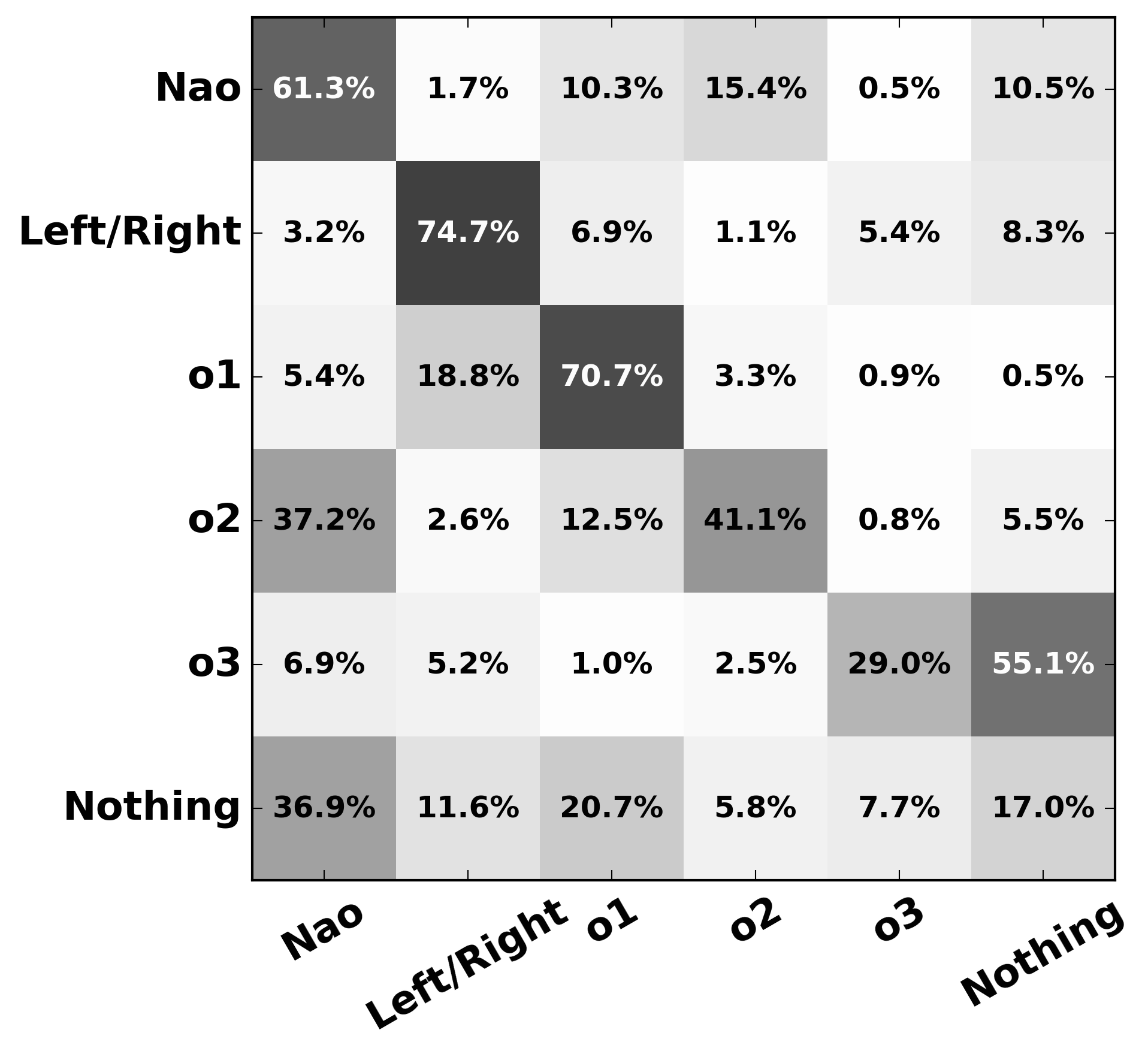
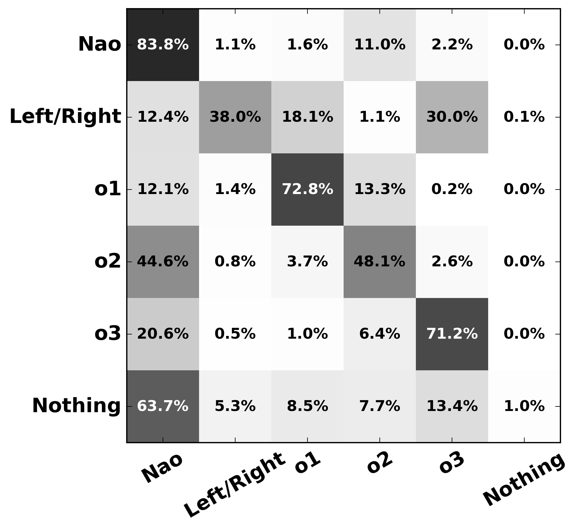
Figure 4: Confusion matrices for the Vicon data. Left: [26]. Right: Proposed algorithm. Row-wise: ground-truth VFOAs. Column-wise: estimated VFOAs. Diagonal terms represent the recall.

There are a few similarities between the results obtained with the two methods. In particular, wall painting #$o_{2}$ stands just behind Nao and both methods don’t always discriminate between these two targets. In addition, the head of one of the persons is often aligned with painting #$o_{1}$ from the viewpoint of the other person. A similar remark holds for painting #$o_{3}$. As a consequence both methods often confuse the VFOA in these cases. This can be seen in the third image of Figure 5. Indeed, it is difficult to estimate whether the left person (left-p) looks at #$o_{1}$ or at right-p.

Finally, both methods have problems with recognizing the VFOA “nothing” or gaze aversion ($\mathrm{V}_{t}^{i}=0$). We propose the following explanation: the targets are widespread in the scene, hence it is likely that an acceptable target lies in most of the gaze directions. Moreover, Nao is centrally positioned, therefore the head orientation used to look at Nao is similar to the resting head orientation used for gaze aversion. However, in [26] the reference head orientation is fixed and poorly suited for dynamic head-to-gaze mapping, hence the high error rate on painting #$o_{3}$. Our method favors the selection of a target, either active or passive, over the no target (nothing) case.

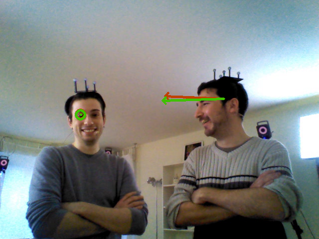
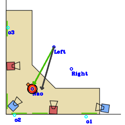
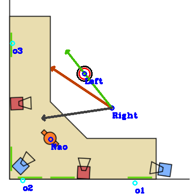
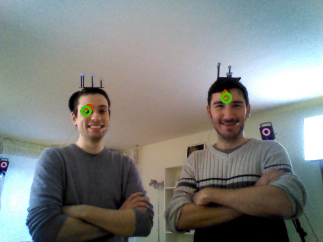
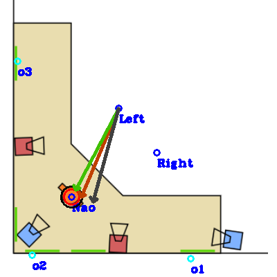
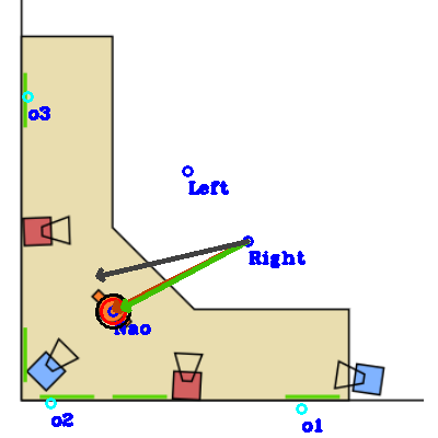
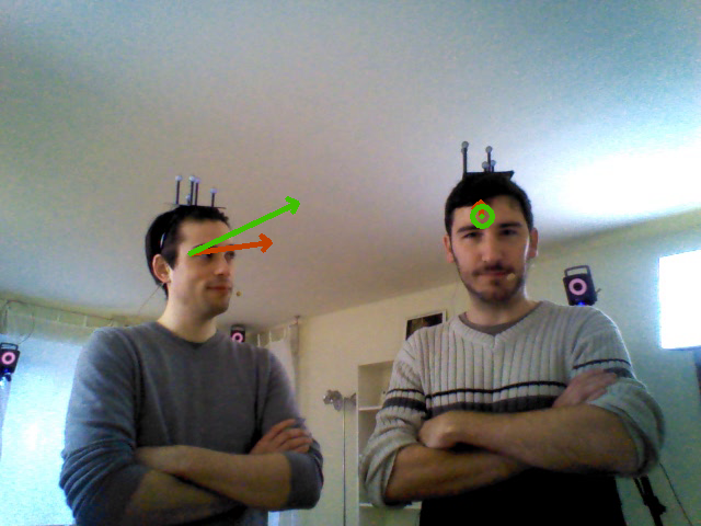
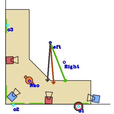
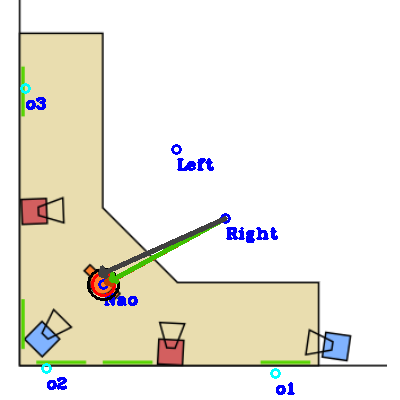
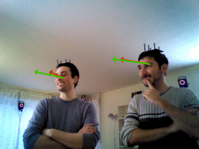
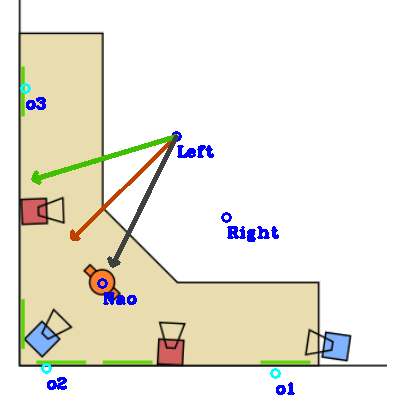
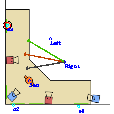
Figure 5: Results obtained with the proposed method on Vicon data. Gaze directions are shown with green arrows, head reference directions with dark-grey arrows and observed head directions with red arrows. The ground-truth VFOA is shown with a black circle. The top row displays the image of the robot-head camera. Top views of the room show results obtained for the left-p (middle row) and for the right-p (bottom row). In the last example the left-p gazes at “nothing".

VII-C Results with RGB Data

The RGB images were processed as described in section VI-A above in order to obtain head orientations, $\tilde{\mathbf{H}}_{1:T}$, and 3D head positions, $\tilde{\mathbf{X}}_{1:T}$. Table II shows the accuracy of these measurements (in degrees and in centimeters), when compared with the ground truth provided by the Vicon motion capture system. As it can be seen, while the head orientation estimates are quite accurate, the error in estimating the head positions can be as large as 0.8 m for participants lying in between 1.5 m and 2.5 m in front of a robot, e.g. recordings #19 and #24. In particular this error increases as a participant is farther away from the robot. In these cases, the bounding box is larger than it should be and hence the head position is, on an average, one meter closer than the true position. These relatively large errors in 3D head position affect the overall behavior of the algorithm.

Table II: Mean error for head pose estimations from RGB data, for the left person (left-p) and the right person (right-p). The errors in head position (centimeters) and orientation (degrees) are computed with respect to values provided by the motion capture system.

Video	Position error (cm)		Pan error		Tilt error
	left-p	right-p	left-p	right-p	left-p	right-p
09	18.1	20.8	4.4°	4.8°	3.7°	3.2°
12	35.7	41.5	4.8°	5.5°	2.6°	3.8°
18	36.9	12.8	6.8°	3.7°	5.8°	2.5°
19	86.0	87.4	4.0°	5.8°	2.7°	3.7°
24	86.5	73.9	3.3°	3.5°	2.8°	2.7°
26	50.2	56.9	7.4°	9.0°	4.1°	5.2°
27	64.5	58.3	4.1°	5.8°	3.2°	4.4°
30	16.7	13.3	2.8°	2.9°	1.8°	2.7°
Mean	46.4		5.0°		3.3°

Table III: FRR scores of the estimated VFOAs obtained with [26] and with the proposed method for the RGB data. The last two columns show the 3D head position errors of Table II.

Video	Ba & Odobez [26]		Proposed		Head pos. error
	left-p	right-p	left-p	right-p	left-p	right-p
09	50.3	59.8	58.1	55.9	18.1	20.8
12	54.2	14.8	59.0	46.5	35.7	41.5
18	39.0	16.1	64.2	33.1	36.9	12.8
27	38.2	17.1	53.3	55.1	64.5	58.3
30	61.6	44.6	54.7	66.6	16.7	13.3
Mean	39.0		54.7

The FRR scores obtained with the RGB data are shown in Table III. As expected the loss in accuracy is correlated with the head position error: the results obtained with recordings #09 and #30 are close to the ones obtained with the Vicon data, whereas there is a significant loss in accuracy for the other recordings. The loss is notable for [26] in the case of the right person (right-p) for the recordings #12, #18 and #27. The confusion matrices obtained with the RGB data are shown on Fig. 6.

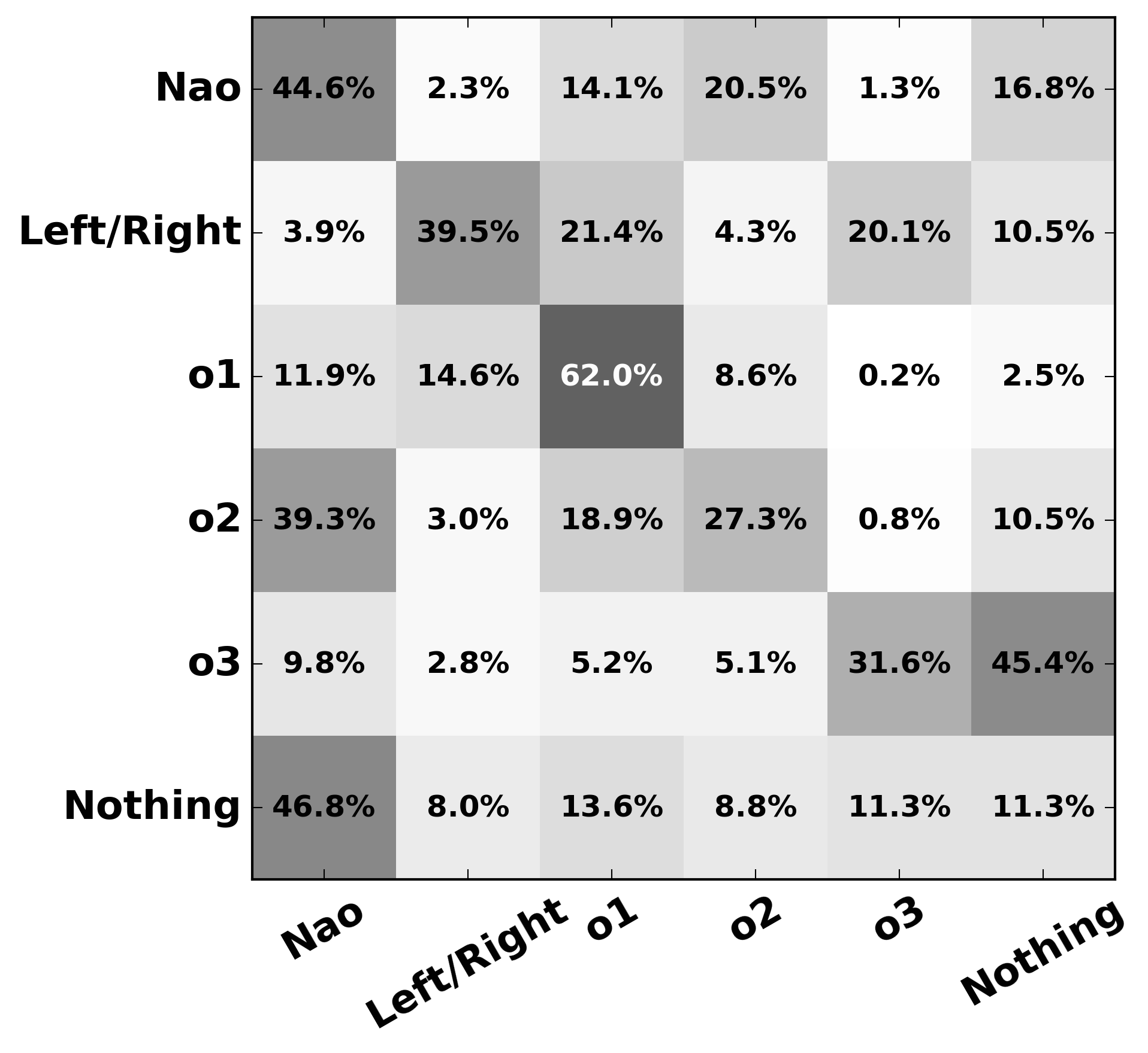
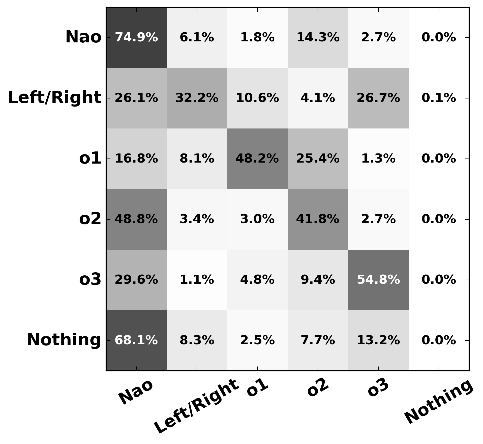
Figure 6: Confusion matrices for the RGB data. Left: [26]. Right: Proposed algorithm. Row-wise: ground-truth VFOAs. Column-wise: estimated VFOAs. Diagonal terms represent the recall.

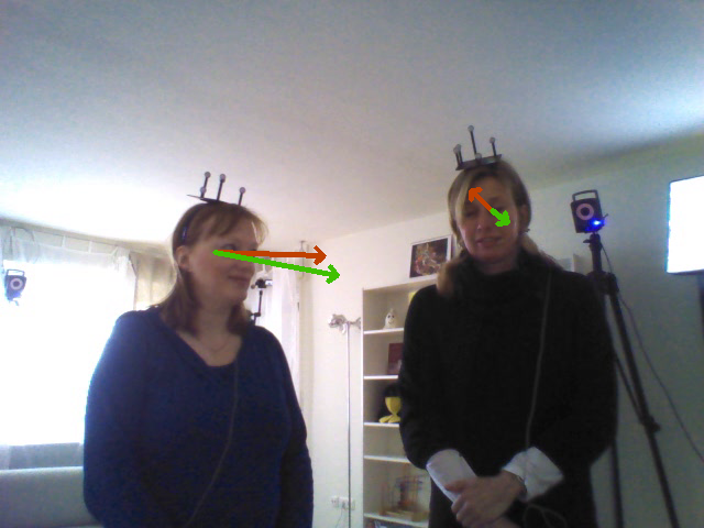
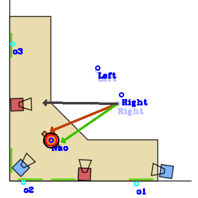
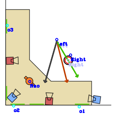
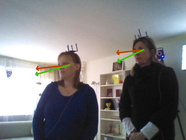
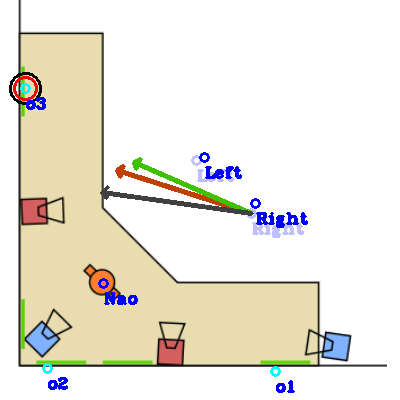
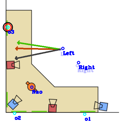
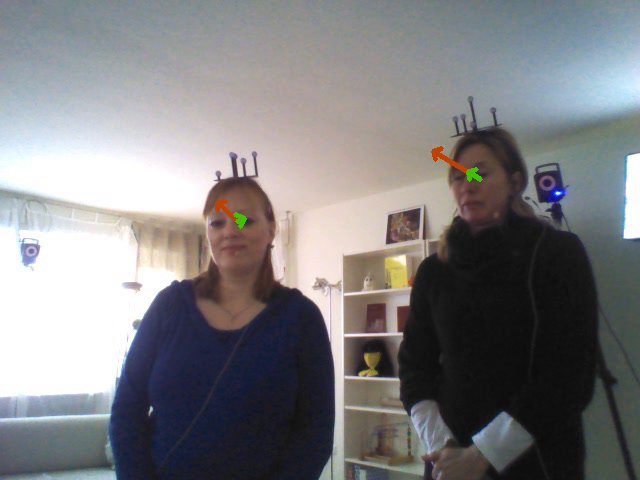
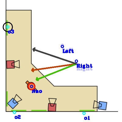
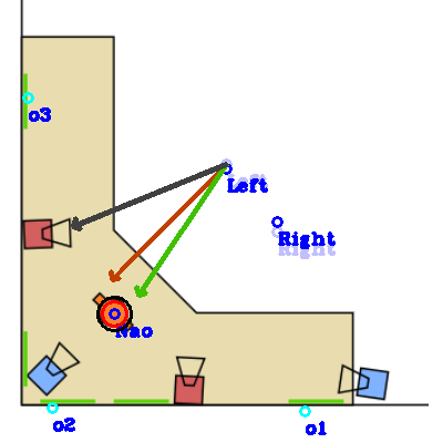
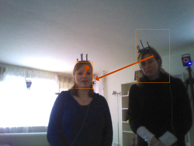
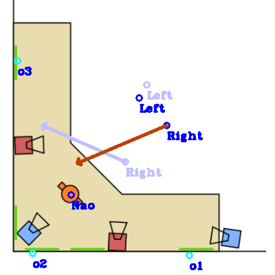
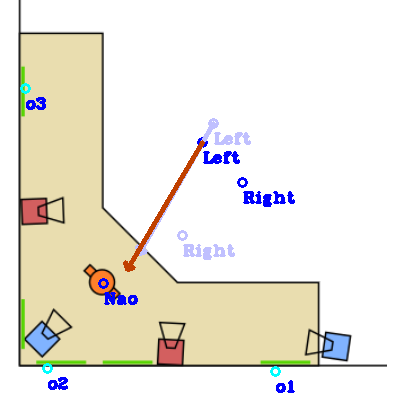
Figure 7: Results obtained with the proposed method on RGB data. Gaze directions are shown with green arrows, head reference directions with dark-grey arrows and observed head directions with red arrows. The ground-truth VFOA is shown with a black circle. The top row displays the image of the robot-head camera. Top views of the room show results obtained for the left person (left-p, middle row) and the right person (right-p, bottom row).

In the case of RGB data, the comparison between our method and the method of [31] is biased by the use of different head orientation and 3D head position estimators. Indeed, the RGB data results reported in [31] were obtained with unpublished methods for estimating head orientations and 3D head positions, and for head tracking. Moreover, [31] uses cross-modal information, namely the speaker identity based on the audio track (one of the participants or the robot) as well as the identity of the object of interest. We also note that [31] reports mean FRR values obtained over all the test recordings, instead of an FRR value for each recording. Table IV summarizes a comparison between the average FRR obtained with our method, with [26], and with [31]. Our method yields a similar FRR score as [31] using the Vicon data (first row) in which case the same head pose inputs are used.

Table IV: Mean FRR scores obtained with [26], with [31] and with the proposed method. Recording #26 was excluded from the FRR means as reported in [31]. Moreover, [31] uses additional contextual information.

	Ba & Odobez [26]	Sheikhi [31]	Proposed
Vicon data	56.5	66.6	64.7
RGB data	39.0	62.4	54.7

VII-D LAEO Dataset

As already mentioned in Section VI-B above, the LAEO annotations are incomplete to estimate the person-wise VFOA at each frame. Indeed, the only VFOA-related annotation is whether two people are looking at each other during the shot. This is not sufficient to know in which frames they are actually looking at each other. Moreover, when more than two people appear in a shot, the annotations don’t specify who are the people that look at each other. For these reasons, we decided to estimate the parameters using Vicon data of the whole Vernissage dataset, i.e. cross-validation.

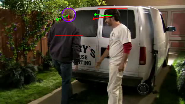
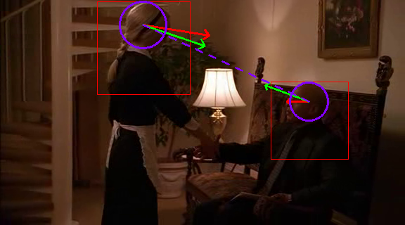
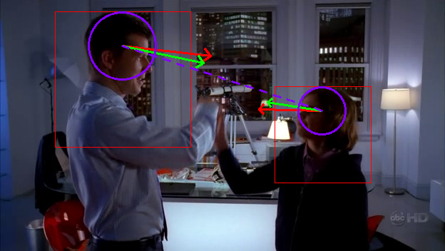
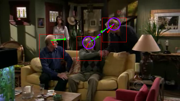
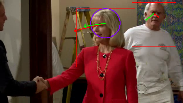
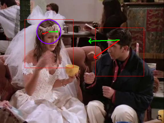
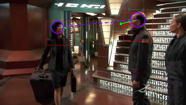
Figure 8: This figure shows some results obtained with the LAEO dataset. The top row shows results obtained with coarse head orientation and the bottom row shows results obtained with fine head orientation. Head orientations are shown with red arrows. The algorithm infers gaze directions (green arrows) and VFOAs (blue circles). People looking at each others are shown with a dashed blue line.

We used the same pipeline as with the Vernissage RGB data to estimate 3D head positions, $\tilde{\mathbf{X}}_{1:T}$, from the face bounding boxes. Concerning head orientation, there are two cases: coarse head orientations (manually annotated) and fine head orientations (estimated). Coarse head orientations were obtained in the following way: pan and tilt values were associated with each head orientation label, namely the pan angles $-20\degree$, $20\degree$, $-80\degree$, $80\degree$, and $180\degree$ were assigned to labels frontal-left, frontal-right, profile-left, profile-right, and backwards respectively, while a tilt anble of $0\degree$ was assigned to all five labels. Fine head orientations were estimated using the same procedure as in the case of the Vernissage RGB data, namely face detection, face tracking, and head orientation estimation using [38]. Algorithm 1 was used to compute the VFOA for each frame and for each person thus allowing to determine who looks at whom, e.g. Fig. 8.

We used two shot-wise, not frame-wise, metrics since the LAEO annotations are for each shot: the shot recognition rate (SRR), e.g. Table V, and the average precision (AP), e.g. Table VI. We note that [4] only provides AP scores. It is interesting to note that the proposed method yields results comparable with those of [4] on this dataset. This is quite remarkable knowing that we estimated the model parameters with the Vernissage training data.

Table V: Average shot recognition rate (SRR) obtained with [26] and with the proposed method.

	Ba & Odobez [26]	Proposed
Coarse head orientation	0.535	0.727
Fine head orientation	0.363	0.479

Table VI: Average precision (AP) obtained with [4], with Ba & Odobez [26] and with the proposed method.

	Marin-Jimenez et al. [4]	[26]	Proposed
Coarse head orientation	0.925	0.916	0.923
Fine head orientation	0.896	0.838	0.890

VIII Conclusions

In this paper we addressed the problem of estimating and tracking gaze and visual focus of attention of a group of participants involved in social interaction. We proposed a Bayesian dynamic formulation that exploits the correlation between head movements and eye gaze on one side, and between visual focus of attention and eye gaze on the other side. We described in detail the proposed model. In particular we showed that the entries of the large-sized matrix of VFOA transition probabilities have a very small number of different possibilities for which we provided closed-form formulae. The immediate consequence of this simplified transition matrix is that the associated learning doesn’t require a large training dataset. We showed that the problem of simultaneously inferring VFOAs and gaze directions over time can be cast in the framework of a switching state-space model, which yields tractable learning and inference algorithms.

We applied the proposed method to two datasets, Vernissage and LAEO. Vernissage contains several recordings of a human-robot interaction scenario. We experimented both with motion capture data gathered with a Vicon system and with RGB data gathered with a camera mounted onto a robot head. We also experimented with the LAEO dataset that contains several hundreds of video shots extracted from TV shows. A quite remarkable result is that the parameters obtained by training the model with the Vernissage data have been successfully used for testing the method with the LAEO data, i.e. cross-validation. This can be explained by the fact that social interactions, even in different contexts, share a lot of characteristics. We compared our method with three other methods, based on HMMs [26], on input-output HMMs [31], and on a geometric model [4]. The interest of these methods (including ours) resides in the fact that eye detection, unlike many existing gaze estimation methods, is not needed. This feature makes the above methods practical and effective in a very large number of situations, e.g. social interaction.

We note that gaze inference from head orientation is an ill-posed problem. Indeed, the correlation between gaze and head movements is person dependent as well as context dependent. It is however important to detect gaze whenever the eyes cannot be reliably extracted from images and properly analyzed. We proposed to solve the problem based on the fact that alignments often occur between gaze directions and a finite number of targets, which is a sensible assumption in practice.

Contextual information could considerably improve the results. Indeed, additional information such as speaker recognition (as in [31]), speaker localization [40], speech recognition, or speech-turn detection [41] may be used to learn VFOA transitions in multi-party multimodal dialog systems.

In the future we plan to investigate discriminative methods based on neural network architectures for inferring gaze directions from head orientations and from contextual information. For example one could train a deep learning network from input-output pairs of head pose and visual focus of attention. For this purpose, one can combine a multiple-camera system, to accurately detect the eyes of several participants and to estimate their head poses, with a microphone-array and associated algorithms to infer speaker and speech information.

Appendix A VFOA Transition Probabilities

Using the notations introduced in section  III-C, let $i$, $1\leq i\leq N$, be an active target. In section  III-C we showed that in practice the probability transition matrix has up to 15 different entries. For completeness, these entries are listed below.

• The VFOA of $i$ at $t-1$ is neither an active nor a passive target ($k=0$):

  $$p_{1}= P(\mathrm{V}_{t}^{i}=0|\mathrm{V}_{t-1}^{i}=0)$$

  $$p_{2}= P(\mathrm{V}_{t}^{i}=j|\mathrm{V}_{t-1}^{i}=0)$$

• The VFOA of $i$ at $t-1$ is a passive target ($N<k\leq N+M$):

  $$p_{3}= P(\mathrm{V}_{t}^{i}=0|\mathrm{V}_{t-1}^{i}=k)$$

  $$p_{4}= P(\mathrm{V}_{t}^{i}=k|\mathrm{V}_{t-1}^{i}=k)$$

  $$p_{5}= P(\mathrm{V}_{t}^{i}=j|\mathrm{V}_{t-1}^{i}=k)$$

• The VFOA of $i$ at $t-1$ is an active target ($1\leq k\leq N,k\neq i$):

  $$p_{6}= P(\mathrm{V}_{t}^{i}=0|\mathrm{V}_{t-1}^{i}=k,\mathrm{V}_{t-1}^{k}=0)$$

  $$p_{7}= P(\mathrm{V}_{t}^{i}=k|\mathrm{V}_{t-1}^{i}=k,\mathrm{V}_{t-1}^{k}=0)$$

  $$p_{8}= P(\mathrm{V}_{t}^{i}=j|\mathrm{V}_{t-1}^{i}=k,\mathrm{V}_{t-1}^{k}=0)$$

  $$p_{9}= P(\mathrm{V}_{t}^{i}=0|\mathrm{V}_{t-1}^{i}=k,\mathrm{V}_{t-1}^{k}=i)$$

  $$p_{10}= P(\mathrm{V}_{t}^{i}=k|\mathrm{V}_{t-1}^{i}=k,\mathrm{V}_{t-1}^{k}=i)$$

  $$p_{11}= P(\mathrm{V}_{t}^{i}=j|\mathrm{V}_{t-1}^{i}=k,\mathrm{V}_{t-1}^{k}=i)$$

  $$p_{12}= P(\mathrm{V}_{t}^{i}=0|\mathrm{V}_{t-1}^{i}=k,\mathrm{V}_{t-1}^{k}=l)$$

  $$p_{13}= P(\mathrm{V}_{t}^{i}=k|\mathrm{V}_{t-1}^{i}=k,\mathrm{V}_{t-1}^{k}=l)$$

  $$p_{14}= P(\mathrm{V}_{t}^{i}=l|\mathrm{V}_{t-1}^{i}=k,\mathrm{V}_{t-1}^{k}=l)$$

  $$p_{15}= P(\mathrm{V}_{t}^{i}=j|\mathrm{V}_{t-1}^{i}=k,\mathrm{V}_{t-1}^{k}=l)$$

Appendix B VFOA Learning

This appendix provides the formulae allowing to estimate the 15 transitions probabilities as explained in section V-A.

$$\hat{p}_{1}= \frac{\displaystyle\sum_{q=1}^{Q}\sum_{i=2}^{N_{q}}\sum_{t=2}^{T_{q}}\delta_{0}(\mathrm{V}_{t}^{q,i})\delta_{0}(\mathrm{V}_{t-1}^{q,i})}{\displaystyle\sum_{q=1}^{Q}\sum_{i=2}^{N_{q}}\sum_{t=2}^{T_{q}}\delta_{0}(\mathrm{V}_{t-1}^{q,i})}$$

$$\hat{p}_{2}= \frac{\displaystyle\sum_{q=1}^{Q}\sum_{i=2}^{N_{q}}\sum_{t=2}^{T_{q}}\sum_{j\neq i}\delta_{j}(\mathrm{V}_{t}^{q,i})\delta_{0}(\mathrm{V}_{t-1}^{q,i})}{\displaystyle\sum_{q=1}^{Q}\sum_{i=2}^{N_{q}}\sum_{t=2}^{T_{q}}\delta_{0}(\mathrm{V}_{t-1}^{q,i})}$$

$$\hat{p}_{3}= \frac{\displaystyle\sum_{q=1}^{Q}\sum_{i=2}^{N_{q}}\sum_{t=2}^{T_{q}}\sum_{k=N_{q}+1}^{N_{q}+M_{q}}\delta_{0}(\mathrm{V}_{t}^{q,i})\delta_{k}(\mathrm{V}_{t-1}^{q,i})}{\displaystyle\sum_{q=1}^{Q}\sum_{i=2}^{N_{q}}\sum_{t=2}^{T_{q}}\sum_{k=N_{q}+1}^{N_{q}+M_{q}}\delta_{k}(\mathrm{V}_{t-1}^{q,i})}$$

$$\hat{p}_{4}= \frac{\displaystyle\sum_{q=1}^{Q}\sum_{i=2}^{N_{q}}\sum_{t=2}^{T_{q}}\sum_{k=N_{q}+1}^{N_{q}+M_{q}}\delta_{k}(\mathrm{V}_{t}^{q,i})\delta_{k}(\mathrm{V}_{t-1}^{q,i})}{\displaystyle\sum_{q=1}^{Q}\sum_{i=2}^{N_{q}}\sum_{t=2}^{T_{q}}\sum_{k=N_{q}+1}^{N_{q}+M_{q}}\delta_{k}(\mathrm{V}_{t-1}^{q,i})}$$

$$\hat{p}_{5}= \frac{\displaystyle\sum_{q=1}^{Q}\sum_{i=2}^{N_{q}}\sum_{t=2}^{T_{q}}\sum_{k=N_{q}+1}^{N_{q}+M_{q}}\sum_{j\neq i,k}\delta_{j}(\mathrm{V}_{t}^{q,i})\delta_{k}(\mathrm{V}_{t-1}^{q,i})}{\displaystyle\sum_{q=1}^{Q}\sum_{i=2}^{N_{q}}\sum_{t=2}^{T_{q}}\sum_{k=N_{q}+1}^{N_{q}+M_{q}}\delta_{k}(\mathrm{V}_{t-1}^{q,i})}$$

$$\hat{p}_{6}= \frac{\displaystyle\sum_{q=1}^{Q}\sum_{i=2}^{N_{q}}\sum_{t=2}^{T_{q}}\sum_{\begin{subarray}{c}k=1\\ k\neq i\end{subarray}}^{N_{q}}\delta_{0}(\mathrm{V}_{t}^{q,i})\delta_{k}(\mathrm{V}_{t-1}^{q,i})\delta_{0}(\mathrm{V}_{t-1}^{q,k})}{\displaystyle\sum_{q=1}^{Q}\sum_{i=2}^{N_{q}}\sum_{t=2}^{T_{q}}\sum_{\begin{subarray}{c}k=1\\ k\neq i\end{subarray}}^{N_{q}}\delta_{k}(\mathrm{V}_{t-1}^{q,i})\delta_{0}(\mathrm{V}_{t-1}^{q,k})}$$

$$\hat{p}_{7}= \frac{\displaystyle\sum_{q=1}^{Q}\sum_{i=2}^{N_{q}}\sum_{t=2}^{T_{q}}\sum_{\begin{subarray}{c}k=1\\ k\neq i\end{subarray}}^{N_{q}}\delta_{k}(\mathrm{V}_{t}^{q,i})\delta_{k}(\mathrm{V}_{t-1}^{q,i})\delta_{0}(\mathrm{V}_{t-1}^{q,k})}{\displaystyle\sum_{q=1}^{Q}\sum_{i=2}^{N_{q}}\sum_{t=2}^{T_{q}}\sum_{\begin{subarray}{c}k=1\\ k\neq i\end{subarray}}^{N_{q}}\delta_{k}(\mathrm{V}_{t-1}^{q,i})\delta_{0}(\mathrm{V}_{t-1}^{q,k})}$$

$$\hat{p}_{8}= \frac{\displaystyle\sum_{q=1}^{Q}\sum_{i=2}^{N_{q}}\sum_{t=2}^{T_{q}}\sum_{\begin{subarray}{c}k=1\\ k\neq i\end{subarray}}^{N_{q}}\sum_{j\neq i,k}\delta_{j}(\mathrm{V}_{t}^{q,i})\delta_{k}(\mathrm{V}_{t-1}^{q,i})\delta_{0}(\mathrm{V}_{t-1}^{q,k})}{\displaystyle\sum_{q=1}^{Q}\sum_{i=2}^{N_{q}}\sum_{t=2}^{T_{q}}\sum_{\begin{subarray}{c}k=1\\ k\neq i\end{subarray}}^{N_{q}}\delta_{k}(\mathrm{V}_{t-1}^{q,i})\delta_{0}(\mathrm{V}_{t-1}^{q,k})}$$

$$\hat{p}_{9}= \frac{\displaystyle\sum_{q=1}^{Q}\sum_{i=2}^{N_{q}}\sum_{t=2}^{T_{q}}\sum_{\begin{subarray}{c}k=1\\ k\neq i\end{subarray}}^{N_{q}}\delta_{0}(\mathrm{V}_{t}^{q,i})\delta_{k}(\mathrm{V}_{t-1}^{q,i})\delta_{i}(\mathrm{V}_{t-1}^{q,k})}{\displaystyle\sum_{q=1}^{Q}\sum_{i=2}^{N_{q}}\sum_{t=2}^{T_{q}}\sum_{\begin{subarray}{c}k=1\\ k\neq i\end{subarray}}^{N_{q}}\delta_{k}(\mathrm{V}_{t-1}^{q,i})\delta_{i}(\mathrm{V}_{t-1}^{q,k})}$$

$$\hat{p}_{10}= \frac{\displaystyle\sum_{q=1}^{Q}\sum_{i=2}^{N_{q}}\sum_{t=2}^{T_{q}}\sum_{\begin{subarray}{c}k=1\\ k\neq i\end{subarray}}^{N_{q}}\delta_{k}(\mathrm{V}_{t}^{q,i})\delta_{k}(\mathrm{V}_{t-1}^{q,i})\delta_{i}(\mathrm{V}_{t-1}^{q,k})}{\displaystyle\sum_{q=1}^{Q}\sum_{i=2}^{N_{q}}\sum_{t=2}^{T_{q}}\sum_{\begin{subarray}{c}k=1\\ k\neq i\end{subarray}}^{N_{q}}\delta_{k}(\mathrm{V}_{t-1}^{q,i})\delta_{i}(\mathrm{V}_{t-1}^{q,k})}$$

$$\hat{p}_{11}= \frac{\displaystyle\sum_{q=1}^{Q}\sum_{i=2}^{N_{q}}\sum_{t=2}^{T_{q}}\sum_{\begin{subarray}{c}k=1\\ k\neq i\end{subarray}}^{N_{q}}\sum_{j\neq i,k}\delta_{j}(\mathrm{V}_{t}^{q,i})\delta_{k}(\mathrm{V}_{t-1}^{q,i})\delta_{i}(\mathrm{V}_{t-1}^{q,k})}{\displaystyle\sum_{q=1}^{Q}\sum_{i=2}^{N_{q}}\sum_{t=2}^{T_{q}}\sum_{\begin{subarray}{c}k=1\\ k\neq i\end{subarray}}^{N_{q}}\delta_{k}(\mathrm{V}_{t-1}^{q,i})\delta_{i}(\mathrm{V}_{t-1}^{q,k})}$$

$$\hat{p}_{12}= \frac{\displaystyle\sum_{q=1}^{Q}\sum_{i=2}^{N_{q}}\sum_{t=2}^{T_{q}}\sum_{\begin{subarray}{c}k=1\\ k\neq i\end{subarray}}^{N_{q}}\sum_{l\neq i,k}\delta_{0}(\mathrm{V}_{t}^{q,i})\delta_{k}(\mathrm{V}_{t-1}^{q,i})\delta_{l}(\mathrm{V}_{t-1}^{q,k})}{\displaystyle\sum_{q=1}^{Q}\sum_{i=2}^{N_{q}}\sum_{t=2}^{T_{q}}\sum_{\begin{subarray}{c}k=1\\ k\neq i\end{subarray}}^{N_{q}}\sum_{l\neq i,k}\delta_{k}(\mathrm{V}_{t-1}^{q,i})\delta_{l}(\mathrm{V}_{t-1}^{q,k})}$$

$$\hat{p}_{13}= \frac{\displaystyle\sum_{q=1}^{Q}\sum_{i=2}^{N_{q}}\sum_{t=2}^{T_{q}}\sum_{\begin{subarray}{c}k=1\\ k\neq i\end{subarray}}^{N_{q}}\sum_{l\neq i,k}\delta_{k}(\mathrm{V}_{t}^{q,i})\delta_{k}(\mathrm{V}_{t-1}^{q,i})\delta_{l}(\mathrm{V}_{t-1}^{q,k})}{\displaystyle\sum_{q=1}^{Q}\sum_{i=2}^{N_{q}}\sum_{t=2}^{T_{q}}\sum_{\begin{subarray}{c}k=1\\ k\neq i\end{subarray}}^{N_{q}}\sum_{l\neq i,k}\delta_{k}(\mathrm{V}_{t-1}^{q,i})\delta_{l}(\mathrm{V}_{t-1}^{q,k})}$$

$$\hat{p}_{14}= \frac{\displaystyle\sum_{q=1}^{Q}\sum_{i=2}^{N_{q}}\sum_{t=2}^{T_{q}}\sum_{\begin{subarray}{c}k=1\\ k\neq i\end{subarray}}^{N_{q}}\sum_{l\neq i,k}\delta_{l}(\mathrm{V}_{t}^{q,i})\delta_{k}(\mathrm{V}_{t-1}^{q,i})\delta_{l}(\mathrm{V}_{t-1}^{q,k})}{\displaystyle\sum_{q=1}^{Q}\sum_{i=2}^{N_{q}}\sum_{t=2}^{T_{q}}\sum_{\begin{subarray}{c}k=1\\ k\neq i\end{subarray}}^{N_{q}}\sum_{l\neq i,k}\delta_{k}(\mathrm{V}_{t-1}^{q,i})\delta_{l}(\mathrm{V}_{t-1}^{q,k})}$$

$$\hat{p}_{15}= \frac{\displaystyle\sum_{q=1}^{Q}\sum_{i=2}^{N_{q}}\sum_{t=2}^{T_{q}}\sum_{\begin{subarray}{c}k=1\\ k\neq i\end{subarray}}^{N_{q}}\sum_{l\neq i,k}\sum_{j\neq i,k,l}\delta_{j}(\mathrm{V}_{t}^{q,i})\delta_{k}(\mathrm{V}_{t-1}^{q,i})\delta_{l}(\mathrm{V}_{t-1}^{q,k})}{\displaystyle\sum_{q=1}^{Q}\sum_{i=2}^{N_{q}}\sum_{t=2}^{T_{q}}\sum_{\begin{subarray}{c}k=1\\ k\neq i\end{subarray}}^{N_{q}}\sum_{l\neq i,k}\delta_{k}(\mathrm{V}_{t-1}^{q,i})\delta_{l}(\mathrm{V}_{t-1}^{q,k})}$$

Benoit Massé received the M.Eng. degree in applied mathematics and computer science from ENSIMAG, Institut National Polytechnique de Grenoble, France, in 2013, and the M.Sc. degree in graphics, vision and robotics from Université Joseph Fourier, Grenoble, France, in 2014. Currently he is a PhD student in the PERCEPTION team at INRIA Grenoble Rhone-Alpes. His research interests include scene understanding, machine learning and computer vision, with special emphasis on attention recognition for human-robot interaction.

Silèye Ba received the M.Sc. (2000) in applied mathematics and signal processing from University of Dakar, Dakar, Senegal, and the M.Sc. (2002) in mathematics, computer vision, and machine learning from Ecole Normale Supérieure de Cachan, Paris, France. From 2003 to 2009 he was a PhD student and then a post-doctoral researcher at IDIAP Research Institute, Martigny, Switzerland, where he worked on probabilistic models for object tracking and human activity recognition. From 2009 to 2013, he was a researcher at Telecom Bretagne, Brest, France working on variational models for multi-modal geophysical data processing. From 2013 to 2014 he worked at RN3D Innovation Lab, Marseille, France, as a research engineer, where he used computer vision and machine learning principles and methods to develop human-computer interaction software tools. From 2014 to 2016 he was a researcher in the PERCEPTION team at INRIA Grenoble Rhône-Alpes, working on machine learning and computer vision models for human-robot interaction. Since May 2016 he is a computer vision scientist with VideoStitch, Paris.

Radu Horaud received the B.Sc. degree in Electrical Engineering, the M.Sc. degree in Control Engineering, and the Ph.D. degree in Computer Science from the Institut National Polytechnique de Grenoble, France. In 1982-1984 he was a post-doctoral fellow with the Artificial Intelligence Center, SRI International, Menlo Park, CA. Currently he holds a position of director of research with INRIA Grenoble Rhône-Alpes, where he is the founder and head of the PERCEPTION team. His research interests include computer vision, machine learning, audio signal processing, audiovisual analysis, and robotics. Radu Horaud and his collaborators received numerous best paper awards. He is an area editor of the Elsevier Computer Vision and Image Understanding, a member of the advisory board of the Sage International Journal of Robotics Research, and an associate editor of the Kluwer International Journal of Computer Vision. He was program co-chair of IEEE ICCV’01 and of ACM ICMI’15. In 2013, Radu Horaud was awarded an ERC Advanced Grant for his project Vision and Hearing in Action (VHIA) and in 2017 he was awarded an ERC Proof of Concept Grant for this project VHIALab.

References

- [1] E. G. Freedman and D. L. Sparks, “Eye-head coordination during head-unrestrained gaze shifts in rhesus monkeys,” Journal of Neurophysiology, 1997.
- [2] E. G. Freedman, “Coordination of the eyes and head during visual orienting,” Experimental Brain Research, vol. 190, 2008.
- [3] D. B. Jayagopi et al., “The vernissage corpus: A multimodal human-robot-interaction dataset,” IDIAP, Tech. Rep., 2012.
- [4] M. J. Marin-Jimenez, A. Zisserman, M. Eichner, and V. Ferrari, “Detecting people looking at each other in videos,” International Journal of Computer Vision, vol. 106, 2014.
- [5] L. H. Yu and M. Eizenman, “A new methodology for determining point-of-gaze in head-mounted eye tracking systems,” IEEE Transactions on Biomedical Engineering, vol. 51, Oct 2004.
- [6] T. Toyama, T. Kieninger, F. Shafait, and A. Dengel, “Gaze guided object recognition using a head-mounted eye tracker,” in Proceedings of the ETRA Symposium, 2012.
- [7] A. K. A. Hong, J. Pelz, and J. Cockburn, “Lightweight, low-cost, side-mounted mobile eye tracking system,” in IEEE WNYIPW, 2012.
- [8] K. Kurzhals, M. Hlawatsch, C. Seeger, and D. Weiskopf, “Visual analytics for mobile eye tracking,” IEEE Transactions on Visualization and Computer Graphics, vol. 23, no. 1, pp. 301–310, Jan 2017.
- [9] P. Smith, M. Shah, and N. Da Vitoria Lobo, “Determining driver visual attention with one camera,” IEEE Transactions on Intelligent Transportation Systems, vol. 4, 2003.
- [10] K. Krafka, A. Khosla, P. Kellnhofer, H. Kannan, S. Bhandarkar, W. Matusik, and A. Torralba, “Eye tracking for everyone,” in IEEE CVPR, June 2016.
- [11] Y. Matsumoto, T. Ogasawara, and A. Zelinsky, “Behavior recognition based on head pose and gaze direction measurement,” in IEEE IROS, vol. 3, 2000.
- [12] T. Ohno and N. Mukawa, “A free-head, simple calibration, gaze tracking system that enables gaze-based interaction,” in Proceedings of the ETRA Symposium. ACM, 2004.
- [13] F. Lu, Y. Sugano, T. Okabe, and Y. Sato, “Adaptive linear regression for appearance-based gaze estimation,” IEEE Transactions on Pattern Analysis and Machine Intelligence, vol. 36, Oct 2014.
- [14] F. Lu, T. Okabe, Y. Sugano, and Y. Sato, “Learning gaze biases with head motion for head pose-free gaze estimation,” Image and Vision Computing, vol. 32, 2014.
- [15] E. Murphy-Chutorian and M. Trivedi, “Head pose estimation in computer vision: A survey,” IEEE Transactions on Pattern Analysis and Machine Intelligence, vol. 31, 2009.
- [16] X. Zabulis, T. Sarmis, and A. A. Argyros, “3D head pose estimation from multiple distant views,” in BMVC, 2009.
- [17] I. Chamveha, Y. Sugano, D. Sugimura, T. Siriteerakul, T. Okabe, Y. Sato, and A. Sugimoto, “Head direction estimation from low resolution images with scene adaptation,” Computer Vision and Image Understanding, vol. 117, 2013.
- [18] A. K. Rajagopal, R. Subramanian, E. Ricci, R. L. Vieriu, O. Lanz, and N. Sebe, “Exploring transfer learning approaches for head pose classification from multi-view surveillance images,” International Journal of Computer Vision, vol. 109, 2014.
- [19] Y. Yan, E. Ricci, R. Subramanian, G. Liu, O. Lanz, and N. Sebe, “A multi-task learning framework for head pose estimation under target motion,” IEEE Transactions on Pattern Analysis and Machine Intelligence, vol. 38, 2016.
- [20] Z. Qin and C. R. Shelton, “Social grouping for multi-target tracking and head pose estimation in video,” IEEE Transactions on Pattern Analysis and Machine Intelligence, vol. 38, 2016.
- [21] J. S. Stahl, “Amplitude of human head movements associated with horizontal saccades,” Experimental Brain Research, vol. 126, 1999.
- [22] H. H. Goossens and A. Van Opstal, “Human eye-head coordination in two dimensions under different sensorimotor conditions,” Experimental Brain Research, vol. 114, 1997.
- [23] R. Stiefelhagen and J. Zhu, “Head orientation and gaze direction in meetings,” in Human Factors in Computing Systems, 2002.
- [24] P. Lanillos, J. F. Ferreira, and J. Dias, “A bayesian hierarchy for robust gaze estimation in human-robot interaction,” International Journal of Approximate Reasoning, vol. 87, 05 2017.
- [25] S. Asteriadis, K. Karpouzis, and S. Kollias, “Visual focus of attention in non-calibrated environments using gaze estimation,” International Journal of Computer Vision, vol. 107, 2014.
- [26] S. Ba and J.-M. Odobez, “Recognizing visual focus of attention from head pose in natural meetings,” IEEE Transactions on System Men and Cybernetics. Part B., 2009.
- [27] S. Sheikhi and J.-M. Odobez, “Recognizing the visual focus of attention for human robot interaction,” in Human Behavior Understanding Workshop, 2012.
- [28] Z. Yucel, A. A. Salah, C. Mericli, T. Mericli, R. Valenti, and T. Gevers, “Joint attention by gaze interpolation and saliency,” IEEE Transactions on System Men and Cybernetics. Part B., 2013.
- [29] K. Otsuka, J. Yamato, and Y. Takemae, “Conversation scene analysis with dynamic bayesian network based on visual head tracking,” in IEEE ICME, 2006.
- [30] S. Duffner and C. Garcia, “Visual focus of attention estimation with unsupervised incremental learning,” IEEE Transactions on Circuits and Systems for Video Technology, 2015.
- [31] S. Sheikhi and J.-M. Odobez, “Combining dynamic head pose–gaze mapping with the robot conversational state for attention recognition in human–robot interactions,” Pattern Recognition Letters, vol. 66, 2015.
- [32] B. Massé, S. Ba, and R. Horaud, “Simultaneous estimation of gaze direction and visual focus of attention for multi-person-to-robot interaction,” in IEEE ICME, Seattle, WA, Jul. 2016.
- [33] K. P. Murphy, “Switching Kalman filters,” UC Berkeley, Tech. Rep., 1998.
- [34] D. Simon, “Kalman filtering with state constraints: a survey of linear and nonlinear algorithms,” Control Theory Applications, IET, 2010.
- [35] C. M. Bishop, Pattern Recognition and Machine Learning. Springer-Verlag, 2006.
- [36] P. Viola and M. Jones, “Rapid object detection using a boosted cascade of simple features,” in IEEE CVPR, vol. 1, 2001.
- [37] S.-H. Bae and K.-J. Yoon, “Robust online multi-object tracking based on tracklet confidence and online discriminative appearance learning,” in IEEE CVPR, 2014.
- [38] V. Drouard, R. Horaud, A. Deleforge, S. Ba, and G. Evangelidis, “Robust head-pose estimation based on partially-latent mixture of linear regressions,” IEEE Transactions on Image Processing, vol. 26, Jan. 2017.
- [39] A. Patron-Perez, M. Marszałek, A. Zisserman, and I. D. Reid, “High five: Recognising human interactions in TV shows,” in British Machine Vision Conference, 2010.
- [40] X. Li, L. Girin, R. Horaud, and S. Gannot, “Multiple-speaker localization based on direct-path features and likelihood maximization with spatial sparsity regularization,” IEEE/ACM Transactions on Audio, Speech, and Language Processing, vol. 25, no. 10, pp. 1997–2012, Oct 2017.
- [41] I. Gebru, S. Ba, X. Li, and R. Horaud, “Audio-visual speaker diarization based on spatiotemporal bayesian fusion,” IEEE Transactions on Pattern Analysis and Machine Intelligence, 2017.