A general explanation on the correlation of dark matter halo spin with the large scale environment

Abstract

Both simulations and observations have found that the spin of halo/galaxy is correlated with the large-scale environment, and particularly the spin of halo flips in filament. A consistent picture of halo spin evolution in different environments is still lacked. Using N-body simulation we find that halo spin with its environment evolves continuously from sheet to cluster, and the flip of halo spin happens both in filament and nodes. For the flip in filament can be explained by halo formation time and migrating time when its environment changes from sheet to filament. For low-mass haloes, they form first in sheets and migrate into filaments later, so their mass and spin growth inside filament are lower, and the original spin is still parallel to filament. For high-haloes, they migrate into filaments first, and most of their mass and spin growth are obtained in filaments, so the resulted spin is perpendicular to filament. Our results well explain the overall evolution of cosmic web in the cold dark matter model and can be tested using high-redshift data. The scenario can also be tested against alternative models of dark matter, such as warm/hot dark matter, where the structure formation will proceed in a different way.

1 Introduction

It is now widely accepted that structures in the universe are formed from the initial seed of density perturbations via gravitational instability. On large scale the structures are characterized as cosmic web composed of voids, sheets, filaments and nodes (Bond et al. 1996). The cosmic web can be well described by the linear theory and the Zel’dovich approximation (Zel’dovich 1970). Dark matter haloes formed at the peaks of the density field, and their properties are strongly affected by the large-scale environment. For example, the spin of dark matter halo is mainly determined by the large-scale tidal field (Peebles 1970; White 1984; Porciani 2002). Halo shape is also correlated with the mass distributed on large scales (e.g., van Haarlen & van de Weygaert 1993). With the help of N-body simulations, the properties of dark matter halo and their relations with large scale structure (LSS) can be well studied (e.g., Hahn et al. 2007).

The predicted correlations of halo properties with LSS have to be tested using observations. Galaxies are formed within dark matter haloes, it is naturally expected that their properties should also be correlated with the LSS. With the advent of large galaxy sample from large sky surveys, such as the SDSS, a lot of work have been devoted to study how galaxy properties are correlated with the LSS. Among these studies, the correlation between galaxy spin and the large scale environment received particular interests in recent years (e.g., Lee & Pen 2002; Trujillo et al. 2006; Jones et al. 2010; Zhang et al. 2015). Most interestingly, it is found that the correlation between galaxy spin and the LSS is not universal (Tempel & Libeskind 2013) in the sense that spin of early type (or massive) galaxies are perpendicular to the nearby filaments, but the spin of late type (or low-mass) galaxies are parallel to filaments. Though the observed signal is very weak, this flip of galaxy spin-LSS relation is in amazing good agreement with predictions from N-body simulations (Hahn et al. 2007; Aragon-Calvo et al. 2007; Trowland et al. 2013; Libeskind et al. 2013; Forero-Romero et al. 2014; Laigle et al. 2015). For a recent review on progress in this field, see Joachimi et al. (2015) and the proceedings of the IAU Symposium, Volume 308 (van de Weygaert et al. 2016) .

It is still not clear what is the physical origin for the flip of halo spin-LSS correlation. In particular, this spin flip occurs in filament environment. In sheet (sometimes referred as wall) the spin is parallel to the sheet with almost no mass dependence (Aragon-Calvo et al. 2007; Hahn et al. 2007). In nodes (sometimes referred as cluster), the spin of halo is expected to be perpendicular to the slowest collapse direction (see Section.2 for a more general description of spin-LSS correlation where the direction of LSS is referred to the slowest collapse direction). Under the assumption that halo spin is converted from the orbital angularmentum of accreted mass, this correlation is rooted how halo mass is accreted. Indeed, many previous works have found that most subhaloes are accreted along the filament structures (e.g., Wang et al. 2005; Libeskind et al. 2014; Shi et al. 2015; Wang et al. 2015). But an universal direction of mass accretion is unable to explain the spin flip of low-mass haloes. Kang & Wang (2015) did find that the mass accretion respect to the LSS is not universal but with a mass dependence, which can well explain the flip of halo spin with the LSS.

It is more intriguing to understand why the mass flow-LSS correlation has a mass dependence and how it is related to the large scale environment of the halo. Based on work of mass flow in cosmic web (e.g., Bond et al. 1996; Sousbie et al. 2008; Pichon et al. 2011; Cautun et al. 2014), a few studies (Codis et al. 2012; Welker et al. 2014; Aragon-Calvo et al. 2014; Pichon et al. 2014) proposed a scenario in which low-mass haloes are formed by smooth accretion through the winding of flows embedded in misaligned walls, so their spin are parallel to the filaments formed at the intersections of these walls. Massive haloes are products of later mergers, in particular major mergers, and they acquire spin perpendicular to the filament. Such a scenario is useful to understand the mass dependence of the spin-LSS relation. One major caveat of these studies is that they did not explicitly show the formation and evolution of the halo spin-LSS correlation and how they depend on halo mass.

Inspired by aforementioned studies, here we provide a more general explanation for the evolution of halo spin-LSS correlation in different environments, and particularly we show that the flip of halo spin-LSS correlation is mainly determined by the mass dependence of halo formation time and its migration time (when the environment of a halo changes from sheet to filament). The scenario presented in this work provides interesting insight of hierarchical structure formation in the cold dark matter model, and it can be extended to constrain other models of structure formation or alternatives of cold dark matter, such as warm or self-interactive dark matter, which may predict different correlations of halo spin with large scale structures.

2 Simulation and Method

The simulation data used in this Letter are the same as those in Kang & Wang (2015) in which they studied the accretion of halo mass and its relation to the large scale environments. We refer the readers to that paper for details. Here we give a brief introduction of the data and the methods.

The N-body simulation was run using the Gadget-2 code (Spring 2005) and it follows $1024^{3}$ dark matter particles in a periodic box of $200\,h^{-1}{\rm Mpc}$ with cosmological parameters from the WMAP7 data (Komatsu et al. 2011) namely: $\Omega_{\Lambda}=0.73$, $\Omega_{m}=0.27$, $h=0.7$ and $\sigma_{8}=0.81$. The particle masses in this simulation is about $5.5\times 10^{8}\,h^{-1}{\rm M}_{\odot}$ and 60 snapshots are stored from redshift 10 to 0. At each snapshot we identify dark matter haloes using the standard friends-of-friends (FOF) algorithm (Davis et al. 1985) with a link length that is 0.2 times the mean inter-particle separation. To ensure a robust measurement of halo shape and spin, we use haloes containing at least 100 particles. The full merger trees of each halo are also constructed (see Kang et al. 2005 for details).

The spin $\bm{J}$ of each FOF halo is obtained as,

$$\bm{J}=\sum_{i=1}^{N}m_{i}\bm{r_{i}}\times(\bm{v_{i}}-\bm{\bar{v}}),$$ (1)

respectively, where $m_{i}$ is particle mass, $\bm{r_{i}}$ is the position vector of particle $\bm{i}$ relative to the halo center, $\bm{v_{i}}$ is the velocity of the each particle $\bm{i}$ and $\bm{\bar{v}}$ the mean velocity of the halo. The LSS environment around a halo is determined using the Hessian matrix of the smoothed density field at the halo position (e.g., Hahn et al. 2007; Arag’on-Calvo et al. 2007; Zhang et al. 2009), which is defined as:

$$H_{ij}=\frac{\partial^{2}\rho_{s}(\bm{x})}{\partial x_{j}\partial x_{j}},$$ (2)

where $\rho_{s}(\bm{x})$ is the smoothed density field with smoothing scale $R_{s}$. The eigenvalues of the Hessian matrix are sorted as $\lambda_{1}<\lambda_{2}<\lambda_{3}$, and the corresponding eigenvectors are labeled as $\,{\bm{e_{1}}}$, $\,{\bm{e_{2}}}$ and $\,{\bm{e_{3}}}$ respectively. Depending on the number of positive eigenvalues, the LSS environment is classified as node, filament, sheet or void. As explained in Kang & Wang (2015), $\,{\bm{e_{3}}}$ is the direction of slowest collapse of mass on large scale. As found by Libeskind et al. (2014) and Kang & Wang (2015), $\,{\bm{e_{3}}}$ is a good and universal definition of the direction of LSS. For instance, in a filament environment, $\,{\bm{e_{3}}}$ is the filament direction, and for a sheet environment, $\,{\bm{e_{3}}}$ lies in the plane of the sheet. In node region, $\,{\bm{e_{3}}}$ indicates the latest collapsed and least compressed direction. As in Kang & Wang (2015), we use $\cos\theta_{3}=\bm{j}\cdot\,{\bm{e_{3}}}$ to indicate the alignment between halo spin and the LSS. For a random distribution, the expected $<\cos(\theta_{3})>$ is 0.5, and if $<\cos(\theta_{3})>$ is larger than 0.5, the halo spin is parallel to the LSS, and otherwise it is perpendicular to the LSS.

For each halo with mass $M_{0}$ at $z=0$, we trace its formation history using its main progenitors. Following the common used definition of halo formation time (e.g., Sheth & Tormen 2004), $z_{f}$, is the time when mass of the main progenitor, $M(z_{f})$, is around half of the mass at $z=0$, $M(z_{f})\sim 0.5M_{0}$. From the evolution scenario of cosmic web (Zel’dovich 1970; Bond et al. 1996), the environment of a halo usually follows the sequence from sheet, filament and to node, and during this progress the halo grows accordingly through mass accretion in the cosmic web. For a halo in a filament environment at $z=0$, we trace the evolution of its environment, and we define an entering time, $z_{e}$, when the environment of a halo finally changes (most of filament haloes have only one $z_{e}$, but the outliers may have more then one $z_{e}$, for outliers we select the smallest (cloest to z = 0) one as their entering redshift). from sheet to filament. We find that for most haloes in filament environment at $z=0$, their environment did not change after they enter into filament since $z_{f}$. For the results below, we will show the alignment signal, $\cos\theta_{3}$, for haloes at their formation, entering times and compare them to the alignment at $z=0$ to see how the evolution depends on halo mass.

3 Results

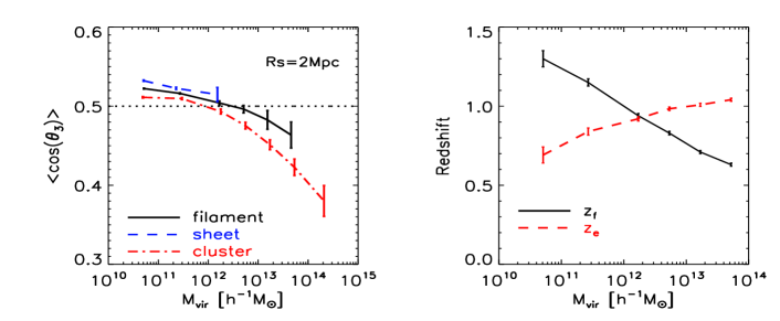
Figure 1: Left panel: The mean $\cos(\theta_{3})$ of halo spin-LSS as a function of halo mass at redshift $z=0$. Here $\theta_{3}$ is the angle between halo spin vector and the direction of large scale structure. Different color lines with error bars are for haloes in different environments at $z=0$. Right panel: The formation and entering time for haloes residing in filaments at $z=0$. The entering time is the redshift when the environment of the main progenitor of a $z=0$ halo changes from sheet to filament, see text for more detail.

3.1 Halo spin-LSS correlation in different environment

As a first step we show the halo spin -LSS correlation in different environment at $z=0$ in the left panel of Fig. 1. The blue dashed line for haloes in sheets, black solid for filaments, and red dash-dot line for cluster. In agreement with previous results (e.g., Hahn et al. 2007; Aragon-Calvo et al. 2007; Zhang et al. 2009), the halo spin in sheets are parallel to $\,{\bm{e_{3}}}$, and in filaments there is a mass dependence. The flip of spin-LSS occurs at haloes with mass around $3\times 10^{12}\,h^{-1}{\rm M}_{\odot}$, also agrees with other results (e.g., Codis et al. 2012). For the first time we show that in nodes, the spin of halo with mass $<5\times 10^{11}\,h^{-1}{\rm M}_{\odot}$ is align with $\,{\bm{e_{3}}}$, but turning into perpendicluar to $\,{\bm{e_{3}}}$ for more massive haloes. For haloes with mass bigger than flip mass, the alignment signal with more stronger mass dependence than in other environments.

The evolution of halo spin-LSS correlation from sheet to cluster environment can be understood as a consequence of cosmic web formation (e.g., Bond et al. 1996; Codis et al. 2012; Pichon et al. 2015): in sheet environment, the mass collaspe along the $\,{\bm{e_{1}}}$ direction is fastest (secondly along $\,{\bm{e_{2}}}$, slowest along $\,{\bm{e_{3}}}$), so mass flow is mostly from $\,{\bm{e_{1}}}$ and partly form $\,{\bm{e_{2}}}$ to the sheet plane ($\,{\bm{e_{2}}}$-$\,{\bm{e_{3}}}$ plane), and the resulted spin is in the sheet plane and being parallel to $\,{\bm{e_{3}}}$. With further collapse along $\,{\bm{e_{2}}}$, a filament begins to form, and the mass flow is mainly along $\,{\bm{e_{2}}}$ and the halo spin is still parallel to $\,{\bm{e_{3}}}$. At the final stage, when the mass along $\,{\bm{e_{3}}}$ is collapsed with formation of a node environment, the mass flow is mainly along $\,{\bm{e_{3}}}$ and the resulted spin is then being perpendicular to $\,{\bm{e_{3}}}$.

The above scenario is useful to understand the overall evolution of the spin-LSS correlation in different environments, but it is still not clear why in filament and cluster environment the spin of low-mass halo is parallel to filament, but being perpendicular to $\,{\bm{e_{3}}}$ for massive halo. It is obvious that in filament, the anisotropy of mass flow has a halo-mass dependence.

We mainly focus on the spin flip in filament in this $Letter$. It is naturally expected that this could be related to how long a halo has stayed in the filament. To investigate this, in the right panel of Fig. 1 we show the formation time and entering time for haloes in filaments at $z=0$. It is seen that the formation time of halo (black solid line) is mass dependent that low-mass halo forms first, in agreement with the CDM predictions (e.g., Navarro et al. 1997). But the red dashed line shows that low-mass haloes enter filaments later than larger haloes. Basically low-mass haloes enter filaments after they are formed ($z_{f}>z_{e}$), but high-mass haloes enter filaments before they are formed ($z_{e}>z_{f}$). The intersection between formation time and entering time occurs at halo with mass around $3\times 10^{12}\,h^{-1}{\rm M}_{\odot}$, very close the transit mass of spin-LSS relation in filament, and also close to the characteristic mass of collapsing halo at $z=0$.

3.2 The evolution of halo spin-LSS correlation

The right panel of Fig. 1 has important implication on the origin of the flip of halo spin-LSS correlation, it indicates that halo spin-LSS correlation could be linked to the time a halo has stayed in filament. To shed light on it, we divide haloes in filaments at $z=0$ into two sub-samples based on their virial mass, one is those with mass smaller than flip mass, $M_{flip}$, labeled as $align$ sample, the other is those with mass bigger than $M_{flip}$, labeled as $perp$ sample. Basically the $align$ sample are dominated by low-mass haloes and $perp$ sample are dominated by high-mass haloes.

In the left panel of Fig. 2 we show the time evolution of the spin-LSS correlation for the two sub-samples using solid and dashed lines. For each sub-sample, we plot the distribution of $\cos(\theta_{3})$ of their progenitors at the time of formation (blue lines), time of entering into filament (black lines). Remind that both the formation time $z_{f}$ and entering time $z_{e}$ of each halo is determined from its formation history. For comparison, we also plot the distribution of $\cos(\theta_{3})$ for the two sub-samples at $z=0$ with red lines.

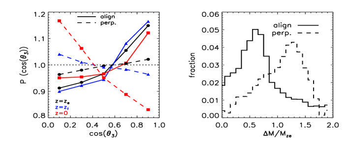
Figure 2: Left panel: The probability distribution of $\cos\theta_{3}$ at different redshifts for two sub-samples. Here we plot the spin-LSS correlation at three redshifts: $0$, $z_{e}$ (entering time) and $z_{f}$ (formation time). The value $P=1$ means a random distribution between halo spin vector and the direction of large scale structure, $\,{\bm{e_{3}}}$. Right panel: the distribution of mass growth rates for the two sub-samples, here $\Delta M=M_{0}-M_{z_{e}}$, in which $M_{z_{e}}$, $M_{0}$ is the virial mass of the progenitor halo at redshift $z=z_{e}$, and the mass of the descendant halo at $z=0$.

Fig. 2 shows an interesting evolution pattern. For the $align$ sample, the blue solid line shows that the times of their formation, their spin is parallel to the LSS, and when they enter the filament, their spin is still parallel to the filament, but becomes slightly weaker (black solid line). At $z=0$ their spin-filament alignment continuously become weaker, but still being align with filaments (red solid line). However, for the $perp$ sample, they enter filament firstly, with spin parallel to the filament (black dashed line). With mass grow in the filament, their spin becomes perpendicular to filament at time of formation (blue dashed line). At $z=0$ the mis-alignment signal becomes more stronger, and being perpendicular to the filaments (red dashed line).

In the right panel of Fig. 2 we show the mass growth for the two sub-samples of haloes. It is clearly seen that for $align$ haloes (solid line), their mass growth after entering filaments is lower and most haloes increase their mass by less than 80%. For $perp$ haloes (dashed line), their mass growth inside filament is significant, and most of them doubles their mass after entering the filament. Fig. 2 clear shows that for all haloes in filament at $z=0$, their initial spin is parallel to filament at the time when they enter filament, but the fate is different for low-mass and high-mass haloes. For low mass haloes, most of them mass is assembled before they enter into filament, although they accrete mass in filament environment, their spin is still parallel to the filament. For massive haloes, their mass growth inside filament is significant, so the mass accretion along filament led to their final spin to be perpendicular to filament.

4 Conclusion and Discussion

In this Letter, we investigate the origin of the mass dependence of halo spin with its environment. We find that there is an evolution pattern in the halo spin-LSS correlation in different large-scale environment that in sheets halo spin is parallel to LSS with almost no mass dependence. The halo spin-LSS correlation in filaments and nodes has a mass dependence that low-mass haloes have their spin being parallel to $\,{\bm{e_{3}}}$, and high-mass halo being perpendicular to $\,{\bm{e_{3}}}$. Such an evolution of halo spin-LSS correlation in different environment agrees with previous studies (e.g., Hahn et al. 2007; Codis et al. 2012).

We focus on the physical origin of halo spin in filament. We find that the mass dependence of halo spin-LSS is due to the mass dependence of halo formation time and halo migrating time from sheet to filament. For low-mass haloes, they forms first with spin being initially parallel to filament. After they enter into filament,their mass growth is minor, hardly changing their spin direction. For high-mass haloes, they firstly enter filament also with spin parallel to filament, but due to a significant mass growth inside filament, their final spin is perpendicular to filament. The scenario presented in this letter is in agreement with the scenario proposed by other studies (e.g., Codis et al. 2012; Welker et al. 2014; Pichon et al. 2015). Our explanation is more general by connecting halo formation and migrating time which can be further tested using observational data. In addition, we also find the the conclusion still holds for haloes in cluster region. For more detals, we will discuss in our next paper.

Although observational test of simulated prediction of halo spin with the large scale environment is not easy, recent progress using large sky survey make it possible, such as those studies by a few authors (e.g., Zhang et al. 2014). In particular, Tempel & Libeskind (2013) confirmed the mass dependence of galaxy spin with large scale structure using local observations. Our results suggests the halo spin-LSS is evolving, depending on halo formation time and mass accretion history, it is thus expected that such a correlation is dependent on galaxy properties, such as color, star formation rate, and the correlation will also evolve with redshift. With more survey data available at high redshifts in future, the predicted galaxy spin-LSS can be further tested, as achieved by a recent work using VIMOS survey (Malavasi et al. 2016).

On the other hand, our results in this paper are based on CDM simulation, and it is well know that dark matter halo forms hierarchically in CDM and the environment changes subsequently from sheet to filament and to node finally. Current results and proposed scenario support the CDM model. However, if the dark matter mass is not cold, such as hot or warm dark matter, the formation of dark matter halo and its relation to environment will proceed in a different way (e.g., Colombi et al. 1996; Knebe et al. 2003; Bode et al. 2001; Frenk & White 2012). In that case our scenario of halo spin-LSS correlation will predict a different correlation and evolution. More studies can be done using N-body simulations to investigate the predictions in other models of dark matter particle or structure formation scenario.

5 Acknowledgments

The work is supported by the 973 program (No. 2015CB857003, No. 2013CB834900), NSF of Jiangsu Province (No. BK20140050), the NSFC (No. 11333008) and the Strategic Priority Research Program the emergence of cosmological structures of the CAS (No. XDB09010403). The simulations are run on the supercomputing center of PMO.

References

- Aragón-Calvo et al. (2007) Aragón-Calvo M. A., Jones B. J. T., van de Weygaert R., van der Hulst J. M., 2007, A&A, 474, 315
- Aragón-Calvo et al. (2007) Aragón-Calvo M. A., van de Weygaert R., Jones B. J. T., van der Hulst J. M., 2007, ApJ, 655, L5
- Aragon-Calvo & Yang (2014) Aragon-Calvo M. A., Yang L. F., 2014, MNRAS, 440, L46
- Bode, Ostriker, & Turok (2001) Bode P., Ostriker J. P., Turok N., 2001, ApJ, 556, 93
- Bond, Kofman, & Pogosyan (1996) Bond J. R., Kofman L., Pogosyan D., 1996, Natur, 380, 603
- Cautun et al. (2014) Cautun M., van de Weygaert R., Jones B. J. T., Frenk C. S., 2014, MNRAS, 441, 2923
- Codis et al. (2012) Codis S., Pichon C., Devriendt J., Slyz A., Pogosyan D., Dubois Y., Sousbie T., 2012, MNRAS, 427, 3320
- Colombi, Dodelson, & Widrow (1996) Colombi S., Dodelson S., Widrow L. M., 1996, ApJ, 458, 1
- Davis et al. (1985) Davis M., Efstathiou G., Frenk C. S., White S. D. M., 1985, ApJ, 292, 371
- Forero-Romero, Contreras, & Padilla (2014) Forero-Romero J. E., Contreras S., Padilla N., 2014, MNRAS, 443, 1090
- Frenk & White (2012) Frenk C. S., White S. D. M., 2012, AnP, 524, 507
- Hahn et al. (2007) Hahn O., Carollo C. M., Porciani C., Dekel A., 2007, MNRAS, 381, 41
- Hahn et al. (2007) Hahn O., Porciani C., Carollo C. M., Dekel A., 2007, MNRAS, 375, 489
- Joachimi et al. (2015) Joachimi B., et al., 2015, SSRv, 193, 1
- Jones, van de Weygaert, & Aragón-Calvo (2010) Jones B. J. T., van de Weygaert R., Aragón-Calvo M. A., 2010, MNRAS, 408, 897
- Kang et al. (2005) Kang X., Jing Y. P., Mo H. J., Börner G., 2005, ApJ, 631, 21
- Kang & Wang (2015) Kang X., Wang P., 2015, ApJ, 813, 6
- Knebe et al. (2003) Knebe A., Devriendt J. E. G., Gibson B. K., Silk J., 2003, MNRAS, 345, 1285
- Komatsu et al. (2011) Komatsu E., et al., 2011, ApJS, 192, 18
- Laigle et al. (2015) Laigle C., et al., 2015, MNRAS, 446, 2744
- Lee & Pen (2002) Lee J., Pen U.-L., 2002, ApJ, 567, L111
- Libeskind et al. (2013) Libeskind N. I., Hoffman Y., Steinmetz M., Gottlöber S., Knebe A., Hess S., 2013, ApJ, 766, L15
- Libeskind et al. (2014) Libeskind N. I., Knebe A., Hoffman Y., Gottlöber S., 2014, MNRAS, 443, 1274
- Malavasi et al. (2016) Malavasi N., et al., 2016, arXiv, arXiv:1611.07045
- Navarro, Frenk, & White (1997) Navarro J. F., Frenk C. S., White S. D. M., 1997, ApJ, 490, 493
- Peebles (1969) Peebles P. J. E., 1969, ApJ, 155, 393
- Pichon et al. (2011) Pichon C., Pogosyan D., Kimm T., Slyz A., Devriendt J., Dubois Y., 2011, MNRAS, 418, 2493
- Pichon et al. (2014) Pichon C., Codis S., Pogosyan D., Dubois Y., Desjacques V., Devriendt J., 2014, arXiv, arXiv:1409.2608
- Porciani, Dekel, & Hoffman (2002) Porciani C., Dekel A., Hoffman Y., 2002, MNRAS, 332, 325
- Sheth & Tormen (2004) Sheth R. K., Tormen G., 2004, MNRAS, 349, 1464
- Shi, Wang, & Mo (2015) Shi J., Wang H., Mo H. J., 2015, ApJ, 807, 37
- Sousbie et al. (2008) Sousbie T., Pichon C., Colombi S., Novikov D., Pogosyan D., 2008, MNRAS, 383, 1655
- Springel (2005) Springel V., 2005, MNRAS, 364, 1105
- Tempel & Libeskind (2013) Tempel E., Libeskind N. I., 2013, ApJ, 775, L42
- Trowland, Lewis, & Bland-Hawthorn (2013) Trowland H. E., Lewis G. F., Bland-Hawthorn J., 2013, ApJ, 762, 72
- Trujillo et al. (2006) Trujillo I., Carretero C., Patiri S., 2006, ApjL, 640, 111
- van de Weygaert et al. (2016) van de Weygaert R., Shandarin S., Saar E., Einasto J., 2016, IAUS, 308,
- van Haarlem & van de Weygaert (1993) van Haarlem M., van de Weygaert R., 1993, ApJ, 418, 544
- Wang et al. (2005) Wang H. Y., Jing Y. P., Mao S., Kang X., 2005, MNRAS, 364, 424
- Wang et al. (2014) Wang Y. O., Lin W. P., Kang X., Dutton A., Yu Y., Macciò A. V., 2014, ApJ, 786, 8
- Welker et al. (2014) Welker C., Devriendt J., Dubois Y., Pichon C., Peirani S., 2014, MNRAS, 445, L46
- White (1984) White S. D. M., 1984, ApJ, 286, 38
- Zel’dovich (1970) Zel’dovich Y. B., 1970, A&A, 5, 84
- Zhang et al. (2009) Zhang Y., Yang X., Faltenbacher A., Springel V., Lin W., Wang H., 2009, ApJ, 706, 747
- Zhang et al. (2015) Zhang Y., Yang X., Wang H., Wang L., Luo W., Mo H. J., van den Bosch F. C., 2015, ApJ, 798, 17