A scattering-based algorithm for wave propagation in one dimension

Abstract

We present an explicit numerical scheme to solve the variable coefficient wave equation in one space dimension with minimal restrictions on the coefficient and initial data.

MSC 35L05, 65M; Keywords: one dimensional wave equation, numerical methods, scattering

1 The algorithm

A range of physical and biological applications involve the one dimensional wave equation

$$u_{tt}-\textstyle\frac{1}{\zeta}(\zeta u_{x})_{x}=0$$ (1.1a)

$$u(x,0)=f(x),\qquad u_{t}(x,0)=g(x)$$ (1.1b)

where: there exist $x_{-}<x_{+}$ such that $\zeta$ takes constant values $\zeta_{-}$ and $\zeta_{+}$ on the respective intervals $(-\infty,x_{-})$ and $(x_{+},\infty)$; and $0<c<\zeta<C$ for some $c<C\in\mathbb{R}$. Applications include imaging of layered media such as seismic imaging and the acoustic imaging of laminated structures, microwave imaging of skin tissue, and modelling the human vocal tract and cochlea; see [8],[3], [17], [16], [18]. Certain of these applications have a long history, yet there seems to be no clear consensus on how best to compute solutions to (1.1) in the general setting where $\zeta$ has complicated structure on $[x_{-},x_{+}]$ such as rapid oscillations or discontinuities, or where the initial data is singular (e.g., a Dirac comb), or both (for background see [14, Ch. 10], [1, Ch. 5], [12, Ch. 9]). Recent theoretical insights into the case where $\zeta$ is piecewise constant offer a fresh perspective from which to consider the numerical analysis of (1.1) for general $\zeta$ ([9], [10]).

The purpose of this note is to present a simple, explicit numerical scheme to solve (1.1) on a region $(x,t)\in[a,b]\times[0,T]\subset\mathbb{R}^{2}$ where $[x_{-},x_{+}]\subset[a,b]$. The scheme is based on a natural idea from scattering theory, but with crucial differences from established methods in both the details of the implementation and the interpretation. These differences yield an order of magnitude reduction in computational expense coupled with remarkable versatility.

Algorithm 1.

Preliminary step. Convert the initial data $f(x)$ and $g(x)$ from (1.1b) to a pair of functions

$$\alpha(x)=\frac{1}{2}\left(f(x)-\frac{1}{\zeta(x)}\int_{-\infty}^{x}\zeta(s)g(s)\,ds\right),\;\beta(x)=\frac{1}{2}\left(f(x)+\frac{1}{\zeta(x)}\int_{-\infty}^{x}\zeta(s)g(s)\,ds\right).$$ (1.2)

The scattering algorithm
Input	$\zeta,\alpha,\beta,a,b,n,T$
Spatial grid	$\Delta=(b-a)/n,\quad x_{j}=a+(j-1)\Delta\qquad(1\leq j\leq n+1)$
Temporal grid	$m=\lfloor T/\Delta\rfloor,\quad t_{k}=k\Delta\qquad(0\leq k\leq m)$
Weights	$r_{j}=\bigl{(}\zeta(x_{j})-\zeta(x_{j+1})\bigr{)}/\bigl{(}\zeta(x_{j})+\zeta(x_{j+1})\bigr{)}\qquad(1\leq j\leq n)$
Variables	$v=\bigl{(}v^{k}_{i}\bigr{)}\in\mathbb{R}^{(m+1)\times(2n+2)},\quad\tilde{u}=\bigl{(}\tilde{u}^{k}_{j}\bigr{)}\in\mathbb{R}^{(m+1)\times(n+1)}$
Initialization	$v^{0}_{2j-1}=\alpha(x_{j}),\quad v^{0}_{2j}=\beta(x_{j}),\quad\tilde{u}^{0}_{j}=v^{0}_{2j-1}+v^{0}_{2j}\qquad(1\leq j\leq n+1)$
	$v^{k}_{1}=\alpha(x_{1}-t_{k}),\quad v^{k}_{2n+2}=\beta(x_{n+1}+t_{k})\qquad(1\leq k\leq m)$
Iterative step	Given $v^{k}$ $(0\leq k\leq m-1)$, set
	$v^{k+1}_{2j-1}=(1+r_{j-1})v^{k}_{2j-3}-r_{j-1}v^{k}_{2j}\qquad(2\leq j\leq n+1)$
	$v^{k+1}_{2j}=r_{j}v^{k}_{2j-1}+(1-r_{j})v^{k}_{2j+2}\qquad(1\leq j\leq n)$
	$\tilde{u}^{k+1}_{j}=v^{k+1}_{2j-1}+v^{k+1}_{2j}\qquad(1\leq j\leq n+1)$
Output	$\tilde{u}=\bigl{(}\tilde{u}^{k}_{j}\bigr{)}\in\mathbb{R}^{(m+1)\times(n+1)}$

2 Discussion

Rather than discretize derivatives, the idea behind Algorithm 1 is to replace $\zeta$ with a step function and solve the resulting equation exactly. This echoes the piecewise constant approximations of Goupillaud and Godunov and their many subsequent manifestations (cf. [2], [11], [5], [7], [8, Ch. 3]); however, Algorithm 1 differs markedly from previously established methods. In detail, let $x_{j}^{\ast}=(x_{j}+x_{j+1})/2$ $(1\leq j\leq n)$ denote the midpoints of consecutive spatial grid points, write $P=\{x_{1},x_{1}^{\ast},x_{2},x_{2}^{\ast},\ldots,x_{n},x_{n}^{\ast},x_{n+1}\},$ and set

$$\zeta^{P}(x)=\left\{\begin{array}[]{ll}\zeta_{-}&\mbox{ if }x<x_{1}^{\ast}\\ \zeta(x_{j})&\mbox{ if }x_{j-1}^{\ast}\leq x<x_{j}^{\ast}\quad(2\leq j\leq n)\\ \zeta_{+}&\mbox{ if }x_{n}^{\ast}\leq x\end{array}\right..$$ (2.1)

Then $\zeta^{P}$ is a step function having equally spaced jump points $x_{1}^{\ast},\ldots,x_{n}^{\ast}$, and it coincides with $\zeta$ on the spatial grid. Replacing $\zeta$ by $\zeta^{P}$ in (1.1) yields

$$u_{tt}-\textstyle\frac{1}{\zeta^{P}}(\zeta^{P}u_{x})_{x}=0$$ (2.2a)

$$u(x,0)=f(x),\qquad u_{t}(x,0)=g(x),$$ (2.2b)

the first equation of which reduces to $u_{tt}-u_{xx}=0$ on intervals of the form $(-\infty,x_{1}^{\ast})$, $(x_{j-1}^{\ast},x_{j}^{\ast})$ or $(x_{n}^{\ast},\infty)$, where $\zeta^{P}$ is constant. Its solution within each such interval is therefore a pair of left and right travelling waves. One-sided limits of $u$ and $\zeta^{P}u_{x}$ are required to agree at each jump point $x_{j}^{\ast}$

$$u(x_{j}^{\ast}-,t)=u(x_{j}^{\ast}+,t)\quad\mbox{ and }\quad\zeta^{P}(x_{j})u_{x}(x_{j}^{\ast}-,t)=\zeta^{P}(x_{j+1})u_{x}(x_{j}^{\ast}+,t).$$

By a standard computation (see [8, Ch. 3]), this yields reflection and transmission factors: a right-travelling wave in $(x_{j-1}^{\ast},x_{j}^{\ast})$ gets partially reflected back off $x_{j}^{\ast}$, with reflection factor $r_{j}$ as defined in Algorithm 1, and partially transmitted into $(x_{j}^{\ast},x_{j+1}^{\ast})$, with transmission factor $1+r_{j}$. In particular, characteristic lines for the equation (2.2a) bifurcate at jump points of $\zeta^{P}$. The corresponding domains of dependence and influence for a grid point $(x_{j},t_{k})$ are depicted in Figure 1. In Algorithm 1 the pair $v^{k}_{2j-1},v^{k}_{2j}$ encodes the respective amplitudes of the right and left moving parts of the solution to (2.2) at the grid point $(x_{j},t_{k})$, and the iterative step accounts for the reweighted reflected and transmitted waves comprising the domain of dependence of $(x_{j},t_{k+1})$ at time $t_{k}$. In this way the algorithm computes the exact solution to (2.2) at the grid points.

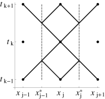
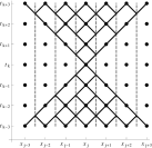
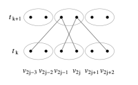
Figure 1: Forward and backward characteristics through a grid point $(x_{j},t_{k})$ in the presence of discontinuities. Left: one time step, center: several time steps. Right: the stencil for Algorithm 1 with respect to the values $v^{k}_{i}$, pairs of which correspond to spatial grid points.

The matrix formulation of the dependence of (row vector) $v^{k+1}$ on $v^{k}$ as expressed in the scattering algorithm is

$$v^{k+1}=v^{k}A_{P}+(v^{k+1}_{1},0,\ldots,0,v^{k+1}_{2n+2}),$$ (2.3)

where $A_{P}$ is a $(2n+2)\times(2n+2)$ pentadiagonal matrix having $4n$ non-zero entries. For example, if $n=4$,

$$A_{P}=\left(\begin{array}[]{cccccccccc}0&r_{1}&r_{1}+1&0&0&0&0&0&0&0\\ 0&0&0&0&0&0&0&0&0&0\\ 0&0&0&r_{2}&r_{2}+1&0&0&0&0&0\\ 0&1-r_{1}&-r_{1}&0&0&0&0&0&0&0\\ 0&0&0&0&0&r_{3}&r_{3}+1&0&0&0\\ 0&0&0&1-r_{2}&-r_{2}&0&0&0&0&0\\ 0&0&0&0&0&0&0&r_{4}&r_{4}+1&0\\ 0&0&0&0&0&1-r_{3}&-r_{3}&0&0&0\\ 0&0&0&0&0&0&0&0&0&0\\ 0&0&0&0&0&0&0&1-r_{4}&-r_{4}&0\end{array}\right).$$ (2.4)

Solutions to (2.2) outlined in, e.g., [5] and [8] involve upper or lower triangular systems requiring approximately $Tn^{3}/(b-a)$ flops, while the sparse structure of $A_{P}$ reduces this to $7Tn^{2}/(b-a)$ flops. Thus Algorithm 1 is qualitatively faster than previously established methods, allowing computation on a vastly finer spatial grid.

The following facts justify Algorithm 1 theoretically.

Theorem 1.

The eigenvalues of $A_{P}$ lie properly inside the unit circle, implying stability of the scattering algorithm.

Proof.   Let $U_{P}$ denote the $(2n+2)\times(2n+2)$ pentadiagonal matrix

$$\begin{split}&U_{P}=\\ &\left(\begin{array}[]{cccccccccc}0&r_{1}&\sqrt{1-r_{1}^{2}}&&&&&&&\\ 1&0&0&0&&&&&\mbox{\Large$0$}&\\ 0&0&0&r_{2}&\sqrt{1-r_{2}^{2}}&&&&&\\ &\sqrt{1-r_{1}^{2}}&-r_{1}&0&0&0&&&&\\ &&0&0&0&\ddots&\ddots&&&\\ &&&\sqrt{1-r_{2}^{2}}&-r_{2}&\ddots&0&0&&\\ &&&&\ddots&\ddots&0&r_{n}&\sqrt{1-r_{n}^{2}}&\\ &&&&&\sqrt{1-r_{n-1}^{2}}&-r_{n-1}&0&0&0\\ &\mbox{\Large$0$}&&&&&0&0&0&1\\ &&&&&&&\sqrt{1-r_{n}^{2}}&-r_{n}&0\end{array}\right).\end{split}$$ (2.5)

$U_{P}$ is evidently unitary since its columns (and rows) are pairwise orthogonal. Set

$$\sigma_{j}=\prod_{k=j}^{n}\sqrt{\frac{1+r_{k}}{1-r_{k}}}=\sqrt{\frac{\zeta(x_{j})}{\zeta(x_{n+1})}}\qquad(1\leq j\leq n),$$

and let $D_{P}$ denote the $(2n+2)\times(2n+2)$ diagonal matrix

$$D_{P}=\operatorname{diag}(\sigma_{1},\sigma_{1},\sigma_{2},\sigma_{2},\ldots,\sigma_{n},\sigma_{n},1,1).$$ (2.6)

Let $J$ denote the $(2n+2)\times(2n+2)$ diagonal projection of rank $2n$ obtained by zeroing out the first and last diagonal entries of the identity matrix,

$$J=\operatorname{diag}(0,1,1,\ldots,1,0).$$

Then by direct computation,

$$A_{P}=D_{P}(U_{P}J)D_{P}^{-1}.$$

Thus the spectrum of $A_{P}$ is the same as that of $U_{P}J$. Note that for any column vector $v$, $\lVert Jv\rVert\leq\lVert v\rVert$, with equality only if $Jv=v$. If $U_{P}Jv=\lambda v$ for some scalar $\lambda$, then, since $U_{P}$ is unitary,

$$|\lambda|\lVert v\rVert=\lVert U_{P}Jv\rVert=\lVert Jv\rVert\leq\lVert v\rVert.$$

Hence the spectrum of $U_{P}J$ belongs to the closed unit disk. If $|\lambda|=1$, then $Jv=v$, as noted above, and hence $U_{P}v=\lambda v$. Given that $|\lambda|=1$, this forces $v=0$, as follows. Note that $v_{1}=v_{2n+2}=0$ since $Jv=v$. Since $U_{P}v=\lambda v$, the structure of the second row of $U_{P}$ in (2.5) implies that $v_{1}=\lambda v_{2}$, so $v_{2}=0$. Looking at the first row of (2.5), $r_{1}v_{2}+\sqrt{1-r_{1}^{2}}v_{3}=\lambda v_{1}$, forcing $v_{3}=0$. In general, if $v_{2k}=v_{2k+1}=0$ for some $1\leq k\leq n-1$, then inspection of row $2k+2$ of $U_{P}$, followed by $2k+1$ yields that $v_{2k+2}=v_{2k+3}=0$. Since $v_{2n+2}=0$ this proves $v=0$ as claimed. Thus if $|\lambda|=1$ then $\lambda$ is not an eigenvalue, so the spectrum of $U_{P}J$ and hence that of $A_{P}$, is contained in the interior of the unit disk.  

Theorem 2.

Let $u^{P}$ denote the solution to (2.2), $(x_{j},t_{k})$ an arbitrary grid point as defined in Algorithm 1, and $\tilde{u}$ the output of the algorithm.

1. If $\alpha$ and $\beta$ are regular functions (as opposed to distributions), then $u^{P}(x_{j},t_{k})=\tilde{u}^{k}_{j}$.

2. If $\alpha(x)=\sum_{j\in\mathbb{Z}}c_{j}\delta(x-a-j\Delta)$ and $\beta(x)=\sum_{j\in\mathbb{Z}}d_{j}\delta(x-a-j\Delta)$ are Dirac combs supported on an extension of the spatial grid, and values of $\alpha$ and $\beta$ are replaced in Algorithm 1 by the corresponding coefficients $c_{j}$ and $d_{j}$, then $u^{P}(x_{j},t_{k})=\tilde{u}^{k}_{j}\;\delta(x-a-j\Delta)$.

Proof.   Let $\alpha_{k}$ and $\beta_{k}$ denote the respective right and left-moving components of $u^{P}$ at time $t_{k}$ analogous to (1.2),

$$\begin{split}\alpha_{k}(x)&=\frac{1}{2}\left(u^{P}(x,t_{k})-\frac{1}{\zeta(x)}\int_{-\infty}^{x}\zeta(s)u^{P}_{t}(s,t_{k})\,ds\right)\mbox{ and }\\ \beta_{k}(x)&=\frac{1}{2}\left(u^{P}(x,t_{k})+\frac{1}{\zeta(x)}\int_{-\infty}^{x}\zeta(s)u^{P}_{t}(s,t_{k})\,ds\right).\end{split}$$

The standard laws of reflection and transmission described above imply that for $x\in(x_{j-1}^{\ast},x_{j}^{\ast})$,

$$\begin{split}\alpha_{k+1}(x)&=(1+r_{j-1})\alpha_{k}(x-\Delta)-r_{j-1}\beta_{k}(x_{j}^{\ast}-(x-x_{j-1}^{\ast}))\quad\mbox{ and }\\ \beta_{k+1}(x)&=r_{j}\alpha_{k}(x_{j}^{\ast}-(x-x_{j-1}^{\ast}))+(1-r_{j})\beta_{k}(x+\Delta).\end{split}$$

See Figure 1. These formulas can be given a valid interpretation for distributions (evaluated on appropriately chosen test functions) as well as ordinary functions. Specializing to the point $x=x_{j}\in(x_{j-1}^{\ast},x_{j}^{\ast})$ yields the formulas

$$\alpha_{k+1}(x_{j}) =(1+r_{j-1})\alpha_{k}(x_{j-1})-r_{j-1}\beta_{k}(x_{j})\quad\mbox{ and }$$ (2.7a)

$$\beta_{k+1}(x_{j}) =r_{j}\alpha_{k}(x_{j})+(1-r_{j})\beta_{k}(x+\Delta).$$ (2.7b)

The latter formulas make sense for ordinary functions $\alpha_{k},\beta_{k}$. But distributions do not in general have meaningful restrictions to a single point—unless they are supported at a single point, such as is the case for Dirac functions. Thus formulas (2.7), which are precisely the iterative step of the scattering algorithm, apply both to ordinary functions and Dirac distributions, proving that the algorithm coincides with the exact solution to (1.1) in these cases.  

Theorem 3.

If there is a sequence of partitions $\{P\}$ such that $\zeta^{P}\rightarrow\zeta$ uniformly, then $u^{P}\rightarrow u$ on $[a,b]\times[0,T]$ in an appropriate sense depending on the smoothness of the initial data.

The convergence $u^{P}\rightarrow u$ is uniform if initial data are smooth; for certain distributional initial data the convergence may be in the Sobolev space $H^{-1}$. Proofs and full technical details will be presented elsewhere. In essence, Theorem 3 follows from abstract functional analysis such as [15, Ch. 3.8] or [4, Ch. 10]. See [13, Theorem 3.5] for a particular version, proved by way of the Hille-Yosida theorem. The heuristic upshot of Theorem 3 is that uniform convergence of the coefficient $u^{P}$ drives convergence of the solution.

Combining Theorems 2 and 3 one can exploit a separation of scales phenomenon to compute both the regular and singular parts of the solution $u(x,t)$ to (1.1) in the case of Dirac function initial data. The solutions to the approximations $u^{P}$ are Dirac combs whose components have the form $\gamma\delta(x-x_{j}-t_{k})$. If $(x_{j},t_{k})$ is a common grid point for a succession of partitions $P$, then the rescaled coefficient $\gamma/\Delta$ diverges if $(x_{j},t_{k})$ belongs to the singular support of $u$; otherwise $\gamma/\Delta$ converges to the regular value of $u(x_{j},t_{k})$. On the other hand, the unscaled coefficient $\gamma$ goes to zero at regular points and stabilizes at singular points. See Figure 2.

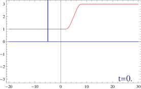
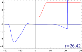
Figure 2: Computation of a Dirac impulse (plotted as a blue vertical half line) traversing a smooth ramp $\zeta$, depicted in red. Left: an initially right moving unit pulse at left of the ramp. Middle: after the pulse has traversed the ramp, a smooth reflected waveform travels to the left and a mixed waveform, consisting of a Dirac pulse followed by a regular function, travels to the right. In order to match the scale of the ramp, the amplitude of the waveforms has been scaled up by a factor of 32. Right: a log-log plot of relative rms error $E(n)$ of the plotted waveform for $n=2^{p}$, $p=7,8,9,10,11,12,13$. The slope is very close to $-1$, corresponding to $E(n)\cong 7.4/n$. Computation time is 6 seconds for $p=10$, at which point the plot is indistinguishable from that of the exact result.

Algorithm 1 also handles the contrasting scenario in which initial data is smooth and $\zeta$ is a highly oscillatory step function. If the jump points of $\zeta$ are equally spaced, one can choose $P$ such that $\zeta^{P}=\zeta$, whereby the algorithm is exact up to roundoff error (by Theorem 2). Comparison with the (much slower) exact methods of [9] shows that a good approximation is also obtained if the jump points of $\zeta$ are not equally spaced, provided the underlying grid is sufficiently fine. Indeed, Algorithm 1 reveals a remarkable qualitative phenomenon whereby smooth initial data can lead to discontinuities, as illustrated in Figure 3.

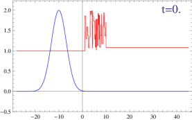
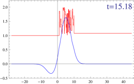
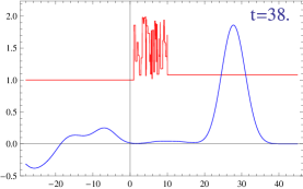
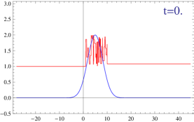
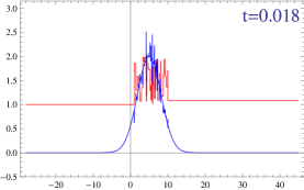
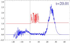
Figure 3: The case where $\zeta$, depicted in red, is a highly oscillatory step function. Top row: an initially smooth wave form (plotted in blue) traverses the oscillatory zone from left to right, resulting in continuous transmitted and reflected wave forms. Bottom row: a smooth, right-travelling wave form initially within the oscillatory region spontaneously forms discontinuities, which persist in the resulting right and left-moving wave forms. This surprising phenomenon may be verified analytically, the simplest case being where $\zeta$ has just a single jump point.

The gist of Theorems 1, 2 and 3 is that Algorithm 1 is guaranteed to approximate the solution to the original equation (1.1) in a wide range of cases, including with distributional initial data. Up to roundoff error, the approximation is exact for piecewise constant $\zeta$, provided its jump points are included in those of $\zeta^{P}$, irrespective of whether the initial data are smooth or singular. The general requirement that $\zeta$ be a uniform limit of step functions (i.e., a regulated function) is very weak, allowing $\zeta$ to have essentially arbitrary structure on $[x_{-},x_{+}]$ (see [6, Ch. VII]). Thus Algorithm 1 differs essentially from existing methods in its interpretation—initial data may be non-smooth or purely distributional, and the coefficient $\zeta$ may have discontinuities.

It does not appear that Algorithm 1 can be generalized to higher dimensions in a way that retains the exactness results of Theorem 2—in this sense the method is purely one dimensional. Within the context of one-dimensional evolutionary systems governed by (1.1) however, the algorithm marks a qualitative improvement over existing methods in terms of both speed and generality. In summary, Algorithm 1 comprises an easily-implemented, versatile and accurate computational tool applicable to various imaging modalities and to modelling of various biological or built structures.

Appendix A Computational data

The present section gives further details on Figures 2 and 3 to facilitate replication of the results. The smooth ramp in Figure 2 is given by the formula

$$\zeta(x)=\left\{\begin{array}[]{cc}1&\mbox{ if }x\leq 1\\ \rule[-10.0pt]{0.0pt}{28.0pt}2+\tanh\left(\frac{8(x-5)}{16-(x-5)^{2}}\right)&\mbox{ if }1<x<9\\ 3&\mbox{ if }9\leq x\end{array}\right..$$

The source is a right moving unit Dirac function initially centered at $x=-5$.

In the case of Figure 3, $\zeta$ is a step function with 40 randomly generated jump points lying in the interval $[1,10]$. $\zeta(x)=1$ for $x<1$ and $\zeta(x)=2/3$ for $x>10$. The source wave is a right-travelling gaussian initially of the form

$$\alpha(x)=2e^{-.05(x+10)^{2}}$$

in the first example; the source is shifted 15 units to the right in the second example. The qualitative nature of the propagating wavefield does not depend on the detailed structure of the step function.

References

• [1] U. M. Ascher. Numerical methods for evolutionary differential equations, volume 5 of Computational Science & Engineering. Society for Industrial and Applied Mathematics (SIAM), Philadelphia, PA, 2008.
• [2] L. H. Berryman, P. L. Goupillaud, and K. H. Waters. Reflections from multiple transition layers part I—theoretical results. Geophysics, 23(2):223–243, 1958.
• [3] N. Bleistein, J. K. Cohen, and J. W. Stockwell, Jr. Mathematics of multidimensional seismic imaging, migration, and inversion, volume 13 of Interdisciplinary Applied Mathematics. Springer-Verlag, New York, 2001. Geophysics and Planetary Sciences.
• [4] H. Brezis. Functional analysis, Sobolev spaces and partial differential equations. Universitext. Springer, New York, 2011.
• [5] K. P. Bube and R. Burridge. The one-dimensional inverse problem of reflection seismology. SIAM Rev., 25(4):497–559, 1983.
• [6] J. Dieudonné. Foundations of modern analysis. Pure and Applied Mathematics, Vol. X. Academic Press, New York-London, 1960.
• [7] T. R. Fogarty and R. J. LeVeque. High-resolution finite-volume methods for acoustic waves in periodic and random media. The Journal of the Acoustical Society of America, 106(1), 1999.
• [8] J.-P. Fouque, J. Garnier, G. Papanicolaou, and K. Sølna. Wave propagation and time reversal in randomly layered media, volume 56 of Stochastic Modelling and Applied Probability. Springer, New York, 2007.
• [9] P. C. Gibson. The combinatorics of scattering in layered media. SIAM J. Appl. Math., 74(4):919–938, 2014.
• [10] P. C. Gibson. Fourier expansion of disk automorphisms via scattering in layered media. Journal of Fourier Analysis and Applications, pages 1–22, 2016.
• [11] S. K. Godunov. A difference method for the calculation of shock waves. Amer. Math. Soc. Transl. (2), 16:389–390, 1960.
• [12] B. Gustafsson. High order difference methods for time dependent PDE, volume 38 of Springer Series in Computational Mathematics. Springer-Verlag, Berlin, 2008.
• [13] A. Kirsch and A. Rieder. Inverse problems for abstract evolution equations with applications in electrodynamics and elasticity. Inverse Problems, 32(08):085001, 24, 2016.
• [14] R. J. LeVeque. Finite difference methods for ordinary and partial differential equations. Society for Industrial and Applied Mathematics (SIAM), Philadelphia, PA, 2007. Steady-state and time-dependent problems.
• [15] J.-L. Lions and E. Magenes. Non-homogeneous boundary value problems and applications. Vol. I. Springer-Verlag, New York-Heidelberg, 1972. Translated from the French by P. Kenneth, Die Grundlehren der mathematischen Wissenschaften, Band 181.
• [16] K. van den Doel and U. M. Ascher. Real-time numerical solution of webster’s equation on a nonuniform grid. IEEE Transactions on Audio, Speech, and Language Processing, 16(6):1163–1172, Aug 2008.
• [17] T. Williams, E. Fear, and D. Westwick. Tissue sensing adaptive radar for breast cancer detection-investigations of an improved skin-sensing method. Microwave Theory and Techniques, IEEE Transactions on, 54(4):1308 – 1314, june 2006.
• [18] G. Zweig and C. A. Shera. The origin of periodicity in the spectrum of evoked otoacoustic emissions. The Journal of the Acoustical Society of America, 98(4):2018–2047, 1995.