Numerical simulation of polynomial-speed convergence phenomenon

Abstract.

We provide a hybrid method that captures the polynomial speed of convergence and polynomial speed of mixing for Markov processes. The hybrid method that we introduce is based on the coupling technique and renewal theory. We propose to replace some estimates in classical results about the ergodicity of Markov processes by numerical simulations when the corresponding analytical proof is difficult. After that, all remaining conclusions can be derived from rigorous analysis. Then we apply our results to seek numerical justification for the ergodicity of two 1D microscopic heat conduction models. The mixing rate of these two models are expected to be polynomial but very difficult to prove. In both examples, our numerical results match the expected polynomial mixing rate well.

1. Introduction

The aim of this paper is two-fold. From the viewpoint of statistical mechanics, this paper aims to justify the polynomial ergodicity of a class of 1D microscopic heat conduction models. Purely rigorous analysis of polynomial ergodicity of these models using current analytical techniques fails to provide satisfactorily accurate results. This paper also aims to establish a comprehensive method that can be applied on a broader scale. That is, from the viewpoint of numerical analysis, we also want to propose a hybrid method that captures polynomial-speed convergence to steady-states for general Markov processes.

Heat conduction is ubiquitous in the universe and has been well-studied at the macroscopic level. However, from a microscopic point of view, the study of how energy is transported in materials is a very challenging topic. In particular, the derivation of Fourier’s law from microscopic Hamiltonian dynamics is a century-old challenge to mathematicians and physicists [4, 13, 14, 16, 43, 5]. Due to the significant difficulty of analyzing Hamiltonian models, many researchers seek stochastic approximations of Hamiltonian dynamics in microscopic heat conduction models [14, 31, 16, 28, 17, 11]. In this paper, we will work primarily on these stochastic heat conduction models.

When an 1D stochastic heat conduction model is connected to two thermalized boundaries with different temperatures, one would expect the existence of a naturally selected steady-state, called the non-equilibrium steady-state (NESS). An analysis of topics like existence and uniqueness of NESS, and speed of convergence to NESS will open the door to further studies such as the thermal conductivity, the existence of local thermodynamic equilibrium, the Gallavotti-Cohen fluctuation theorem, and eventually the Fourier’s law. However, a rigorous analysis about the ergodicity of the NESS is usually very challenging.

Due to complicated interactions within the chain, a stochastic microscopic heat conduction model may have sub-exponential speed of mixing and sub-exponential speed of convergence to the NESS. In this paper we will present two 1D microscopic heat conduction models, namely, the stochastic energy exchange model and the random halves model, both of which originate from deterministic dynamical systems [14, 6, 31]. One common feature of these two models is that a low energy particle (or a low energy site) requires a long time to have the next energy exchange. Because of this, we expect the rate of convergence and the rate of mixing to be $\sim t^{-2}$. We refer readers to Section 5 and Section 6 for more engaged discussion about microscopic heat conduction models and their connections to deterministic dynamical systems. Besides these two models, other microscopic heat conduction models that have sub-exponential mixing rate include the particle model in [50, 49], the rotor model in [9, 10], and the anharmonic chain in [21]. Other examples of sub-exponential rate of convergence have also been observed in various models like MCMC algorithms and random walks [26, 47, 36].

Regardless of the detailed setting of models, a rigorous proof of slow mixing phenomena is known to be very difficult, partially because all methods that use the spectral gap of the infinitesimal generator simply fail to work. Without using spectrum analysis, one needs to use probabilistic approaches. There is a very rich literature about probabilistic methods of proving ergodicity of Markov processes. We refer [39, 37, 38, 22, 18] for results about exponential ergodicity and [26, 18, 12, 47] for results about sub-exponential ergodicity. Almost all of these probabilistic methods require a reference set in which independent trajectories can couple with a strictly positive probability (called the minorization condition), and a Lyapunov function that “pushes” trajectories to the reference set (called the drift condition). The idea is that once entering the uniform reference set, trajectories of the Markov process can be coupled and becomes indistinguishable. This gives a quantitative bound of the convergence speed in (weighted) total variation norm or other weaker norms [23, 20]. However, there is no generic approach of constructing such a Lyapunov function. It has to be done in an ad hoc manner. If a Markov process lives on a high dimensional space, such a construction is usually very difficult. Even if a rigorous proof is possible for simpler models such as the stochastic energy exchange model studied in this paper [30], the bound of convergence speed to the steady-state is usually not accurate, partially because an explicit expression of the invariant probability measure is usually not possible.

A numerical justification of slow mixing (and slow convergence) phenomenon is challenging as well. Let $P^{t}$ be the transition kernel of a Markov process $X_{t}$. Let $f$ and $g$ be two observables on the state space of $X_{t}$. The decay of correlation is denoted by

$$C_{\mu}(t)=|\int(P^{t}f)(x)g(x)\mu(\mathrm{d}x)-\int(P^{t}f(x)\mu(\mathrm{d}x)\int g(x)\mu(\mathrm{d}x)|\,,$$

where $\mu$ is a probability measure. A direct simulation of $C_{\mu}(t)$ requires Monte Carlo simulations of $\int(P^{t}f)(x)g(x)\mu(\mathrm{d}x)$ and $\int(P^{t}f(x)\mu(\mathrm{d}x)$. Therefore, it is easy to see that the estimator of $C_{\mu}(t)$ has variance $O(1)$. Now assume $C_{\mu}(t)$ has a polynomial tail $C_{\mu}(t)\sim t^{-\alpha}$. A simple calculation shows that to make the relative error of $C_{\mu}(T)$ less than $\epsilon$, the sample size should be at least $\epsilon^{-2}T^{2\alpha}$, which brings the total computational cost to $\epsilon^{-2}T^{2\alpha+1}$. Our simulation shows that large $T$ is usually necessary to effectively capture the tail of $C_{\mu}(t)$, which makes the computational cost of direct Monte Carlo simulation unacceptable. For instance, when $T=10^{3}$, $\alpha=2$, and $\epsilon=0.1$, the computational cost of direct simulation is $\sim 10^{17}$. In some studies, the correlation decay is simply justified by computing the convergence rate of a few selected observables [15], which is unfortunately not a strong evidence to support the argument about the rate of correlation decay.

In fact, there are very limited literatures about numerical justifications of convergence rate (or decay rate of correlation) of Markov processes. Most known studies choose to numerically verify the drift condition and the minorization condition [27, 8, 46]. Hence these results still rely on a known Lyapunov function. As explained above, usually a Lyapunov function can only be constructed in an ad hoc manner. This means that many difficulties in rigorous proofs remain unsolved. In addition, numerically showing the drift condition on the entire state space can be very expensive. There are also known results about the convergence rate of the MCMC algorithm [3], which assumes that the invariant probability measure is known. However, in most nonequilibrium systems, an explicit expression of the invariant probability measure is not possible.

In this paper, we present a hybrid method that combines the advantage of both analytical and numerical methods to calculate the polynomial speed of convergence for Markov processes. As an application of this method, we numerically show that the two microscopic heat conduction models have speed of convergence $\sim t^{-2}$ to their steady states. This is consistent to both our heuristic analysis and numerical results for corresponding deterministic models.

Dated back to several decades ago, the early probabilistic approach of proving convergence rate to the invariant probability measure is based on the coupling method and discrete renewal theory [33, 41, 42]. We run two independent copies of the Markov process until they are coupled and become indistinguishable. The rule of coupling is that when both processes enter a certain set $\mathfrak{C}$ called the uniform reference set (or small set in some literatures), they have positive probability to couple (the minorization condition). Then the coupling lemma tells us that the speed of convergence in the total variation norm is mainly determined by the tail of the first passage time to $\mathfrak{C}$, denoted by $\tau_{\mathfrak{C}}$. It is usually not difficult to construct such a uniform reference set $\mathfrak{C}$. But an analytical estimation of $\tau_{\mathfrak{C}}$ is usually difficult. The drift condition investigated in numerous later literatures are used to estimate the first passage time to $\mathfrak{C}$ [18, 39, 26].

The main strategy proposed in this paper is to numerically estimate $\tau_{\mathfrak{C}}$ directly. This bypasses the difficulty of constructing and working on Lyapunov functions. This is important because in some complicated models, the mechanism of slow convergence is not yet fully understood. From the numerical analysis point of view, the first passage time of a Markov chain can be computed easily with very high accuracy. After obtaining a numerical tail of $\tau_{\mathfrak{C}}$, we use coupling technique and renewal theory to show that the Markov process has a polynomial speed of convergence.

The organization of this paper is as follows. Section 2 serves as a probability preliminary. Then we will discuss numerically or analytically verifiable conditions that lead to a polynomial convergence rate in Section 3. Section 4 discusses conclusions that can be made from numerical and analytical conditions. Some discussion about continuous-time Markov process is also made in Section 4. Finally, we investigate two microscopic heat conduction models in Section 5 and Section 6, respectively.

2. Probability preliminary: convergence rates of Markov chains

The purpose of this section is to review known sufficient conditions towards the polynomial ergodicity of a Markov process. Throughout this section, we let $\Psi_{n}$ be a discrete-time Markov chain on a measurable space $(X,\mathcal{B})$. The transition kernel of $\Psi_{n}$ is denoted by $\mathcal{P}(x,\cdot)$. For each $A\in\mathcal{B}$, $P(\cdot,A)$ is a measurable function. For each $x\in X$, $P(x,\cdot)$ is a probability measure.

For $A\in\mathcal{B}$, we let $\tau_{A}$ be the first passage time to $A$:

$$\tau_{A}=\inf\{n>0\,|\,\Psi_{n}\in A\}\,.$$

A set $A\in\mathcal{B}$ is said to be accessible if $\mathbb{P}_{x}[\tau_{A}<\infty]=1$ for every $x\in X$.

We say a Markov process is irreducible with respect to a measure $\phi$ on $\mathcal{B}$ if every $A\in\mathcal{B}$ with $\phi(A)>0$ is accessible. We refer readers to Chapter 4 of [39] for detailed definition and properties of irreducibility. If $\Psi_{n}$ is irreducible with respect to a non-trivial measure $\phi$, then there exists a “maximal irreducible measure” $\psi$ such that $\phi\ll\psi$, where $\psi$ is unique up to equivalence classes. We skip the formal introduction of the maximal irreducibility as the $\phi$-irreducibility is sufficient for this paper.

(A) Construction of an atom. It has long been known that the stochastic stability of $\Psi_{n}$, such as recurrence, ergodicity, and decay of correlation, follows from certain pseudo-atomic properties [39, 42]. More precisely, we need a uniform reference set $\mathfrak{C}\in\mathcal{B}$ that satisfies

$$\sup_{x\in\mathfrak{C}}\mathcal{P}(x,\cdot)\geq\eta\theta(\cdot)\,,$$

where $\theta$ is a probability measure on $(X,\mathcal{B})$ and $\eta$ is a strictly positive real number. This is called the “minorization condition” in many literatures.

Assuming the existence of such a uniform reference set $\mathfrak{C}$, the state space of $\Psi_{n}$ can be splitted by letting $\tilde{X}=X\cup\mathfrak{C}_{1}$, where $\mathfrak{C}_{1}$ is an identical copy of $\mathfrak{C}_{0}:=\mathfrak{C}$. Then we can naturally extend $(X,\mathcal{B})$ to $(\tilde{X},\mathcal{\tilde{B}})$ and “split” a probability measure $\mu$ into a probability measure $\mu^{*}$ on $(\tilde{X},\tilde{\mathcal{B}})$:

$$\left\{\begin{array}[]{ll}&\mu^{*}|_{X}=(1-\eta)\ \mu|_{\mathfrak{C}_{0}}+\mu|_{X\setminus\mathfrak{C}_{0}}\\ &\mu^{*}|_{\mathfrak{C}_{1}}=\eta\ \mu|_{\mathfrak{C}_{0}}\ ,\quad\mathfrak{C}_{0}\cong\mathfrak{C}_{1}\mbox{ via the natural identification }.\end{array}\right.$$

With the above construction, we can define the split chain $\tilde{\Psi}$ on $(\tilde{X},\tilde{\mathcal{B}})$ with a transition kernel $\tilde{\mathcal{P}}(x,\cdot)$:

$$\left\{\begin{array}[]{cl}\mathcal{\tilde{P}}(x,\cdot)=(\mathcal{P}(x,\cdot))^{*}&x\in X\setminus\mathfrak{C}_{0}\\ \mathcal{\tilde{P}}(\mathbf{x},\cdot)=[(\mathcal{P}(x,\cdot))^{*}-\eta{\theta^{*}(\cdot)}]/(1-\eta)&x\in\mathfrak{C}_{0}\\ \mathcal{\tilde{P}}(x,\cdot)={\theta^{*}}(\cdot)&x\in\mathfrak{C}_{1}\end{array}\right.$$

It is straightforward to check that $\tilde{\Psi}_{n}$ possesses an atom $\mathfrak{C_{1}}$: for all $x\in\mathfrak{C}_{1}$, $\mathcal{P}(x,\cdot)=\theta(\cdot)$. In addition, the natural projection $\pi:\tilde{X}\rightarrow X$ projects $\tilde{\Psi}_{n}$ to $\Psi_{n}$. This split construction is called the Nummelin splitting. We refer [40] for the detail.

The aperiodicity of $\Psi_{n}$ can follow from the properties of $\mathfrak{C}$. If $\Psi_{n}$ is irreducible and admits a uniform reference set such that $\theta(\mathfrak{C})>0$, $\Psi_{n}$ is said to be strongly aperiodic. If $\Psi_{n}$ is strongly aperiodic, $\Psi_{n}$ must be aperiodic such that no cyclic decomposition is possible. We refer readers to Chapter 5 of [39] for the complete statement of aperiodicity of Markov processes.

The following theorem gives the existence of an invariant probability measure of $\Psi_{n}$.

Theorem 2.1 (Theorem 10.0.1 from [39]).

Let $\Psi_{n}$ be an irreducible aperiodic Markov process on $(X,\mathcal{B})$. If $\mathfrak{C}\in B$ is an accessible uniform reference set such that

$$\sup_{x\in\mathfrak{C}}\mathbb{E}_{x}[\tau_{\mathfrak{C}}]<\infty$$

then there exists an invariant probability measure $\pi$.

(B) Coupling. The speed of convergence of $\Psi_{n}$ then follows from the following coupling argument. Without loss of generality, assume that the uniform reference set $\mathfrak{C}$ is accessible, i.e.,

$$\mathbb{P}_{x}[\tau_{\mathfrak{C}}<\infty]:=\mathbb{P}_{x}[\inf\{n>0\,|\,\Psi_{n}\in\mathfrak{C}\}]=1$$

for any $x\in X$. Let $\mu$ and $\nu$ be two initial distributions. One way to bound $\|\mu\mathcal{P}^{n}-\nu\mathcal{P}^{n}\|_{TV}$ as $n\rightarrow\infty$ is to run two independent copies of $\tilde{\Psi}_{n}$ starting from $\mu^{*}$ and $\nu^{*}$, respectively, and perform a coupling at their first simultaneous return to the atom $\mathfrak{C}_{1}$. Let $T$ be the coupling time. It is well known that

$$\|\mu\mathcal{P}^{n}-\nu\mathcal{P}^{n}\|_{TV}\leq\|\mu^{*}\mathcal{\tilde{P}}^{n}-\nu^{*}\mathcal{\tilde{P}}^{n}\|_{TV}\leq 2\mathbb{P}[T>n]\,.$$

We refer [34, 18] for details of the coupling method.

Let $Y_{0},Y_{1},Y_{2},\cdots$ and $Y^{\prime}_{0},Y^{\prime}_{1},Y^{\prime}_{2},\cdots$ be the passage times to $\mathfrak{C}_{1}$ for two independent processes, respectively. It is obvious that $Y_{1},Y_{2},\cdots$ and $Y_{1}^{\prime},Y_{2}^{\prime},\cdots$ are i.i.d random variables with a distribution $\tau_{\mathfrak{C}_{1}}|_{\mathfrak{C}_{1}}$. Therefore, the coupling time $T$ is the first simultaneous renewal time for renewal processes

$$S_{n}:=\sum_{i=0}^{n}Y_{i},\quad\mathrm{and}\quad S^{\prime}_{n}:=\sum_{i=0}^{n}Y^{\prime}_{i}\,.$$

More precisely, we have

$$T=\inf_{n\geq 0}\{S_{i}=S^{\prime}_{j}=n\mbox{ for some }i,j\}\,.$$

If in addition, the return times to $\mathfrak{C}_{1}$ are aperiodic, i.e., the greatest common divisor of $\{n\geq 1\,|\,\mathbb{P}[Y_{i}=n]>0\}$ is $1$, then it follows from [34] that the finiteness of the moments of $T$ is implied by the finiteness of corresponding moments for $Y_{0},Y^{\prime}_{0}$, and $Y_{1}$.

Theorem 2.2 (Theorem 4.2 from [34]).

Let $S_{n}$ and $S_{n}^{\prime}$ be the renewal processes as above. If there exists $\beta>1$ such that $\mathbb{E}[Y_{0}^{\beta}]$, $\mathbb{E}[Y_{0}^{{}^{\prime}\beta}]$, and $\mathbb{E}[Y_{1}^{\beta}]$ are all finite, then there exists a constant $C$ such that

$$\mathbb{E}[T^{\beta}]\leq C(\mathbb{E}[Y_{0}^{\beta}]+\mathbb{E}[Y_{0}^{{}^{\prime}\beta}])<\infty\,.$$

Theorem 2.2 implies the following immediately:

Theorem 2.3.

Let $\Psi_{n}$ be a Markov chain on $(X,\mathcal{B})$ with transition kernel $\mathcal{P}$. Suppose $\Psi_{n}$ has an atom $\mathfrak{C}_{1}$ that is accessible and whose return times are aperiodic. Let $\mu$ and $\nu$ be two probability distributions on $X$, and assume that for some $\beta>1$,

$$\mathbb{E}_{\mu}[\tau^{\beta}_{\mathfrak{C}_{1}}],\ \ \mathbb{E}_{\nu}[\tau^{\beta}_{\mathfrak{C}_{1}}]\ \ \mbox{ and }\ \ \mathbb{E}_{\mathfrak{C}_{1}}[\tau^{\beta}_{\mathfrak{C}_{1}}]\ <\infty.$$

Then

$$\lim_{n\to\infty}n^{\beta}\|\mu\mathcal{P}^{n}-\nu\mathcal{P}^{n}\|_{\rm TV}=0\ .$$

The speed of convergence follows immediately by applying Theorem 2.3 to the split chain $\tilde{\Psi}_{n}$.

(C) Convergence rate for general Markov chain.

It remains to pass the result of $\tilde{\Psi}_{n}$ to $\Psi_{n}$. Note that if Theorem 2.3 holds for $\tilde{\Psi}_{n}$, we have

$$\lim_{n\to\infty}n^{\beta}\|\mu\mathcal{P}^{n}-\nu\mathcal{P}^{n}\|_{\rm TV}\leq\lim_{n\to\infty}n^{\beta}\|\mu^{*}\mathcal{\tilde{P}}^{n}-\nu^{*}\mathcal{\tilde{P}}^{n}\|_{\rm TV}=0\,.$$

Therefore, result for $\Psi_{n}$ follows from the following lemma that passes bounds of $\tau^{\beta}_{\mathfrak{C}}$ to bounds of $\tau_{\mathfrak{C}_{1}}^{\beta}$.

Lemma 2.4 (Lemma 3.1 of [42]).

Let $\Psi_{n}$ be an aperiodic Markov chain on $(X,\mathcal{B})$. If $\mathfrak{C}\in\mathcal{B}$ is an accessible uniform reference set and

$$\sup_{x\in\mathfrak{C}}\mathbb{E}_{x}[\tau_{\mathfrak{C}}^{\beta}]<\infty$$

for some $\beta>0$, then for any probability measure $\mu$ such that $\mathbb{E}_{\mu}[\tau_{\mathfrak{C}}^{\beta}]<\infty$, we have $\mathbb{E}_{\mu^{*}}[\tau_{\mathfrak{C}_{1}}^{\beta}]<C\mathbb{E}_{\mu}[\tau_{\mathfrak{C}}^{\beta}]<\infty$ for some constant $C$.

In summary, the rigorous result for polynomial rate of convergence is as follows.

Theorem 2.5 (Theorem 2.7 of [42]).

Let $\Psi_{n}$ be an aperiodic Markov chain on $(X,\mathcal{B})$ with transition kernel $\mathcal{P}$. Assume $\Psi_{n}$ admits an accessible uniform reference set $\mathfrak{C}$ such that

$$\sup_{x\in\mathfrak{C}}\mathbb{E}_{x}[\tau_{\mathfrak{C}}^{\beta}]<\infty$$

for some $\beta>0$, then for any probability measures $\mu$, $\nu$ on $X$ that satisfy

$$\mathbb{E}_{\mu}[\tau_{\mathfrak{C}}^{\beta}]<\infty,\quad\mbox{ and }\quad\mathbb{E}_{\nu}[\tau_{\mathfrak{C}}^{\beta}]<\infty\,,$$

we have

$$\lim_{n\rightarrow\infty}n^{\beta}\|\mu\mathcal{P}^{n}-\nu\mathcal{P}^{n}\|_{TV}=0\,.$$

Using more precise bounds in Theorem 2.2 and Lemma 2.4 that involve the initial distributions, we can make the following estimate that will be used to show the rate of correlation decay.

Corollary 2.6.

Let $\Psi_{n}$ and $\mathfrak{C}$ be as in Theorem 2.5. Then for any probability measures $\mu$, $\nu$ on $X$ that satisfy

$$\mathbb{E}_{\mu}[\tau_{\mathfrak{C}}^{\beta}]<\infty,\quad\mbox{ and }\quad\mathbb{E}_{\nu}[\tau_{\mathfrak{C}}^{\beta}]<\infty\,,$$

there exists a constant $C$ such that

$$\sup_{n}n^{\beta}\|\mu\mathcal{P}^{n}-\nu\mathcal{P}^{n}\|_{TV}\leq C(\mathbb{E}_{\mu}[\tau_{\mathfrak{C}}^{\beta}]+\mathbb{E}_{\nu}[\tau_{\mathfrak{C}}^{\beta}])\,.$$

Proof.

Let $T$ be the coupling time of $\tilde{\Psi}_{n}$. For any $n\geq 0$,

$$\mathbb{E}_{\mu^{*},\nu^{*}}[T^{\beta}]\geq\sum_{k=n}^{\infty}k^{\beta}\mathbb{P}_{\mu^{*},\nu^{*}}[T=k]\geq n^{\mathbb{\beta}}\mathbb{P}_{\mu^{*},\nu^{*}}[T>n]\,.$$

Hence have

$$\sup_{n}n^{\beta}\|\mu\mathcal{P}^{n}-\nu\mathcal{P}^{n}\|_{TV}\leq 2\sup_{n}n^{\beta}\mathbb{P}_{\mu^{*},\nu^{*}}[T>n]\leq\mathbb{E}_{\mu^{*},\nu^{*}}[T^{\beta}]\,.$$

The corollary follows easily from more precise bounds in Theorem 2.2 and Lemma 2.4.

∎

3. Verificable conditions for slow convergence

The aim of this section is to convert conditions in Theorem 2.5 to sufficient conditions that are verificable either numerically or analytically.

Firstly, we will list sufficient conditions that will result in polynomial speed of convergence of $\|\mu\mathcal{P}^{n}-\nu\mathcal{P}^{n}\|_{TV}$ from Theorem 2.5.

• $\Psi_{n}$ is irreducible with respect to a non-trivial probability measure $\phi$.

• $\Psi_{n}$ is aperiodic.

• $\Psi_{n}$ admits a uniform reference set $\mathfrak{C}$ such that

  $$\mathcal{P}(x,\cdot)\geq\eta\theta(\cdot)\quad\mbox{ for all }x\in\mathfrak{C}.$$

• There exists a constant $\beta>0$ such that $\mathbb{E}_{\mu}[\tau_{\mathfrak{C}}^{\beta}]<\infty$ and $\mathbb{E}_{\nu}[\tau_{\mathfrak{C}}^{\beta}]<\infty$.

• $\sup_{x\in\mathfrak{C}}\mathbb{E}_{x}[\tau_{\mathfrak{C}}^{\beta}]<\infty$ for the constant $\beta$ in (4).

If in addition, we would like to show the existence of an invariant probability measure $\pi$ and the polynomial speed of convergence towards $\pi$, the following two more conditions are needed.

• $\sup_{x\in\mathfrak{C}}\mathbb{E}_{x}[\tau_{\mathfrak{C}}]<\infty$.

• $\mathbb{E}_{\pi}[\tau_{\mathfrak{C}}^{\beta}]<\infty$ for the constant $\beta$ in (4).

(A) Conditions that are verifiable analytically. For most models, conditions (1)-(3) are relatively easy to check analytically. Condition (1), i.e. the irreducibility, usually can be proved by constructing an event with positive probability such that a positive-measured set is “reachable”. In addition, it is well known that if the Markov process has a continuous component, then the reachability of one point implies the irreducibility.

For many Markov processes, condition (3) is also easy to check. Essentially all we need to show is that the probability measure $\mathcal{P}(x,\cdot)$ for $x\in\mathfrak{C}$ has some uniform lower bound, which is usually easy to prove by constructing events with positive probability. It remains to show condition (2), i.e., the aperiodicity. In fact, if $\mathfrak{C}$ is a uniform reference set with $\nu(\mathfrak{C})>0$, then $\Psi_{n}$ is a strongly aperiodic chain, which is obviously aperiodic.

We will give two examples about verifying these analytical conditions in Section 5 and 6, both of which are Markov jump processes. We choose to address the numerical verification of the ergodicity of stochastic differential equations in a separate paper. Conditions (1)-(3) for stochastic differential equations is usually linked to the Hörmander’s condition [35, 25, 19]. However, Hörmander’s condition alone does not automatically imply condition (3) for a time-$h$ sample chain of the stochastic differential equation. Some nontrivial work needs to be done to verify this condition [24].

(B) Conditions that are easier to check numerically. It is not difficult to show that a set is a uniform reference set. However, a rigorous estimation of return times to a uniform reference set is usually non-trivial. Most proofs rely on the careful construction of a Lyapunov function $V$. It is well known that the first passage time to the “bottom” of the Lyapunov function can be estimated by calculating the “drift”

$$\mathcal{P}V(x)-V(x)=\int_{X}\mathcal{P}(x,\mathrm{d}y)V(y)=V(x)\,.$$

Unfortunately, there is no universal approach to construct a Lyapunov function for a Markov process. It may also be nontrivial to prove that a given function is actually a Lyapunov function. We refer [32] for the examples of estimating first passage time by the Lyapunov function method.

On the other hand, the numerical computation of first passage times is usually efficient and accurate. Therefore we choose to check conditions (4)-(7) above numerically when a rigorous proof is out of reach. We do not compute moments directly, because the moments of return times, i.e., $\tau^{\beta}$, usualy do not have finite variances. As a result, a large number of samples is usually necessary to stabilize the estimate of $\mathbb{E}[\tau^{\beta}]$. When the expectation of $\tau^{\beta}$ is close to blow-up, numerically verifying whether it is finite becomes even more difficult. Therefore instead, we observe that the finiteness of moments of a random variable is closely related to its tail.

Let $Z$ be a random variable that takes non-negative integer values. Assume $\beta>1$. The following two lemmas are straightforward.

Lemma 3.1.

If $\mathbb{E}[Z^{\beta}]<\infty$, then

$$\lim_{n\to\infty}n^{\beta}\mathbb{P}[Z>n]=0\,.$$

Proof.

We skip the proof as this is a standard textbook result. ∎

Lemma 3.2.

If

$$\mathbb{P}[Z>n]\leq Cn^{-\beta}\quad n>0\,,$$

then for any $\epsilon>0$, we have

$$\mathbb{E}[Z^{\beta-\epsilon}]<C_{1}C\epsilon^{-1}\,.$$

for some constant $C_{1}$ that depends on $\beta$.

Proof.

For any $\epsilon>0$, we have

$$\mathbb{E}[Z^{\beta-\epsilon}] = \sum_{n=0}^{\infty}n^{\beta-\epsilon}\mathbb{P}[Z=n]$$

$$\leq C(\beta)\sum_{n=0}^{\infty}\sum_{m=0}^{n}m^{\beta-1-\epsilon}\mathbb{P}[Z=n]$$

$$\leq C(\beta)\sum_{n=0}^{\infty}(n+1)^{\beta-1-\epsilon}\mathbb{P}[Z>n]$$

$$\leq C(\beta)\sum_{n=0}^{\infty}(n+1)^{\beta-1-\epsilon}\min\{1,Cn^{-\beta}\}$$

$$< C_{1}(\beta)C\epsilon^{-1}\,,$$

where $C(\beta)$ is a constant depending on $\beta$. ∎

Therefore, condition (4) can be checked by computing the tails of $\tau_{\mathfrak{C}}$. The polynomial tail of $\tau_{\mathfrak{C}}$ can be computed by measuring the slope of $\mathbb{P}[\tau_{\mathfrak{C}}>n]$ vs. $n$ in the log-log plot. If $\mathbb{P}[\tau_{\mathfrak{C}}>n]\sim n^{-\beta}$ for some $\beta>1$, then by Lemma 3.2, we have $\mathbb{E}[\tau_{\mathfrak{C}}^{\beta-\epsilon}]<\infty$ for any small $\epsilon>0$, which implies condition (4) for parameter $\beta-\epsilon$. Condition (7) can be verified in the same way by taking the numerical steady-state distribution as the initial condition.

It remains to check conditions (5) and (6). When $\beta>1$, it is easy to see that (6) is implied by (5) immediately. Hence we focus on the numerical verification of condition (5). As discussed before, a numerical verification of the finiteness of $\mathbb{E}_{x}[\tau^{\beta}_{\mathfrak{C}}]$ is difficult when $\tau^{\beta}_{\mathfrak{C}}$ is close to blow-up. Instead, the asymptotic property of the tail of $\tau_{\mathfrak{C}}$ is much more computable. Define

$$\gamma(x)=\sup_{n\geq 1}\frac{\mathbb{P}_{x}[\tau_{\mathfrak{C}}>n]}{n^{-\beta}}\,.$$

By Lemma 3.2, it is sufficient to numerically check the boundedness of $\gamma(x)$ on $\mathfrak{C}$. Different from the moments, the tail distribution $\mathbb{P}_{x}[\tau_{\mathfrak{C}}>n]$ can be computed efficiently with Monte Carlo simulation. In practice, we adopt the following algorithm to check condition (5). This algorithm provides reliable result in two examples in Section 5 and 6.

• Choose one point $x_{0}$ in $\mathfrak{C}$ and plot $\mathbb{P}_{x_{0}}[\tau_{\mathfrak{C}}>n]$ vs. $n$ in the log-log plot. If the $\mathbb{P}_{x_{0}}[\tau_{\mathfrak{C}}>n]$ vs. $n$ plot shows a straight line for large $n$, $\beta$ is determined by measuring the slope of this straight line. (If the plot does not form a straight line in the log-log plot, $\mathbb{P}_{x_{0}}[\tau_{\mathfrak{C}}>n]$ does not have a polynomial tail.)

• For each $x\in\mathfrak{C}$, use the $\beta$ above to compute

  $$\gamma_{N}(x):=\sup_{1\leq n\leq N}\frac{\mathbb{P}_{x}[\tau_{\mathfrak{C}}>n]}{n^{-\beta}}$$

  for increasing $N$ until $\gamma_{N}(x)$ is stabilized. Approximate $\gamma(x)$ by $\gamma_{N}(x)$.

• Numerically check that $\gamma(x)$ is uniformly bounded on $\mathfrak{C}$. This can be done by searching a grid of lattice points in $\mathfrak{C}$, finding monotonicity of $\gamma(x)$, or using some gradient-free numerical optimization algorithms [2, 48, 44, 7]. (The simulation of derivatives of $\gamma(x)$ is usually not reliable.)

• If during the optimization, $\gamma_{N}(x)$ can not be stabilized at some $x_{*}\in\mathfrak{C}$, repeat step $(a)$ for $x_{*}$ to update $\beta$.

In the case of that the transition kernel of $\Psi_{n}$ is explicitly known, an alternative approach of checking condition (5) is to compare the transition kernel starting from each point in $\mathfrak{C}$.

Proposition 3.3.

Assume there exist $x_{*}\in\mathfrak{C}$ and constant $\delta>0$ such that

$$\mathcal{P}(x_{*},\cdot)\geq\delta\mathcal{P}(x,\cdot)$$

for all $x\in\mathfrak{C}$. Then $\mathbb{E}_{x_{*}}[\tau_{\mathfrak{C}}^{\beta}]<\infty$ implies $\sup_{x}\mathbb{E}_{x}[\tau_{\mathfrak{C}}^{\beta}]<\infty$.

Proof.

For any $x\in\mathfrak{C}$, we have

$$\mathbb{E}_{x}[\tau_{\mathfrak{C}}^{\beta}] = \mathcal{P}(x,\mathfrak{C})+\int_{X\setminus\mathfrak{C}}\mathbb{E}_{y}[(1+\tau_{\mathfrak{C}})^{\beta}]\mathcal{P}(x,\mathrm{d}y)$$

$$\leq \frac{1}{\delta}\mathcal{P}(x_{*},\mathfrak{C})+\frac{1}{\delta}\int_{X\setminus\mathfrak{C}}\mathbb{E}_{y}[(1+\tau_{\mathfrak{C}})^{\beta}]\mathcal{P}(x_{*},\mathrm{d}y)$$

$$= \frac{1}{\delta}\mathbb{E}_{x_{*}}[\tau_{\mathfrak{C}}^{\beta}]\,.$$

Hence $\mathbb{E}_{x}[\tau_{\mathfrak{C}}^{\beta}]$ is uniformly bounded if we have $\mathbb{E}_{x_{*}}[\tau_{\mathfrak{C}}^{\beta}]<\infty$. ∎

In summary, we are interested in the verification of the following four conditions:

• $\Psi_{n}$ is irreducible with respect to a non-trivial probability measure $\phi$.

• $\Psi_{n}$ admits a uniform reference set $\mathfrak{C}$ such that

  $$\mathcal{P}(x,\cdot)\geq\eta\theta(\cdot)\quad\mbox{ for all }x\in\mathfrak{C}$$

  and

  $$\theta(\mathfrak{C})>0\,.$$

• Distributions $\mathbb{P}_{\mu}[\tau_{\mathfrak{C}}\geq n]$ and $\mathbb{P}_{\pi}[\tau_{\mathfrak{C}}\geq n]$ have polynomial tails $\sim n^{-\beta}$ for some $\beta>1$, where $\mu$ is the initial distribution that we are interested in, and $\pi$ is the invariant measure. If $\pi$ can not be given explicitly, we generate a numerical invariant probability measure $\hat{\pi}$ instead.

• Function

  $$\gamma(x)=\sup_{n\geq 1}\frac{\mathbb{P}_{x}[\tau_{\mathfrak{C}}>n]}{n^{-\beta}}$$

  is uniformly bounded on $\mathfrak{C}$.

Condition (N2) can be replaced by either of the following two conditions.

• There exist $x_{*}\in\mathfrak{C}$ and constant $\delta>0$ such that

  $$\mathcal{P}(x_{*},\cdot)\geq\delta\mathcal{P}(x,\cdot)\,.$$

  In addition, the distribution $\mathbb{P}_{x^{*}}[\tau_{\mathfrak{C}}>n]$ has a polynomial tail $\sim n^{-\beta}$ for some $\beta>0$.

• Function

  $$h(x):=\mathbb{E}_{x}[\tau_{\mathfrak{C}}^{\beta}]$$

  is continuous with respect to $x\in\mathfrak{C}$. $\mathfrak{C}$ is a compact set.

Remark 3.4.

Condition (N2)” is usually applicable to stochastic differential equations. If $\Phi_{t}$ is a stochastic differential equation, it is well known that the integer moment of first passage times of $\Phi_{t}$ can be obtained by solving a series of Fokker-Planck-type equations successively [45]. The continuous dependency of moments with respect to the initial condition is not hard to prove in this case. We will address the issue of speed of convergence to steady states for stochastic differential equations in a separate paper.

Remark 3.5.

When simulating $\mathbb{P}[\tau_{\mathfrak{C}}>n]$ for large $n$, one needs to make sure that the numerical result is reliable. We apply the Agresti-Coull interval [1] to determine the confidence interval of $\mathbb{P}[\tau_{\mathfrak{C}}>n]$. Assume that in $N$ samples we observed $m$ return times that are longer than $n$. Then define

$$\tilde{N}=N+z^{2},\quad\tilde{p}=\frac{1}{\tilde{N}}(m+\frac{1}{2}z^{2})\,,$$

where $z=1.96$ (the 0.975 quantile of a standard normal distribution). The confidence interval for $\mathbb{P}[\tau_{\mathfrak{C}}>n]$ is given by

$$\tilde{p}\pm z\sqrt{\frac{1}{\tilde{N}}\tilde{p}(1-\tilde{p})}\,.$$

In order to make the result reliable, the confidence interval has to be significantly smaller than $\tilde{p}$ itself. In other words $m$ cannot be too small. When $N$ is large, it is easy to see that the ratio of $\sqrt{\frac{1}{\tilde{N}}\tilde{p}(1-\tilde{p})}$ to $\tilde{p}$ is roughly $m^{-1/2}$. In our simulation, the criterion is that $\tilde{p}$ is reliable when $m$ is greater than $100$.

Remark 3.6.

The rigorous result does not guarantee that the speed of convergence equals the speed of contraction of the Markov operator. It is possible that there exists a $\beta_{1}$ such that (N2) holds for $\beta_{1}$ and there exist initial distributions $\mu$, $\nu$ such that

$$\mathbb{E}_{\mu}[\tau_{\mathfrak{C}}^{\beta_{1}}]<\infty,\quad\mbox{ and }\quad\mathbb{E}_{\nu}[\tau_{\mathfrak{C}}^{\beta_{1}}]<\infty\,,$$

but $\mathbb{E}_{\pi}[\tau_{\mathfrak{C}}^{\beta_{1}}]=\infty$. In fact, in this situation the renewal theory only implies $\mathbb{E}_{\pi}[\tau_{\mathfrak{C}}^{\beta_{1}-1}]<\infty$. In other words, the speed of contraction of the Markov operator may be faster than the speed of convergence to the invariant probability measure. When the invariant probability measure can not be explicitly given, we need to generate an invariant probability measure numerically. Theoretically, the return time from the numerical invariant probability measure could be different.

4. Main conclusion from conditions

This section discusses the main conclusions one can obtain from the sufficient conditions summarized in the previous section. What one can learn from a direct numerical simulation is simple, as it only shows the speed of convergence with respect to one initial distribution. Different from that, our method can support more general results as it incorporates both numerical simulations and analytical proof.

Applying Lemma 3.2 and Theorem 2.5, we can obtain the following direct consequences from (A1), (A2), (N1) and (N2).

• There exists an invariant probability measure $\pi$.

• For the initial distribution $\mu$ we have tested,

  $$\lim_{n\rightarrow\infty}n^{\beta-\epsilon}\|\mu\mathcal{P}^{n}-\pi\|_{TV}=0\,.$$

  (or

  $$\lim_{n\rightarrow\infty}n^{\beta-\epsilon}\|\mu\mathcal{P}^{n}-\hat{\pi}P^{n}\|_{TV}=0$$

  if $\hat{\pi}$ is numerically obtained) for any $\epsilon>0$.

In this section, we will try to go beyond that.

4.1. Initial distributions.

First we will show that the sufficient condition in the previous subsection implies the polynomial convergence rate for a wider class of initial conditions. This follows immediately from the following proposition.

Proposition 4.1.

Assume $\Psi_{n}$ is irreducible with respect to $\phi$. If

$$\sup_{x\in\mathfrak{C}}\mathbb{E}_{x}[\tau_{\mathfrak{C}}^{\beta}]<\infty\,,$$

then $\mathbb{E}_{x}[\tau_{\mathfrak{C}}^{\beta}]<\infty$ for $\phi$-almost every $x\in X$.

Proof.

Let $A\in\mathcal{B}$ be the set such that $\forall x\in A$, $\mathbb{E}_{x}[\tau_{\mathfrak{C}}^{\beta}]=\infty$.
Suppose that $\phi(A)>0$. Since $\Psi_{n}$ is irreducible, $\sum_{n=1}^{\infty}P^{n}(x,A)>0$ for all $x\in\mathfrak{C}$. Choose $x_{0}\in\mathfrak{C}$, by irreducibility there exists $n>0$ such that $P^{n}(x_{0},A)>0$.

Define the n-step taboo transition probability by

$${{}_{A}}P^{n}(n,B):=P_{x}(\Phi_{x}\in B,\tau_{A}\geq n)\,,$$

where $x\in X,B\in\mathcal{B}$, to be the probability of a transition to $B$ in n steps of the chain, avoiding the set $A$. By the following last exit decomposition, we have

$$P^{n}(x_{0},A)=\sum_{k=1}^{n}\int_{\mathfrak{C}}P^{k}(x_{0},dy)_{\mathfrak{C}}P^{n-k}(y,A)>0\,.$$

Therefore, there exists $x_{1}\in\mathfrak{C}$ and $m>0$ such that ${{}_{\mathfrak{C}}}P^{m}(x_{1},A)>0$. This implies

$$\mathbb{E}_{x_{1}}[\tau_{\mathfrak{C}^{\beta}}] = \sum_{n=0}^{\infty}n^{\beta}\cdot{}_{\mathfrak{C}}P^{n}(x_{1},\mathfrak{C})$$

$$\geq \sum_{n=m}^{\infty}n^{\beta}\int_{A}{}_{\mathfrak{C}}P^{m}(x_{1},dw)\cdot{}_{\mathfrak{C}}P^{n-m}(w,\mathfrak{C})$$

$$\geq \int_{A}{}_{\mathfrak{C}}P^{m}(x_{1},dw)\mathbb{E}_{w}[\tau_{\mathfrak{C}}]$$

$$= \infty.$$

But $\sup_{x\in\mathfrak{C}}\mathbb{E}_{x}[\tau_{\mathfrak{C}}^{\beta}]<\infty$ and $x_{1}\in\mathfrak{C}$ imply that $\mathbb{E}_{x_{1}}[\tau_{\mathfrak{C}^{\beta}}]<\infty$, resulting in a contradiction. Therefore $\phi(A)=0$. ∎

By proposition 4.1, if condition (N2) holds, then (N1) automatically holds for $\phi$-almost all $\mu=\delta_{x}$, $x\in X$.

4.2. Decay of correlation

Let $\xi(x)$ and $\eta(x)$ be two functions in $L^{\infty}(X)$. The decay of correlation $C^{\xi,\eta}_{\mu}(n)$ is denoted by

$$C^{\xi,\eta}_{\mu}(n):=|\int(\mathcal{P}^{n}\eta)(x)\xi(x)\mu(\mathrm{d}x)-\int(\mathcal{P}^{n}\eta)(x)\mu(\mathrm{d}x)\int\xi(x)\mu(\mathrm{d}x)|\,.$$

We have the following proposition regarding the decay of correlation.

Proposition 4.2.

If (A1), (A2), (N1) and (N2) are satisfied, then

$$C^{\xi,\eta}_{\mu}(n)\leq o(n^{\epsilon-\beta})$$

for any $\epsilon>0$.

Proof.

We have

$$\left|\int(P^{n}\eta)(\mathbf{E})\xi(\mathbf{E})\mu(\mathrm{d}\mathbf{E})-\int(P^{n}\eta)(\mathbf{E})\mu(\mathrm{d}\mathbf{E})\int\xi(\mathbf{E})\mu(\mathrm{d}\mathbf{E})\right|$$

$$= \left|\int\xi(\mathbf{E})\left((P^{n}\eta)(\mathbf{E})-\int(P^{n}\eta)(\mathbf{Z})\mu(\mathrm{d}\mathbf{Z})\right)\mu(\mathrm{d}\mathbf{E})\right|$$

$$\leq \|\xi\|_{L^{\infty}}\ \|\eta\|_{L^{\infty}}\ \int\|\delta_{\mathbf{E}}P^{n}-\mu P^{n}\|_{TV}\ \mu(\mathrm{d}\mathbf{E})\,.$$

Since (A1), (A2), (N1) and (N2) hold, it follows from Corollary 2.6 that

$$\|\delta_{\mathbf{E}}P^{n}-\mu P^{n}\|_{TV}\leq C(\mathbf{E}_{\mathbf{E}}[\tau_{\mathfrak{C}}^{\beta-\epsilon/2}]+\mathbf{E}_{\mu}[\tau_{\mathfrak{C}}^{\beta-\epsilon/2}])n^{\epsilon/2-\beta}\,.$$

We have $\mathbf{E}_{\mu}[\tau_{\mathfrak{C}}^{\beta-\epsilon/2}]<\infty$ and

$$\int\mathbf{E}_{\mathbf{E}}[\tau_{\mathfrak{C}}^{\beta-\epsilon/2}]\mu(\mathrm{d}\mathbf{E})=\mathbf{E}_{\mu}[\tau_{\mathfrak{C}}^{\beta-\epsilon/2}]<\infty\,.$$

Therefore,

$$\|\delta_{\mathbf{E}}P^{n}-\mu P^{n}\|_{TV}\leq O(1)\cdot n^{\epsilon/2-\beta}=o(n^{\epsilon-\beta})\,.$$

This completes the proof. ∎

4.3. Results for time-continuous process

We have only showed sufficient conditions of polynomial convergence rate for time-discrete Markov processes. If $\Psi_{t}$ is a time-continuous Markov process, our method is also applicable after some additional effort. Instead of investigating the infinitesimal generator of $\Psi_{t}$, we will work on the time-$h$ sample chain of $\Psi_{t}$, which is denoted by $\Psi_{n}^{h}:=\Psi_{nh}$. Same as the time-discrete case, we study the tail of return time to a uniform reference set $\mathfrak{C}$.

To pass the existence of an invariant measure from $\Psi^{h}_{n}$ to $\Psi_{t}$, the “continuity at zero” is necessary. We will show that in the following propositions.

Proposition 4.3.

Assume $\Psi^{h}_{n}$ is aperiodic and admits an invariant probability measure $\pi_{h}$. If in addition,

$$\|\pi_{h}\mathcal{P}^{\delta}-\pi_{h}\|_{TV}\rightarrow 0\quad\mbox{ as }\delta\rightarrow 0\,,$$

then $\pi=\pi_{h}$ is invariant for any $\Psi_{t}$.

Proof.

Notice that $\pi_{h}$ is invariant for any $\Psi^{hj/k}_{n}$, where $j,k\in\mathbb{Z}^{+}$ (Theorem 10.4.5 of [39]). Then without loss of generality, assume $t/h\notin\mathbb{Q}$. By the density of orbits in irrational rotations, there exist sequences $a_{n}$, $b_{n}\in\mathbb{Z}^{+}$ such that

$$d_{n}:=t-\frac{a_{n}}{b_{n}}h\rightarrow 0$$

from right. Then

$$\pi_{h}P^{t}=\pi_{h}P^{\frac{a_{n}}{b_{n}}h}P^{d_{n}}\,.$$

Therefore,

$$\|\pi_{h}P^{t}-\pi_{h}\|_{TV}\leq\lim_{n\rightarrow\infty}\|\pi_{h}P^{d_{n}}-\pi_{h}\|_{TV}=0$$

by the assumption of “continuity at zero”. Hence $\pi_{h}$ is invariant with respect to $P^{t}$. ∎

Proposition 4.4.

Assume (A1), (A2) , (N1) and (N2) hold for $\Psi_{n}^{h}$. If in addition

$$\|\pi_{h}\mathcal{P}^{\delta}-\pi_{h}\|_{TV}\rightarrow 0\quad\mbox{ as }\delta\rightarrow 0\,,$$

where $\pi_{h}$ is the invariant measure for $\Psi^{h}_{n}$, then for any small $\epsilon>0$,

$$\lim_{t\rightarrow\infty}t^{\beta-\epsilon}\|\mu P^{t}-\pi_{h}\|_{TV}=0\,.$$

Proof.

It follows from Proposition 4.3 that $\pi_{h}$ is invariant with respect to $P^{t}$ for any $t>0$. In addition,

$$\|\mu P^{t}-\pi_{h}\|_{TV}=\|\mu P^{nh}P^{r}-\pi_{h}\|_{TV}=\|(\mu P^{nh}-\pi_{h})P^{r}\|_{TV}\leq\|\mu P^{nh}-\pi_{h}\|_{TV}\,,$$

where $n$ is the greatest integer that is smaller than $t/h$. This implies

$$\lim_{t\rightarrow\infty}t^{\beta-\epsilon}\|\mu P^{t}-\pi_{h}\|_{TV}=0\,.$$

∎

In many situations, especially when the time step has to be small, it may be easier to simulate $\tau_{\mathfrak{C}}$ for $\Psi_{t}$ instead of $\Psi^{h}_{n}$. Let $\hat{\tau}_{\mathfrak{C}}$ be the first-passage time to $\mathfrak{C}$ for $\Psi^{h}_{n}$. Let $h$ be a fixed parameter. The first return time and first passage time for $\Psi_{t}$ are defined as

$$\tau_{\mathfrak{C}}=\tau_{\mathfrak{C}}(h)=\inf_{t\geq h}\{\Psi_{t}\in\mathfrak{C}\}\mbox{ and }\sigma_{\mathfrak{C}}=\inf_{t\geq 0}\{\Psi_{t}\in\mathfrak{C}\}\,.$$

We drop the notation $(h)$ when it does not lead to confusion. Here we have to treat return time and passage time differently because otherwise $\sigma_{\mathfrak{C}}$ is zero for all initial conditions within $\mathfrak{C}$. We say (N1) and (N2) hold for $\Psi_{t}$ with parameters $h$ and $\beta$ if

• Distributions $\mathbb{P}_{\mu}[\tau_{\mathfrak{C}}(h)\geq t]$ and $\mathbb{P}_{\pi}[\tau_{\mathfrak{C}}(h)\geq t]$ have polynomial tails $\sim t^{-\beta}$ for some $\beta>1$.

• Function

  $$\gamma(x)=\sup_{t\geq h}\frac{\mathbb{P}_{x}[\tau_{\mathfrak{C}}(h)>t]}{t^{-\beta}}$$

  is uniformly bounded on $\mathfrak{C}$.

The following theorem gives the relation between tail of $\hat{\tau}_{\mathfrak{C}}$ and tail of $\tau_{\mathfrak{C}}$.

Theorem 4.5.

Assume (N1) and (N2) hold for $\Psi_{t}$ with parameter $h$ and $\beta$. If further

$$\inf_{x\in\mathfrak{C}}\mathbb{P}_{x}[\Psi_{h}=\Psi_{0}]>\gamma>0$$

for the step size $h$, then for any $\epsilon>0$, (N1) and (N2) hold for $\Psi^{h}_{n}$ with parameter $\beta-\epsilon$.

Proof.

Define the following stopping times $\tau_{n}$ and random times $\xi_{n}$. $\xi_{0}=1$. $\tau_{n}=\inf_{t\geq\xi_{n-1}h}\{\Psi_{t}\in\mathfrak{C}\}$. $\xi_{n}=\left\lceil\tau_{n}/h\right\rceil$. It is possible that $\Psi_{t}$ leaves $\mathfrak{C}$ after $\tau_{n}$ but before $\xi_{n}$ and thus makes a “false return”. To verify (N1) and (N2) for $\Psi^{h}_{n}$, we need to estimate the number of “false returns”.

Let $N$ be the number of “false returns” of $\Psi_{t}$:

$$N=\inf_{n>0}\{\Psi_{\xi_{n}h}\in\mathfrak{C}\}\,.$$

It is easy to see that $\hat{\tau}_{\mathfrak{C}}=\xi_{N}$. Therefore, for any small $\sigma>0$, we have

$$\{\xi_{N}>n^{1+\delta}\}\subset\{N>n^{\delta}\}\cup\bigcup_{k=0}^{\left\lfloor n^{\delta}\right\rfloor}\{\xi_{k+1}-\xi_{k}>n,N>k\}\,.$$

Without loss of generality we assume $n>1$ in the tail estimates throughout the proof. For any $\Psi_{0}$, by the Markov property, we have

$$\mathbb{P}_{\Psi_{0}}[N=n|N>n-1]\geq\mathbb{P}_{\Psi_{\tau_{n}}}[\Psi_{\xi_{n}h}=\Psi_{\tau_{n}}].$$

Since $\Psi_{\tau_{n}}\in\mathfrak{C}$, this probability is at least $\delta$. Therefore, we have

$$\mathbb{P}_{\Psi_{0}}[N>n]\leq(1-\gamma)^{n}$$

for any $\Psi_{0}$ and $n>1$.

Let $\epsilon>0$ be an arbitrary small number. For $k\geq 1$, we have

$$\mathbb{P}_{\Psi_{0}}[\xi_{k+1}-\xi_{k}>n,N>k] \leq \mathbb{P}_{\Psi_{0}}[\tau_{k+1}-\xi_{k}h>(n-1)h,N>k]$$

$$\leq \mathbb{P}_{\Psi_{0}}[\tau_{k+1}-\xi_{k}h>(n-1)h,\Psi_{\xi_{k}h}\notin\mathfrak{C}]$$

$$= \mathbb{P}_{\Psi_{\xi_{k}h}}[\sigma_{\mathfrak{C}}^{\beta-\epsilon/2}>(n-1)^{\beta-\epsilon/2}h^{\beta-\epsilon/2},\Psi_{\xi_{k}h}\notin\mathfrak{C}]$$

$$\leq \frac{\mathbb{E}_{\Psi_{\xi_{k}h}}[\sigma_{\mathfrak{C}}^{\beta-\epsilon/2}\mathbf{1}_{\Psi_{\xi_{k}h}\in\mathfrak{C}}]}{(n-1)^{\beta-\epsilon/2}h^{\beta-\epsilon/2}}=\frac{\mathbb{E}_{\Psi_{\xi_{k}h}}[\sigma_{\mathfrak{C}}^{\beta-\epsilon/2}]}{(n-1)^{\beta-\epsilon/2}h^{\beta-\epsilon/2}}\,,$$

where $\mathbb{P}_{\Psi_{\xi_{k}h}}$ and $\mathbb{E}_{\Psi_{\xi_{k}h}}$ mean letting the initial distribution to be $\Psi_{\xi_{k}h}$. The second to last inequality follows from Markov inequality. Then it is sufficient to show that $\mathbb{E}_{\Psi_{\xi_{k}h}}[\sigma_{\mathfrak{C}}^{\beta-\epsilon/2}]<\infty$.

Define $\tau_{\mathfrak{C},r}=\inf_{t>r}\{\Psi_{t}\in\mathfrak{C}\}-r$ be the first return time when starting from $\Psi_{r}$. Then

$$\mathbb{E}_{\Psi_{\xi_{k}h}}[\sigma_{\mathfrak{C}}^{\beta-\epsilon/2}] = \int_{\mathfrak{C}}\int_{0}^{h}\mathbb{E}_{x}[\tau_{\mathfrak{C},r}^{\beta-\epsilon/2}]\mathbb{P}_{\Psi_{0}}[\xi_{k}h-\tau_{k}=r,\Psi_{\tau_{k}}=x]\mathrm{d}r\mathrm{d}x\,.$$

Notice that $r\leq h$. For each sample path starting from $\tau_{k}$, we have $\tau_{\mathfrak{C},r}\leq\tau_{\mathfrak{C}}(h)$. This implies

$$\mathbb{E}_{\Psi_{\xi_{k}h}}[\sigma_{\mathfrak{C}}^{\beta-\epsilon/2}]\leq\int_{\mathfrak{C}}\int_{0}^{h}\mathbb{E}_{x}[\tau_{\mathfrak{C}}^{\beta-\epsilon/2}]\mathbb{P}_{\Psi_{0}}[\xi_{k}h-\tau_{k}=r,\Psi_{\tau_{k}}=x]\mathrm{d}r\mathrm{d}x\leq\sup_{x\in\mathfrak{C}}\mathbb{E}_{x}[\tau_{\mathfrak{C}}(h)^{\beta-\epsilon/2}]\,.$$

Since (N2) holds for $\Psi_{t}$, by Lemma 3.2, we have

$$\sup_{x\in\mathfrak{C}}\mathbb{E}_{x}[\tau_{\mathfrak{C}}(h)^{\beta-\epsilon/2}]\leq C_{0}$$

for some constant $C_{0}$. This implies

$$\mathbb{P}_{\Psi_{0}}[\xi_{k+1}-\xi_{k}>n,N>k]\leq Cn^{-(\beta-\epsilon/2)}$$

for some constant $C$.

If $k=0$, we need to estimate

$$\mathbb{P}_{\Psi_{0}}[\tau_{\mathfrak{C}}(h)>(n-1)h]$$

for $\Psi_{0}=x$, $x\in\mathfrak{C}$. Since (N1) and (N2) hold for $\Psi_{t}$, we have

$$\mathbb{P}_{x}[\tau_{\mathfrak{C}}(h)>(n-1)h]\leq C^{\prime}n^{-\beta}\leq C^{\prime}n^{-(\beta-\epsilon/2)}\,,$$

where $C^{\prime}$ is independent of $x$. Therefore, we have

$$\mathbb{P}_{x}[\xi_{N}>n^{1+\delta}] \leq \mathbb{P}[N>n^{\delta}]+\sum_{k=0}^{\left\lfloor n^{\delta}\right\rfloor}\mathbb{P}_{x}[\xi_{k+1}-\xi_{k}>n,N>k]$$

$$\leq (1-\gamma)^{n^{\delta}}+n^{\delta}\cdot\max\{C,C^{\prime}\}n^{-(\beta-\epsilon/2)}\,.$$

Note that $(1-\gamma)^{n^{\delta}}$ converges to $0$ faster than $n^{-\beta-\epsilon/2}$. For any small $\epsilon>0$, by making $\delta$ sufficiently small, we have

$$\mathbb{P}_{x}[\hat{\tau}_{\mathfrak{C}}>n]\leq C_{1}n^{-(\beta-\epsilon)}$$

for some constant $C_{1}$ that is independent of $x\in\mathfrak{C}$. This verifies condition (N2) for $\Phi^{h}_{n}$.

Similarly, if $\Psi_{0}\sim\mu$ or $\Psi_{0}\sim\pi$, there exist constants $C^{\prime}_{\mu}$ or $C^{\prime}_{\pi}$ such that

$$\mathbb{P}_{\mu}[\tau_{\mathfrak{C}}(h)>(n-1)h]\leq C^{\prime}_{\mu}n^{-(\beta-\epsilon/2)}$$

or

$$\mathbb{P}_{\pi}[\tau_{\mathfrak{C}}(h)>(n-1)h]\leq C^{\prime}_{\pi}n^{-(\beta-\epsilon/2)}\,.$$

Same calculation as above verifies condition (N1) for $\Psi^{h}_{n}$. This completes the proof.

∎

Finally, it is trivial to show that if (A1), (A2), (N1) and (N2) hold for $\Psi^{h}_{n}$, then Proposition 4.2 remains true for $\Psi_{t}$.

4.4. Summary of conclusions.

In summary, assume (A1), (A2), (N1) and (N2) hold for $\Psi_{n}$, then

• $\Psi_{n}$ admits an invariant probability measure $\pi$.

• Polynomial convergence rate to $\pi$:

  $$\lim_{n\rightarrow\infty}n^{\beta-\epsilon}\|\mu\mathcal{P}^{n}-\pi\|_{TV}=0$$

  for any $\epsilon>0$.

• Polynomial decay rate of correlation:

  $$\lim_{n\rightarrow\infty}n^{\beta-\epsilon}C_{\pi}^{\xi,\eta}=0$$

  for any $\epsilon>0$.

• Polynomial convergence rate to $\pi$. for any $\epsilon>0$, we have

  $$\lim_{n\rightarrow\infty}n^{\beta-\epsilon}\|\delta_{x}\mathcal{P}^{n}-\pi\|_{TV}=0$$

  for $\phi$-almost every $x\in X$.

$\pi$ in (b) and (d) should be replaced by $\hat{\pi}P^{n}$ Pn if $\hat{\pi}$ is numerically generated.

If $\Psi_{t}$ is a time-continuous Markov process with transition kernel $\mathcal{P}^{t}$. Assuming that the “continuity at zero” condition in Proposition 4.3 is satisfied, if (A1), (A2), (N1) and (N2) hold for $\Psi^{h}_{n}$, then conclusions (a)-(d) also hold for $\Psi_{t}$. If (N1) and (N2) hold for $\Psi_{t}$, then conclusions (a)-(d) still hold for $\Psi_{t}$ as one can put $\epsilon/2$ into Theorem 4.5 and Theorem 2.5.

5. Example: stochastic energy exchange model

5.1. Derivation from deterministic dynamics

Consider a long tube of gas that is connected to two thermalized boundaries. Assume that all gas molecules are rigid moving particles and that the only interaction between particles is rigid body collision. Then we have a very complicated deterministic dynamical system like as described in Figure 1. Apparently this is a very difficult multi-body problem. To reduce its significant difficulty, one approach is to “localize” all particles such that particles are trapped in one-dimensional cells, like the one described in Figure 2. This is called the locally confined particle system, in which energy transport still exists because neighboring particles can collide through the gates between cells.

Figure 1. Moving particles in a long tube.

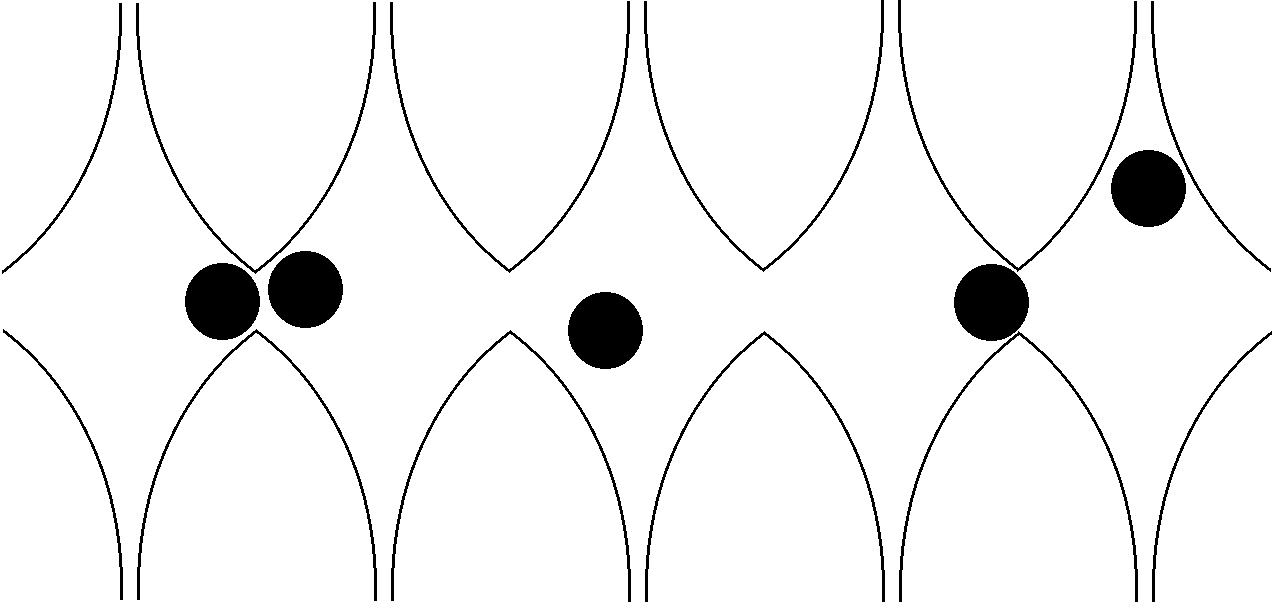
Figure 2. Particles are confined in a chain of cells.

As probably the simplest deterministic microscopic heat conduction model, the locally confined particle system is studied in various literatures. For example, under certain assumptions, the ergodicity of this model has been proved in [6]. Further rigorous investigation of the locally confined particle system is known to be difficult. Each cell in the locally confined particle system is a chaotic billiard table. And chaotic billiards are known to have many stochastic properties. Therefore, a natural strategy is to use a Markov process to approximate the change of particle energy in the locally confined particle system.

In [29], numerical simulations of first particle-particle collision in the locally confined particle system shows that for a pair of adjacent particles with energy $(E_{1},E_{2})$, the first particle-particle collision time has an exponential tail with slope $R(E_{1},E_{2})$. In addition, when $\min\{E_{1},E_{2}\}\ll 1$, we have $R(E_{1},E_{2})\sim\sqrt{\min\{E_{1},E_{2}\}}$. The heuristic justification of this rate is that when a particle has low energy, it has to move to the gate between cells by itself in order to have the next energy exchange. Hence a very slow particle dominates the next particle-particle collision time. If in addition we assume energy exchange in a particle-particle collision is done in a “random halves” way, we have a stochastic energy exchange model described in the next subsection.

5.2. Model Description

Consider a chain of $N$ linearly ordered lattice sites $\{1,2,\cdots,N\}$, each storing a fixed amount of energy $e_{i}$, $i=1,2,\cdots,N$. The chain is connected to two heat baths at the ends with temperatures $T_{L}$ and $T_{R}$, respectively.

An exponential clock is associated with each pair of adjacent sites, with rate $R(e_{i},e_{i+1})=\sqrt{\text{min}\{e_{i},e_{i+1}\}}$, called the stochastic energy exchange rate. Two clocks are associated with the ends of the chain and the heat baths. The clock between the left (resp. right) heat bath and the first (resp. last) site has a rate $\sqrt{\min\{T_{L},e_{1}}\}$ (resp. $\sqrt{\min\{T_{R},e_{N}}\}$).

When the $i$-th clock rings, sites $i$ and $i+1$ exchange energy as

$$(e_{i}^{\prime},e_{i+1}^{\prime})=(p(e_{i}+e_{i+1}),(1-p)(e_{i}+e_{i+1}))\,,$$

where $p$ satisfies the uniform distribution on $(0,1)$ and is independent of everything else. When a clock involving heat bath rings, the corresponding site exchanges energy with an exponential random variable with mean $T_{L}$ (or $T_{R}$) in the same “random halves” fashion. This is to say, we have

$$e_{1}^{\prime}=p(e_{1}+\rho_{L}),\quad\phi_{L}\sim Exp(T_{L})$$

and

$$e_{N}^{\prime}=p(e_{N}+\rho_{R}),\quad\rho_{R}\sim Exp(T_{R})\,,$$

where $p$ still satisfies the uniform distribution on $(0,1)$ and is independent of everything else. For the sake of simplicity, clocks at left and right boundaries are denoted by clock $0$ and clock $N+1$, respectively.

It is easy to see that the stochastic energy exchange model generates a Markov jump process $\mathbf{E}_{t}=(e_{1}(t),\cdots,e_{N}(t))$ on $\mathbb{R}^{N}_{+}$, where $e_{i}(t)$ represents the site $i$ energy at time $t$. We denote the transition kernel of $\mathbf{E}_{t}$ by $P^{t}(\mathbf{E},\cdot)$ for $\mathbf{E}\in\mathbb{R}^{N}_{+}$.

Let $h>0$ be a fixed number that represents the step size. The time-$h$ sampling chain of $\mathbf{E}_{t}$ is denoted by $\mathbf{E}^{h}_{n}$, or simply $\mathbf{E}_{n}$ when it does not lead to a confusion. The transition kernel of $\mathbf{E}_{n}$ is denoted by $P(\mathbf{E},\cdot)$.

5.3. Verifying (A1) and (A2).

We will first work on the time-$h$ chain $\mathbf{E}_{n}$. The verification of analytical conditions of $\mathbf{E}_{n}$ is based on the following Theorem.

Theorem 5.1.

For any set $K\subset\mathbb{R}^{N}_{+}$ of the form $K=\{(e_{1},\cdots,e_{N})\,|\,0<c_{i}\leq e_{i}\leq C_{i},i=1\sim N\}$ and any $h>0$, there exists a constant $\eta>0$ such that

$$P(\mathbf{E},\cdot)>\eta U_{K}(\cdot)\,,$$

for any $\mathbf{E}\in K$, where $U_{K}$ is the uniform probability distribution over $K$.

Proof.

For $\mathbf{E}=\{e_{1},\ldots,e_{N}\}\in K$ and $\mathrm{d}\mathbf{E}=\{(\mathrm{d}e_{1},\cdots,\mathrm{d}e_{N}),de_{i}>0,i=1\sim N\}$. Assume $\mathrm{d}e_{i}$s are sufficiently small. Let

$$B(\mathbf{E},\mathrm{d}\mathbf{E})=\{(x_{1},\cdots,x_{N})\in\mathbb{R}^{N}\,|\,e_{i}\leq x_{i}\leq e_{i}+\mathrm{d}e_{i}\})$$

denote the hypercube in $\mathbb{R}^{N}$. It then suffices to prove that for any $\mathbf{E}_{0}=\{\bar{e}_{1},\cdots,\bar{e}_{N}\}\in K$, we have

(5.1) $$P(\mathbf{E}_{0},B(\mathbf{E},d\mathbf{E}))>\sigma\mathrm{d}e_{1}\mathrm{d}e_{2}\cdots\mathrm{d}e_{N}\,,$$

where $\sigma$ is a strictly positive constant that is independent of $\mathbf{E}$ and $\mathbf{E}_{0}$.

We will then construct a sequence of events to go from the state $\mathbf{E}_{0}$ to $B(\mathbf{E},\mathrm{d}\mathbf{E})$ with desired positive probability. Let $\delta=\frac{h}{2N+1}$ and let $\epsilon>0$ be sufficiently small such that $\epsilon<\min\{c_{i},i=1\sim N\}$. Let $H=\sum_{i=1}^{N}e_{i}+\mathrm{d}e_{i}$. We consider the events $S_{1}\cdots,S_{N}$ and $F_{1},\ldots,F_{N+1}$, where $S_{i}$ and $F_{j}$ specifies what happens on the time interval $(i\delta,(i+1)\delta]$ and $(N\delta+(j-1)\delta,N\delta+j\delta]$, respectively.

• $S_{i}=$ $\{e_{i}(i\delta)\in[\epsilon/2,\epsilon]\}$ and { the $i$-th clock rings exactly once, all other clocks are silent on $((i-1)\delta,i\delta]$ }.

• $F_{1}=$ Energy emitted by right heat bath $\in(H,2H)$ and the $N$-th clock rings exactly once, all other clocks are silent on $(N\delta,(N+1)\delta]$ .

• $F_{j}=$ $\{e_{j}(N\delta+j\delta)\in[e_{N+2-j},e_{N+2-j}+\mathrm{d}e_{j}]\}$ and $\{$ the $(N+1-j)$-th clock rings exactly once, all other clocks are silent on $(N\delta+(j-1)\delta,N\delta+j\delta]$ $\}$ for $j=2,\cdots,N+1$.

The idea is that the energy at each site is first transported to the right heat bath, with only an amount of energy between $\epsilon/2$ and $\epsilon$ left at each site. Then a sufficiently large amount of energy is injected into the chain from the right heat bath so that it is always possible for site $j$ to acquire an amount of energy between $e_{j}$ and $e_{j}+\mathrm{d}e_{j}$ by passing the rest to site $j-1$, where sites $0$ and $N+1$ denote the left and right heat baths respectively.

It is easy to show that the probability of occurence of the sequence of events described above is always strictly positive. Here is a brief list of considerations. We will leave detailed calculations to the reader.

1. At each clock tick, we can give a lower bound on the rate of the $i^{th}$ clock (i.e., $\sqrt{\text{min}\{e_{i},e_{i+1}\}}$), since $0<\epsilon/2\leq e_{i}$ for all $i=1\sim N$ throughout the entire event.

2. Let $p\in(0,1)$ be the fraction in the mixing that puts $e_{i}\in[\epsilon/2,\epsilon]$. From the rule of energy redistribution, we need $\epsilon/2\leq p(e_{i}+e_{i+1})\leq\epsilon$. Rearrange the terms to get $\epsilon/[2(e_{i}+e_{i+1})]\leq p\leq\epsilon/(e_{i}+e_{i+1})$. This is possible since $\epsilon\leq e_{i}+e_{i+1}\leq\sum_{i=1}^{N}C_{i}$. Hence probabilities of $S_{i}$ are strictly positive.

3. There is also a uniform upper bound on $H$ given by $2\sum_{i=1}^{N}C_{i}$.

4. Let $p\in(0,1)$ be the fraction in the mixing that puts $e_{j}\in(e_{j},e_{j}+\mathrm{d}e_{j})$. From the rule of energy redistribution, we have $e_{j}/(e_{j-1}+e_{j})\leq p\leq(e_{j}+de_{j})/(e_{j-1}+e_{j})$. Because of $\epsilon\leq e_{j-1}+e_{j}\leq\sum_{i=1}^{N}C_{i}$ and $\mathrm{d}e_{j}>0$, $\mathbb{P}[e_{j}(N\delta+j\delta)\in[e_{N+2-j},e_{N+2-j}+\mathrm{d}e_{j}]]>\alpha\mathrm{d}e_{j}$ for some strictly positive constant $\alpha$. Hence probabilities of $F_{j}$ are greater than $\mathrm{const}\cdot\mathrm{d}e_{j}$.

In addition, all these probabilities are uniformly bounded from below for all $\mathbf{E}$ and $\bar{\mathbf{E}}$ in $K$. Hence we have

$$\mathbb{P}[S_{1}\cdots S_{N}F_{1}\cdots F_{N+1}]\geq\sigma\mathrm{d}e_{1}\cdots\mathrm{d}e_{N}$$

for some constant $\sigma>0$. ∎

As a corollary, we can prove that $\mathbf{E}_{n}$ is both aperiodic and irreducible with respect to the Lebesgue measure.

Corollary 5.2.

$\mathbf{E}_{n}$ is a strongly aperiodic Markov chain.

Proof.

By theorem 5.1, $K$ is a uniform reference set. In addition $U_{K}(K)>0$. The strong aperiodicity follows from its definition. ∎

Therefore $\mathbf{E}_{n}$ is aperiodic.

Corollary 5.3.

$\mathbf{E}_{n}$ is $\lambda$-irreducible, where $\lambda$ is the Lebesgue measure on $\mathbb{R}^{N}_{+}$.

Proof.

Let $A\subset\mathbb{R}^{N}_{+}$ be a set with strictly positive Lebesgue measure. Then there exists a set $K$ that has the form $\{(e_{1},\cdots,e_{N}\}\,|\,0<c_{i}\leq e_{i}\leq C_{i},i=1\sim N\}$ and $U_{K}(K\cap A)>0$.

For any $\mathbf{E}_{0}\in\mathbb{R}^{N}_{+}$ and the time step $h>0$, we can choose a $K\subset\mathbb{R}^{N}_{+}$ of the form $K=\{(e_{1},\cdots,e_{N}\}\,|\,0<c_{i}\leq e_{i}\leq C_{i},i=1\sim N\}$ for some $c_{i}>0$ and $C_{i}<\infty$, such that $\mathbf{E}_{0}\in K$. Same construction as in Theorem 5.1 implies that $P^{h}(\mathbf{E}_{0},\cdot)>\eta U_{K}(\cdot)$ for some $\eta>0$. Therefore, $P^{h}(\mathbf{E}_{0},A)>\eta U_{K}(A)>0$.

∎

Hence assumption (A1) and (A2) are satisfied.

5.4. Absolute continuity of invariant measure.

This subsection aims to prove the absolute continuity of $\pi$ with respect to the Lebesgue measure, which is denoted by $\lambda$.

Proposition 5.4.

If $\pi$ is an invariant measure of $\mathbf{E}_{t}$, then $\pi$ is absolutely continuous with respect to $\lambda$ with a strictly positive density.

For $\mathbf{E}\in\mathbb{R}^{N}_{+}$ and $t>0$, we have decomposition

$$P^{t}(\mathbf{E},\cdot)=\nu_{\perp}+\nu_{abs}\,,$$

where $\nu_{abs}$ and $\nu_{\perp}$ are absolutely continuous and singular component with respect to $\lambda$, respectively. We need to show that an absolutely continuous component cannot revert back to singularity as time evolves.

Lemma 5.5.

For any probability measure $\mu\ll\lambda$, $\mu P^{t}\ll\lambda$ for any $t>0$.

Proof.

This proof is essentially identical to that of Lemma 6.3 of [31]. All what we need to prove is that, for any absolutely continuous initial distribution, the push-forward measure corresponding to one clock ringing is still absolutely continuous. We refer readers to [31] for the detailed calculations. ∎

Proof of Proposition 5.4. .

Let $\pi=\pi_{abs}+\pi_{perp}$ be an invariant measure. Assume $\pi_{perp}\neq 0$. For $t>0$, $\pi_{abs}P^{t}\ll\lambda$ by Lemma 5.5. By Theorem 5.1, for any $\mathbf{E}\in\mathfrak{C}$, $P^{t/2}(\mathbf{E},\cdot)$ has a strictly positive density on $\mathfrak{C}$. Since $\mathfrak{C}$ is accessible within finitely many energy exchanges, $P^{t/2}(\mathbf{E},\mathfrak{C})>0$ for all $\mathbf{E}\in\mathbb{R}^{N}_{+}$. Hence $P^{t}(\mathbf{E},\cdot)$ has a strictly positive density on $\mathfrak{C}$ for all $\mathbf{E}\in\mathbb{R}^{N}_{+}$. Therefore, $\pi_{\perp}P^{t}$ has an absolutely continuous component. The absolutely continuous component of $\pi P^{t}$ is strictly larger than that of $\pi$. This contradicts with the invariance of $\pi$.

∎

5.5. Verifying (N1) and (N2).

Now we are ready to present our numerical results. We let $N=3$ in our simulations. The uniform reference set $\mathfrak{C}$ is chosen as

$$\mathfrak{C}=\{(e_{1},\cdots,e_{N})\,|\,0.1\leq e_{i}\leq 100,i=1\sim N\}\,.$$

Throughout our numerical justification, we let $h=0.1$. (Recall that for a time-continuous Markov process $\Psi_{t}$, the definition of $\tau_{\mathfrak{C}}=\tau_{\mathfrak{C}}(h)$ depends on $h$.) We will verify (N1) for the numerical invariant measure, which is generated by running the process for a sufficiently long time from a suitable initial distribution. In our simulation, the initial distribution for the simulation of the numerical invariant measure is $\mu_{0}\sim(\rho_{1},\cdots,\rho_{N})$, where $\rho_{i}$ is an exponential distribution with mean $(T_{L}+T_{R})/2$. We find that when $T=200$, expectations of many observables we have tested are stabilized (Figure 3 ). Therefore, the numerical invariant measure is chosen as $\hat{\pi}:=\mu_{0}P^{200}$. Then from the result of our simulation that chooses the numerical invariant measure as the specific starting state, we conclude that $\mathbb{P}_{\hat{\pi}}[\tau_{\mathfrak{C}}>t]\sim t^{-2}$. (Figure 4 ).

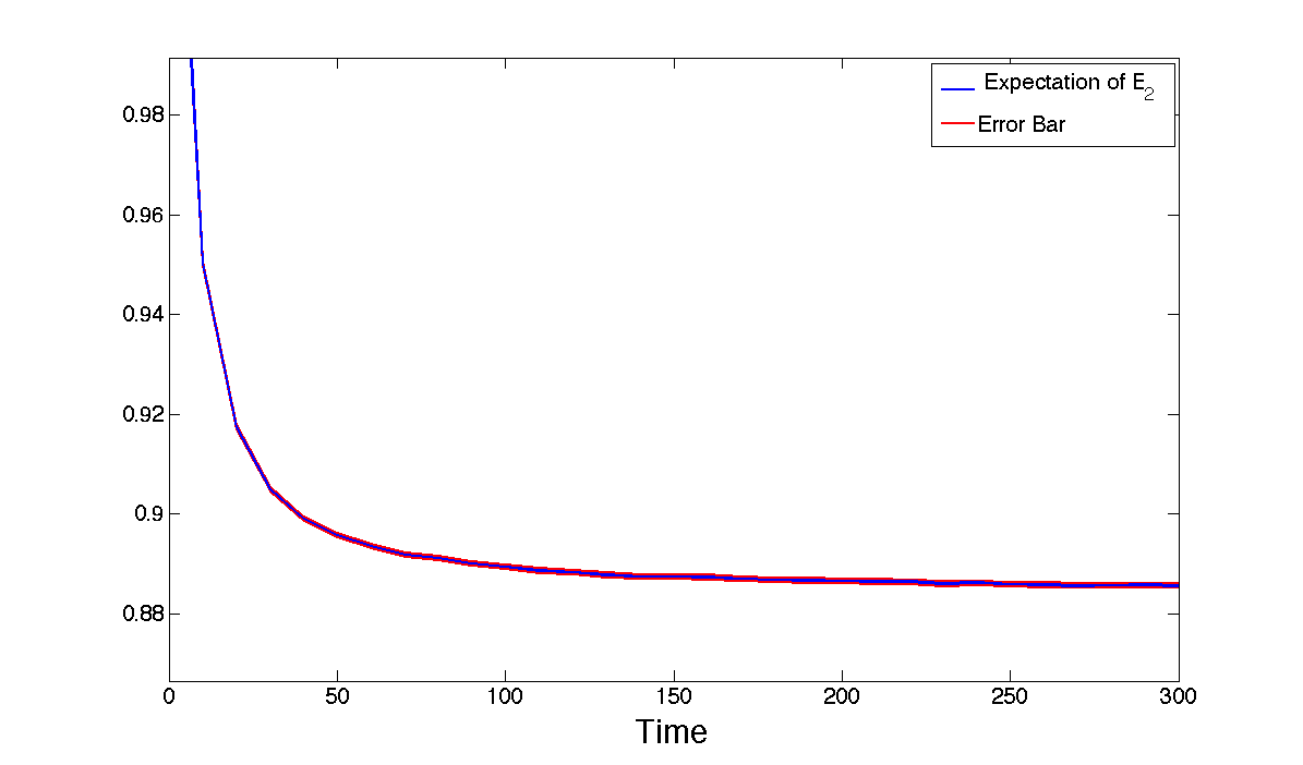
Figure 3. Expectation of energy at site $2$ verses time. Sample size $M=1\times 10^{8}$. The error bar represents $\pm 1.96M^{-1/2}$ times the sample standard deviation.

It remains to check (N2). The transition kernel of the time-$h$ sample chain of $\mathbf{E}_{t}$ does not have a clean explicit form. In addition, the transition kernel of $\mathbf{E}_{t}$ has many singularities. As a result, proving the condition in Proposition 3.3 is an extremely tedious work. Instead, we choose to numerically show that

$$\gamma(\mathbf{E})=\sup_{t\geq h}\frac{\mathbb{P}_{\mathbf{E}}[\tau_{\mathfrak{C}}>t]}{t^{-2}}$$

is uniformly bounded on $\mathfrak{C}$. We follow procedure (a)-(d) in Section 3 to show the boundedness of $\gamma(\mathbf{E})$. In fact,

$$\gamma_{N}(\mathbf{E})=\sup_{1\leq n\leq N}\sup_{t\geq h}\frac{\mathbb{P}_{\mathbf{E}}[\tau_{\mathfrak{C}}>t]}{t^{-2}}$$

is stabilized very fast with increasing $N$. A sample of size $10^{6}$ is sufficient for a reliable estimate of $\gamma(\mathbf{E})$. Figure 6 shows that when $E_{i}$ is small, $\gamma(\mathbf{E})$ decreases monotonically with decreasing $E_{i}$ for each $i=1\sim 3$. Therefore, we expect that the maximal of $\gamma(\mathbf{E})$ in $\mathfrak{C}$ is reached at $\mathbf{E}_{*}=(0.1,0.1,0.1)$. In fact, intuitively one should expect $\gamma(\mathbf{E})$ to decrease with site energy as starting from low site energy means having higher probability to have even lower site energy after an energy exchange. Finally, we run the simulation again to estimate $\gamma(\mathbf{E}_{*})$. As seen in Figure 6, when starting from $\mathbf{E}_{*}$ the probability of return has tail $\sim t^{-2}$. ($\gamma(\mathbf{E}_{*})$ is approximately $48.8915$ with standard deviation $0.0225$.)

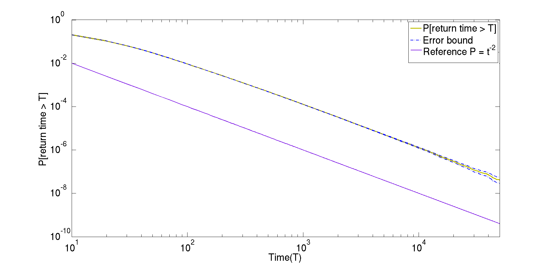
Figure 4. $\mathbb{P}_{\hat{\pi}}[\tau_{\mathfrak{C}}>t]$, $\pi$ is the numerical steady state obtained from long time averaging. Sample size $=1\times 10^{8}$. The purple line is a reference line with slope $-2$. The error bar is calculated as in Remark 3.5.

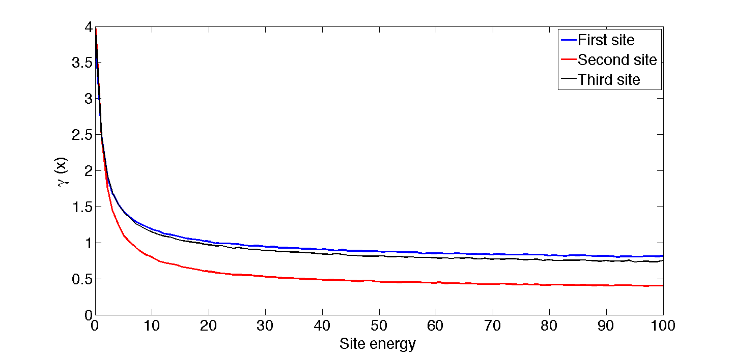
Figure 5. Change of $\gamma(\mathbf{E})$ for varying $\mathbf{E}$ when only one site energy changes. The unchanged site energy is set to be $1$. Sample size $=10\times 1\times 10^{7}$ for each initial condition.

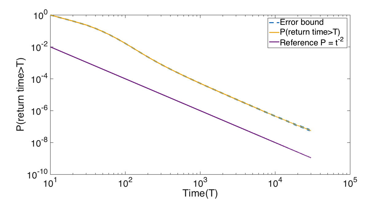
Figure 6. $\mathbb{P}_{\mathbf{E}_{*}}[\tau_{\mathfrak{C}}>t]$ for $\mathbf{E}_{*}=(0.1,0.1,0.1)$. Sample size $=1\times 10^{10}$. The purple line is a reference line with slope $-2$. The error bar is calculated as in Remark 3.5.

5.6. Main conclusions.

The previous subsection verifies both (N1) and (N2) for $\bf{E}_{t}$ with parameter 2. The slope of $\mathbb{P}_{\hat{\pi}}[\tau_{\mathfrak{C}}>t]$ in the log-log plot is $2$. Note that $\mathbb{P}[\Psi_{t}=\Psi_{0}\,|\,\Psi_{0}\in K]=\mathbb{P}_{\Psi_{0}}[\mbox{ no clock rings up to }t]$ is uniformly positive for each given $t>0$. By Theorem 4.5, (N1) and (N2) hold for $\mathbf{E}_{n}$ with parameter $2-\epsilon/2$ for arbitrarily small $\epsilon>0$. Therefore, conclusions (a)-(d) in Section 4.4 hold for $\mathbf{E}_{n}$.

It remains to pass the results for $\mathbf{E}_{n}$ to $\mathbf{E}_{t}$. By Proposition 4.3, it is sufficient to prove “continuity at zero” for $\mathbf{E}_{t}$.

Lemma 5.6.

For any probability measure $\mu$ on $\mathbb{R}^{N}_{+}$,

$$\lim_{\delta\rightarrow 0}\|\mu P^{\delta}-\mu\|_{TV}=0$$

Proof.

It is sufficient to prove that for any $\epsilon>0$, there exists a $\delta>0$ such that

$$\|\mu P^{\delta}-\mu\|_{TV}\leq\epsilon\,.$$

Since $\mu$ is finite, there exists a bounded set $A\subset\mathbb{R}^{N}_{+}:=\{0\leq E_{i}\leq M\}$ such that $\mu(A)>1-\epsilon/4$. By the definition of $A$, clock rates for initial values in $A$ are uniformly bounded. Therefore, one can find a sufficiently small $\delta>0$, such that $\mathbb{P}[\mbox{ no clock rings on }[0,\delta)]\geq 1-\epsilon/4$. For any set $U\subset\mathbb{R}^{N}_{+}$, we have

$$(\mu P^{\delta})(U) = \int_{\mathbb{R}^{N}_{+}}P^{\delta}(\mathbf{E},U)\mu(\mathrm{d}\mathbf{E})$$

$$= \int_{A\cap U}P^{\delta}(\mathbf{E},U)\mu(\mathrm{d}\mathbf{E})+\int_{A-U}P^{\delta}(\mathbf{E},U)\mu(\mathrm{d}\mathbf{E})+\int_{A^{c}}P^{\delta}(\mathbf{E},U)\mu(\mathrm{d}\mathbf{E})$$

$$= \mu(A\cap U)-a_{1}+a_{2}+a_{3}\,,$$

where

$$a_{1} = \int_{A\cap U}(1-P^{\delta}(\mathbf{E},U))\mu(\mathrm{d}\mathbf{E})\leq\frac{\epsilon}{4}\mu(A\cap U)\leq\frac{\epsilon}{4}$$

$$a_{2} = \int_{U-A}P^{\delta}(\mathbf{E},U)\mu(\mathrm{d}\mathbf{E})\leq\frac{\epsilon}{4}\mu(A-U)\leq\frac{\epsilon}{4}$$

$$a_{3} = \int_{A^{c}}\frac{\epsilon}{4}\mu(A\cap U)\leq\frac{\epsilon}{4}\mu(A^{c})\leq\frac{\epsilon}{4}\,.$$

In addition we have $\mu(U)-\mu(A\cap U)\leq\mu(A^{c})<\frac{\epsilon}{4}$. Hence

$$|(\mu P^{\delta})(U)-\mu(U)|<\epsilon$$

for any $U\subset\mathbb{R}^{N}_{+}$. By the definition of the total variation norm, we have

$$\|\mu P^{\delta}-\mu\|\leq\epsilon\,.$$

This completes the proof.

∎

We haven’t talked about uniqueness so far. Usually the uniqueness of the invariant probability measure follows from the fact that $P(x,\cdot)$ admits positive density everywhere.

Proposition 5.7.

For any $h>0$, $\mathbf{E}^{h}_{n}$ admits at most one invariant probability measure.

Proof.

By the proof of Theorem 5.1, for any $\mathbf{E}\in K$, $P^{h/2}(\mathbf{E},\cdot)$ has strictly positive density on $K$. In addition, $P^{h/2}(\mathbf{E}_{0},K)>0$ for any $\mathbf{E}_{0}\in\mathbb{R}^{N}_{+}$. Hence $P^{h}(\mathbf{E}_{0},\cdot)$ has positive density on $K$. This implies that every $\mathbf{E}_{0}\in\mathbb{R}^{N}_{+}$ belongs to the same ergodic component. Therefore $\mathbf{E}^{h}_{n}$ cannot have more than one invariant probability measure. ∎

In summary, we have the following conclusions for $\mathbf{E}_{t}$.

1. For any $T_{L}$, T_R, there exists a unique invariant probability measure $\pi$, i.e., the nonequilibrium steady-state, which is absolutely continuous with respect to the Lebesgue measure on $\mathbb{R}^{N}_{+}$.

2. For almost every $\mathbf{E}_{0}\in\mathbb{R}^{N}_{+}$ and any sufficiently small $\epsilon>0$, we have

   $$\lim_{t\rightarrow\infty}t^{2-\epsilon}\|\delta_{\mathbf{E}_{0}}P^{t}-\hat{\pi}P^{t}\|_{TV}=0\,.$$

3. For any functions $\eta$, $\xi\in L^{\infty}(\mathbf{R}^{N}_{+})$, we have

   $$C_{\pi}^{\eta,\xi}(t)\leq O(1)\cdot t^{\epsilon-2}$$

   for any $\epsilon>0$.

6. Example: random halves model

6.1. Derivation from deterministic dynamics

Another way to simplify the multi-body problem as described in Figure 1 at the beginning of the previous section is to assume that particles do not interact directly. Instead, we divide the tube into a chain of $N$ cells, each of which contains a rotating disk that plays the role of the “local environment”. As seen in Figure 7, particles can only exchange energy with the rotating disk. Then we connect this chain with two thermalized ends, called heat baths, such that thermalized particles can be injected into the system and particles in the system can exit by entering the heat bath. This is the Hamiltonian model proposed in [14]. We refer [14, 31] for details.

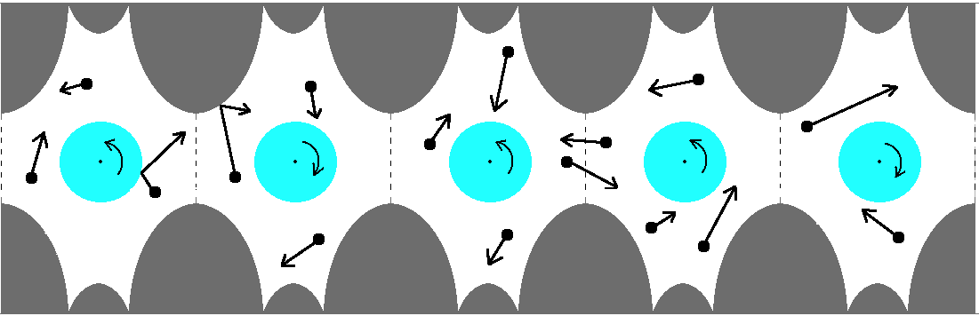
Figure 7. Moving particles do not interact with each other directly. There is a rotating disk with fixed center in each cell. The collision between particles and disks are determined by the conservation of kinetic energy and angular momentum.

A particle in this Hamiltonian model has chaotic trajectories and quick loss of “memory”. Therefore, it is natural to assume that the movement of each particle is stochastic, i.e., governed by an energy dependent exponential clock. When a clock associated with a particle rings, the particle either jumps to neighboring cells or exchanges energy with the local environment. The probability of occurence of either event is a constant determined by the system. This reduces the Hamiltonian model to the so-called random halves model, which is described in the next subsection. We refer [31] for the full detail of this model reduction process and a brief justification of the model reduction.

6.2. Model Description

Consider $N$ linearly ordered lattice sites$\{1,2,\cdots,N\}$, each containing an energy tank and storing a finite number of particles with certain amount of energy. The lattice sites are connected to two heat baths at the ends, denoted as sites $0$ and $N+1$ for the sake of simplicity. The heat baths have temperatures $T_{L}$ and $T_{R}$, as well as exponential particle injection rates of $\rho_{L}$ and $\rho_{R}$, respectively. Particle energies are random variables with i.i.d. distributions with a probability density function

$$\frac{2}{\sqrt{\pi}T^{3/2}}\sqrt{x}e^{-\frac{x}{T}}$$

where $T$ is the temperature of the heat bath from which the particle is emitted. Notice that when a particle is emitted by the left heat bath, it instantaneously appears at site 1. When a particle is emitted by the right heat bath, it instantaneously appears at site N.

An exponential clock is associated with each particle in the system, with rate $(1+m)S\sqrt{x}$, where $x$ is the energy of the particle and $m$ and $S$ are system constants. When the clock of a particle rings, the particle jumps with probability $\frac{1}{1+m}$ and “mixes” with probability $\frac{m}{1+m}$. Rules for jumping and “mixing” for a particle at site $i$ carrying energy $x_{j}^{i}$, where $j$ is the index of the particle in its site, are as follows.

When a particle jumps, it goes to either site $i+1$ or site $i-1$ with equal probability of $\frac{1}{2}$. Let $k_{i}$ be the number of particles at site $i$. Then $k_{i}$ decreases by 1 while the site that the particle jumps to has an increase in particle number by 1. Notice that the particle leaves the system if it jumps to the left or right heat bath. For “mixing”, we mean a particle exchanges energy with the stored energy at its site. Let $s_{i}$ be the stored energy at site $i$ and let $x_{j}$ be the corresponding particle energy. The rule of energy exchange is $(s_{i}^{\prime},x^{\prime}_{j})=(x_{j}u^{2},s_{i}+x_{j}(1-u^{2}))$, where u is a uniform random variable distributed on $(0,1)$.

Random halves model generates a Markov jump process

$$\mathbf{\omega}_{t}=((s_{1}(t),\{x_{1}^{1}(t),\ldots,x_{k_{1}}^{1}(t)\}),\ldots,(s_{N}(t),\{x_{1}^{N}(t),\ldots,x_{k_{N}}^{N}(t)\})),$$

where $k_{1},\ldots,k_{N}$ take values in $\mathbb{N}\cup\{0,\infty\}=\{0,1,\ldots,\infty\}$. The stochastic process takes values in the state space $\Omega=\Pi_{i=1}^{N}\Omega^{i}$, where $\Omega^{i}=\cup_{k=0}^{\infty}\Omega_{k}^{i}$, and $\Omega_{k}^{i}=\{(s_{i},\{x^{i}_{1},\ldots,x^{i}_{k}\})|s_{i},x^{i}_{j}>0\}$. Since we regard particles as indistinguishable to avoid confusion when particles re-enter the system, we use unordered lists denoted by curly brackets. Notice that $\Omega_{k}^{i}=\mathbb{R}_{+}\times((\mathbb{R}_{+})^{k}/\sim)$, where $\sim$ is the equivalence relation given by $\{x_{1},\ldots,x_{k}\}\sim\{x_{\sigma_{1}},\cdots,x_{\sigma_{k}}\}$, $\sigma$ is any $k$-permutation.

Therefore, we can define the Markov jump process $\omega(t)$ generated by random halves model on $\Omega$. We denote the transition kernel of $\omega(t)$ by $P^{t}(\mathbf{\omega},\cdot)$. Let $h>0$ be a fixed number that represents the step size. The time-$h$ sampling chain of $\mathbf{\omega}_{t}$ is denoted by $\mathbf{\omega}^{h}_{n}$, or simply $\mathbf{\omega}_{n}$ when it does not lead to a confusion. The transition kernel of $\mathbf{\omega}_{n}$ is denoted by $P(\mathbf{\omega},\cdot)$.

For the sake of later use, we will define a reference measure $\Lambda$ on $\Omega$, where $\Lambda=\prod_{1}^{N}\Lambda_{i}$ and $\Lambda_{i}$ is the natural reference measure on $\Omega^{i}$, such that the restriction of $\Lambda_{i}$ on $\Omega^{i}_{k}$ is the quotient of the Lebesgue measure on $\mathbb{R}\times\mathbb{R}^{k}$ under the relationship $\sim$.

6.3. Verifying (A1) and (A2).

We will first work on the time-$h$ sampling chain of $\mathbf{\omega}_{n}$. The verification of analytical conditions of $\mathbf{\omega}_{n}$ is based on the following theorem.

Theorem 6.1.

For any set $K\subset\Omega$, of the form $\{\omega\in\Omega|0\leq k_{i}\leq K_{0},0\leq s_{i}\leq S_{0},c\leq x^{i}_{j}\leq C,i=1\sim N,j=1\sim k_{i}\}$, where $K_{0},S_{0},c,C$ are positive constants, and any $h>0$, there exists a constant $\eta>0$ such that

$$P(\omega,\cdot)>\eta\Lambda_{K}(\cdot),$$

for all $\omega\in K$, where $\Lambda_{K}$ is the reference measure restricted to $K$.

Proof.

For $\omega=((\hat{s}_{1},\{\hat{x}_{1}^{1},\ldots,\hat{x}_{k_{1}}^{1}\}),\ldots,(\hat{s}_{N},\{\hat{x}_{1}^{N},\ldots,\hat{x}_{k_{N}}^{N}\}))\in K$, let $A_{\omega}(ds)=\{(s_{1},\{x_{1}^{1},\ldots,x_{k_{1}}^{1}\}),\ldots,(s_{N},\{x_{1}^{N},\ldots,x_{k_{N}}^{N}\}))|\hat{s}_{1}\leq s_{1}\leq\hat{s}_{1}+ds,\ldots,\hat{s}_{N}\leq s_{N}\leq\hat{s}_{N}+ds,\hat{x}_{j}^{i}\leq x_{j}^{i}\leq\hat{x}_{j}^{i}+ds,\text{ for }1\leq i\leq N,1\leq j\leq k_{i}\}$ for $ds\ll 1$.

It then suffices to prove that for each

$$\bar{\omega}=((\bar{s}_{1},\{\bar{x}_{1}^{1},\ldots,\bar{x}_{\bar{k}_{1}}^{1}\}),\ldots,(\bar{s}_{N},\{\bar{x}_{1}^{N},\ldots,\bar{x}_{\bar{k}_{N}}^{N}\}))\in K\,,$$

we have

$$P(\bar{\omega},A_{\omega}(ds))\geq\sigma ds^{1+k_{1}}\cdots ds^{1+k_{N}}$$

for $0<ds\ll 1$, where $\sigma$ is a strictly positive constant that is independent of $\bar{\omega}$ and $\omega$.

In order to do so, we will construct a sequence of events to go from the state $\bar{\omega}$ to $A_{\omega}(ds)$ with positive probability. Let $M=\sum_{i=1}^{N}k_{i}$ and $\bar{M}=\sum_{i=1}^{N}\bar{k}_{i}$. Let $\delta=\frac{h}{M+\bar{M}+N}$. And let $E=\sum_{i=1}^{N}(\hat{s}_{i}+ds)$. We consider the events $F_{i},G,H_{i},A_{i}$, where $i=1\sim N$.

• $F_{i}=\{\text{on }((i-1)\delta,i\delta],i=1\sim\bar{M}$, no new particle enters, and one particle present initially exits the system without exchanging energy $\}$.

• Define an auxiliary event $A_{i}=\{\hat{s}_{i}\leq s_{i}\leq\hat{s}_{i}+ds\}$ on $((M+i-1)\delta,(M+i)\delta]$.

• $H_{i}=A_{i}\cap$ $\{$ on $(M\delta+(i-1)\delta,M\delta+i\delta]$, exactly one particle, carrying energy on the interval $[E,2E]$, enters from the left and jumps through all sites $s_{j},j<i$ without exchanging energy, then exchanges energy with site $i$, and jumps to exit the system from the right $\}$ $\cap$ $\{$ no other new particle enters $\}$ for $i=M\sim M+N$.

• $G=$ $\{$ on $(i\delta,(i+1)\delta],i=\bar{M}+N\sim\bar{M}+N+M$, $k_{i}$ particles with energy $x_{j}^{i}\in[\hat{x}_{j}^{i},\hat{x}_{j}^{i}+ds]$ for $j=1\sim k_{i}$ enters the system from the left and jumps until reaching site $i$, without exchanging energy $\}$ $\cap$ $\{$ no new particle enters and existing particles do nothing $\}$.

The idea is that particles initially present at each site are first emptied from the system. Then for each site, one particle with sufficiently large amount of energy enters the system to mix at the corresponding site. Lastly, particles in the target set enter the system and jump to corresponding sites. We need to show that the probability of occurence of the sequence of events described above is always strictly positive. Here are the considerations.

1. The initial number of particles $k_{i}\leq K_{0}$ for each $i=1\sim N$. Clock rates $(1+m)S\sqrt{x_{j}^{i}}$ are bounded above zero since $x_{j}^{i}\geq c$, and bounded below infinity since $x_{j}^{i}\leq C$ by assumption. Hence $F_{i}$ occurs with strictly positive probability.

2. Let $u\in(0,1)$ be the fraction in the mixing that puts $s_{i}\in[\hat{s}_{i},\hat{s}_{i}+ds]$. Let $X$ be the particle energy in the event $H_{i}$. Rearrange the terms to get $\hat{s}_{i}/X\leq u^{2}\leq(\hat{s}_{i}+ds)/X$. Note that $X$ is bounded from above by $2NS_{0}$. Therefore, $\mathbb{P}[A_{i}]>\alpha ds$ for some constant $\alpha>0$.

3. In addition, during the event $\{H_{i},i=1\sim N\}$, $E$ is bounded from above by $NS_{0}$. The probability of $H_{i}$ is greater than $\mathrm{const}\cdot ds$.

4. The number of particles in the destination set $\bar{k}_{i}\leq K_{0}$ for each $i=1\sim N$, and clock rates are bounded both above from zero and below from $C$. Hence $G$ occurs with probability at least $\mathrm{const}\cdot ds^{k_{1}}\cdots ds^{k_{N}}$.

In addition, all these probabilities and probability densities are uniformly bounded from below for all $\bar{\omega}$ and $\omega$ in $K$. ∎

As a corollary, we can prove that $\omega_{n}$ is both aperiodic and irreducible with respect to the reference measure.

Corollary 6.2.

$\omega_{n}$ is a strongly aperiodic Markov chain.

Proof.

By 6.1, $K$ is a uniform reference set. In addition $\Lambda_{K}(K)>0$. The strong aperiodicity follows from its definition. ∎

Therefore $\omega_{n}$ is aperiodic.

Corollary 6.3.

$\omega_{n}$ is $\Lambda$-irreducible, where $\Lambda$ is the reference measure on $\Omega$.

Proof.

Let $A\subset\Omega$ be a set with strictly positive measure. Then there exists a set $U$ that has the form $U=\{\omega\in\Omega|0\leq k_{i}\leq K_{0},0\leq s_{i}\leq S_{0},c\leq x^{i}_{j}\leq C,i=1\sim N,j=1\sim k_{i}\}$ and $\Lambda_{K}(U\cap A)>0$.

For any $\omega_{0}\in\Omega$ and the time step $h>0$, there exists a set $K$ that has the form as in Theorem 6.1 such that $\omega_{0}\in K$. Hence same construction as in Theorem 6.1 implies that $P^{h}(\omega_{0},\cdot)>\eta\Lambda_{K}(\cdot)$ for some $\eta>0$. Therefore $P^{h}(\omega_{0},A)>\eta\Lambda_{K}(A)>0$. ∎

6.4. Absolute continuity of invariant measure

The proof of the absolute continuity of $\pi$ with respect to $\Lambda$ is similar as in the previous section.

Proposition 6.4.

If $\pi$ is an invariant measure of $\omega_{t}$, then $\pi$ is absolutely continuous with respect to $\lambda$ with a strictly positive density.

Proof.

Let $\pi=\pi_{abs}+\pi_{\perp}$ be an invariant measure, where $\pi_{abs}$ and $\pi_{\perp}$ are absolutely continuous and singular components with respect to $\Lambda$ respectively. Since $\pi_{abs}\ll\Lambda$, $\pi_{abs}P^{t}\ll\Lambda$ for any $t>0$ by Lemma 6.3 of [31]. For similar reasons as in the previous model, we again refer readers to [31] for detailed calculations. The rest of the proof then follows the same line as in the proof of Proposition 5.4. ∎

6.5. Verifying (N1) and (N2).

Now we will present our numerical results for the random halves model. We let $N=3$ or $4$, depending on the computational cost of the simulation. The uniform reference set $\mathfrak{C}$ is chosen as

$$\mathfrak{C}=\{\omega\in\Omega|0\leq k_{i}\leq 40,0\leq s_{i}\leq 100,0.1\leq x^{i}_{j}\leq 100,i=1\sim N,j=1\sim k_{i}\}$$

Throughout our numerical justification about $\tau_{\mathfrak{C}}=\tau_{\mathfrak{C}}(h)$, we let $h=0.1$. We very (N1) for the numerically generated invariant measure. The numerical invariant measure is generated by running the process for a sufficiently long time from a suitable initial distribution. In our simulation, the initial distribution for the simulation of the numerical invariant measure is

$$\omega_{0}\sim((s_{1}(t),\{x_{1}^{1}(t),\ldots,x_{k_{1}}^{1}(t)\}),\ldots,(s_{N}(t),\{x_{1}^{N}(t),\ldots,x_{k_{N}}^{N}(t)\}))\,,$$

where $N=3$, each $s_{i}$ is uniformly distributed between 0 and 100, each $k_{i}$ is a poisson distribution with mean $(\rho_{L}+\rho_{R})/2$, and each $x^{i}_{j}$ is an exponential distribution with mean $(T_{L}+T_{R})/2$. We find that when $T=100$, the expectation of the observables we have tested are stabilized (Figure 8). Therefore the numerical invariant measure is chosen as $\hat{\pi}:=\mu_{0}P^{100}$. Then from the result of our simulation that chooses the numerical invariant meausure as the specific starting state, we conclude that $\mathbb{P}_{\omega_{0}}[\tau_{\mathfrak{C}}>t]\sim t^{-2}$ and $\mathbb{P}_{\hat{\pi}}[\tau_{\mathfrak{C}}>t]\sim t^{-2}$. (Figure 9).

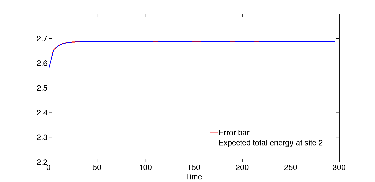
Figure 8. Total energy at the second site verses time. Sample size $M=1\times 10^{8}$. The error bar represents $\pm 1.96M^{-1/2}$ times the sample standard deviation.

It remains to check (N2). Same as in the previous section, the transition kernel of the time-$h$ sample chain does not have a clean explicit form. Hence we choose to numerically verify the boundedness of

$$\gamma(\omega)=\sup_{t\geq h}\frac{\mathbb{P}_{\omega}[\tau_{\mathfrak{C}}>t]}{t^{-2}}\,.$$

In this example, the uniform reference set $\mathfrak{C}$ has much higher dimension. But we can still numerically capture the monotonicity. Our simulation result shows that $\gamma(\omega)$ increases monotonically with decreasing site energy (Figure 11) and particle energy at each site (Figure 11), and increases monotonically with number of particles at each site (Figure 13). Therefore we expect the maximal of $\gamma(\omega)$ in $\mathfrak{C}$ to be $\omega_{*}=\{(0,\{0.1,\ldots,0.1\}),(0,\{0.1,\ldots,0.1\}),(0,\{0.1,\ldots,0.1\})\}$, for $k_{i}=40,i=1\sim 3$. This result matches the heuristic argument that lower site energy, lower particle energy, and higher number of particles at the initial condition produces higher probability of entering the low energy states. Finally, we run the simulation again with initial value $\omega_{*}$ to verify that the return time has tail $\sim t^{-2}$ in Figure 13. ($\gamma(\omega_{*})$ is approximately $1291.8695$ with standard deviation $5.3388$.)

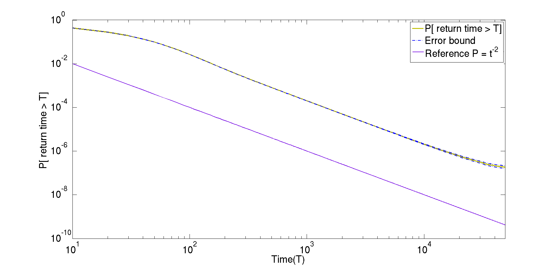
Figure 9. $\mathbb{P}_{\hat{\pi}}[\tau_{\mathfrak{C}}>t]$, $\pi$ is the numerical steady state obtained from long time averaging. Sample size = $1\times 10^{8}$. The purple line is a reference line with slope $-2$. The error bar is calculated as in Remark 3.5.

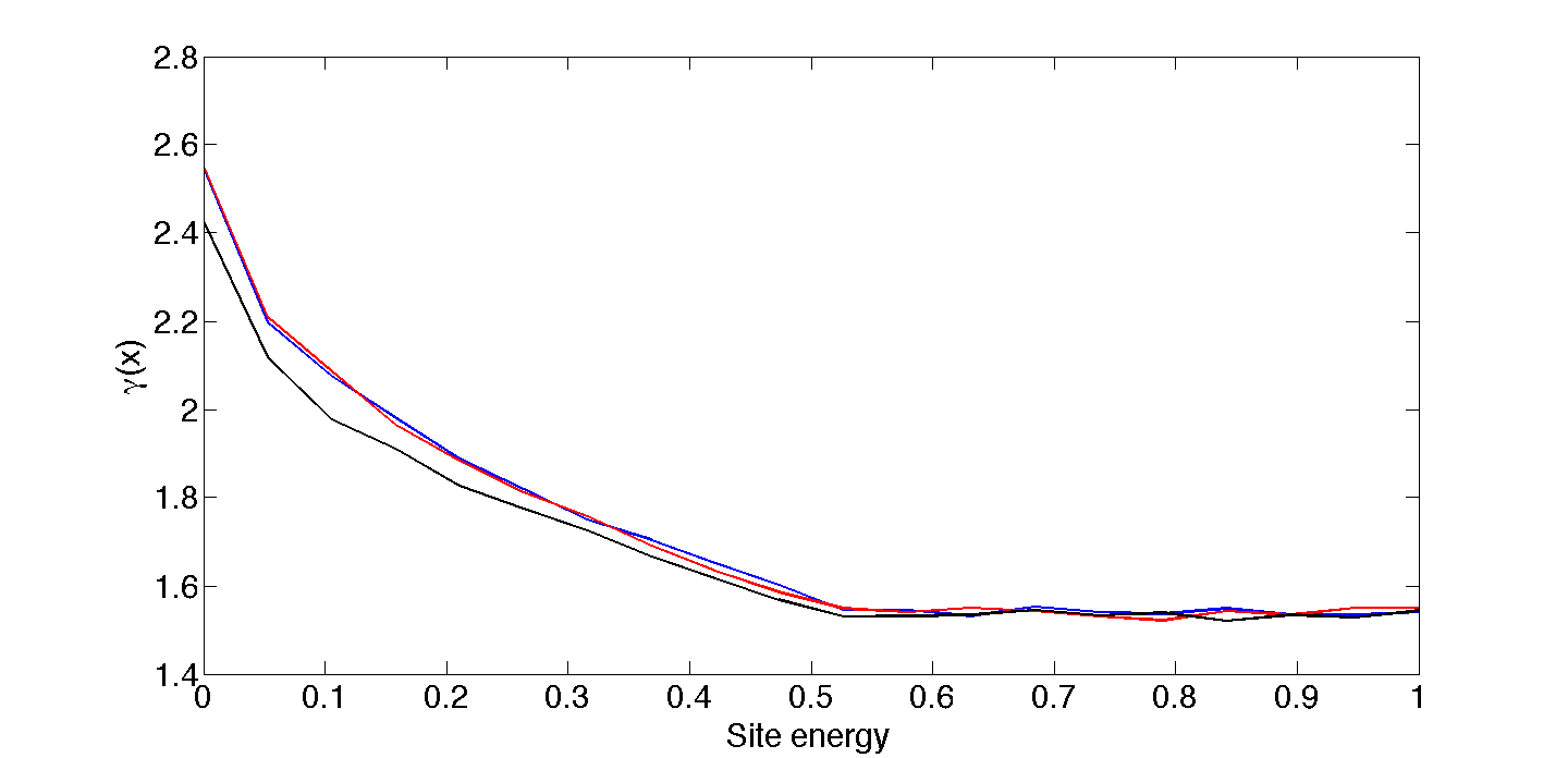
Figure 10. Change of $\gamma(\omega)$ for varying $\omega$ when site energy at only one site changes. The energy configuration of an unchanged site is: site energy $=1$, two particles per site with particle energy = $1$. Sample size = $1\times 10^{7}$ for each initial condition.

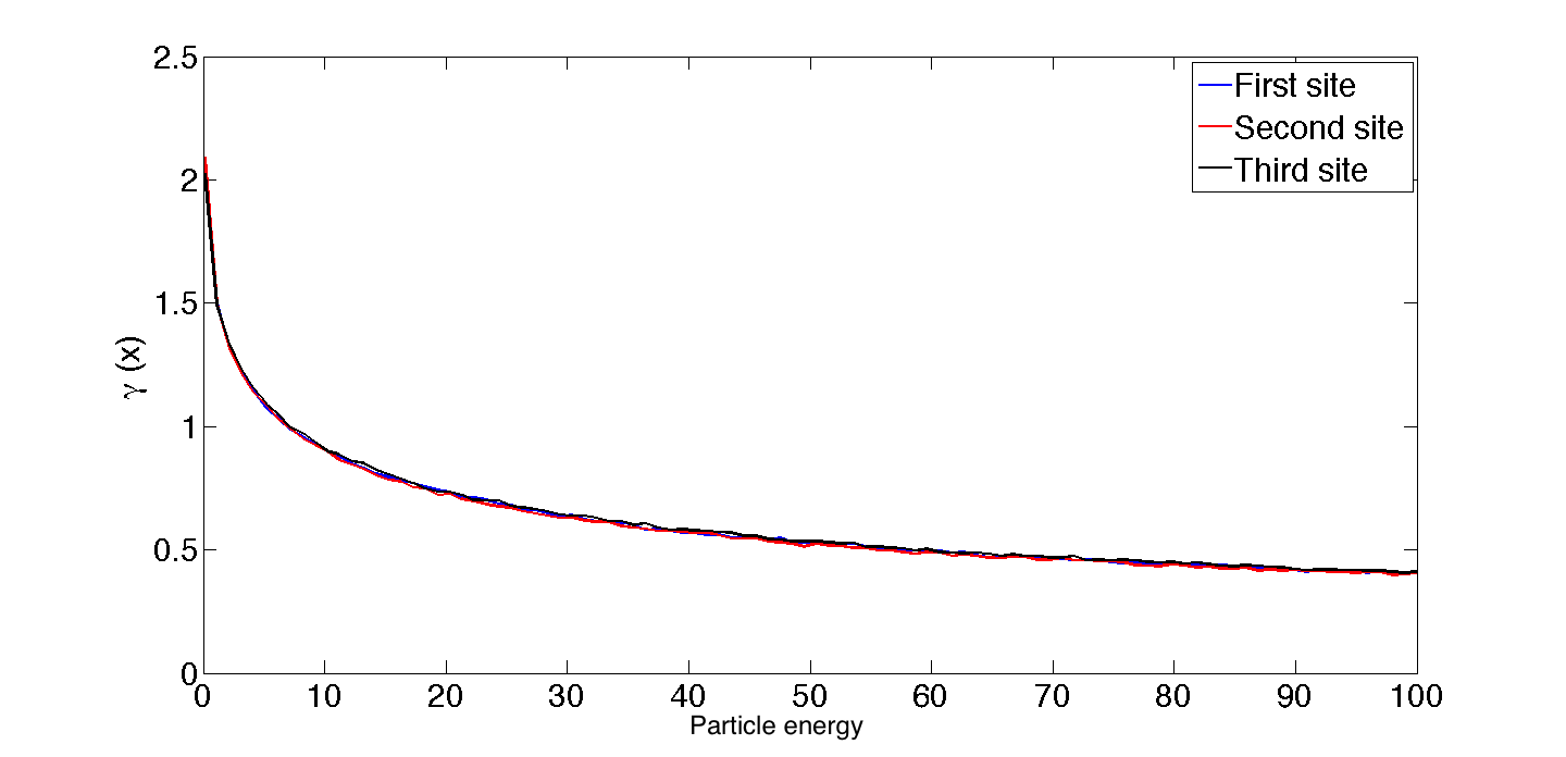
Figure 11. Change of $\gamma(\omega)$ for varying $\omega$ when particle energy at only one site changes. The energy configuration of an unchanged site is: site energy $=1$, two particles per site with particle energy = $1$. Sample size = $1\times 10^{7}$ for each initial condition.

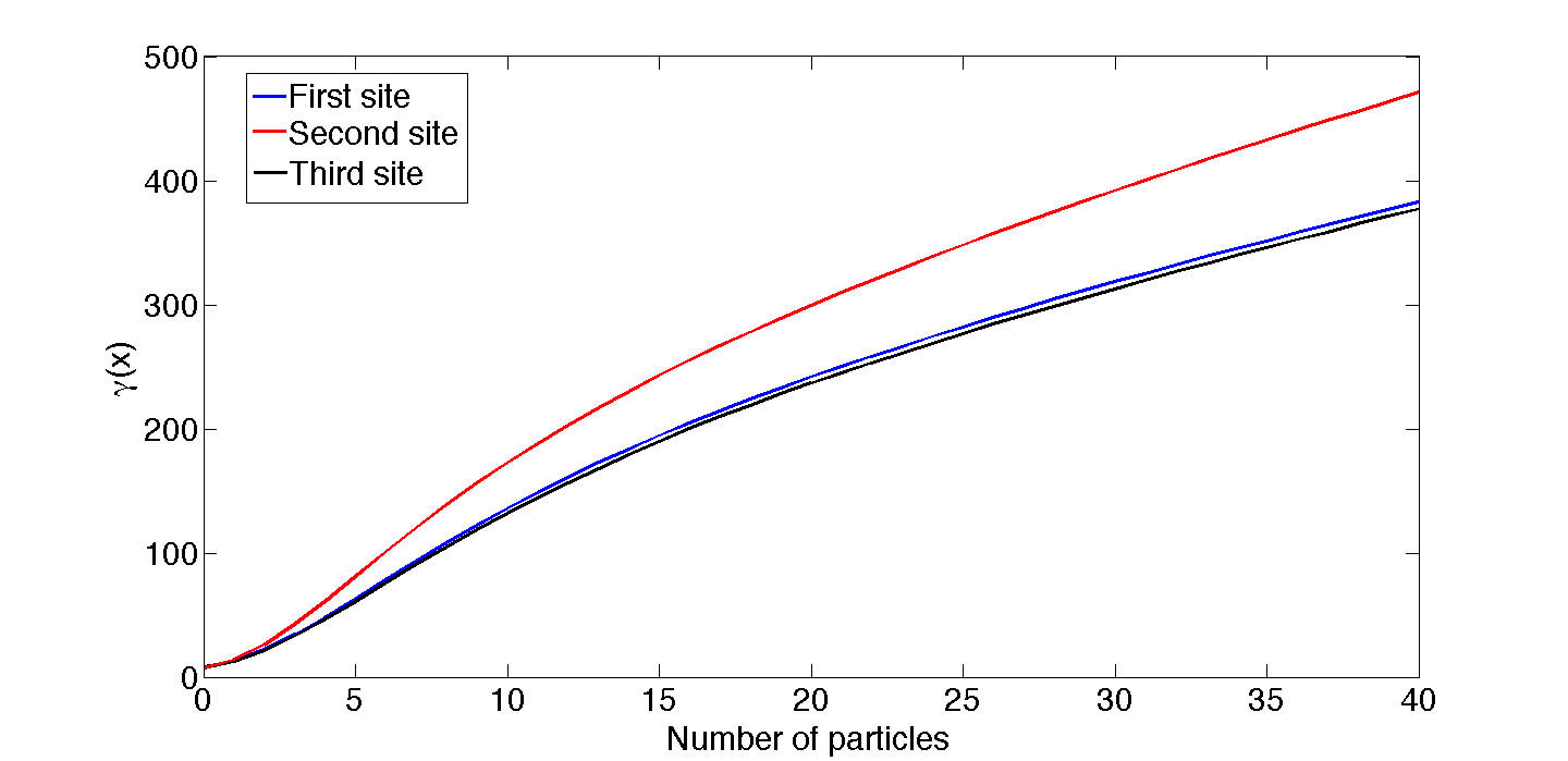
Figure 12. Change of $\gamma(\omega)$ for varying $\omega$ when number of particles at only one site changes. Energy of each particle is $0.1$. The energy configuration of an unchanged site is: site energy $=1$, two particles per site with particle energy = $1$. Sample size = $1\times 10^{7}$ for each initial condition.

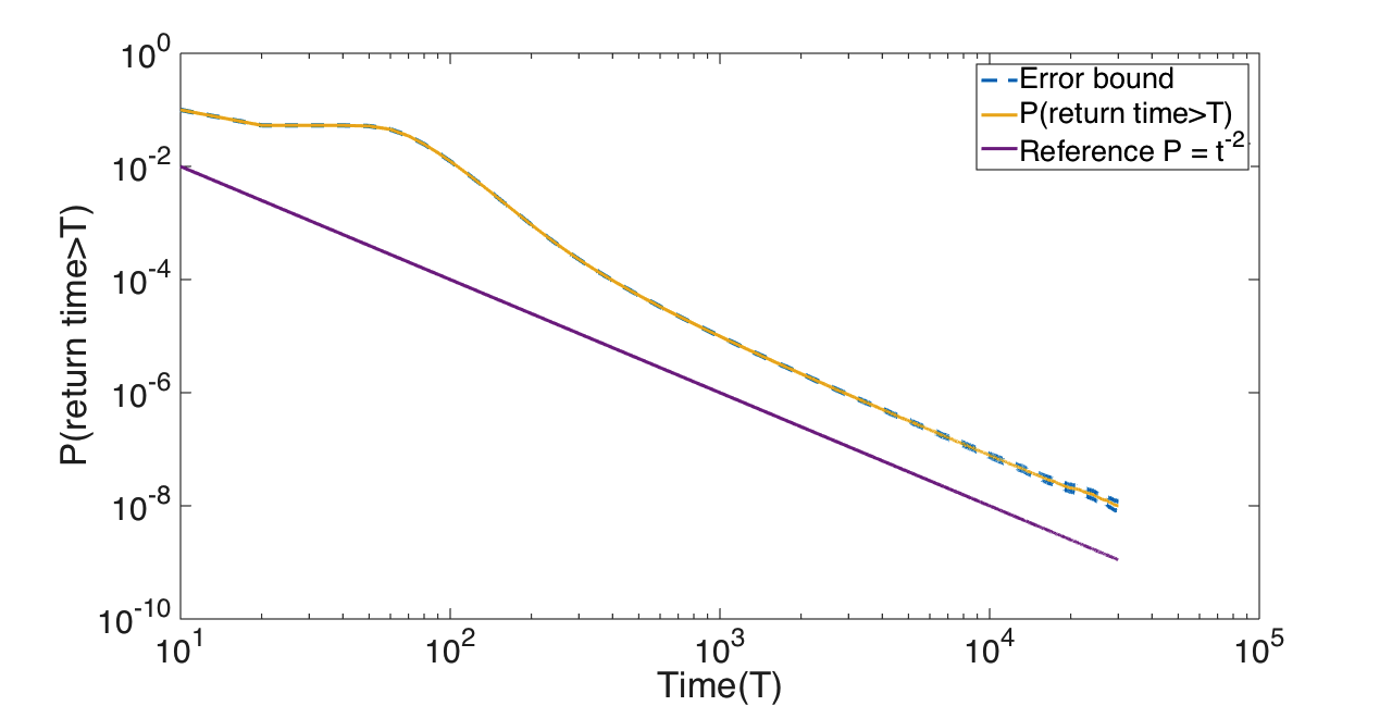
Figure 13. $\mathbb{P}_{\omega*}[\tau_{\mathfrak{C}}>t]$ for $\omega_{*}=\{(0,\{0.1,\ldots,0.1\}),\ldots,(0,\{0.1,\ldots,0.1\})\}$, for $k_{i}=40,i=1\sim 3$. Sample size = $1\times 10^{10}$. The purple line is a reference line with slope $-2$. The error bar is calculated as in Remark 3.5.

6.6. Main Conclusion

The previous subsection verifies (N1) for $\delta_{\omega_{0}}$ and $\hat{\pi}$, as well as (N2). The slopes of $\mathbb{P}[\tau_{\mathfrak{C}}>t]$ for both initial conditions are $2$. Note that $\mathbb{P}[\Psi_{t}=\Psi_{0}\,|\,\Psi_{0}\in K]=\mathbb{P}_{\Psi_{0}}[\mbox{ no clock rings up to }t]$ is uniformly positive for each given $t>0$. By Theorem 4.5, (N1) and (N2) hold for $\omega_{n}$ with parameter $2-\epsilon/2$ for arbitrarily small $\epsilon>0$. Therefore, conclusions (a)-(d) in Section 4.4 hold for $\omega_{n}$.

It remains to pass the results for $\omega_{n}$ to $\omega_{t}$. By Proposition 4.3, it is sufficient to prove “continuity at zero” for $\omega_{t}$.

Lemma 6.5.

For any probability measure $\mu$ on $\Omega$,

$$\lim_{\delta\rightarrow 0}\|\mu P^{\delta}-\mu\|_{TV}=0$$

Proof.

It is sufficient to prove that for any $\varepsilon>0$, there exists a $\delta>0$ such that

$$\|\mu P^{\delta}-\mu\|_{TV}\leq\epsilon\,.$$

Since $\mu$ is finite, there exists a bounded set $A\subset\Omega:=\{0\leq k_{i}\leq K,0\leq s_{i}\leq S,0\leq x_{j}^{i}\leq M\}$ such that $\mu(A)>1-\epsilon/4$. By the definition of $A$, clock rates for initial values in $A$ are uniformly bounded. Therefore, one can find a sufficiently small $\delta>0$, such that $\mathbb{P}[\mbox{ no clock rings on }[0,\delta)]\geq 1-\epsilon/4$. For any set $U\subset\Omega$, the same calculation as in the proof of Lemma 5.6 implies

$$|(\mu P^{\delta})(U)-\mu(U)|<\epsilon$$

for any $U\subset\Omega$. By the definition of the total variation norm, we have

$$\|\mu P^{\delta}-\mu\|\leq\epsilon\,.$$

This completes the proof.

∎

It remains to prove the uniqueness of the invariant measure.

Proposition 6.6.

For any $h>0$, $\omega^{h}_{n}$ admits at most one invariant probability measure.

Proof.

This proof is the same as that of Proposition 5.7. ∎

In summary, we have the following conclusions for $\omega_{t}$.

1. For any $T_{L}$, T_R, there exists a unique invariant probability measure $\pi$, i.e., the nonequilibrium steady-state, which is absolutely continuous with respect to the reference measure on $\Omega$.

2. For almost every $\omega_{0}\in\Omega$ and any sufficiently small $\varepsilon>0$, we have

   $$\lim_{t\rightarrow\infty}t^{2-\varepsilon}\|\delta_{\omega_{0}}P^{t}-\hat{\pi}P^{t}\|_{TV}=0\,.$$

3. For any functions $\eta$, $\xi\in L^{\infty}(\Omega)$, we have

   $$C_{\pi}^{\eta,\xi}(t)\leq O(1)\cdot t^{\varepsilon-2}$$

   for any $\varepsilon>0$.

References

- [1] Alan Agresti and Brent A Coull. Approximate is better than “exact” for interval estimation of binomial proportions. The American Statistician, 52(2):119–126, 1998.
- [2] Edward J Anderson and Michael C Ferris. A direct search algorithm for optimization with noisy function evaluations. SIAM Journal on optimization, 11(3):837–857, 2001.
- [3] Krishna B Athreya, Hani Doss, Jayaram Sethuraman, et al. On the convergence of the markov chain simulation method. The Annals of Statistics, 24(1):69–100, 1996.
- [4] Federico Bonetto, Joel L Lebowitz, and Luc Rey-Bellet. Fourier’s law: a challenge to theorists. Mathematical physics, 2000:128–150, 2000.
- [5] Jean Bricmont and Antti Kupiainen. Towards a derivation of fourier? s law for coupled anharmonic oscillators. Communications in mathematical physics, 274(3):555–626, 2007.
- [6] Leonid Bunimovich, Carlangelo Liverani, Alessandro Pellegrinotti, and Yurii Suhov. Ergodic systems of n balls in a billiard table. Communications in mathematical physics, 146(2):357–396, 1992.
- [7] Andrew R Conn, Katya Scheinberg, and Luis N Vicente. Introduction to derivative-free optimization. SIAM, 2009.
- [8] Mary Kathryn Cowles and Jeffrey S Rosenthal. A simulation approach to convergence rates for markov chain monte carlo algorithms. Statistics and Computing, 8(2):115–124, 1998.
- [9] Noé Cuneo and J-P Eckmann. Non-equilibrium steady states for chains of four rotors. Communications in Mathematical Physics, pages 1–37, 2016.
- [10] Noé Cuneo, Jean-Pierre Eckmann, and Christophe Poquet. Non-equilibrium steady state and subgeometric ergodicity for a chain of three coupled rotors. Nonlinearity, 28(7):2397, 2015.
- [11] B Derrida, JL Lebowitz, and ER Speer. Large deviation of the density profile in the steady state of the open symmetric simple exclusion process. Journal of statistical physics, 107(3-4):599–634, 2002.
- [12] Randal Douc, Gersende Fort, Eric Moulines, and Philippe Soulier. Practical drift conditions for subgeometric rates of convergence. Annals of Applied Probability, pages 1353–1377, 2004.
- [13] J-P Eckmann, C-A Pillet, and Luc Rey-Bellet. Non-equilibrium statistical mechanics of anharmonic chains coupled to two heat baths at different temperatures. Communications in Mathematical Physics, 201(3):657–697, 1999.
- [14] J-P Eckmann and L-S Young. Nonequilibrium energy profiles for a class of 1-d models. Communications in Mathematical Physics, 262(1):237–267, 2006.
- [15] Brandon Franzke and Bart Kosko. Noise can speed convergence in markov chains. Physical Review E, 84(4):041112, 2011.
- [16] Pierre Gaspard and Thomas Gilbert. Heat conduction and fourier’s law by consecutive local mixing and thermalization. Physical review letters, 101(2):020601, 2008.
- [17] Alexander Grigo, Konstantin Khanin, and Domokos Szasz. Mixing rates of particle systems with energy exchange. Nonlinearity, 25(8):2349, 2012.
- [18] Martin Hairer. Convergence of markov processes. lecture notes, 2010.
- [19] Martin Hairer. On malliavinʼs proof of hörmanderʼs theorem. Bulletin des sciences mathematiques, 135(6-7):650–666, 2011.
- [20] Martin Hairer and Jonathan C Mattingly. Spectral gaps in wasserstein distances and the 2d stochastic navier-stokes equations. The Annals of Probability, pages 2050–2091, 2008.
- [21] Martin Hairer and Jonathan C Mattingly. Slow energy dissipation in anharmonic oscillator chains. Communications on Pure and Applied Mathematics, 62(8):999–1032, 2009.
- [22] Martin Hairer and Jonathan C Mattingly. Yet another look at harris’ ergodic theorem for markov chains. In Seminar on Stochastic Analysis, Random Fields and Applications VI, pages 109–117. Springer, 2011.
- [23] Martin Hairer, Jonathan C Mattingly, and Michael Scheutzow. Asymptotic coupling and a general form of harris’ theorem with applications to stochastic delay equations. Probability Theory and Related Fields, 149(1):223–259, 2011.
- [24] David P Herzog and Jonathan C Mattingly. A practical criterion for positivity of transition densities. Nonlinearity, 28(8):2823, 2015.
- [25] Lars Hörmander. Hypoelliptic second order differential equations. Acta Mathematica, 119(1):147–171, 1967.
- [26] Søren F Jarner, Gareth O Roberts, et al. Polynomial convergence rates of markov chains. The Annals of Applied Probability, 12(1):224–247, 2002.
- [27] Galin L Jones and James P Hobert. Sufficient burn-in for gibbs samplers for a hierarchical random effects model. Annals of statistics, pages 784–817, 2004.
- [28] C Kipnis, C Marchioro, and E Presutti. Heat flow in an exactly solvable model. Journal of Statistical Physics, 27(1):65–74, 1982.
- [29] Yao Li. On the stochastic behaviors of locally confined particle systems. Chaos: An Interdisciplinary Journal of Nonlinear Science, 25(7):073121, 2015.
- [30] Yao Li. On the polynomial convergence rate to nonequilibrium steady-states. arXiv preprint arXiv:1607.08492, 2016.
- [31] Yao Li and Lai-Sang Young. Nonequilibrium steady states for a class of particle systems. Nonlinearity, 27(3):607, 2014.
- [32] Yao Li and Lai-Sang Young. Polynomial convergence to equilibrium for a system of interacting particles. Annals of Appiled Probability, accepted.
- [33] Torgny Lindvall. On coupling of discrete renewal processes. Probability Theory and Related Fields, 48(1):57–70, 1979.
- [34] Torgny Lindvall. Lectures on the coupling method. Courier Dover Publications, 2002.
- [35] Paul Malliavin. Stochastic calculus of variation and hypoelliptic operators. In Proc. Intern. Symp. SDE Kyoto 1976, pages 195–263. Kinokuniya, 1978.
- [36] Kerrie L Mengersen, Richard L Tweedie, et al. Rates of convergence of the hastings and metropolis algorithms. The Annals of Statistics, 24(1):101–121, 1996.
- [37] Sean P Meyn and Richard L Tweedie. Stability of markovian processes ii: Continuous-time processes and sampled chains. Advances in Applied Probability, 25(03):487–517, 1993.
- [38] Sean P Meyn and Richard L Tweedie. Stability of markovian processes iii: Foster-lyapunov criteria for continuous-time processes. Advances in Applied Probability, pages 518–548, 1993.
- [39] Sean P Meyn and Richard L Tweedie. Markov chains and stochastic stability. Cambridge University Press, 2009.
- [40] Esa Nummelin. A splitting technique for harris recurrent markov chains. Zeitschrift für Wahrscheinlichkeitstheorie und verwandte Gebiete, 43(4):309–318, 1978.
- [41] Esa Nummelin and Pekka Tuominen. Geometric ergodicity of harris recurrent marcov chains with applications to renewal theory. Stochastic Processes and Their Applications, 12(2):187–202, 1982.
- [42] Esa Nummelin and Pekka Tuominen. The rate of convergence in orey’s theorem for harris recurrent markov chains with applications to renewal theory. Stochastic Processes and Their Applications, 15(3):295–311, 1983.
- [43] Luc Rey-Bellet and Lawrence E Thomas. Asymptotic behavior of thermal nonequilibrium steady states for a driven chain of anharmonic oscillators. Communications in Mathematical Physics, 215(1):1–24, 2000.
- [44] Luis Miguel Rios and Nikolaos V Sahinidis. Derivative-free optimization: a review of algorithms and comparison of software implementations. Journal of Global Optimization, 56(3):1247–1293, 2013.
- [45] Hannes Risken. The fokker-planck equation. methods of solution and applications, vol. 18 of. Springer Series in Synergetics, 1989.
- [46] Gareth O Roberts, Jeffrey S Rosenthal, and Peter O Schwartz. Convergence properties of perturbed markov chains. Journal of applied probability, 35(01):1–11, 1998.
- [47] Pekka Tuominen and Richard L Tweedie. Subgeometric rates of convergence of f-ergodic markov chains. Advances in Applied Probability, pages 775–798, 1994.
- [48] S Walton, O Hassan, K Morgan, and MR Brown. Modified cuckoo search: a new gradient free optimisation algorithm. Chaos, Solitons & Fractals, 44(9):710–718, 2011.
- [49] Tatiana Yarmola. Sub-exponential mixing of open systems with particle–disk interactions. Journal of Statistical Physics, pages 1–20, 2013.
- [50] Tatiana Yarmola. Sub-exponential mixing of random billiards driven by thermostats. Nonlinearity, 26(7):1825, 2013.