Thermalization, Freeze-out and Noise: Deciphering Experimental Quantum Annealers

Abstract

By contrasting the performance of two quantum annealers operating at different temperatures, we address recent questions related to the role of temperature in these devices and their function as ‘Boltzmann samplers’. Using a method to reliably calculate the degeneracies of the energy levels of large-scale spin-glass instances, we are able to estimate the instance-dependent effective temperature from the output of annealing runs. Our results corroborate the ‘freeze-out’ picture which posits two regimes, one in which the final state corresponds to a Boltzmann distribution of the final Hamiltonian with a well-defined ‘effective temperature’ determined at a freeze-out point late in the anneal, and another regime in which such a distribution is not necessarily expected. We find that the output distributions of the annealers do not in general correspond to a classical Boltzmann distribution for the final Hamiltonian. We also find that the effective temperatures at different programming cycles fluctuate greatly, with the effect worsening with problem size. We discuss the implications of our results for the design of future quantum annealers to act as more effective Boltzmann samplers and for the programming of such annealers.

I Introduction

A handful of recent studies suggest that quantum annealers may be well suited to function as fast thermal samplers Amin (2015); M. H. Amin, E. Andriyash, J. Rolfe, B. Kulchytskyy, R. Melko (2016); Benedetti et al. (2016); Zhang et al. (2017). By taking advantage of their finite temperature nature  Katzgraber et al. (2015); V. Martin-Mayor and I. Hen (2015); Benedetti et al. (2016); Marshall et al. (2016); Zhang et al. (2017), potentially they may sample from Boltzmann distributions of certain cost functions more efficiently than can be done classically. Such a capability opens up the exciting possibility of applications of quantum annealing to so-far-uncharted avenues of research, with immediate applications to domains such as deep learning networks and restricted Boltzmann machines  Benedetti et al. (2016); Adachi and Henderson (2015); M. H. Amin, E. Andriyash, J. Rolfe, B. Kulchytskyy, R. Melko (2016).

The main mechanisms that determine the distributions from which output configurations are drawn are thus far unclear. Further insights into the role of temperature, and the capabilities of experimental quantum annealing optimizers to quickly thermalize, are challenging to obtain due to the limited ability to probe the inner workings of these machines, as well as the lack of control over most operating parameters Benedetti et al. (2016); Adachi and Henderson (2015); Zhang et al. (2017).

To circumvent these difficulties, we devised an experiment, directly comparing the performance of two commercially available quantum annealers operating at different temperatures (we shall refer to those as ‘hot’ and ‘cold’ henceforth). This key difference, together with a newly devised method to accurately calculate the degeneracies of certain large-scale spin-glass instances, offers us a unique opportunity to study the effects of temperature. Our results indicate that these instances do not in general equilibrate at Boltzmann distributions corresponding to the final classical Hamiltonian, but are significantly affected by nonzero quantum fluctuations and noise. Our results corroborate the ‘freeze-out’ picture Johnson et al. (2011); Amin (2015); M. H. Amin, E. Andriyash, J. Rolfe, B. Kulchytskyy, R. Melko (2016), which posits one regime in which the final state corresponds to a Boltzmann distribution of the final Hamiltonian with well-defined ‘effective (classical) temperature’ determined at a generally unknown freeze-out point late in the anneal, and another regime in which such a distribution would not necessarily be expected. While providing evidence for this picture, our results speak against the hypothesis that most instances fall in the first regime.

We find that these effective temperatures fluctuate greatly at different programming cycles, with the effect worsening with problem size. We discuss factors potentially contributing to this adverse effect, including so-called $J$-chaos in which control errors and other sources of noise mean that the problem run on the machine is different from the one programmed in. We discuss the implications of our results for the design of future quantum annealers to act as efficient Boltzmann samplers and for the programming of such annealers.

I.1 Quantum annealing and quantum annealers

Standard transverse field quantum annealing works by evolving the system over rescaled time $s=t/\mathcal{T}\in[0,1]$ where $t$ is time and $\mathcal{T}$ is the overall runtime of the annealing process. The total Hamiltonian of the system is given by

$$H(s)=A(s)H_{d}+B(s)H_{p}\,,$$ (1)

where $H_{p}=\sum_{\langle i,j\rangle}J_{ij}\sigma_{i}^{z}\sigma_{j}^{z}+\sum_{i}h_{i}\sigma_{i}^{z}$ is the programmable Ising spin-glass problem (the final Hamiltonian) to be sampled defined by the parameters $\{J_{ij},h_{i}\}$, and $H_{d}=-\sum_{i}\sigma^{x}_{i}$ is a transverse-field Hamiltonian which provides the quantum fluctuations (the initial Hamiltonian). We identify two dimensionless scales associated with the annealing, namely, the one associated with quantum fluctuations $Q(s)=A(s)/B(s)$ and the scale associated with thermal fluctuations $k_{B}T/B(s)$, both of which are shown in Fig. 1 for both the ‘hot’ and ‘cold’ processors.

Current quantum annealers suffer from intrinsic control errors (ICE) King and McGeoch (2014); V. Martin-Mayor and I. Hen (2015) such as imperfect digital-to-analog conversion when programming the problem parameters onto the machine, and $1/f$-noise whose effect is parameter changes even within a single programming cycle (a consecutive batch of anneals run on the machine) Zhu et al. (2016); Boixo et al. (2016). For both contrasted quantum annealers, these random errors may be approximated as normally distributed according to $\sim\mathcal{N}(0,0.05J)$ [resp. $\sim\mathcal{N}(0,0.03h)$] where $J$ (resp. $h$) is the maximal value over all the programmed $J_{ij}$ (resp. $h_{i}$). Some problems have resilience to such errors Katzgraber et al. (2015); Venturelli et al. (2015), whereas others are susceptible to a phenomenon referred to as $J$-chaos, in which output ‘solutions’ correspond to the wrong, or malformed, problem, generally reducing the success probability Nifle and Hilhorst (1992); Ney-Nifle (1998); Krzakala and Bouchaud (2005); Katzgraber and Krzakala (2007); Venturelli et al. (2015); V. Martin-Mayor and I. Hen (2015).

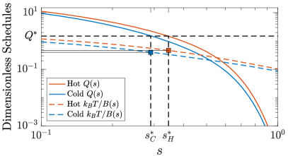
Figure 1: Dimensionless annealing schedules and temperatures of the hot and cold DW2 processors. We plot quantum fluctuations $Q(s)$, and thermal fluctuations $k_{B}T/B(s)$, as a function of rescaled annealing time, $s$, for each machine. An example of freeze-out is shown; the distribution approximately halts at some fixed, instance-dependent value of $Q^{*}:=Q(s^{*})$ (dashed black line) which corresponds to a freeze-out point $s^{*}$ (denoted $s_{C}^{*},s_{H}^{*}$) and dimensionless effective temperature $k_{B}T/B(s^{*})$ (squares), for each machine. The solid black lines illustrate that freeze-out may correspond to different effective temperatures.

I.2 Freeze-out conjecture

If problems thermalized instantly, quantum annealers would return configurations sampled from a Boltzmann distribution, in which each configuration $c$ has weight proportional to $e^{-\beta^{\text{eff}}_{\text{ideal}}E_{c}}$, where $E_{c}$ is the configuration’s classical cost (under $H_{p}$) and $\beta^{\text{eff}}_{\text{ideal}}\equiv B(1)/k_{B}T$ is an effective dimensionless inverse temperature, with $T$ being the operating temperature of the machine Albash et al. (2017). It is known, however, that effective inverse-temperatures $\beta^{\text{eff}}$ extracted from experimentally sampled distributions are usually lower than $\beta^{\text{eff}}_{\text{ideal}}$, and that the observed inverse-temperatures differ across problem instances Amin (2015); M. H. Amin, E. Andriyash, J. Rolfe, B. Kulchytskyy, R. Melko (2016); Benedetti et al. (2016).

The freeze-out conjecture Johnson et al. (2011); Amin (2015); M. H. Amin, E. Andriyash, J. Rolfe, B. Kulchytskyy, R. Melko (2016) explains these high observed effective temperatures by positing a “small $Q$ regime” in which the evolution is quasi-static, returning a final population that is close to a Boltzmann distribution of $H_{p}$ with a well-defined effective temperature, and a regime in which the final population would not necessarily be of this form. In the first regime, the final distribution is determined by a ‘freezing’ of the evolution (after which no dynamics occur) at an unknown, instance-dependent, but physical-temperature independent, ‘freeze-out’ point $s^{*}$ where thermal fluctuations, whose strength is coupled to the quantum fluctuations $Q(s^{*})$ driving the system, become negligibly small .

As illustrated in Fig. 1, the freeze-out point is conjectured to happen at a temperature-independent (but instance-dependent) value $s^{*}$ Amin (2015). Only when $Q(s^{*})$ at the freeze-out is small is the final distribution expected to be a classical Boltzmann distribution for $H_{p}$ with (dimensionless) effective temperature $\beta^{\text{eff}}=B(s^{*})/k_{B}T$; otherwise, the resultant distribution will generally not correspond to an equilibration at any given point, but may instead result from different parts of the system equilibrating at different temperatures and times Amin (2015).

I.3 High-level approach

We proceed by taking as a working hypothesis that most instances have a well-defined freeze-out point in the range $A(s)\ll B(s)$. We work through the implications of this hypothesis, and demonstrate empirically that it does not hold for the majority of instances. We do so by estimating a freeze-out point from the data for each instance, and then checking whether or not that point falls in the $A(s)\ll B(s)$ regime. Most instances fail this consistency check. Outside of that regime, the freeze-out conjecture does not predict a well-defined freeze-out point; different parts of the system may freeze at different times, and even if an instance does have a well-defined freeze-out point outside $A(s)\ll B(s)$, the distribution would have a strong quantum component (from $H_{d}$), so would be a distribution of quantum states, and not of the form $e^{-\beta^{\text{eff}}H_{p}}$. These results are consistent with the freeze-out conjecture, but not with the hypothesis that most instances fall within the freeze-out regime that yields a classical Boltzmann distribution.

II Experiment and methods

We make use of two $512$-qubit D-Wave Two (DW2) quantum annealers . The mean temperatures of the ‘hot’ and ‘cold’ machines were about 16.0 mK and 13.2 mK, respectively (further details are provided in Appendix A).

We designed $1300$ random spin-glass instances of the planted-solution type Hen et al. (2015) for each of seven different problem sizes corresponding to $L\times L$ grids of $8$-qubit cells of the hardware DW2 Chimera graph with $L=2\ldots 8$ (see Fig. 2). We generated these instances as per Ref. Hen et al. (2015) (the reader is referred to Appendix B for more details). This class of instances is particularly suitable for our purposes for two main reasons: i) the ground state energies of the generated problems are known in advance, and ii) the exact degeneracies of the ground and first excited states are computable Zhang et al. (2017). These two facts allow us to, with high accuracy and confidence, measure $\beta^{\text{eff}}$, as will be explained below. We generated instances on the intersection of the two hardware graphs ($501$ qubits) in order to avoid biases associated with malfunctioning qubits on either machine (as shown in Fig. 2).

To gather our statistics, each instance was run 440,000 times over 22 ‘programming cycles’ on each machine, with anneal times in range [20-40] $\mu$s. A programming cycle consists of running the same instance sequentially on a single machine up to (as chosen by the user) 20,000 times, from which statistics are returned; from each programming cycle we obtained the ground state success probability (how often the ground state of the problem was found). We use this data to estimate $\beta^{\text{eff}}$.

Figure 2: Intersected Chimera. Intersection of the two D-Wave Chimera graphs, with 501 operating qubits. Red disks denote non-operational qubits on one (or both) of the two machines. We denote the size of a square subgraph by an integer $L\leq 8$.

To evaluate $\beta^{\text{eff}}$ we employ two independent, complementary, techniques, which together allow us to estimate with high accuracy and confidence the degeneracies of the energy levels of the problem instances. The first, the well-known Wang-Landau (WL) entropic sampler Wang and Landau (2001), statistically estimates the degeneracy of the energy levels (see Appendix C for technical details). Since the WL algorithm is prone to statistical errors as well as false convergences, we employ in parallel a newly-devised algorithm that uses the feature that planted-solution instances can be written as a sum of local terms Zhang et al. (2017). The algorithm computes the degeneracies of the ground and first excited states exactly. When the WL estimate is outside $\pm 5\%$ of the exact value for either the ground or first excited state, we discard this instance as we know it has not converged properly. The combination of these two algorithms allows for the faithful estimation of the degeneracies. We show in Fig. 3 an example of a successful implementation of these two algorithms, where the Wang-Landau ground and first excited estimates are within 5% error of the exact values.

The above procedure yielded some 2200 instances in total, for problem sizes up to 282 qubits, for which we were able to accurately calculate the degeneracies. The difficulty in obtaining an accurate measurement, especially for the larger problems, was due mainly to i) the D-Wave machine not being able to solve many of the ‘hard’ problems, ii) there were too many degenerate states for the exact counter to enumerate (exceeded our chosen cut-off value of $10^{7}$ ground states, which become prohibitively expensive to compute), or iii) Wang-Landau estimate deviated too far from exact counter results (generally from under-sampling the low energy states).

Armed with these degeneracies, we estimate the inverse-temperature $\beta^{\text{eff}}$ for each instance by minimizing the distance between the observed ground state success probability $P_{0}$ and the predicted one (i.e., the conjectured Boltzmann distribution):

$$\left|P_{0}-\left(\sum_{k=0}\frac{g_{k}}{g_{0}}e^{-\beta^{\text{eff}}(E_{k}-E_{0})}\right)^{-1}\right|\,.$$ (2)

Here, $\{g_{k},E_{k}\}$ are the degeneracy and energy of the $k$-th level, respectively. The total number of instances for which $\beta^{\text{eff}}$ was successfully estimated, for each problem size $L=2\dots 8$, is [664,745,449,266,38,0,0].

Figure 3: Degeneracy counting. Main figure: The degeneracies of the first five energy levels of two of the $282$-qubit problem instances as found by the Wang-Landau algorithm (error bars represent 95% confidence interval). The WL degeneracies of the first two levels lie on top of the computable exact values (solid circles). Inset: Degeneracies of all levels as a function of energy, for the same instances, as obtained by the WL algorithm.

III Results and Analysis

III.1 Thermalization

Figure 4 (top) plots the median inverse temperature $\beta^{\text{eff}}$ for each instance and machine. Error bars indicate the maximum and minimum value of $\beta^{\text{eff}}$ over all programming cycles. Evident is the overall strong linear correlation between the (inverse) effective temperatures of the two machines (Pearson coefficient 0.94). Most instances fall within, or near, the ‘thermal range’ (see caption) predicted by the ratio of physical temperatures of the machines [see yellow band in Fig. 4 (top)], illustrating the key functional role of temperature in the success probability of these problems. If the instances were thermalizing at the end of the anneal, however, we would expect to observe $\beta^{\text{eff}}_{\text{ideal}}$ of 9.7 and 11.7 (shown in Fig. 4) for the hot and cold machines, respectively. Instead, the values we observe are well below this mark: $\beta^{\text{eff}}\in[2,7]$. Thus, we are finding effective temperatures up to six times higher than would be expected from a simple thermalization picture. Moreover, the median ratio of $\beta^{\text{eff}}$ for the two machines, $R_{\beta}=1.11\pm 0.05$ (95% confidence interval) , is well below the ratio of the physical temperatures, $R_{\beta}^{\text{ideal}}=1.21\pm 0.02$ indicating an effective average temperature ratio of about $92\%$ of the ‘thermal’ ratio of $s=1$. We now examine the extent to which the freeze-out picture can explain these discrepancies.

Figure 4: Top: Effective inverse temperatures. Comparison of effective inverse temperatures on the set of instances for both the hot processor, $\beta^{\text{eff}}_{H}$, and the cold processor, $\beta^{\text{eff}}_{C}$. Error bars represent the highest and lowest values found over all programming cycles. The yellow band represents the range of physical temperature fluctuations between the devices, given by the linear relationship $y=R_{\beta}^{\mathrm{ideal}}x$ (defined in main text). The blue diamond represents $\beta^{\text{eff}}$ were (classical) thermalization to take place at the end of the anneal. Different problem sizes have different colors (see legend). Bottom: Quantum fluctuations at freeze-out. Scatter plot of the extracted $Q^{*}:=Q(s^{*})$ strengths (blue) for each instance. Ideally, both machines would yield the same value for each instance (red $y=x$ line). Median ratio is $R^{\text{small}}_{Q}=1.01$ for small $Q(s^{*})$ values (within the green square). The outputs are strongly correlated (Pearson coefficient 0.92). Error bars represent the range of $Q^{*}$ over all programming cycles.

III.2 Freeze-out

While the freeze-out point for each instance is unknown, its temperature independence means the estimates for the freeze out point should be the same whether from the cold machine or hot machine data. Using the estimated $\beta^{\text{eff}}=B(s^{*})/k_{B}T$, from which we can obtain a freeze-out point $s^{*}$ given the known operating temperatures and annealing schedules, we directly calculate $Q(s^{*})$. We then check whether the freeze-out point for each instance is the same for the two machines. We plot $Q(s^{*})$ for each instance in Fig. 4 (bottom). For instances with small $Q$ (we take $Q<10^{-1}$), we find excellent correspondence between the two machines, with an average ratio of $R^{\text{small}}_{Q}=1.01\pm 0.06$ (95% confidence interval), in agreement with the freeze-out picture, suggesting a meaningful $\beta^{\text{eff}}$, which implies final classical Boltzmann distributions, in this regime. Only a small fraction of the instances, however, correspond to a negligible $Q(s^{*})$.

For the majority of instances, $Q(s^{*})>1$, and thus contradicts our working hypothesis that most instances fall in the regime in which one would expect a well-defined freeze-out point and a final classical Boltzmann distribution. working assumption that the instances thermalize according to $H_{p}$. The ratio $R_{Q}$ over the the entire data set is $R_{Q}\approx 1.20$, substantially higher than the ‘ideal’ $R_{Q}=1$. Compared to the rest of the instances, the small $Q(s^{*})$ problems are typically easier to solve and are disproportionately smaller in problem size (see e.g. Fig. 16 in Appendix D). The freeze-out picture can also explain the lower-than-ideal effective inverse-temperature ratio $R_{\beta}=1.11$ (and higher $R_{Q}\approx 1.20$). The existence of significant quantum fluctuations outside $A(s)\ll B(s)$ leads to an overestimation of thermal fluctuations in both machines, i.e., to higher effective temperatures, as we indeed observe.

III.3 High variability in inverse temperature estimates

The magnitude of the error bars on the effective inverse temperatures per instance shown in Fig. 4 (top) reflect the large fluctuations in success probabilities between programming cycles. We discuss various factors that contribute to that variance.

It is known that the location of the freeze-out point (and hence the success probability) has a weak logarithmic dependence on the annealing time Amin (2015); V. Martin-Mayor and I. Hen (2015), with longer anneal times having later freeze-out points because there is more time for fluctuations to take place. We indeed find such an effect (see Figs. 11, 12 of Appendix D), though our results show that this typically accounts for less than a 1$\%$ variability between different anneal times and therefore does not explain the spread we observe. If the variation were due purely to statistical variations from cycle to cycle, one would expect statistical fluctuations in success probability $P_{0}$ on the order of $\delta P_{0}=\sqrt{P_{0}(1-P_{0})/N_{\text{anneals}}}$. Fig. 5 (top) shows $R_{\Delta/\delta}=\Delta P_{0}/\delta P_{0}$, the ratio of typical magnitude of actual fluctuations in success probabilities $\Delta P_{0}$ to the expected magnitude of purely statistical fluctuations $\delta P_{0}$. We find that only around 20$\%$ of the instances exhibit fluctuations of success probability $R_{\Delta/\delta}$ below 1. For most instances, typical fluctuations are about an order of magnitude greater than statistical fluctuations, with some fluctuations being considerably greater. We attribute these large ratios, to $J$-chaos V. Martin-Mayor and I. Hen (2015) from ICE and other noise, which affect the local fields and coupling parameters within and between cycles. Noise unrelated to programming parameters may also play a role.

Figure 5 (bottom) shows, as a function of problem size, the average variation in $\beta^{\text{eff}}$, as measured by the ratio of the 95th to 5th percentile values found over all programming cycles. The larger the problem size, the greater the size of the fluctuations. This trend is expected as larger problems, with more couplings, have more potential to be adversely affected by control errors, and other sources of noise . It is critical to understand why these fluctuations scale with problem size, and their root cause, so as to devise strategies to keep these errors from becoming unmanageable as chip sizes increase. For a fixed problem size, we do not observe a clear correlation between success probability and the variance in the $\beta^{\text{eff}}$ estimates (Fig. 6), providing evidence that the fluctuations we observe in Fig. 5 (bottom) are indeed due to differences in problem size and not problem difficulty (though of course the two are related) .

Figure 5: Top: Ratio of magnitude of actual fluctuations in success probabilities to magnitude of statistical fluctuations, $R_{\Delta/\delta}$, for the various instances on the hot and cold processors. For most instances, the fluctuations in success probabilities over programming cycles is far greater (by an order of magnitude) than what one might expect from fluctuations of a purely statistical nature. Bottom: Typical spread of effective inverse temperature as a function of problem size. Our measure for spread is the $95$th to $5$th percentile mean ratio of $\beta^{\text{eff}}$ averaged over instances of each problem size. We take the ratio to overcome any bias from the cold chip recording higher values of $\beta^{\text{eff}}$ (see inset). We find both devices follow a nearly identical trend: fluctuations increase and $\beta^{\text{eff}}$ decreases with problem size. Inset: Median $\beta^{\text{eff}}$ for each problem size. 95% confidence interval error bars obtained by bootstrapping over the instances of each particular $N$.

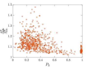
Figure 6: Variance with success probability. Spread of effective inverse temperature as a function of success probability, as determined by the $95$th to 5th percentile ratio of $\beta^{\text{eff}}$ over all programming cycles, for $N=70$ (we pick this problem size as it is the one for which we have the most number of instances with reliable data). Data from the hot machine.

IV Conclusions

By conducting parallel experiments on two quantum annealers, each operating at a different temperature, we studied key mechanisms determining their output distributions. In particular, we tested the freeze-out conjecture Johnson et al. (2011); Amin (2015); M. H. Amin, E. Andriyash, J. Rolfe, B. Kulchytskyy, R. Melko (2016) by comparing the performance of the two machines on certain Ising problems, making use of a recent method to accurately estimate the degeneracies of such problems. With a working hypothesis that the output distribution is indeed a Boltzmann distribution of the classical problem Hamiltonian, we calculated the effective inverse temperatures for each instance and machine, $\beta^{\text{eff}}$, from which we calculated the freeze-out point.

For instances which our results show exhibit negligible quantum fluctuations (small $Q$), we find a well defined temperature-independent (i.e., machine-independent) freeze-out point, in agreement with the prediction of the freeze-out hypothesis for the small $Q$ regime. This agreement suggests for these instances the output distribution is indeed a classical Boltzmann distribution for $H_{p}$, with well defined effective temperature.

Our results also show, however, that for the majority of instances, the estimated freeze-out point is not in the regime of negligible quantum fluctuations, and therefore does not have a well-defined effective temperature, nor is there any reason to believe the output should follow a classical Boltzmann distribution.

Moreover, we also observed that the effective temperatures at different programming cycles can wildly fluctuate. Our data indicates that this effect worsens with larger problem size. These observations show that for future quantum annealers to be effective as Boltzmann samplers, designers must take into account these results, and find ways to ensure that instances thermalize in the $A(s)\ll B(s)$ regime, and such that the effective temperatures are more stable. Moving forward, it would therefore be worthwhile to have additional estimators of temperature, and more robust ways to reconstruct the Boltzmann distribution (i.e., the one we conjecture for small $Q$) Raymond et al. (2016).

Promising directions include reducing sources of noise that contribute to intrinsic control errors (ICE) in quantum annealing hardware, and exploring alternate annealing schedules and non-standard drivers to enable more instances to equilibrate at a unique point late enough in the anneal that the quantum fluctuations are negligible. For machine learning, another approach is possible. It is not clear how accurately one needs to sample from Boltzmann distributions for machine learning, or even that Boltzmann distributions are optimal for this purpose. A tantalizing research direction is the use of distributions that have a large quantum component M. H. Amin, E. Andriyash, J. Rolfe, B. Kulchytskyy, R. Melko (2016), particularly given that certain distributions generated by quantum Hamiltonians are believed to have no efficient classical sampling mechanism Semay and Ducobu (2016); R. W. Robinett (1995). A deeper understanding of these processes will have profound implications for the design of future annealers and the prospects of utilizing quantum annealers as efficient Boltzmann samplers for machine learning and beyond.

Appendix A The Google-NASA-USRA (‘cold’) and Lockheed-Martin-USC (‘hot’) D-Wave Two processors

The quantum annealer used in our work is the D-Wave Two (DW2) device Bunyk et al. (2014). This device is designed to solve optimization problems by evolving a known initial configuration — the ground state of a transverse field $H_{d}=-\sum_{i}\sigma_{i}^{x}$, where $\sigma_{i}^{x}$ is the Pauli spin-$1/2$ matrix acting on spin $i$ — towards the ground state of a classical Ising-model Hamiltonian which serves as a cost function that encodes the problem that is to be solved:

$$H_{p}=\sum_{\langle i,j\rangle}J_{ij}\sigma_{i}^{z}\sigma_{j}^{z}+\sum_{i}h_{i}\sigma_{i}^{z}\ .$$ (3)

The variables $\{\sigma_{i}^{z}\}$ denote either classical Ising-spin variables that take values $\pm 1$ or Pauli spin-$1/2$ matrices, the $\{J_{ij}\}$ are programmable coupling parameters, and the $\{h_{i}\}$ are programmable local longitudinal fields. The $N$ spin variables are realized as superconducting flux qubits and occupy the vertices of the D-Wave ‘Chimera’ hardware graph Bunyk et al. (2014); Choi (2011). Here, $\langle i,j\rangle$ denotes summation over the edges of the graph. The union of the two D-Wave Chimera graphs is given in Fig. 2 – this is the graph all of our problem instances were defined on.

These machines evolve the full Hamiltonian via

$$H(s)=A(s)H_{d}+B(s)H_{p}\,.$$ (4)

The way in which the strength of the initial ($H_{d}$) and final ($H_{p}$) Hamiltonians evolve is given by the parameters $A(s)$ and $B(s)$, where $s=t/\mathcal{T}\in[0,1]$ is the annealing time. Here, $\mathcal{T}$ is the total annealing time, ranging between $20\mu$s and $20m$s on these devices. The annealing schedule is given in Fig. 7 for each machine.

In Fig. 8 we show the temperature log of the D-Wave chips during the time which we collected our data.

Figure 7: Annealing schedules of the USC (hot) and NASA (cold) DW2 processors. Annealing schedule [see Eq. (4)] in GHz as a function of dimensionless annealing time $s=t/\mathcal{T}$. We also plot the temperatures ($\hbar=1$) of the devices (see legend).

Figure 8: Temperature logs. Temperature log for the USC (hot) and NASA (cold) machines during the period of time we performed our experiments. The dashed black lines represent the mean of the data sets. The mean temperature of the ‘hot’ USC machine was about $T_{H}=16.0$ mK, and the mean temperature of the ‘cold’ NASA machine was about $T_{C}=13.2$ mK, with ratio $T_{H}/T_{C}\approx 1.21$. Note, the temperature data is sparse, sampled only twice per 24 hours.

Appendix B Generation of instances

For the generation of instances, we have chosen in this work to study problems constructed around ‘planted solutions’ – an idea borrowed from constraint satisfaction (SAT) problems Barthel et al. (2002); Krzakala and Zdeborová (2009). In these problems, the planted solution represents a ground state configuration of Eq. (3) that minimizes the energy and is known in advance. This knowledge circumvents the need to verify the ground state energy using exact (provable) solvers, which rapidly become too expensive computationally as the number of variables grows, and which were employed in earlier benchmarking studies Boixo et al. (2014); Rønnow et al. (2014). Moreover, these problems are known to possess different degrees of ‘tunable hardness’, achieved by adjusting the amount of frustration (see Ref. M. Mezard, G. Parisi and M.A. Virasoro (1987)) which we will use. Last, studying this type of problems allows us to devise an algorithm to find all minimizing configurations of the generated instances. Knowledge of both energy levels as their degeneracies is essential for the calculation of effective temperatures of the instances.

To generate the instances for the experiment we follow the guidelines introduced in Ref. Hen et al. (2015). We generate 13 groups of 100 instances, for each of 7 different sub-Chimera sizes with $L=2\dots 8$, see Fig. 2 (i.e., 9100 total instances). These 13 groups differ in the ratio $\alpha$ of number of clauses (or loops) to number of qubits contained in each instance. For every fixed ratio $\alpha$ the range of integer-valued $J_{ij}$’s, which we denote by $J_{\max}$ is fixed across the different problem sizes. D-Wave further rescales all coupling values such that the encoded values, $\tilde{J}\in[-1,1]$ which implies that for every fixed $\alpha$ both the range of $J$-values as well as the spacings between them is identical across different problem sizes.

Appendix C Wang-Landau entropic sampler

As explained in the main text, we employed a Wang-Landau entropic sampler to estimate the degeneracy of the energy levels for our generated planted-solution instances. This algorithm performs essentially a random walk over the energy landscape, where updates at each step in the algorithm are such that an approximately flat histogram of visited energies is produced. We follow the same methodology as originally described in Wang and Landau (2001). Our histogram was considered ‘flat’ when the lowest sampled energy level has been visited at least 80% of the mean of the entire histogram.

We performed 20 independent Wang-Landau runs, each up to $10^{9}$ steps for each of our instances. We then averaged over these 20 runs which provided our estimate of degeneracies for each instance. We then discarded any instances for which the ground or first excited state degeneracies did not match that for the exact solution counter (up to 5% error). This meant we had accurate degeneracy data for problems up to 282 qubits in size.

Appendix D Effects or lack thereof of additional experimental parameters

D.1 Success probabilities

In Fig. 9 we show the histogram of the success probabilities for the two machines, for all of the instances. We see the cold (NASA) machine clearly outperforms the hot (USC) machine–we expect, due to the colder operating temperature.

D.2 Programming cycles

In Fig. 10 we compare two different programming cycles (from different days) on the same machine, showing consistency over different runs.

D.3 Anneal times

We also study the effect of varying anneal time on success probability in Figs. 11 and 12. We see that there is only a very weak (logarithmic) dependence on anneal time, in accordance with Amin (2015); V. Martin-Mayor and I. Hen (2015), and moreover, it is seemingly not correlated with problem size.

D.4 Ratio of number of clauses to number of qubits

Fig. 13 shows that (within error bars) our computation of the inverse temperature ratio between the two machines is unaffected by changing the ratio of number of clauses (or loops) to number of qubits $\alpha$, and moreover, that the thermal ratio is well above the measured ratio (far outside of the error bars mostly).

Figure 9: Success probability. Probability of success (how often the ground state energy is correctly identified) of all instances and programming cycles on the two machines (‘hot’ USC machine $P_{H}$, and the ‘cold’ NASA machine $P_{C}$). Each point is a randomly chosen programming cycle (for the same instance on each machine). Number of qubits given by legend.

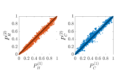
Figure 10: Machine correlation. We compare the results of two programming cycles for each instance on each machine. We see the data aligns nicely along $y=x$, albeit with sizable fluctuations (as one would expect). Compare this with Fig. 9, where data clearly deviates from $y=x$. The ‘hot’ USC machine is on the left, and the ‘cold’ NASA machine on the right.

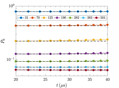
Figure 11: D-Wave success with anneal time. Average probability of success, $P_{0}$ (for the hotter USC machine), against anneal time (log scale), for different problem sizes (see legend). Each point averaged over two programming cycles, of $N_{\text{anneals}}=20,000$ anneals each. The black dash lines correspond to the value of $P_{0}$ for $t=20$ $\mu$s. One can see in general a slight increase in success probability with $t$.

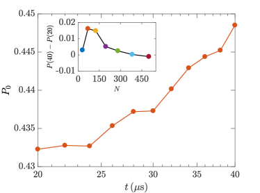
Figure 12: D-Wave success with anneal time, for single problem size. Average probability of success, $P_{0}$ (for the hotter USC machine), against anneal time (log scale), for problem size 70 ($L=3$). Note the approximate linear relationship. Inset: Difference in success probability between $t=40$ and $t=20$ $\mu$s as measured by $P(40)-P(20)$, where $P(t)$ is defined as $P_{0}$ for anneal time $t$.

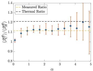
Figure 13: Effective inverse temperature ratio against clause density. As explained in the text, we generated many problems for each graph size $L=2,\dots,8$. We picked fixed and identical values of $\alpha$ (the ratio of the number of loops to the number of qubits) for each qubit size. We find that $\alpha$ has (within the 95% confidence interval error bars obtained from bootstrapping the data) mostly no effect on the effective temperature ratio we measured from our data (1.11, calculated as the median over all instances), and that it is much below the thermal ratio value of 1.21. Note the smallest $\alpha=0.1$ instances are very easy to solve ($P_{0}\approx 1$), making it hard to distinguish performance (hence temperature) differences between the machines.

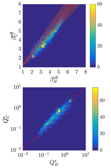
Figure 14: Density plots for $\beta^{\text{eff}}$ and $Q^{*}$. The corresponding ‘heat map’ for Fig. 2 of the main text. Color indicates the number of points in each region (given by color bar on the right hand side). Top: Red dash line is the ‘ideal’ thermal ratio (i.e. if the ratio of the effective inverse temperatures were the same as the physical ‘thermal’ inverse temperatures). The variance in physical temperature fluctuations is given by the red semi-transparent region. Bottom: Red dash line is $y=x$.

Appendix E Additional data

Relating to Fig. 4 of the main text, we produce a ‘heat map’, Fig. 14, for $\beta^{\text{eff}}$, and for $Q^{*}$ (defined in main text), for each machine, which shows the number of instances found in each small region. We notice that in the upper figure that the larger the effective inverse temperature, more instances fall within the ‘thermal region’, indicating a stronger dependence on the temperature for these instances. These instances correspond to the ones which freezeout at a later point in the anneal, and thus a smaller $Q^{*}$ in the lower figure. In this lower figure, we observe the fit is closer to the ‘ideal’ $y=x$ for smaller $Q^{*}$, and it deviates above this line for larger $Q^{*}$ (we discuss in more detail in the main text).

Also relating to Fig. 4 of the main text, we produce Figs. 15, 16, which plot $\beta^{\text{eff}}$, and $Q^{*}$, for each machine, but split up by problem size. One can see that typically the larger problems exhibit lower values of $\beta^{\text{eff}}$, and likewise, larger values of $Q^{*}$, indicating these are in fact not thermalizing according to a Boltzmann distribution.

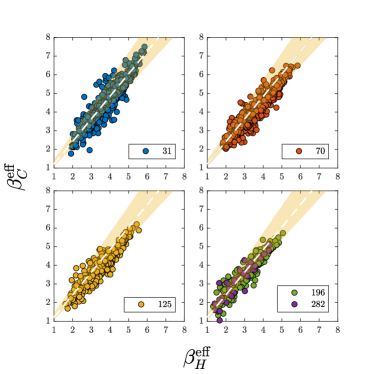
Figure 15: $\beta^{\text{eff}}$ for different problem sizes. These plots show the effective inverse temperature found by each machine (and for each instance), for the 5 different problem sizes (see legend) for which we have reliable degeneracy data. White dash line is the ‘ideal’ thermal ratio (i.e. if the ratio of the effective inverse temperatures were the same as the physical ‘thermal’ inverse temperatures). The variance in physical temperature fluctuations is given by the yellow semi-transparent region.

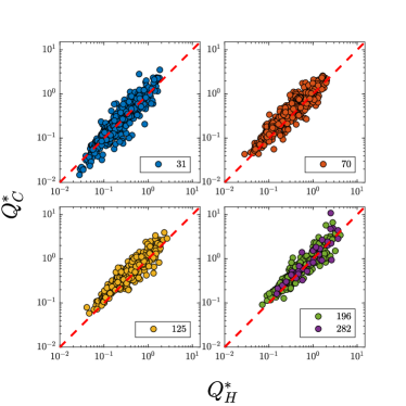
Figure 16: $Q^{*}$ for different problem sizes. These plots show the median $Q^{*}$ found by each machine (and for each instance), for the 5 different problem sizes (see legend) for which we have reliable degeneracy data. Red dash line is $y=x$.