Entanglement Complexity in Quantum Many-Body Dynamics, Thermalization and Localization

Abstract

Entanglement is usually quantified by von Neumann entropy, but its properties are much more complex than what can be expressed with a single number. We show that the three distinct dynamical phases known as thermalization, Anderson localization, and many-body localization are marked by different patterns of the spectrum of the reduced density matrix for a state evolved after a quantum quench. While the entanglement spectrum displays Poisson statistics for the case of Anderson localization, it displays universal Wigner-Dyson statistics for both the cases of many-body localization and thermalization, albeit the universal distribution is asymptotically reached within very different time scales in these two cases. We further show that the complexity of entanglement, revealed by the possibility of disentangling the state through a Metropolis-like algorithm, is signaled by whether the entanglement spectrum level spacing is Poisson or Wigner-Dyson distributed.

Introduction.— Entanglement is usually quantified by a number, the entanglement entropy, defined as the von Neumann entropy of the reduced density matrix $\rho_{A}$ of a subsystem, and it is a key concept in many different physical settings, from novel phases of quantum matter ref48 ; ref49 ; ref50 ; ref51 to cosmology bh ; susskind1 . However, there is a lot more information in the entanglement spectrum of $\rho_{A}$, namely the full set of its eigenvalues (or its logarithms) haldane-li . Recently, a measurement protocol to access the entanglement spectrum of many-body states using cold atoms has been proposed measure . The main goal of this letter is to explore the relationship between entanglement spectrum and dynamical behavior of a quantum many-body system.

In Refs. espectrum1 ; espectrum2 it was shown that the entanglement of a state generated by a quantum circuit can be simple or complex, in the sense that the state either can or cannot be disentangled by an entanglement cooling algorithm that resembles the Metropolis algorithm for finding the ground state of a Hamiltonian. The success or failure of the disentangling procedure is signaled by the so called entanglement spectrum statistics (ESS) espectrum1 ; espectrum2 , namely the distribution of the spacings between consecutive eigenvalues of $\rho_{A}$. When such a distribution is Wigner-Dyson (WD), the cooling algorithm fails. This situation occurs when the gates in the circuit are sufficient for universal computing, either classical or quantum. On the other hand, for circuits that are not capable of universal computing, the states can be disentangled and they feature a (semi-)Poisson ESS.

In this letter, we focus on systems whose dynamics is controlled by a time-independent quantum many-body Hamiltonian, as opposed to a random circuit. We study the entanglement complexity revealed by the ESS of the time-evolved state for Hamiltonians whose eigenstates yield one of three behaviors: 1) eigenstate thermalization (ETH) gemmer ; popescu ; lloyd ; rigol ; reimann ; goldstein , 2) Anderson localization (AL), or 3) many-body localization (MBL) mbl1 ; mbl2 ; mbl3 . We find that the time-evolved states under Hamiltonians that feature AL follow a Poisson ESS, and that they can be disentangled by applying the entanglement cooling algorithm which uses only the unitaries generated from one-and two-body terms in the Hamiltonian. On the other hand, the time-evolved states under Hamiltonians that satisfy ETH follow a WD distribution, and the entanglement cooling algorithm fails. Remarkably, the dynamics generated by MBL Hamiltonians results in ESS approaching asymptotically in time a WD distribution, the same distribution that time-evolved states with ETH Hamiltonians reach in shorter times. We find that the rate of such approach to WD scales with the inverse of the logarithm of time. We further find that the state generated by MBL Hamiltonians cannot be disentangled using a cooling algorithm.

Quantum Quench of the Heisenberg spin chain.— We shall focus on a quantum state that is time-evolved after a quantum quench, namely, a sudden switch of the Hamiltonian so as to throw the initial state away from equilibrium. We consider the XXZ spin-1/2 chain of $L$ sites with open boundary conditions,

$$H=J\sum_{i=1}^{L-1}(\sigma_{i}^{x}\sigma_{i+1}^{x}+\sigma_{i}^{y}\sigma_{i+1}^{y}+\Delta\sigma_{i}^{z}\sigma_{i+1}^{z}+z_{i}\sigma_{i}^{z}+x_{i}\sigma_{i}^{x})\;.$$ (1)

We consider three distinct regimes of parameters: (i) In the absence of a transverse field and interaction ($\Delta=x_{i}=0,z_{i}\neq 0$), the Hamiltonian in Eq. (1) maps onto free fermions via a Jordan-Wigner transformation XX ; barouch . The complexity of the problem is reduced from that of diagonalizing a $2^{L}\times 2^{L}$ matrix to that of diagonalizing a $L\times L$ matrix. In the limit case of no disorder, $z_{i}=\mbox{const}$, the system is completely integrable while in the presence of disorder it shows AL xxanderson . In the case of AL, the Hamiltonian is noninteracting in the basis of local conserved quantities. The presence of constants of motion prevents the system from thermalizing. (ii) In the presence of interactions and weakly disordered external fields ($z_{i}\in[-1,1]$ and $\Delta=0.5$), the Hamiltonian in Eq. (1) is nonintegrable and thermalizes. Its eigenstates obey ETH. (iii) Finally, in the presence of interactions and strong disorder ($z_{i}\in[-10,10]$ and $\Delta=0.5$), the system features MBL: Even the high-energy eigenstates of such a system are weakly entangled, obey an area law and thus do not follow ETH eth1 ; eth2 ; rigol . The dynamical behavior of the MBL phase is also apparent in the fact that during the evolution, the entanglement grows only logarithmically in time marko ; Moore ; abaninlog .

The quantum evolution is studied as follows. We consider the state $|\Psi(t)\rangle=\exp(-\dot{\imath}Ht)|\Psi_{0}\rangle$, where $\ket{\Psi_{0}}=\otimes_{j}\ket{\psi}_{j}$ is a random factorized state. By quenching to different values of $\{x_{i},z_{i},\Delta\}$, we can obtain all possible dynamics we want to study. The marginal state $\rho_{A}(t)$ corresponds to the reduced density matrix of one half of the total chain. The set of eigenvalues of $\rho_{A}$ are then denoted by $\{p_{i}\}_{i=1}^{2^{L/2}}$ and ordered in decreasing order. At the same time, we also consider the eigenenergies $\{E_{j}\}_{j=1}^{2^{L}}$ of the full Hamiltonian.

Entanglement spectrum statistics.— At $t=0$, the state contains initially no entanglement and gets entangled only through the dynamics. After a time $t_{0}=1000$ in units of $1/J$, we study the ESS of the spectrum $\{p_{i}\}_{i=1}^{2^{L/2}}$espectrum1 ; espectrum2 , here obtained from the distribution $P(r)=R^{-1}\sum_{i=1}^{R}\langle\delta(r-r_{i})\rangle$ of the ratios of consecutive spacings, $r_{i}=(p_{i-1}-p_{i})/(p_{i}-p_{i+1})$. In an analogous fashion, we obtain the statistics of ratios of the energy spectrum $\{E_{j}\}_{j=1}^{2^{L}}$ and compare it to the ESS. Our results are summarized in Table 1.

	Dynamical phases
Features	AL	ETH	MBL
Entanglement spectrum	Poisson	WD	WD
Energy spectrum	Poisson	Poisson or WD	Poisson
Entanglement cooling	✓	✗	✗

Table 1: Summary of the main results presented in the paper. The ESS of Hamiltonians featuring AL shows a Poisson distribution, while for both ETH and MBL Hamiltonians it displays a WD distribution. In particular, the deviation from the WD distribution in the MBL case decays as $1/\log(t)$. The energy level spacing statistics yields a Poisson distribution for both AL and MBL, while for ETH case it can be either Poisson (in the presence of additional conserved quantities) or WD (with no conserved quantities). Finally, the states generated by AL Hamiltonians can be disentangled using an entanglement cooling algorithm, while the states generated by ETH and MBL Hamiltonians cannot.

We first consider case (i), the XX spin chain ($\Delta=x_{i}=0$) in the presence of a random field $z_{i}\in[-h,h]$. This model can be brought into the form of free fermions in one dimension and features AL for every value of $h$. Here, we choose $h=1$. In Fig. 1a, we show $P(r)$ of the final states after a long time evolution ($t_{0}J=1000$). The ESS fits the distribution expected for uncorrelated eigenvalues, $P_{\rm Poisson}(r)=(1+r)^{-2}$, which can be straightforwardly derived assuming a Poisson distribution of spacings. In Refs. espectrum1 ; espectrum2 such statistics corresponds to simple patterns of entanglement that are easily reversible under the entanglement cooling algorithm. In the quantum quench scenario, such pattern results in the failure to reach thermalization. Indeed, the distribution of the spacings in the energy spectrum is also Poisson (see Fig. 1b), which is a typical feature of integrable systems berrytabor ; rmt . As we can see, in the integrable case, the ESS and the energy level spacings convey the same information. Similarly, we find that in the completely integrable case ($z_{i}=0$) both ESS and energy spectrum are still Poisson. However, because of the absence of localization, entanglement propagates and fulfills volume law like in a thermal system calabrese , though no thermalization can happen. This shows that it is the finer structure of entanglement in the ESS that is able to diagnose dynamical phases, instead of just the amount of entanglement.

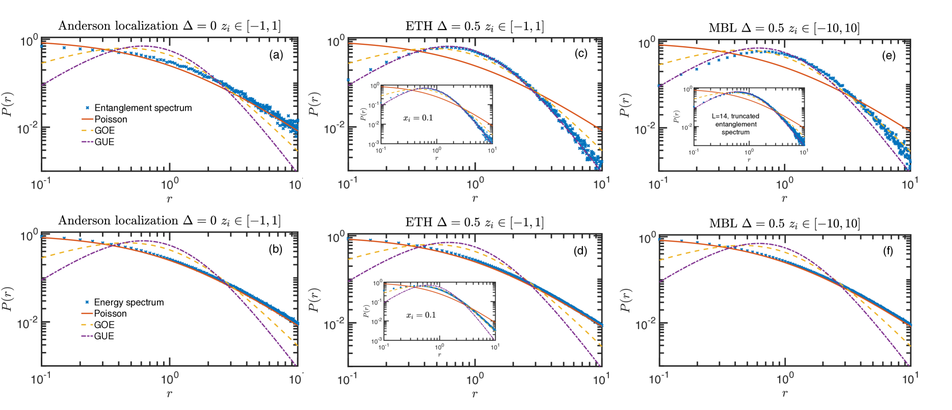
Figure 1: (Color online) Comparison between ESS and energy level spacing statistics after a quantum quench at $t_{0}=1000$ starting from a random product state in systems that are Anderson localized (a-b), nonintegrable and featuring ETH (c-d), featuring MBL (e-f). ESS follows three different distributions, namely Poisson (a), WD (c), and a non-universal one (e), thus perfectly classifying the three different dynamical phases. On the other hand, the distribution of the energy level spacings is always Poisson in all three cases. It becomes WD in the nonintegrable, ETH case shown in inset of panel (d) only if total magnetization $S_{z}$ conservation is broken by a field in the $x$ direction. In the MBL case, the ESS approaches WD upon discarding the largest eigenvalues values of the spectrum (inset of (e)). All simulations are done with $2000$ realizations of disorder and $L=12$ unless otherwise specified.

When the interaction $\Delta$ is switched on, the system can be made nonintegrable by introducing a random field $z_{i}$ xxz-affleck . Although nonintegrable, there is still a simple conserved quantity in the model, namely, the total magnetization $S_{z}$ in the $z$ direction. If the disorder is weak (we choose $h=1$) we are in case (ii): The model obeys ETH and thermalizes. At this point we are confronted with a shortcoming of the energy level statistics. For a nonintegrable system, the distribution of energy level spacings is expected to follow a WD distribution and very accurate surmises exist in this case atas13 : $P_{\rm WD}(r)=Z^{-1}(r+r^{2})^{\beta}(1+r+r^{2})^{-1-3\beta/2}$, where $Z={8}/{27}$ for the Gaussian Orthogonal Ensemble (GOE) with $\beta=1$, and $Z={4\pi}/{81\sqrt{3}}$ for the GUE with $\beta=2$. However, to find such a result one needs to diagonalize the Hamiltonian only in the subspace of fixed total magnetization kudo . If one does not know what the conserved quantities are – and this is a generic case – and diagonalizes the Hamiltonian in the full Hilbert space, one would find again Poisson statistics, see Fig. 1d. However, if one breaks the $S_{z}$ conservation by a small uniform field in the $x$ direction, one does find the WD distribution, see inset of Fig. 1d. Thus, for nonintegrable systems, one is required to know all conserved quantities in order to check the ETH through the energy level statistics. The presence of just one (local) constant of motion makes the system behave as integrable (Poisson statistics) from the viewpoint of the energy gaps if we consider the full spectrum, even though the system indeed thermalizes, while breaking all conservation laws results in WD, see Table 1.

In contrast, we find that the ESS is more robust and captures that thermalization should not be impaired by the fact that there is one conserved quantity. We find that the ESS data agrees well with a WD distribution with $\beta=2$, see Fig. 1c. Breaking the last constant of motion by introducing a small constant field $x_{i}=0.1$ in the $x$ direction results in the same distribution (see inset). Therefore, it is clear that ESS already gives us an advantage in comparison to the energy level statistics, as it can discriminate between integrable and nonintegrable models without requiring the knowledge of the local conserved quantities.

Finally, keeping fixed $\Delta=0.5$ and increasing the range of $z_{i}$ we enter in the MBL case (iii). In spite of the system being still nonintegrable, the energy eigenstates stay very localized breaking ergodicity and hence thermalization. Moreover, the eigenstates are weakly entangled (they obey an area law arealaw ; huse-mbl , which for a one-dimensional chain implies an entanglement entropy nearly independent of the system size). Thus the mechanism behind ETH breaks down and the system does not thermalize, at least within reasonable time scales, that is, nonexponential in system size. At such time scales, the system shows some features of the integrable systems, as there is an extensive number of quasilocal conserved quantities abanin1 ; abanin2 ; huse-mbl ; Louk ; chandran . This is also reflected in the distribution of the energy level spacings. We computed that distribution and show it in Fig. 1f, which reveals a Poisson statistics, just like for an integrable system (or AL, that is, integrable).

Let us now analyze the ESS for MBL. We shall find that MBL can be distinguished from both AL/integrable systems and ETH. The analysis that we present below shows that the ESS for MBL approaches asymptotically a WD distribution at rather long time scales, which we quantify below. The ESS is shown in Fig. 1e, and show the following features. At the given time scale ($t_{0}J=1000$), the ESS appears to deviate from WD statistics (as well as from Poisson statistics); the deviation is reduced if one considers a fraction of the full spectrum, retaining lowest eigenvalues values of the spectrum and discarding the largest ones (see inset). In order to quantify the approaching of the entanglement spectrum to WD (GUE) distribution upon truncation, we consider the statistical distance between two probability distributions given by the Kullback-Leibler (KL) divergence: $D_{\rm KL}(p\|q)=\sum_{i}p_{i}\log({p_{i}}/{q_{i}})$. In Fig. 2a, we show the KL divergence between $P(r)$ of MBL and the WD distribution as function of the fraction of the cutoff. As more of the largest eigenvalues values are discarded, we get closer to universal statistics. Moreover, we find that, as function of evolution time, all the $D_{KL}$ decreases as $1/\log(t)$ (see Fig. 2b), and thus the ESS of MBL asymptotically approaches a WD (GUE) distribution. (We remark that the $D_{KL}$ divergence between $P(r)$ and the WD distribution in the ETH regime goes to zero at a time scale of order $1/J$.) Indeed, in the infinite time limit, time-evolved states in the MBL regime also have to equilibrate, as the time fluctuations of typical observables go to zero, though the scaling with both time and system size are different in MBL from ETH jun .

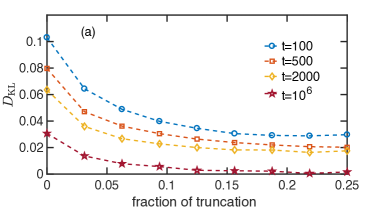
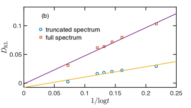
Figure 2: (Color online) (a) The KL divergence $D_{\rm KL}$ as function of the fraction of truncation of the full spectrum for different total evolution times ($L=14$ and $z_{i}\in[-8,8]$). The data are averaged over 100 realizations of disorder and 2000 realizations of the initial product state, evolved for times $t=100,500,1000$, and $10^{6}$. (b) scaling of $D_{\rm KL}$ with $1/\log(t)$ for the full spectrum and for the truncated spectrum at fraction 0.1875, consistent with the KL divergence vanishing at long times and the ESS asymtoptically reaching the WD distribution.

We interpret the slow approach to universal WD (GUE) statistics of the ESS of a state following unitary evolution with a Hamiltonian in the MBL regime as follows. At reasonable time scales, the system has approximately local conserved integrals of motion, and may look like an integrable one. However, unlike AL, the MBL Hamiltonian remains interacting even in the basis of conserved quantities. Eventually, for long time scales, information propagates along the full chain friesdorf , and the interaction between far away quasilocal conserved quantities is revealed by the slow $1/\log(t)$ approach to the universal WD distribution. The ESS detects the presence of interaction already at short time scales, because the deviations from the universal distribution are small and decreasing in time. None of these aspects can be captured by the study of the energy level spacings. We remark that this feature of the ESS is a truly dynamical one, and depends on the fact that the system is away from equilibrium. If one truncates the entanglement spectrum of a high energy eigenstate of MBL, the spectrum stays nonuniversal 2comp ; Nandkishore ; powerlaw .

Complexity of Entanglement.— The different statistics in the ESS correspond to different complexity of the entanglement generated by the time evolution. In Refs. espectrum1 ; espectrum2 , it was shown that the entanglement generated by a quantum circuit can be undone by an entanglement cooling algorithm when the ESS shows (semi-)Poisson statistics. On the other hand, if one uses a quantum circuit obtained by a universal set of gates, the ESS displays WD statistics and the simple algorithm for disentangling fails, so the ESS is complex.

How does the disentangling algorithm perform in the case of Hamiltonian evolution? We start from the final state obtained after a quantum quench for running time $t_{0}=1000$, like in the previous analysis for ESS. Notice that a similar amount of entanglement (averaged over all possible contiguous bipartitions of the system) is reached in both the MBL and the AL case (see Fig. 3), while the average entanglement is much higher for the ETH case. The disentangling (cooling) algorithm works as follows. We pick randomly a one-or two-body term from the model Eq. (1), and evolve the state for a time $\delta t=\pi/10$. Then we accept such an attempt with probability ${\rm min}\{1,{\rm exp}(-\beta\Delta\bar{S})\}$, where $\Delta\bar{S}$ is the change of the amount of von Neumann entropy averaged over all possible bipartitions of the system, and $\beta^{-1}$ is a fictitious temperature that is gradually reduced to zero.

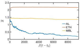
Figure 3: (Color online) Attempt of disentangling using the entanglement cooling algorithm starting from the states at $t_{0}=1000$. $\bar{S}$ is the von Neumann entropy averaged over all possible bipartitions of the system with $L=12$.

Let us look first at the cooling in the disordered XX model, which at time $t_{0}=1000$ after the quench features Poisson statistics for the ESS – what we would call a non-complex entanglement pattern. The performance of the cooling algorithm is shown in the blue curve in Fig. 3. As the data show, the state can be disentangled almost completely by this kind of entanglement cooling algorithm. It is a remarkable fact that entanglement can be undone after Hamiltonian evolution even without knowledge of the precise Hamiltonian.

What happens for ETH and MBL? Figure 3 shows that the entanglement entropy reached at $t_{0}=1000$ using both the MBL and ETH Hamiltonians cannot be undone by the cooling algorithm, even though the value of the entanglement entropy is smaller in the case of MBL. States generated from evolutions using MBL or ETH Hamiltonians cannot be disentangled, and in both cases, the ESS shows some degree of universality (both reach a WD distribution, albeit at rather different time scales). We conclude that what determines how easy or hard it is to disentangle a state is not the level of entanglement, as measured by the entanglement entropy, but instead that information is contained in the ESS, like in the case for states generated by quantum circuits.

This work is supported by DOE Grant DE-FG02-06ER46316 (Z.-C.Y. and C.C.).

References

- (1) A. Hamma, R. Ionicioiu, and P. Zanardi, Phys. Lett. A 337, 22 (2005).
- (2) A. Kitaev and J. Preskill, Phys. Rev. Lett. 96, 110404 (2006).
- (3) M. Levin and X.-G. Wen, Phys. Rev. Lett. 96, 110405 (2006).
- (4) S. M. Giampaolo and B. Hiesmayr, Phys. Rev. A 92, 012306 (2015)
- (5) S. Das, S. Shankaranarayanan, and S. Sur, Classical and Quantum Gravity Research Progress, Nova Publishers 2008; arXiv: 0806.0402.
- (6) L. Susskind, Fortsch. Phys. 64, 49 (2016).
- (7) H. Li, and F. D. M. Haldane, Phys. Rev. Lett. 101, 010504 (2008).
- (8) H. Pichler, G. Zhu, A. Seif, P. Zoller, and M. Hafezi, Phys. Rev. X 6, 041033 (2016).
- (9) C. Chamon, A. Hamma, and E. R. Mucciolo, Phys. Rev. Lett. 112, 240501 (2014).
- (10) D. Shaffer, C. Chamon, A. Hamma, and E. R. Mucciolo, J. Stat. Mech. P12007 (2014).
- (11) J. Gemmer, M. Michel, and G. Mahler, Quantum Thermodynamics – Emergence of Thermodynamic Behavior Within Composite Quantum Systems, Springer-Verlag, Heidelberg 2009.
- (12) S. Popescu, A. J. Short, and A. Winter, Nat. Phys. 2, 754–758 (2006).
- (13) S. Lloyd, Black Holes, Demons, and the Loss of Coherence. Ch. 3, Ph.D. Thesis, Rockefeller University (1988).
- (14) M. Rigol, V. Dunjko, and M. Olshanii, Nature (London) 452, 854 (2008).
- (15) P. Reimann, Phys. Rev. Lett. 99, 160404 (2007).
- (16) S. Goldstein, J. L. Leibowitz, R. Tumulka, and N. Zanghi, Phys. Rev. Lett. 96, 050403 (2006).
- (17) R. Nandkishore and D. A. Huse, Annu. Rev. Condens. Matt. Phys. 6, 15 (2015).
- (18) V. Oganesyan and D. A. Huse, Phys. Rev. B. 75, 155111 (2007).
- (19) A. Pal and D. A. Huse, Phys. Rev. B. 82, 174411 (2010).
- (20) E. Lieb, T. Schultz and D. Mattis, Ann. Phys. 16, 407–466 (1961).
- (21) E. Barouch, B. McCoy, and M. Dresden, Phys. Rev. A 2, 1075 (1970); E. Barouch and B. M. McCoy, Phys. Rev. A 3, 786 (1971).
- (22) F. Evers and A. D. Mirlin, Rev. Mod. Phys. 80, 1355 (2008).
- (23) J. M. Deutsch, Phys. Rev. A 43, 2046 (1991).
- (24) M. Srednicki, Phys. Rev. E 50, 888 (1994).
- (25) M. Žnidarič, T. Prosen, and P. Prelovšek, Phys. Rev. B. 77, 064426 (2008).
- (26) J. H. Bardarson, F. Pollmann, and J. E. Moore, Phys. Rev. Lett. 109, 017202 (2012).
- (27) M. Serbyn, Z. Papic, and D. A. Abanin, Phys. Rev. Lett. 110, 260601 (2013).
- (28) M. V. Berry and M. Tabor, Proc. Roy. Soc. A 356 375–394 (1977).
- (29) G. Montambaux, D. Poilblanc, J. Bellissard, and C. Sire, Phys. Rev. Lett. 70, 497 (1993).
- (30) P. Calabrese and J. Cardy, J. Stat. Mech. (2005) P04010.
- (31) T. Prosen, Phys. Rev. Lett. 106, 217206 (2011); R. G. Pereira, V. Pasquier, J. Sirker, and I. Affleck, J. Stat. Mech. P090307 (2014).
- (32) Y. Y. Atas, E. Bogomolny, O. Giraud, and G. Roux, Phys. Rev. Lett. 110, 084101 (2013).
- (33) K. Kudo and T. Deguchi, J. Phys. Soc. Jpn. 74, pp. 1992-2000 (2005).
- (34) J. Eisert, M. Cramer, and M. B. Plenio, Rev. Mod. Phys. 82, 277 (2010).
- (35) D. A. Huse, R. Nandkishore, and V. Oganesyan, Phys. Rev. B 90, 174202 (2014).
- (36) M. Serbyn, Z. Papic, and D. A. Abanin, Phys. Rev. Lett. 111, 127201 (2013).
- (37) I. H. Kim, A. Chandran, and D. A. Abanin, arxiv:1412.3073.
- (38) L. Rademaker and M. Ortuño, Phys. Rev. Lett. 116, 010404 (2016).
- (39) A. Chandran, I. H. Kim, G. Vidal, and D. A. Abanin, Phys. Rev. B. 91, 085425 (2015).
- (40) J. Yang, A. Hamma, arXiv:1702.00445.
- (41) M. Friesdorf, A. H. Werner, M. Goihl, J. Eisert, and W. Brown, New J. Phys. 17, 113054 (2015).
- (42) Z.-C. Yang, C. Chamon, A. Hamma, and E. R. Mucciolo, Phys. Rev. Lett. 115, 267206 (2015).
- (43) S. D. Geraedts, R. Nandkishore, and N. Regnault, Phys. Rev. B 93, 174202 (2016).
- (44) M. Serbyn, A. A. Michailidis, D. A. Abanin, and Z. Papic, Phys. Rev. Lett. 117, 160601 (2016).