Ground state degeneracy of non-Abelian topological phases
from coupled wires

Abstract

We construct a family of two-dimensional non-Abelian topological phases from coupled wires using a non-Abelian bosonization approach. We then demonstrate how to determine the nature of the non-Abelian topological order (in particular, the anyonic excitations and the topological degeneracy on the torus) realized in the resulting gapped phases of matter. This paper focuses on the detailed case study of a coupled-wire realization of the bosonic $su(2)^{\,}_{2}$ Moore-Read state, but the approach we outline here can be extended to general bosonic $su(2)^{\,}_{k}$ topological phases described by non-Abelian Chern-Simons theories. We also discuss possible generalizations of this approach to the construction of three-dimensional non-Abelian topological phases.

I Introduction

I.1 Motivation

In recent decades, topological order has emerged as a novel paradigm for describing states of matter. Motivated by the study of the fractional quantum Hall effect and chiral spin liquids, theoretical investigations uncovered a rich landscape of topologically ordered phases in two spatial dimensions. The unifying features common to all phases in this landscape are 1) the degeneracy of the ground state when the system is defined on a manifold with nonzero genus Wen (1989), and 2) the (intimately related) existence of fractionalized excitations in the gapped bulk Oshikawa and Senthil (2006). The theoretical understanding of these topologically ordered phases has been placed on a firm mathematical footing rooted in the apparatus of modular tensor categories Friedan and Shenker (1987); Fröhlich (1988); Moore and Seiberg (1989a); Fröhlich and Gabbiani (1990); Etingof et al. (2015). While numerous problems remain open to investigation, such as the inclusion of symmetries Bar (a); Teo et al. (2015); Bar (b); Tho and the description of topological phases starting from interacting electrons Gu and Wen (2014); Che (a); Kapustin et al. (2015); Gaiotto and Kapustin (2016); Ware et al. (2016); Tarantino and Fidkowski (2016); Wil , this mathematical framework provides an indispensable point of reference in the ongoing effort to understand strongly interacting topological states of matter in two spatial dimensions (2D).

Despite this progress, the construction of tractable microscopic models for topological states of matter starting from local spin or electronic degrees of freedom remains challenging. Especially challenging are chiral (i.e., time-reversal-breaking) topological phases, which cannot be represented by exactly solvable lattice models whose Hamiltonians consist of local commuting projectors Kap (in contrast to, e.g., Kitaev’s toric code and quantum double models Kitaev (2003)). There is, however, an approach that allows for the development of tractable models even in the case of chiral phases: the coupled-wire construction. In this approach, a 2D state of matter is constructed by coupling together many one-dimensional (1D) sub-systems with appropriate many-body interactions. These 1D subsystems are typically described by gapless (1+1)-dimensional effective field theories whose underlying microscopic constituents are electrons, bosons, or spins. The couplings between these subsystems can lead to fractionalization and other exotic phenomena. The utility of this approach lies in the fact that numerous analytical techniques exist for quantum field theories in (1+1)-dimensional spacetime, enabling the description of a wide variety of strongly interacting states of matter in a controlled manner. Coupled-wire constructions have been used to build a variety of strongly correlated phases in 2D, including non-Fermi liquids Emery et al. (2000); Mukhopadhyay et al. (2001); Vishwanath and Carpentier (2001) as well as Abelian and non-Abelian fractional quantum Hall states and spin liquids Poilblanc et al. (1987); Yakovenko (1991); Lee (1994); Sondhi and Yang (2001); Kane et al. (2002); Teo and Kane (2014); Mong et al. (2014); Neupert et al. (2014); Meng et al. (2015); Gorohovsky et al. (2015); Huang et al. (2016, 2017); Chen et al. (2017).

The subject of this paper is the construction and characterization of non-Abelian topological phases within the coupled-wire approach. Previous studies of coupled-wire constructions of non-Abelian topological phases have inferred the non-Abelian nature of the topological order from the structure of the edge states (e.g., their chiral central charge) when the system is studied in a cylindrical geometry (see, e.g., Refs. Teo and Kane, 2014; Meng et al., 2015; Huang et al., 2016; Chen et al., 2017). However, knowledge of the edge theory alone is insufficient to fully determine the nature of the topological order in the bulk. For example, a chiral $su(2)^{\,}_{2}$ topological phase has edge states with central charge $3/2$ that can be described by three independent chiral Majorana modes, but so does a stack of three decoupled copies of a noninteracting $p_{x}+\mathrm{i}p_{y}$ superconductor. The former topological phase has a threefold topological ground state degeneracy on the torus, while the latter does not. Thus, in order to verify the assumed correspondence between the gapless edge theory the bulk topological order in these models, it is necessary to study independently the bulk topological order itself.

In this work we construct a family of $su(2)^{\,}_{k}$ topological phases using a coupled-wire approach based on non-Abelian bosonization Witten (1984); Huang et al. (2016). This family of topological phases is putatively described at low energies by the family of $SU(2)$ Chern-Simons theories at level $k$ Witten (1989); Cabra et al. (2000). We aim to make this connection more concrete by demonstrating how to calculate the topological degeneracy on the torus of the coupled-wire construction so that it can be compared with the value $k+1$ expected from the Chern-Simons theory. Focusing on the $su(2)^{\,}_{2}$ case (which in quantum Hall terminology is known as the bosonic Moore-Read state), we show in detail how to do this within the coupled-wire setup and verify that the ground state of this model on the torus is indeed threefold degenerate. Our discussion and calculations deal at length with subtleties encountered elsewhere Oshikawa et al. (2007) in the study of non-Abelian topological phases, but has the benefit that the coupled-wire construction allows one to use explicit expressions for the operators that are used to compute the degeneracy. For a more detailed summary of our results, see Sec. I.2.

Although we study 2D topological phases in this work, another motivation for the present study is the possibility of using coupled-wire constructions to study topological phases in three dimensions (3D). The theoretical proposal Fu et al. (2007); Moore and Balents (2007) and experimental discovery Hsi ; Che (b); Hsieh et al. (2009a, b) of three-dimensional topological insulators (TIs) protected by time-reversal symmetry (TRS) underscores the natural question of what types of topological phases are possible in 3D, and whether these phases can be classified in a manner analogous to what has been achieved for 2D topological phases. Numerous examples of topologically ordered phases in three spatial dimensions have been studied theoretically. One example of such phases are so-called fractional TIs (FTIs), which are defined as gapped 3D phases with TRS whose bulk axion electromagnetic response is characterized by axion angles $\theta$ that are rational multiples of $\pi$. Consistency with TRS then demands the presence of topological order in the bulk Maciejko et al. (2010); Swingle et al. (2011). Other more elementary examples include discrete gauge theories and their twisted counterparts Dijkgraaf and Witten (1990); Wang and Wen (2015); Wan et al. (2015); Els . There also exists a procedure, the Crane-Yetter/Walker-Wang construction Crane and Yetter (1993); Walker and Wang (2012); Wang and Chen (2017); Williamson and Wang (2017), that can be used to build certain 3D topological phases. Despite this progress, the question of what kinds of strongly interacting topological phases can exist in 3D is far from settled. This is especially true of non-Abelian topological orders.

The coupled-wire approach has recently been generalized to 3D, yielding a variety of phases including Weyl semimetals Vazifeh (2013); Meng (2015), fractional topological insulators Sagi and Oreg (2015), and strongly-correlated phases described by emergent Abelian gauge theories Iadecola et al. (2016); Fuj . The goal of extending this approach to construct and characterize new non-Abelian phases in 3D is thus a natural one. The results of this paper can be used as a starting point for these investigations. In Sec. IV we provide an overview of some challenges to overcome in the extension of the non-Abelian coupled-wire approach to 3D. Given the paucity of tractable microscopic spin- and/or electron-based models for non-Abelian topological phases in 3D, we believe that the coupled-wire approach will be a valuable tool to search for and characterize candidates for new 3D topological phases of matter.

I.2 Outline and summary of results

We now provide an overview of the organization of the paper and summarize the results.

In Sec. II, we review how to bosonize a multi-flavor fermionic wire in terms of the currents associated with the non-Abelian internal symmetry group of the wire Witten (1984). This bosonization scheme has been used to address a wide variety of physical problems in 1D, including the multichannel Kondo effect Affleck (1990); Affleck and Ludwig (1991a, b) and marginally-perturbed conformal field theories (CFTs) Tsvelik (2014). In Ref. Huang et al., 2016 it was also used as a starting point for the construction of a series of non-Abelian topological phases in 2D. In Sec. II.2, we show how to add intrawire interactions to drive the fermionic wire to a strong-coupling fixed point described by an $su(2)^{\,}_{k}$ CFT. This treatment is crucial for what follows, as these CFTs are used as building blocks for the coupled-wire constructions of the subsequent sections; the non-Abelian topologically ordered phases that we construct later in the paper inherit their non-Abelian character from the $su(2)^{\,}_{k}$ CFTs.

In Sec. III, we describe how to construct non-Abelian topological phases of matter in 2D starting from a one-dimensional array of decoupled $su(2)^{\,}_{k}$ CFTs and using current-current interactions to couple channels in neighboring wires that have opposite chirality. These couplings can be viewed as arising from continuum limits of microscopic interactions between the spin sectors of neighboring wires (see, e.g., Refs. Huang et al., 2017 and Chen et al., 2017), and they are marginally relevant under the renormalization group (RG). The flow to a strong-coupling fixed point is associated to the opening of a gap in the bulk of the array of coupled wires, while leaving chiral $su(2)^{\,}_{k}$ modes on the boundaries when the model is defined on a cylinder Huang et al. (2016).

Once we have shown how to gap the bulk of the array, in Sec. III.3 we focus on the specific example of $su(2)^{\,}_{2}$ (which is related to the Moore-Read state for bosons at filling factor $\nu=1$), and show how to characterize the bulk topological order within the coupled-wire construction. The procedure for doing so hinges on using the primary operators of the unperturbed CFTs in each wire to construct nonlocal “string operators” that commute with the interaction term and satisfy a nontrivial algebra among themselves. These string operators can then be used to determine the topological ground-state degeneracy of the coupled-wire theory on the torus. More specifically, these string operators can be used to construct a representation of the ground-state manifold of the coupled-wire theory at strong coupling.

In particular, in Sec. III.3.3 we show that the algebra of these string operators suggests the algebra of Wilson loops in a $\mathbb{Z}^{\,}_{2}$ gauge theory. Namely, there are four nonlocal string operators that break into two sets of anticommuting operators. Naive intuition derived from Abelian gauge theory then suggests that the ground-state degeneracy on the torus should be fourfold. However, one finds that one of these four putative ground states cannot reside in the ground-state manifold. The reason for this has deep connections to the non-Abelian algebra of primary operators in the CFT Moore and Seiberg (1989a), and has come up before in less microscopic studies of related topological phases Oshikawa et al. (2007). In this way, we conclude that the topological degeneracy of the $su(2)^{\,}_{2}$ topological phase in 2D is three, rather than four. This exclusion of states from the ground-state manifold based on non-Abelian operator algebras is at the heart of what distinguishes non-Abelian topological phases from Abelian ones and serves as a useful operational criterion indicating when a topological phase constructed from coupled wires is non-Abelian. We expect that the techniques of Sec. III.3.3 can be extended to the other $su(2)^{\,}_{k}$ phases defined in in Sec. III.1 and used to show that these phases possess a topological degeneracy on the torus of $k+1$, in agreement with the value obtained within non-Abelian Chern Simons theory Witten (1989); Cabra et al. (2000).

In Sec. IV we provide an overview of prospects for generalizing the construction presented in this paper to 3D. We identify challenges that make such a generalization a delicate matter, and we propose several possible ways of overcoming these challenges. We believe that these observations will help to define a path forward for the use of coupled-wire constructions in the construction of new non-Abelian phases of matter in 3D.

II Non-Abelian bosonization of a single wire

II.1 Free-fermion wire

Consider a one-dimensional wire containing $N^{\,}_{\mathrm{c}}$ “colors” (orbitals) of spinful fermions. Its action $S^{\,}_{0,\mathrm{wire}}$ is the integral over time $t$ and the coordinate $z$ along the wire of the Lagrangian density

$$\begin{split}\mathcal{L}^{\,}_{0,\mathrm{wire}}\,\raisebox{0.85pt}{.}\raisebox{2.85pt}{.}\!\!=\,2\sum_{\sigma=\uparrow,\downarrow}\sum^{N^{\,}_{\mathrm{c}}}_{\alpha=1}\Big{(}&\chi^{*}_{\mathrm{L},\sigma,\alpha}\,\mathrm{i}\partial^{\,}_{\mathrm{L}}\chi^{\,}_{\mathrm{L},\sigma,\alpha}\\ &+\chi^{*}_{\mathrm{R},\sigma,\alpha}\,\mathrm{i}\partial^{\,}_{\mathrm{R}}\chi^{\,}_{\mathrm{R},\sigma,\alpha}\Big{)}.\end{split}$$ (1)

The derivatives $\partial^{\,}_{\mathrm{M}}\equiv\partial^{\,}_{z^{\,}_{\mathrm{M}}}$ ($\mathrm{M}=\mathrm{L},\mathrm{R}$) are taken with respect to the chiral (light-cone) coordinates

$$z^{\,}_{\mathrm{L}}\equiv t+z,\qquad z^{\,}_{\mathrm{R}}\equiv t-z.$$ (2)

We assume periodic boundary conditions along the wire, i.e., in the $z$-direction. The four Grassmann-valued fields $\chi^{*}_{\mathrm{L},\sigma,\alpha}$, $\chi^{\,}_{\mathrm{L},\sigma,\alpha}$, $\chi^{*}_{\mathrm{R},\sigma,\alpha}$, $\chi^{\,}_{\mathrm{R},\sigma,\alpha}$ are independent of each other.

Such a wire has the internal symmetry $U(2N^{\,}_{\mathrm{c}})^{\,}_{\mathrm{L}}\times U(2N^{\,}_{\mathrm{c}})^{\,}_{\mathrm{R}}$. The central idea of the coupled-wire constructions presented in this paper is to decompose the Lie algebra associated with this symmetry using the following identity (or “conformal embedding”) Di Francesco et al. (1997),

$$u(2N^{\,}_{\mathrm{c}})^{\,}_{1}=u(1)\oplus su(2)^{\,}_{N^{\,}_{\mathrm{c}}}\oplus su(N^{\,}_{\mathrm{c}})^{\,}_{2},$$ (3)

where we have employed the notation $g^{\,}_{k}$ for the affine Lie algebra at level $k$ associated with the connected, compact, and simple Lie group $G$. (For a review of affine Lie algebras, see, e.g., Ref. Di Francesco et al., 1997.) Equation (3) tells us that the theory (1) has three conserved currents $j^{\,}_{\mathrm{R}}$, $J^{a}_{\mathrm{R}}$, and $\mathsf{J}^{\mathsf{a}}_{\mathrm{R}}$ corresponding to the affine Lie algebras $u(1)$, $su(2)^{\,}_{N^{\,}_{\mathrm{c}}}$, and $su(N^{\,}_{\mathrm{c}})^{\,}_{2}$, respectively. (Note that, of course, there are analogous conserved currents $j^{\,}_{\mathrm{L}},J^{a}_{\mathrm{L}},$ and $\mathsf{J}^{\mathsf{a}}_{\mathrm{L}}$ for the left-handed sector.) We use indices $a=1,2,3$ to label the generators of $SU(2)$ and $\mathsf{a}=1,\cdots,N^{2}_{\mathrm{c}}-1$ to label the generators of $SU(N^{\,}_{\mathrm{c}})$. In terms of the complex fermions, these currents are given by

$$j^{\,}_{\mathrm{M}}\,\raisebox{0.85pt}{.}\raisebox{2.85pt}{.}\!\!=\,\sum_{\sigma=\uparrow,\downarrow}\sum^{N^{\,}_{\mathrm{c}}}_{\alpha=1}\chi^{*}_{\mathrm{M},\sigma,\alpha}\,\chi^{\,}_{\mathrm{M},\sigma,\alpha},$$ (4a)

$$J^{a}_{\mathrm{M}}\,\raisebox{0.85pt}{.}\raisebox{2.85pt}{.}\!\!=\,\frac{1}{2}\sum_{\sigma,\sigma^{\prime}=\uparrow,\downarrow}\sum^{N^{\,}_{\mathrm{c}}}_{\alpha=1}\chi^{*}_{\mathrm{M},\sigma,\alpha}\,\sigma^{a}_{\sigma\sigma^{\prime}}\,\chi^{\,}_{\mathrm{M},\sigma^{\prime},\alpha},$$ (4b)

$$\mathsf{J}^{\mathsf{a}}_{\mathrm{M}}\,\raisebox{0.85pt}{.}\raisebox{2.85pt}{.}\!\!=\,\sum_{\sigma=\uparrow,\downarrow}\sum^{N^{\,}_{\mathrm{c}}}_{\alpha,\alpha^{\prime}=1}\chi^{*}_{\mathrm{M},\sigma,\alpha}\,T^{\mathsf{a}}_{\alpha\alpha^{\prime}}\,\chi^{\,}_{\mathrm{M},\sigma,\alpha^{\prime}},$$ (4c)

with $\mathrm{M}=\mathrm{L},\mathrm{R}$. The $U(1)$ currents $j^{\,}_{\mathrm{M}}$ with $\mathrm{M}=\mathrm{L},\mathrm{R}$ are associated with charge conservation. The $SU(2)$ currents $J^{a}_{\mathrm{M}}$ with $\mathrm{M}=\mathrm{L},\mathrm{R}$ and $a=1,2,3$ are associated with the spin-rotation symmetry. The $SU(N^{\,}_{\mathrm{c}})$ currents $\mathsf{J}^{\mathsf{a}}_{\mathrm{M}}$ with $\mathrm{M}=\mathrm{L},\mathrm{R}$ and $\mathsf{a}=1,\cdots,N^{2}_{\mathrm{c}}-1$ are associated with the color isospin-rotation symmetry. The generators $\sigma^{a}/2$ of $SU(2)$ and $T^{\mathsf{a}}$ of $SU(N^{\,}_{\mathrm{c}})$ obey the normalizations and the independent algebras

$$\mathrm{tr}\,\left(\sigma^{a}\,\sigma^{b}\right)=2\delta^{ab},\qquad[\sigma^{a},\sigma^{b}]=2\mathrm{i}\,\epsilon^{abc}\,\sigma^{c},$$ (5a)

$$\mathrm{tr}\,\left(T^{\mathsf{a}}\,T^{\mathsf{b}}\right)=\frac{1}{2}\delta^{\mathsf{ab}},\qquad[T^{\mathsf{a}},T^{\mathsf{b}}]=\mathrm{i}\,f^{\mathsf{abc}}\,T^{\mathsf{c}},$$ (5b)

where $\epsilon^{\,}_{abc}$ is the Levi-Civita symbol and $f^{\,}_{\mathsf{abc}}$ are the structure constants of $SU(N^{\,}_{\mathrm{c}})$. With these definitions, one can build the energy-momentum tensor for the free theory defined by the Lagrangian density (1) using the Sugawara construction Sugawara (1968); Affleck (1990); Affleck and Ludwig (1991a, b) for the energy-momentum tensor in the M-moving sector,

$$T^{\,}_{\mathrm{M}}[u(2N^{\,}_{\mathrm{c}})^{\,}_{1}]=T^{\,}_{\mathrm{M}}[u(1)]+T^{\,}_{\mathrm{M}}[su(2)^{\,}_{N^{\,}_{\mathrm{c}}}]+T^{\,}_{\mathrm{M}}[su(N^{\,}_{\mathrm{c}})^{\,}_{2}].$$ (6a)

Here,

$$T^{\,}_{\mathrm{M}}[u(2N^{\,}_{\mathrm{c}})^{\,}_{1}]\,\raisebox{0.85pt}{.}\raisebox{2.85pt}{.}\!\!=\,\frac{1}{\pi}\sum_{\sigma=\uparrow,\downarrow}\sum^{N^{\,}_{\mathrm{c}}}_{\alpha=1}\chi^{*}_{\mathrm{M},\sigma,\alpha}\,\mathrm{i}\partial^{\,}_{\mathrm{M}}\chi^{\,}_{\mathrm{M},\sigma,\alpha},$$ (6b)

$$T^{\,}_{\mathrm{M}}[u(1)]\,\raisebox{0.85pt}{.}\raisebox{2.85pt}{.}\!\!=\,\frac{1}{4N^{\,}_{\mathrm{c}}}\,j^{\,}_{\mathrm{M}}\,j^{\,}_{\mathrm{M}},$$ (6c)

$$T^{\,}_{\mathrm{M}}[su(2)^{\,}_{N^{\,}_{\mathrm{c}}}]\,\raisebox{0.85pt}{.}\raisebox{2.85pt}{.}\!\!=\,\frac{1}{N^{\,}_{\mathrm{c}}+2}\sum^{3}_{a=1}J^{a}_{\mathrm{M}}\,J^{a}_{\mathrm{M}},$$ (6d)

$$T^{\,}_{\mathrm{M}}[su(N^{\,}_{\mathrm{c}})^{\,}_{2}]\,\raisebox{0.85pt}{.}\raisebox{2.85pt}{.}\!\!=\,\frac{1}{2+N^{\,}_{\mathrm{c}}}\sum^{N^{2}_{\mathrm{c}}-1}_{\mathsf{a}=1}\mathsf{J}^{\mathsf{a}}_{\mathrm{M}}\,\mathsf{J}^{\mathsf{a}}_{\mathrm{M}}.$$ (6e)

With these definitions, it follows that the Hamiltonian density associated with the free Lagrangian density (1) is given by

$$\mathcal{H}^{\,}_{0,\mathrm{wire}}\!\!\,\raisebox{0.85pt}{.}\raisebox{2.85pt}{.}\!\!=\,\!\!2\pi\!\!\!\!\!\sum_{\mathrm{M}=\mathrm{L},\mathrm{R}}\!\!\!\!\left(T^{\,}_{\mathrm{M}}[u(1)]\!+\!T^{\,}_{\mathrm{M}}[su(2)^{\,}_{N^{\,}_{\mathrm{c}}}]\!+\!T^{\,}_{\mathrm{M}}[su(N^{\,}_{\mathrm{c}})^{\,}_{2}]\right)\!.$$ (7)

Rewriting the free theory (1) in terms of the currents (4) amounts to performing a non-Abelian bosonization of the free theory. This rewriting highlights the fact that a theory of multiple flavors of free fermions can be broken up into independent charge [$u(1)$], spin [$su(2)^{\,}_{N^{\,}_{\mathrm{c}}}$], and color (orbital) [$su(N^{\,}_{\mathrm{c}})^{\,}_{2}$] sectors.

II.2 Intrawire interactions

Having rewritten the free theory (1) in terms of the non-Abelian currents (4), we now wish to isolate the $su(2)^{\,}_{N^{\,}_{\mathrm{c}}}$ spin degrees of freedom by removing the $u(1)$ charge and $su(N^{\,}_{\mathrm{c}})^{\,}_{2}$ color (orbital) degrees of freedom from the low-energy sector of the theory. We accomplish this by adding interactions that gap out the latter pair of degrees of freedom.

To gap out the charge sector, we add to the free Lagrangian density (1) the interaction term

$$\mathcal{L}^{\,}_{\mathrm{int}}[u(1)]\,\raisebox{0.85pt}{.}\raisebox{2.85pt}{.}\!\!=\,-\lambda^{\,}_{u(1)}\cos\left(\sqrt{2}\,(\phi^{\,}_{\mathrm{R}}+\phi^{\,}_{\mathrm{L}})\right).$$ (8a)

The chiral bosonic fields $$\phi^{\,}_{\mathrm{M}}$$ are defined by the Abelian bosonization identity

$$j^{\,}_{\mathrm{M}}=-\frac{1}{\sqrt{2}\,\pi}\,\partial^{\,}_{\mathrm{M}}\phi^{\,}_{\mathrm{M}}.$$ (8b)

In the fermionic language, the interaction (8a) is interpreted as an Umklapp process. It is marginally relevant in the renormalization group (RG) sense, i.e., it flows to strong coupling under RG and gaps the charge sector when $\lambda^{\,}_{u(1)}>0$.

To gap out the color (orbital) sector, we add to the free Lagrangian density (1) the interaction term

$$\mathcal{L}^{\,}_{\mathrm{int}}[su(N^{\,}_{\mathrm{c}})^{\,}_{2}]\,\raisebox{0.85pt}{.}\raisebox{2.85pt}{.}\!\!=\,-\lambda^{\,}_{su(N^{\,}_{\mathrm{c}})^{\,}_{2}}\sum^{N^{2}_{\mathrm{c}}-1}_{\mathsf{a}=1}\mathsf{J}^{\mathsf{a}}_{\mathrm{L}}\,\mathsf{J}^{\mathsf{a}}_{\mathrm{R}},$$ (9)

where the currents $\mathsf{J}^{\mathsf{a}}_{\mathrm{M}}$ are defined in Eqs. (4). This current-current interaction is also marginally relevant, flowing to strong coupling for $\lambda^{\,}_{su(N^{\,}_{\mathrm{c}})^{\,}_{2}}>0$.

At the strong-coupling fixed point dominated by the interactions (8) and (9), the effective Hamiltonian density for the low-energy sector becomes

$$\mathcal{H}^{\,}_{0,\mathrm{eff}}\,\raisebox{0.85pt}{.}\raisebox{2.85pt}{.}\!\!=\,2\pi\left(T^{\,}_{\mathrm{L}}[su(2)^{\,}_{N^{\,}_{\mathrm{c}}}]+T^{\,}_{\mathrm{R}}[su(2)^{\,}_{N^{\,}_{\mathrm{c}}}]\right).$$ (10)

This is nothing but the Hamiltonian description of the $su(2)^{\,}_{N^{\,}_{\mathrm{c}}}$ Wess-Zumino-Witten (WZW) CFT Wess and Zumino (1971); Witten (1984) with the central charge

$$c[su(2)^{\,}_{N^{\,}_{\mathrm{c}}}]=\frac{3\,N^{\,}_{\mathrm{c}}}{2+N^{\,}_{\mathrm{c}}}.$$ (11)

Thus, by adding the interactions (8) and (9) to the free theory (1), we can convert a quantum wire containing $N^{\,}_{\mathrm{c}}$ colors (orbitals) of spinful fermions into a highly nontrivial CFT. The coupled-wire constructions presented in this paper use arrays of these $su(2)^{\,}_{N^{\,}_{\mathrm{c}}}$ WZW theories as building blocks for non-Abelian topological phases.

III Non-Abelian topological order in two dimensions

In this section we construct a class of $su(2)^{\,}_{k}$ topological quantum liquids in two spatial dimensions and show, for the case of $k=2$, how to compute their topological degeneracy on the torus. This analysis yields new insights for the description of non-Abelian topological phases with coupled wires.

III.1 Definition of the class of models

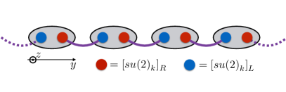
Figure 1: (Color online) Schematic of the coupled-wire construction for $su(2)^{\,}_{k}$ non-Abelian topological orders in two spatial dimensions. Grey ovals represent quantum wires, while red and blue circles represent chiral $su(2)^{\,}_{k}$ currents.

We begin with a one-dimensional array $\Lambda$ of parallel nonchiral spinful fermionic quantum wires aligned along the $z$-direction, each of which is described by the Lagrangian density (1) (see Fig. 1). The cardinality of the one-dimensional lattice $\Lambda$ is

$$|\Lambda|\equiv L^{\,}_{y}+1.$$ (12)

We set $N^{\,}_{\mathrm{c}}=k$, where $N^{\,}_{\mathrm{c}}$ is the number of “colors” (orbitals) of fermions in each wire. Each wire has an internal symmetry $U(2k)^{\,}_{\mathrm{L}}\times U(2k)^{\,}_{\mathrm{R}}$, with respect to which we carry out the bosonization procedure of Sec. II. We then gap the $u(1)$ and $su(k)^{\,}_{2}$ sectors with the intrawire interactions discussed in Sec. II.1, leaving behind an $su(2)^{\,}_{k}$ current algebra for each of the left- and right-moving chiral sectors in every wire. In the Heisenberg picture and in two-dimensional Minkowski space, we denote the chiral $su(2)^{\,}_{k}$ currents by $\widehat{J}^{a}_{\mathrm{M},y}(z^{\,}_{\mathrm{M}})$ where $\mathrm{M}=\mathrm{L},\mathrm{R}$ labels the chirality, $a=1,2,3$ labels the $SU(2)$ generators, $y$ labels the wire, and $z^{\,}_{\mathrm{M}}$ is defined in Eq. (2).

We couple nearest-neighbor wires with the $su(2)^{\,}_{k}$ interaction (see Fig. 1)

$$\widehat{\mathcal{L}}^{\,}_{\mathrm{bs}}\equiv-\widehat{\mathcal{H}}^{\,}_{\mathrm{bs}}\,\raisebox{0.85pt}{.}\raisebox{2.85pt}{.}\!\!=\,-\frac{\lambda}{2}\sum_{y=0}^{L^{\,}_{y}-\sigma^{\,}_{\mathrm{BC}}}\left(\widehat{J}^{+}_{\mathrm{L},y+1}\,\widehat{J}^{-}_{\mathrm{R},y}+\mathrm{H.c.}\right),$$ (13a)

where $$\sigma^{\,}_{\mathrm{BC}}=0,1$$ for periodic and open boundary conditions, respectively. In Eq. (13), we have introduced the linear combinations

$$\widehat{J}^{\pm}_{\mathrm{M},y}\,\raisebox{0.85pt}{.}\raisebox{2.85pt}{.}\!\!=\,\widehat{J}^{1}_{\mathrm{M},y}\pm\mathrm{i}\,\widehat{J}^{2}_{\mathrm{M},y}.$$ (13b)

When periodic boundary conditions are imposed in the $y$-direction, i.e., when $\sigma^{\,}_{\mathrm{BC}}=0$, each chiral current is paired with exactly one current of the opposite chirality in a neighboring wire, and, hence, the full array of quantum wires may become gapped in the strong-coupling limit $|\lambda|\gg 0$. Indeed, similar interactions were used in Ref. Huang et al., 2016 to construct a large class of topological phases, including the class of $su(2)^{\,}_{k}$ phases discussed here. These interactions are marginally relevant under RG, and their flow to strong coupling is associated with the opening of a bulk gap in the array of coupled wires when $\sigma^{\,}_{\mathrm{BC}}=0$. When open boundary conditions are imposed in the $y$-direction, i.e., when $\sigma^{\,}_{\mathrm{BC}}=1$, there is a left-moving $su(2)^{\,}_{k}$ current at $y=0$ and a right-moving $su(2)^{\,}_{k}$ current at $y=L^{\,}_{y}$ that are fully decoupled from the bulk. This edge structure is reminiscent of that of the $su(2)^{\,}_{k}$ non-Abelian Chern-Simons theories Witten (1989); Cabra et al. (2000) and that of the $\mathbb{Z}^{\,}_{k}$ Read-Rezayi quantum Hall states Read and Rezayi (1999).

III.2 Parafermion representation of the interwire interactions

The interaction (13) can be better understood by rewriting the $su(2)^{\,}_{k}$ currents in terms of auxiliary degrees of freedom. This rewriting must preserve the $su(2)^{\,}_{k}$ current algebra, which is encoded in the operator product expansion (OPE) Di Francesco et al. (1997)

$$\widehat{J}^{a}_{\mathrm{L},y}(v)\,\widehat{J}^{\tilde{a}}_{\mathrm{L},\tilde{y}}(w)\sim\delta^{\,}_{y,\tilde{y}}\,\left(\frac{(k/2)\,\delta^{a\tilde{a}}}{v^{2}-w^{2}}+\frac{\mathrm{i}\,\epsilon^{a\tilde{a}b}\,\widehat{J}^{b}_{\mathrm{L},y}(w)}{v-w}\right),$$ (14)

for the holomorphic sector $\mathrm{M}=\mathrm{L}$, and similarly for the antiholomorphic sector $\mathrm{M}=\mathrm{R}$. (Here, we employ complex coordinates $v\equiv t+\mathrm{i}\,z$, obtained from the chiral coordinate $z^{\,}_{\mathrm{L}}$ defined in Eq. (2) by the analytic continuation $z\to\mathrm{i}\,z$, and $\bar{v}\equiv t-\mathrm{i}\,z$, obtained from the chiral coordinate $z^{\,}_{\mathrm{R}}$ also defined in Eq. (2) by the same analytic continuation.) The group indices $a,\tilde{a}=1,2,3$, and summation over the repeated index $b=1,2,3$ is implied. The symbol $``\sim"$ denotes equality up to nonsingular terms in the limit $v\to w$.

As shown by Zamolodchikov and Fateev Zamolodchikov and Fateev (1985) (see Appendix A), the current algebra (14) can be represented in terms of $\mathbb{Z}^{\,}_{k}$ parafermion and chiral boson operators by [see Eq. (5.5) from Ref. Zamolodchikov and Fateev, 1985]

$$\widehat{J}^{+}_{\mathrm{M},y}\,=\!\!\raisebox{0.85pt}{.}\raisebox{2.85pt}{.}\,\sqrt{k}\ \widehat{\Psi}^{\,}_{\mathrm{M},y}\,\bm{:}e^{+\mathrm{i}\sqrt{1/k}\,\widehat{\phi}^{\,}_{\mathrm{M},y}}\bm{:},$$ (15a)

$$\widehat{J}^{-}_{\mathrm{M},y}\,=\!\!\raisebox{0.85pt}{.}\raisebox{2.85pt}{.}\,\sqrt{k}\ \bm{:}e^{-\mathrm{i}\sqrt{1/k}\,\widehat{\phi}^{\,}_{\mathrm{M},y}}\bm{:}\,\widehat{\Psi}^{{\dagger}}_{\mathrm{M},y},$$ (15b)

$$\widehat{J}^{3}_{\mathrm{M},y}\,=\!\!\raisebox{0.85pt}{.}\raisebox{2.85pt}{.}\,\mathrm{i}\,\frac{\sqrt{k}}{2}\,\partial^{\,}_{\mathrm{M}}\widehat{\phi}^{\,}_{\mathrm{M},y},$$ (15c)

where $\bm{:}\cdot\bm{:}$ denotes normal ordering with respect to the many-body ground state of $\widehat{H}^{\,}_{0,\mathrm{eff}}$ within each wire. Here, the $\mathbb{Z}^{\,}_{k}$ parafermions $\widehat{\Psi}^{\,}_{\mathrm{M},y}$ satisfy the equal-time algebra

$$\begin{split}&\widehat{\Psi}^{\,}_{\mathrm{M},y}(t,z)\,\widehat{\Psi}^{\,}_{\mathrm{M}^{\prime},y^{\prime}}(t,z^{\prime})=\widehat{\Psi}^{\,}_{\mathrm{M}^{\prime},y^{\prime}}(t,z^{\prime})\,\widehat{\Psi}^{\,}_{\mathrm{M},y}(t,z)\,e^{-\mathrm{i}\,\frac{2\pi}{k}\,\delta^{\,}_{y,y^{\prime}}\left[(-1)^{\mathrm{M}}\,\delta^{\,}_{\mathrm{M},\mathrm{M}^{\prime}}\,\mathrm{sgn}(z-z^{\prime})+\epsilon^{\,}_{\mathrm{M},\mathrm{M}^{\prime}}\right]+\mathrm{i}\,\frac{2\pi}{k}\,\mathrm{sgn}(y-y^{\prime})},\end{split}$$ (16a)

$$\begin{split}&\widehat{\Psi}^{{\dagger}}_{\mathrm{M},y}(t,z)\,\widehat{\Psi}^{{\dagger}}_{\mathrm{M}^{\prime},y^{\prime}}(t,z^{\prime})=\widehat{\Psi}^{{\dagger}}_{\mathrm{M}^{\prime},y^{\prime}}(t,z^{\prime})\,\widehat{\Psi}^{{\dagger}}_{\mathrm{M},y}(t,z)\,e^{-\mathrm{i}\,\frac{2\pi}{k}\,\delta^{\,}_{y,y^{\prime}}\left[(-1)^{\mathrm{M}}\,\delta^{\,}_{\mathrm{M},\mathrm{M}^{\prime}}\,\mathrm{sgn}(z-z^{\prime})+\epsilon^{\,}_{\mathrm{M},\mathrm{M}^{\prime}}\right]+\mathrm{i}\,\frac{2\pi}{k}\,\mathrm{sgn}(y-y^{\prime})},\end{split}$$ (16b)

$$\begin{split}&\widehat{\Psi}^{\,}_{\mathrm{M},y}(t,z)\,\widehat{\Psi}^{{\dagger}}_{\mathrm{M}^{\prime},y^{\prime}}(t,z^{\prime})=\widehat{\Psi}^{{\dagger}}_{\mathrm{M}^{\prime},y^{\prime}}(t,z^{\prime})\,\widehat{\Psi}^{\,}_{\mathrm{M},y}(t,z)\,e^{+\mathrm{i}\,\frac{2\pi}{k}\,\delta^{\,}_{y,y^{\prime}}\left[(-1)^{\mathrm{M}}\,\delta^{\,}_{\mathrm{M},\mathrm{M}^{\prime}}\,\mathrm{sgn}(z-z^{\prime})+\epsilon^{\,}_{\mathrm{M},\mathrm{M}^{\prime}}\right]-\mathrm{i}\,\frac{2\pi}{k}\,\mathrm{sgn}(y-y^{\prime})}.\end{split}$$ (16c)

The sign function above is defined such that $$\mathrm{sgn}(0)=0 \mathrm{M}=\mathrm{L},\mathrm{R} \epsilon^{\,}_{\mathrm{M},\mathrm{M}^{\prime}} \epsilon^{\,}_{\mathrm{L},\mathrm{R}}=-\epsilon^{\,}_{\mathrm{R},\mathrm{L}}=1 (-1)^{\mathrm{R}}=-(-1)^{\mathrm{L}}\equiv 1 su(2)^{\,}_{k}$$. The left- and right-moving labels are defined with the convention that is the antisymmetric Levi-Civita symbol obeying . Moreover, . The algebra of the currents holds so long as the equal-time algebra

$$\begin{split}&\left[\widehat{\phi}^{\,}_{\mathrm{M},y}(t,z),\widehat{\phi}^{\,}_{\mathrm{M}^{\prime},y^{\prime}}(t,z^{\prime})\right]=-\mathrm{i}\,2\pi\left[(-1)^{\mathrm{M}}\,\delta^{\,}_{y,y^{\prime}}\,\delta^{\,}_{\mathrm{M},\mathrm{M}^{\prime}}\,\mathrm{sgn}(z-z^{\prime})+\delta^{\,}_{y,y^{\prime}}\,\epsilon^{\,}_{\mathrm{M},\mathrm{M}^{\prime}}-\mathrm{sgn}(y-y^{\prime})\right],\end{split}$$ (16d)

is imposed in the chiral bosonic sector. In particular, one verifies that currents defined in different wires commute with one another at equal times when the definitions (15) are imposed. Furthermore, one can show that all equal-time commutators between $su(2)^{\,}_{k}$ currents differing by their $\mathrm{L}$ and $\mathrm{R}$ labels also vanish. Finally, the chiral parafermions commute with the chiral bosons at equal times.

The representation (15) of the $su(2)^{\,}_{k}$ current algebra provides a convenient interpretation of the interactions (13) in terms of fractionalized degrees of freedom, as we discuss below. However, there are several caveats to keep in mind. Chief among these is the fact that the factorization (15)–(15) of the $su(2)^{\,}_{k}$ currents re-expresses a set of local operators (the currents) in terms of products of auxiliary degrees of freedom (the parafermions and the chiral bosons). While the $su(2)^{\,}_{k}$ currents admit a local expression [Eq. (4b)] in terms of the original degrees of freedom used to define the theory (the electrons) these auxiliary degrees of freedom do not. This fact will be important when we construct the nonlocal string operators that allow us to calculate the topological degeneracy in Sec. III.3. Furthermore, we note that this parafermion representation is not unique in two ways. First, as it factorizes a local (observable) operator into the product of two operators, there is an ambiguity with the choice of the phase assigned to each operator-valued factor. (This is an explicit manifestation of the nonlocality of the auxiliary degrees of freedom.) The choice for this phase cannot have observable consequences. Second, the dependence on the labels $y\neq y^{\prime}$ of the equal-time algebra is not unique since many distinct choices accommodate the fact that any two currents belonging to two distinct wires $y$ and $y^{\prime}$ must always commute. Hence, the dependence on the labels $y\neq y^{\prime}$ of the parafermion equal-time algebra cannot have observable consequences. We demonstrate that this is true for the case of $su(2)^{\,}_{2}$ in Appendix D.

We work with the normalization convention for which the operator $\exp(\mathrm{i}\,a\,\widehat{\phi}^{\,}_{\mathrm{M}})$, for $a$ any real-valued number, has the conformal weights $(a^{2},0)$ if $\mathrm{M}=\mathrm{L}$ or $(0,a^{2})$ if $\mathrm{M}=\mathrm{R}$. With this convention, the chiral vertex operator $\exp(\mathrm{i}\,\sqrt{1/k}\,\widehat{\phi}^{\,}_{\mathrm{M}})$, which annihilates a chiral Abelian quasiparticle, has the conformal weights $(1/k,0)$ if $\mathrm{M}=\mathrm{L}$ or $(0,1/k)$ if $\mathrm{M}=\mathrm{R}$. In turn, the chiral parafermion operator $\widehat{\Psi}^{\,}_{\mathrm{M}}$ must have the conformal weights $(1-1/k,0)$ if $\mathrm{M}=\mathrm{L}$ or $(0,1-1/k)$ if $\mathrm{M}=\mathrm{R}$, as the current operators have the conformal weights $(1,0)$ if $\mathrm{M}=\mathrm{L}$ or $(0,1)$ if $\mathrm{M}=\mathrm{R}$. The expressions (15) for the currents are equivalent to the identity Di Francesco et al. (1997)

$$su(2)^{\,}_{k}\simeq u(1)^{\,}_{k}\oplus\mathbb{Z}^{\,}_{k},$$ (17a)

where

$$\mathbb{Z}^{\,}_{k}\equiv\frac{su(2)^{\,}_{k}}{u(1)^{\,}_{k}},$$ (17b)

which states that an $SU(2)$ WZW theory at level $k$ can be interpreted as a direct product of a chiral boson and a $\mathbb{Z}^{\,}_{k}$ parafermion CFT.

With these definitions, the interactions (13) take the form

$$\widehat{\mathcal{L}}^{\,}_{\mathrm{bs}}\equiv-\widehat{\mathcal{H}}^{\,}_{\mathrm{bs}} =\,-\lambda\,\frac{k}{2}\,\sum^{L^{\,}_{y}}_{y=0}\,\left(\widehat{\Psi}^{\,}_{\mathrm{L},y}\,\bm{:}e^{+\mathrm{i}\sqrt{\frac{1}{k}}\,\widehat{\phi}^{\,}_{\mathrm{L},y}}\bm{:}\,\bm{:}e^{-\mathrm{i}\sqrt{\frac{1}{k}}\,\widehat{\phi}^{\,}_{\mathrm{R},y+1}}\bm{:}\,\widehat{\Psi}^{{\dagger}}_{\mathrm{R},y+1}\,+\mathrm{H.c.}\right),$$ (18)

(We employ periodic boundary conditions for the remainder of this section.) Written this way, the current-current interactions (13) can be reinterpreted as correlated hoppings of (nonlocal) fractionalized degrees of freedom between wires. Indeed, viewing $\widehat{\Psi}^{{\dagger}}_{\mathrm{M},y}$ as the creation operator for a parafermion with chirality $\mathrm{M}$ in wire $y$, and viewing the vertex operator $\bm{:}e^{-\mathrm{i}\sqrt{\frac{1}{k}}\,\widehat{\phi}^{\,}_{\mathrm{M},y}}\bm{:}$ as the creation operator for an Abelian quasiparticle, we can interpret Eq. (18) as allowing parafermions to hop between wires so long as an Abelian quasiparticle hops at the same time. Since the composite of these two fractionalized excitations is a boson, per Eqs. (15), this correlated hopping process forbids isolated fractionalized degrees of freedom from hopping between wires.

When periodic boundary conditions are imposed, the interaction (18) gaps out the array of wires if the current-current coupling on each bond in the lattice $\Lambda$ acquires a finite vacuum expectation value. Such a scenario is possible in the limit $\lambda\to\infty$. We will see an explicit example of this gapping mechanism in the next section.

III.3 Case study: $su(2)^{\,}_{2}$

In this section, we work through the example of $k=2$ in detail. First, we will examine more closely how the interaction (18) leads to a gapped state of matter. Next, we will characterize the topological order in this gapped state of matter by imposing periodic boundary conditions in the $y$- and $z$-directions and constructing nonlocal string operators that commute with the interaction $\widehat{\mathcal{H}}^{\,}_{\mathrm{bs}}$ defined by Eq. (13). These string operators will label the topologically degenerate ground states in the limit $\lambda\to\infty$.

The Lagrangian density in this case is (omitting the normal ordering of the vertex operators)

$$\widehat{\mathcal{L}}^{\,}_{\mathrm{bs}}\equiv-\widehat{\mathcal{H}}^{\,}_{\mathrm{bs}} \,\raisebox{0.85pt}{.}\raisebox{2.85pt}{.}\!\!=\,-\lambda\sum_{y=0}^{L^{\,}_{y}}\left(e^{+\mathrm{i}\sqrt{1/2}\,\left(\widehat{\phi}^{\,}_{\mathrm{L},y}-\widehat{\phi}^{\,}_{\mathrm{R},y+1}\right)}\,\widehat{\psi}^{\,}_{\mathrm{L},y}\,\widehat{\psi}^{\,}_{\mathrm{R},y+1}+\mathrm{H.c.}\right)$$ (19a)

$$=-2\lambda\sum_{y=0}^{L^{\,}_{y}}\left(\mathrm{i}\,\widehat{\psi}^{\,}_{\mathrm{L},y}\,\widehat{\psi}^{\,}_{\mathrm{R},y+1}\right)\sin\left(\sqrt{\frac{1}{2}}\left(\widehat{\phi}^{\,}_{\mathrm{L},y}-\widehat{\phi}^{\,}_{\mathrm{R},y+1}\right)\right),$$ (19b)

which should be compared with Eq. (18). The chiral operators

$$\widehat{\psi}^{\,}_{\mathrm{M},y}(t,z)\equiv\widehat{\Psi}^{\,}_{\mathrm{M},y}(t,z)\equiv\widehat{\Psi}^{{\dagger}}_{\mathrm{M},y}(t,z)$$ (20a)

with $$\mathrm{M}=\mathrm{L},\mathrm{R} \mathbb{Z}^{\,}_{2} k=2$$ are Majorana operators (i.e., parafermions). Their equal-time exchange algebra is given by Eq. (16a) with . We also impose the normalization

$$\lim_{z^{\prime}\to z}\widehat{\psi}^{\,}_{\mathrm{M},y}(t,z)\,\widehat{\psi}^{\,}_{\mathrm{M},y}(t,z^{\prime})\equiv\lim_{z^{\prime}\to z}\delta(z-z^{\prime})\,\raisebox{0.85pt}{.}\raisebox{2.85pt}{.}\!\!=\,\mathcal{N}^{\,}_{\delta},$$ (20b)

where $\mathcal{N}^{\,}_{\delta}$ is a constant with dimension [1/length]. The chiral bosons $\widehat{\phi}^{\,}_{\mathrm{M},y}$ obey the equal-time algebra (16d), as before. Furthermore, the chiral Majorana operators and the chiral bosons commute at equal times:

$$\left[\widehat{\psi}^{\,}_{\mathrm{M},y}(t,z),\widehat{\phi}^{\,}_{\mathrm{M}^{\prime},y^{\prime}}(t,z^{\prime})\right]=0.$$ (21)

The rewriting of the interaction (19a) presented in Eq. (19b) provides an intuitive illustration of the discussion in Sec. III.2 of how the interaction (18) leads to a gap when periodic boundary conditions are imposed. In this case, when the bosonic field $\widehat{\phi}^{\,}_{\mathrm{L},y}-\widehat{\phi}^{\,}_{\mathrm{R},y+1}$ becomes locked to an extremum of the sine potential, a Majorana mass term is induced for the fermionic degrees of freedom. The simultaneous gapping of the Majorana modes and locking of the bosonic fields is consistent due to the independence of the $u(1)^{\,}_{2}$ and $\mathbb{Z}^{\,}_{2}$ sectors of the $su(2)^{\,}_{2}$ theory.

III.3.1 Quasilocal chirality-resolved $\mathbb{Z}^{\,}_{2}$ gauge symmetry

Observe that the interaction (19) is invariant under the M- and $y$-resolved $\mathbb{Z}^{\,}_{2}$ gauge transformation

$$\widehat{\psi}^{\,}_{\mathrm{M},y}(t,z)\mapsto e^{\mathrm{i}\alpha^{\,}_{\mathrm{M},y}}\,\widehat{\psi}^{\,}_{\mathrm{M},y}(t,z),$$ (22a)

$$\widehat{\phi}^{\,}_{\mathrm{M},y}(t,z)\mapsto\widehat{\phi}^{\,}_{\mathrm{M},y}(t,z)+\sqrt{2}\,\alpha^{\,}_{\mathrm{M},y},$$ (22b)

where the assignments

$$\alpha^{\,}_{\mathrm{M},y}\in\{0,\pi\}$$ (22c)

for all chiralities $$\mathrm{M}=\mathrm{L},\mathrm{R} y$$ and all wires define the map

$$\alpha:\{\mathrm{M}=\mathrm{L},\mathrm{R}\}\times\{y=0,\cdots,L^{\,}_{y}\}\to\{0,\pi\}.$$ (22d)

This transformation is implemented by the operator

$$\widehat{\Gamma}^{\,}_{\alpha}(t)\equiv\prod_{\mathrm{M}=\mathrm{L},\mathrm{R}}\prod_{y=0}^{L^{\,}_{y}}\widehat{\Gamma}^{\,}_{\alpha^{\,}_{\mathrm{M},y}}(t)\,\raisebox{0.85pt}{.}\raisebox{2.85pt}{.}\!\!=\,\widehat{\mathcal{U}}^{\,}_{\alpha}(t)\,\widehat{\mathcal{Z}}^{\,}_{\alpha}(t),$$ (23)

where the operator

$$\widehat{\mathcal{U}}^{\,}_{\alpha}(t)\equiv\prod_{\mathrm{M}=\mathrm{L},\mathrm{R}}\,\prod_{y=0}^{L^{\,}_{y}}\,\widehat{\mathcal{U}}^{\,}_{\alpha^{\,}_{\mathrm{M},y}}(t)\,\raisebox{0.85pt}{.}\raisebox{2.85pt}{.}\!\!=\,\prod_{\mathrm{M}=\mathrm{L},\mathrm{R}}\,\prod_{y=0}^{L^{\,}_{y}}\,\exp\left((-1)^{\mathrm{M}}\,\frac{\mathrm{i}\alpha^{\,}_{\mathrm{M},y}}{2\pi\sqrt{2}}\int\limits^{L^{\,}_{z}}_{0}\mathrm{d}z\,\partial^{\,}_{z}\widehat{\phi}^{\,}_{\mathrm{M},y}(t,z)\right)$$ (24)

acts only on the chiral boson sector of the theory and implements the transformation (22b), and where the operator

$$\widehat{\mathcal{Z}}^{\,}_{\alpha}(t) =\prod_{\mathrm{M}=\mathrm{L},\mathrm{R}}\prod_{y=0}^{L^{\,}_{y}}\widehat{\mathcal{Z}}^{\,}_{\alpha^{\,}_{\mathrm{M},y}}(t)$$ (25)

acts only on the Ising (i.e., $\mathbbm{Z}^{\,}_{2}$) sector and implements the transformation (22a). The action of the operator $\widehat{\mathcal{U}}^{\,}_{\alpha}(t)$ on the chiral bosons follows from the fact that

$$\begin{split}\widehat{\mathcal{U}}^{\,}_{\alpha^{\,}_{\mathrm{M},y}}(t)\,\widehat{\phi}^{\,}_{\mathrm{M}^{\prime},y^{\prime}}(t,z)\,\widehat{\mathcal{U}}^{{\dagger}}_{\alpha^{\,}_{\mathrm{M},y}}(t)=&\,\widehat{\phi}^{\,}_{\mathrm{M}^{\prime},y^{\prime}}(t,z)\\ &\,+\sqrt{2}\,\alpha^{\,}_{\mathrm{M},y}\,\delta^{\,}_{y,y^{\prime}}\,\delta^{\,}_{\mathrm{M},M^{\prime}}\end{split}$$ (26)

holds for any pair of chiralities $\mathrm{M},\mathrm{M}^{\prime}=\mathrm{L},\mathrm{R}$, for any pair of wires $y,y^{\prime}$, and for any $t$ and $z$ [see Eq. (16d)]. The action of the operator $\widehat{\mathcal{Z}}^{\,}_{\alpha}(t)$ follows from the definition of $\widehat{\mathcal{Z}}^{\,}_{\alpha^{\,}_{\mathrm{M},y}}(t)$ in terms of the fermion parity operator in the wire $y$, which is somewhat involved and will not be presented here.

III.3.2 $su(2)^{\,}_{2}$ primary fields

To construct the excitations of the coupled-wire theory, we will use the primary operators of the underlying $su(2)^{\,}_{2}$ CFT defined on each quantum wire in Fig. 1. Any primary field is labeled by a pair of conformal weights $(\Delta,\overline{\Delta})$ owing to the underlying Virasoro algebra obeyed by the energy-momentum tensor. The conformal dimension and spin of this primary field are then defined to be the linear combinations $\Delta+\overline{\Delta}$ and $\Delta-\overline{\Delta}$ of the conformal weights, respectively. However, the $su(2)^{\,}_{k}$ CFTs have more structure than the Virasoro algebra alone: any primary field can be chosen to transform according to an irreducible representation of the global symmetry group $SU(2)^{\,}_{\mathrm{L}}\times SU(2)^{\,}_{\mathrm{R}}$. This means that we can choose the primary fields of the $su(2)^{\,}_{k}$ CFT to be labeled by the pair of quantum numbers $(s,m)$ with $m=s,s-1,\dots,-s+1,-s$ and $s=0,\frac{1}{2},1,\dots,\frac{k}{2}$ delivering the dimension $2s+1$ of an irreducible representation of $SU(2)$. We shall call the quantum number $s$ the “spin” quantum number, even though the $SU(2)$ symmetry could have originated from orbital degrees of freedom instead of electronic spin-1/2 degrees of freedom. The “spin” quantum number $s$ should not be confused with the conformal spin quantum number $\Delta^{(s)}-\overline{\Delta}^{(s)}$ associated to the Virasoro algebra. The three primaries of $su(2)_{2}$ are denoted $I\equiv\widehat{\Phi}^{(0)}(t,z)$, $\widehat{\Phi}^{(1/2)}_{m,\overline{m}}(t,z)$ with $m,\overline{m}=\pm 1/2$, and $\widehat{\Phi}^{(1)}_{m,\overline{m}}(t,z)$ with $m,\overline{m}=-1,0,+1$. They carry the conformal weights

$$\left(\Delta^{(s)},\overline{\Delta^{(s)}}\right)=\left(\frac{s(s+1)}{k+2},\frac{s(s+1)}{k+2}\right),$$ (27a)

i.e.,

$$\left(\Delta^{(0)},\overline{\Delta^{(0)}}\right)=\left(0,0\right),$$ (27b)

$$\left(\Delta^{(1/2)},\overline{\Delta^{(1/2)}}\right)=\left(\frac{3}{16},\frac{3}{16}\right),$$ (27c)

$$\left(\Delta^{(1)},\overline{\Delta^{(1)}}\right)=\left(\frac{1}{2},\frac{1}{2}\right),$$ (27d)

respectively. As shown by Zamolodchikov and Fateev (see Eq. (5.10) in Zamolodchikov and Fateev (1985)), the primary fields $\widehat{\Phi}^{(s)}_{m,\overline{m};y}$ with $s=0,1/2,1$ and $m,\overline{m}=-s,-s+1,\cdots,s-1,s$ of the $su(2)^{\,}_{2}$ CFT in any wire $y$ can be represented by

$$\begin{split}\widehat{\Phi}^{(s)}_{m,\overline{m};y}(t,z)\propto&\,\widehat{\phi}^{(2s)}_{2m,2\overline{m};y}(t,z)\\ &\,\times\bm{:}e^{+\mathrm{i}m\sqrt{1/k}\,\widehat{\phi}^{\,}_{\mathrm{L},y}(t,z)}\,e^{-\mathrm{i}\overline{m}\sqrt{1/k}\,\widehat{\phi}^{\,}_{\mathrm{R},y}(t,z)}\bm{:}\end{split}$$ (28)

in the spirit of Eq. (15). The operator $\widehat{\phi}^{(2s)}_{2m,2\overline{m};y}(t,z)$ for $s=0,1/2,1$ is the identity, a continuum analog of the Ising order parameter, and the identity, respectively. This means that the primary field $\widehat{\Phi}^{(1/2)}_{m,\overline{m};y}(t,z)$ with $m,\overline{m}=-1/2,+1/2$ cannot be factorized into a product of holomorphic and antiholomorphic operators, unlike the primary field $\widehat{\Phi}^{(1)}_{m,\overline{m};y}(t,z)$ with $m,\overline{m}=-1,0,+1$.

For each $y$, it is convenient to introduce the chiral twist fields $\widehat{\sigma}^{\,}_{\mathrm{M},y}(t,z)$ with $\mathrm{M}=\mathrm{L},\mathrm{R}$. They are defined so that they change the periodic boundary conditions obeyed by the Majorana operator $\widehat{\psi}^{\,}_{\mathrm{M},y}(t,z)$ from periodic to antiperiodic [see Eqs. (35)]. The chiral twist field $\widehat{\sigma}^{\,}_{\mathrm{M},y}(t,z)$ has the conformal weight $(1/16,0)$ if $\mathrm{M}=\mathrm{L}$ or $(0,1/16)$ if $\mathrm{M}=\mathrm{R}$. We then define the auxiliary operator

$$\widehat{\Upsilon}^{(\frac{1}{2})}_{\mathrm{M},y}(t,z)\,\raisebox{0.85pt}{.}\raisebox{2.85pt}{.}\!\!=\,\widehat{\sigma}^{\,}_{\mathrm{M},y}(t,z)\,\bm{:}e^{+\mathrm{i}\frac{1}{2\sqrt{2}}\,\widehat{\phi}^{\,}_{\mathrm{M},y}(t,z)}\bm{:}.$$ (29a)

Adding the conformal weights of the chiral twist fields to those of the vertex operators $$\bm{:}e^{+\mathrm{i}\frac{1}{2\sqrt{2}}\,\widehat{\phi}^{\,}_{\mathrm{M},y}}\bm{:} \mathrm{M}=\mathrm{L},\mathrm{R} (3/16,0) \mathrm{M}=\mathrm{L} (0,3/16) \mathrm{M}=\mathrm{R} 1 (1/2,0) \mathrm{M}=\mathrm{L} (0,1/2) \mathrm{M}=\mathrm{R}$$ with gives the conformal weights if or if (c.f. Appendix A.1). Similarly, we introduce the auxiliary “spin-” chiral operators with the conformal weight if or if , Zamolodchikov and Fateev (1985)

$$\widehat{\Upsilon}^{(1)}_{\mathrm{M},y}(t,z)\,\raisebox{0.85pt}{.}\raisebox{2.85pt}{.}\!\!=\,\bm{:}e^{+\mathrm{i}\frac{1}{\sqrt{2}}\,\widehat{\phi}^{\,}_{\mathrm{M},y}(t,z)}\bm{:}\,.$$ (29b)

The auxiliary composite chiral operators $\widehat{\Upsilon}^{(1/2)}_{\mathrm{M},y}(t,z)$ and $\widehat{\Upsilon}^{(1)}_{\mathrm{M},y}(t,z)$ transform according to the rules

$$\widehat{\Upsilon}^{(1/2)}_{\mathrm{M},y}(t,z)\mapsto e^{\mathrm{i}\alpha^{\,}_{\mathrm{M},y}/2}\,\widehat{\Upsilon}^{(1/2)}_{\mathrm{M},y}(t,z)$$ (30)

and

$$\widehat{\Upsilon}^{(1)}_{\mathrm{M},y}(t,z)\mapsto e^{\mathrm{i}\alpha^{\,}_{\mathrm{M},y}}\,\widehat{\Upsilon}^{(1)}_{\mathrm{M},y}(t,z)$$ (31)

respectively, under the $y$- and $\mathrm{M}$-resolved $\mathbb{Z}^{\,}_{2}$ gauge transformation (22). A such, they are not in the physical sector of the enlarged Hilbert space introduced by the parton construction of Zamolodchikov and Fateev. However, suitable products thereof will be gauge invariant.

The pair of operators

$$\widehat{\mathcal{O}}^{(1/2)}_{y}(t,z)\propto\widehat{\Upsilon}^{(1/2){\dagger}}_{\mathrm{L},y}(t,z)\,\widehat{\Upsilon}^{(1/2)}_{\mathrm{R},y}(t,z)\sim\widehat{\Phi}^{(1/2)}_{m,\overline{m};y}(t,z)$$ (32)

and

$$\widehat{\mathcal{O}}^{(1)}_{y}(t,z)\propto\widehat{\Upsilon}^{(1){\dagger}}_{\mathrm{L},y}(t,z)\,\widehat{\Upsilon}^{(1)}_{\mathrm{R},y}(t,z)\sim\widehat{\Phi}^{(1)}_{m,\overline{m};y}(t,z)$$ (33)

will play a fundamental role in the following. Invariance of $\widehat{\mathcal{O}}^{(1/2)}_{y}(t,z)$ and $\widehat{\mathcal{O}}^{(1)}_{y}(t,z)$ under the $y$- and $\mathrm{M}$-resolved $\mathbb{Z}^{\,}_{2}$ gauge transformation (22) require that

$$\alpha^{\,}_{\mathrm{M},y}\equiv\alpha^{\,}_{y}\in\{0,\pi\}$$ (34)

is not $\mathrm{M}$-resolved. We will make this assumption from now on. Operators $\widehat{\mathcal{O}}^{(1/2)}_{y}(t,z)$ and $\widehat{\mathcal{O}}^{(1)}_{y}(t,z)$ are products of holomorphic and antiholomorphic operators with the conformal weights $(3/16,3/16)$ and $(1/2,1/2)$, respectively, have vanishing conformal spin and, as such, are local Knizhnik and Zamolodchikov (1984). For example, if the $su(2)^{\,}_{2}$ CFT describes a quantum spin chain at criticality, then the operator $\widehat{\mathcal{O}}^{(1/2)}_{y}(t,z)\sim\widehat{\Phi}^{(1/2)}_{m,\overline{m};y}(t,z)$ is related to the continuum limit of the staggered magnetization, while the operator $\widehat{\mathcal{O}}^{(1)}_{y}(t,z)\sim\widehat{\Phi}^{(1)}_{m,\overline{m};y}(t,z)$ is related to fermion bilinears that can be constructed from the physical spins Tsvelik (1990). We will use these local building blocks to construct the nonlocal string operators that encode the ground-state degeneracy of the coupled-wire theory. The relation $\sim$ between $\widehat{\mathcal{O}}^{(s)}_{y}(t,z)$ and $\widehat{\Phi}^{(s)}_{m,\overline{m};y}(t,z)$ means that one can replace the latter (after suitable contraction of its lower indices) by the former in correlation functions even though the latter need not factorize into the product of holomorphic and antiholomorphic pieces. Ardonne and Sierra (2010)

In order to compute commutators of the string operators that we seek with the Hamiltonian (19) and with each other, we need to establish the algebra of the primary operators (29a) and (29b). We can obtain this by considering the $u(1)^{\,}_{2}$ and $\mathbb{Z}^{\,}_{2}$ sectors separately. The algebra of the $u(1)^{\,}_{2}$ vertex operators is obtained directly from Eq. (16d). The algebra of operators in the $\mathbbm{Z}^{\,}_{2}$ sector is determined by considering their monodromy in the complex plane, see Fig. 2.

As a first example, we consider the algebra of the Majorana and twist operators. For any pair of wires $y$ and $y^{\prime}$, we posit the OPEs (using the complex coordinates $v\equiv t+\mathrm{i}\,z$ and $v^{\prime}\equiv t^{\prime}+\mathrm{i}\,z^{\prime}$)

$$\widehat{\psi}^{\,}_{\mathrm{L},y}(v)\,\widehat{\sigma}^{\,}_{\mathrm{L},y^{\prime}}(v^{\prime})=\delta^{\,}_{y,y^{\prime}}\,\frac{C^{\sigma}_{\psi\sigma}}{(v-v^{\prime})^{1/2}}\,\widehat{\sigma}^{\,}_{\mathrm{L},y}(v)+\cdots,$$ (35a)

$$\widehat{\psi}^{\,}_{\mathrm{R},y}(\bar{v})\,\widehat{\sigma}^{\,}_{\mathrm{R},y^{\prime}}(\bar{v}^{\prime})=\delta^{\,}_{y,y^{\prime}}\,\frac{C^{\sigma}_{\psi\sigma}}{(\bar{v}-\bar{v}^{\prime})^{1/2}}\,\widehat{\sigma}^{\,}_{\mathrm{R},y}(\bar{v})+\cdots,$$ (35b)

$$\widehat{\psi}^{\,}_{\mathrm{L},y}(v)\,\widehat{\sigma}^{\,}_{\mathrm{R},y^{\prime}}(\bar{v}^{\prime})=\widehat{\psi}^{\,}_{\mathrm{R},y}(\bar{v})\,\widehat{\sigma}^{\,}_{\mathrm{L},y^{\prime}}(v^{\prime})=0+\cdots,$$ (35c)

where the structure constants obey the symmetry condition

$$C^{\sigma}_{\psi\sigma}=C^{\sigma}_{\sigma\psi},$$ (35d)

and $$\cdots$$ stands for nonsingular terms.

It is apparent from Eqs. (35a) that the clockwise or counterclockwise winding of $v$ around $v^{\prime}$ by an angle $2\pi$ yields an overall minus sign. Inferring an equal-time exchange algebra from this monodromy is ambiguous, since the operators $\widehat{\psi}^{\,}_{\mathrm{L},y}$ and $\widehat{\sigma}^{\,}_{\mathrm{L},y}$ are not identical. We make the choice

$$\begin{split}&\widehat{\psi}^{\,}_{\mathrm{M},y}(t,z)\,\widehat{\sigma}^{\,}_{\mathrm{M}^{\prime},y^{\prime}}(t,z^{\prime})=\widehat{\sigma}^{\,}_{\mathrm{M}^{\prime},y^{\prime}}(t,z^{\prime})\,\widehat{\psi}^{\,}_{\mathrm{M},y}(t,z)\\ &\hphantom{\widehat{\psi}^{\,}_{\mathrm{L},y}(t,z)\,\widehat{\sigma}^{\,}_{\mathrm{L},y^{\prime}}(t,z^{\prime})=}\times e^{\mathrm{i}\pi\,(-1)^{\mathrm{M}}\,\delta^{\,}_{y,y^{\prime}}\,\delta^{\,}_{\mathrm{M},\mathrm{M}^{\prime}}\,\Theta(z-z^{\prime})},\end{split}$$ (36)

for any pair of wires $y$ and $y^{\prime}$ and for any $z\neq z^{\prime}$. This choice amounts to a choice of gauge in which the entirety of the phase of $\pi$ arising from winding the $\widehat{\psi}^{\,}_{\mathrm{L},y}$ and $\widehat{\sigma}^{\,}_{\mathrm{L},y}$ operators around one another comes from the first “half” of the exchange. Restricting this half-monodromy to the real line yields the equal-time algebra. The algebra (36) is consistent with explicit derivations of the equal-time exchange algebra between the Majorana operators and the Ising order parameter in the two-dimensional classical Ising model at criticality, see e.g., Schroer and Truong (1978), where the product of twist fields $\widehat{\sigma}^{\,}_{\mathrm{L},y^{\prime}}(t,z^{\prime})\,\widehat{\sigma}^{\,}_{\mathrm{R},y^{\prime}}(t,z^{\prime})$ is interpreted as representing the local Ising order parameter.

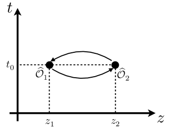
Figure 2: Counterclockwise monodromy of two operators $\widehat{\mathcal{O}}^{\,}_{1}(t^{\,}_{0},z^{\,}_{1})$ and $\widehat{\mathcal{O}}^{\,}_{2}(t^{\,}_{0},z^{\,}_{2})$ in the complex plane. When the operators $\widehat{\mathcal{O}}^{\,}_{1}$ and $\widehat{\mathcal{O}}^{\,}_{2}$ are evaluated at equal times, their exchange is related to their monodromy in the complex plane, provided that the handedness of the monodromy is specified. In particular, when $\widehat{\mathcal{O}}^{\,}_{1}=\widehat{\mathcal{O}}^{\,}_{2}$, we adopt the convention that the (holomorphic) operator with the larger value of $z$ is passed counterclockwise around the operator with the smaller value of $z$, resulting in the factors of $\text{sgn}(z-z^{\prime})$ that appear in the exchange algebras for the primary operators in this section.

The equal-time algebra of two twist operators is more subtle. For any pair of wires $y$ and $y^{\prime}$, the OPE of two twist fields in the complex plane is given by (see, e.g., Ardonne and Sierra (2010))

$$\widehat{\sigma}^{\,}_{\mathrm{L},y}(v)\,\widehat{\sigma}^{\,}_{\mathrm{L},y^{\prime}}(v^{\prime})= \,\delta^{\,}_{y,y^{\prime}}\,\frac{C^{\mathbbm{1}}_{\sigma\sigma}}{(v-v^{\prime})^{1/8}}$$

$$+\delta^{\,}_{y,y^{\prime}}\,C^{\psi}_{\sigma\sigma}\,(v-v^{\prime})^{3/8}\,\psi^{\,}_{\mathrm{L},y}(v),$$ (37a)

$$\widehat{\sigma}^{\,}_{\mathrm{R},y}(\bar{v})\,\widehat{\sigma}^{\,}_{\mathrm{R},y^{\prime}}(\bar{v}^{\prime})= \,\delta^{\,}_{y,y^{\prime}}\,\frac{C^{\mathbbm{1}}_{\sigma\sigma}}{(\bar{v}-\bar{v}^{\prime})^{1/8}}$$

$$\,+\delta^{\,}_{y,y^{\prime}}\,C^{\psi}_{\sigma\sigma}\,(\bar{v}-\bar{v}^{\prime})^{3/8}\,\psi^{\,}_{\mathrm{R},y}(\bar{v}),$$ (37b)

$$\widehat{\sigma}^{\,}_{\mathrm{L},y}(v)\,\widehat{\sigma}^{\,}_{\mathrm{R},y^{\prime}}(\bar{v}^{\prime})= \,\widehat{\sigma}^{\,}_{\mathrm{R},y}(\bar{v})\,\widehat{\sigma}^{\,}_{\mathrm{L},y^{\prime}}(v^{\prime})=0+\cdots.$$ (37c)

Since there are two singular terms appearing on the right-hand side of Eqs. (37a) and (37b), the product of two chiral twist fields must be defined with care. In particular, correlation functions involving multiple chiral twist fields are not well-defined unless the fusion channel $\mathbbm{1}$ or $\psi$ is specified Fendley et al. (2007). We choose an equal-time operator algebra that reflects this ambiguity in the definition of chiral correlation functions involving the twist field. Thus, we define the equal-time algebra

$$\widehat{\sigma}^{\,}_{\mathrm{L},y}(t,z)\,\widehat{\sigma}^{\,}_{\mathrm{L},y^{\prime}}(t,z^{\prime})=\widehat{\sigma}^{\,}_{\mathrm{L},y^{\prime}}(t,z^{\prime})\,\widehat{\sigma}^{\,}_{\mathrm{L},y}(t,z)$$

$$\qquad\times\begin{cases}e^{-\mathrm{i}\,\frac{\pi}{8}\,\delta^{\,}_{y,y^{\prime}}\,\mathrm{sgn}(z-z^{\prime})},&\mathrm{if}\ \sigma\times\sigma=\mathbbm{1},\\ e^{+\mathrm{i}\,\frac{3\pi}{8}\,\delta^{\,}_{y,y^{\prime}}\,\mathrm{sgn}(z-z^{\prime})},&\mathrm{if}\ \sigma\times\sigma=\psi,\end{cases}$$ (38a)

$$\widehat{\sigma}^{\,}_{\mathrm{R},y}(t,z)\,\widehat{\sigma}^{\,}_{\mathrm{R},y^{\prime}}(t,z^{\prime})=\widehat{\sigma}^{\,}_{\mathrm{R},y^{\prime}}(t,z^{\prime})\,\widehat{\sigma}^{\,}_{\mathrm{R},y}(t,z)$$

$$\qquad\times\begin{cases}e^{+\mathrm{i}\,\frac{\pi}{8}\,\delta^{\,}_{y,y^{\prime}}\,\mathrm{sgn}(z-z^{\prime})},&\mathrm{if}\ \sigma\times\sigma=\mathbbm{1},\\ e^{-\mathrm{i}\,\frac{3\pi}{8}\,\delta^{\,}_{y,y^{\prime}}\,\mathrm{sgn}(z-z^{\prime})},&\mathrm{if}\ \sigma\times\sigma=\psi,\end{cases}$$ (38b)

$$\widehat{\sigma}^{\,}_{\mathrm{L},y}(t,z)\,\widehat{\sigma}^{\,}_{\mathrm{R},y^{\prime}}(t,z^{\prime})=\widehat{\sigma}^{\,}_{\mathrm{R},y^{\prime}}(t,z^{\prime})\,\widehat{\sigma}^{\,}_{\mathrm{L},y}(t,z),$$ (38c)

in two-dimensional Minkowski space for any pair of wires $y$ and $y^{\prime}$ and for any $z\neq z^{\prime}$. We have used the shorthand notation $\sigma\times\sigma=\mathbbm{1}$ and $\sigma\times\sigma=\psi$ to distinguish the two possible fusion outcomes. The appearance of the phases $\pm\pi/8$ and $\mp 3\pi/8$ (and the correlation between their signs) is fixed by the OPE (37a) and (37b) and the fusion channel $\mathbbm{1}$ or $\mathbbm{\psi}$, and the sign $\mathrm{sgn}(z-z^{\prime})$ is used to keep track of the handedness of the exchange. The choice of the overall sign convention for the angles $\pm\pi/8$ and $\mp 3\pi/8$ is equivalent to a choice of analytic continuation into the complex plane in order to regularize the equal-time exchange of the two operators. It is important to stress here that this equal-time algebra is not well-defined unless one specifies a fusion channel. This ambiguity is essential. Its origin is physical, and it reflects the non-Abelian nature of the twist field. We will see in the next section that this ambiguity has important consequences for the topological degeneracy.

III.3.3 String operators and topological degeneracy on the two-torus

We shall consider two distinct wires $y$ and $y^{\prime}$ and a coordinate $z$ along any one of these wires. Periodic boundary conditions are imposed both along the $y$-direction and along the $z$-direction. Hence, the one-dimensional array of wires has the topology of a torus.

We are going to construct the equal-time algebra

$$\left\{\widehat{\Gamma}^{(\frac{1}{2})}_{1},\widehat{\Gamma}^{(1)}_{2}\right\}=0$$ (39)

for a first pair of nonlocal operators $\widehat{\Gamma}^{(\frac{1}{2})}_{1}$ and $\widehat{\Gamma}^{(1)}_{2}$. This pair will be shown to commute with the interaction (19). The nonlocal operator $\widehat{\Gamma}^{(\frac{1}{2})}_{1}$ can be thought of as creating a pair of pointlike “spin-$1/2$” excitations, transporting them in opposite directions around a noncontractible cycle of the torus along the $y$-direction, and then annihilating them. Likewise, the nonlocal operator $\widehat{\Gamma}^{(1)}_{2}$ can be thought of as implementing a similar process for a pair of pointlike “spin-$1$” excitations around a noncontractible cycle of the torus along the $z$-direction.

Similarly, we are going to construct the equal-time algebra

$$\left\{\widehat{\Gamma}^{(1)}_{1},\widehat{\Gamma}^{(\frac{1}{2})}_{2}\right\}=0$$ (40)

for a second pair of nonlocal operators $\widehat{\Gamma}^{(1)}_{1}$ and $\widehat{\Gamma}^{(\frac{1}{2})}_{2}$. This pair will also be shown to commute with the interaction (19), modulo appropriate regularization of the operator $\widehat{\Gamma}^{(\frac{1}{2})}_{2}$, as we will discuss. The nonlocal operator $\widehat{\Gamma}^{(1)}_{1}$ can be thought of as creating a pair of “spin-$1$” excitations, transporting them in opposite directions around a noncontractible cycle of the torus along the $y$-direction, and then annihilating them. The nonlocal operator $\widehat{\Gamma}^{(\frac{1}{2})}_{2}$ can be thought of as implementing the same process for a pair of “spin-$1/2$” excitations around a noncontractible cycle of the torus along the $z$-direction.

If we denote a ground state of the interaction (19) by $|\Omega\rangle$, we shall demonstrate that the three states

$$|\Omega\rangle,\quad\ket{\widehat{\Gamma}^{(\frac{1}{2})}_{1}}\,\raisebox{0.85pt}{.}\raisebox{2.85pt}{.}\!\!=\,\widehat{\Gamma}^{(\frac{1}{2})}_{1}\,|\Omega\rangle,\quad \ket{\widehat{\Gamma}^{(\frac{1}{2})}_{2}}\,\raisebox{0.85pt}{.}\raisebox{2.85pt}{.}\!\!=\,\widehat{\Gamma}^{(\frac{1}{2})}_{2}\,|\Omega\rangle,$$ (41)

are linearly independent ground states of the interaction (19). The proof of this claim relies on the vanishing equal-time commutators

$$\left[\widehat{\Gamma}^{(1)}_{2},\widehat{\Gamma}^{(1)}_{1}\right]=0,$$ (42)

$$\left[\widehat{\Gamma}^{(\frac{1}{2})}_{1},\widehat{\Gamma}^{(1)}_{1}\right]=0,$$ (43)

and

$$\left[\widehat{\Gamma}^{(1)}_{2},\widehat{\Gamma}^{(\frac{1}{2})}_{2}\right]=0.$$ (44)

Crucially, however, the exchange algebra of the nonlocal operators $\widehat{\Gamma}^{(\frac{1}{2})}_{1}$ and $\widehat{\Gamma}^{(\frac{1}{2})}_{2}$ suffers from the same ambiguity as that found on the right-hand side of Eq. (38). This is why one cannot infer from Eqs. (39)–(44) that the state

$$\widehat{\Gamma}^{(\frac{1}{2})}_{1}\,\widehat{\Gamma}^{(\frac{1}{2})}_{2}\,|\Omega\rangle$$ (45)

is linearly independent from the states (41). (See also Appendix B.)

Proof.

The proof consists of three steps.

Step 1: “Spin-$1$” string operators. The first string operators that we will construct are the “spin-$1$” string operators. We begin with strings running along the $y$-direction, perpendicular to the wires. These strings are built from the local bilinears

$$\begin{split}\widehat{\mathcal{O}}^{(1)}_{y}(t,z)\propto&\,\widehat{\Upsilon}^{(1)\dagger}_{\mathrm{L},y}(t,z)\,\widehat{\Upsilon}^{(1)}_{\mathrm{R},y}(t,z)\\ \propto&\,e^{-\mathrm{i}\frac{1}{\sqrt{2}}\widehat{\phi}^{\,}_{\mathrm{L},y}(t,z)}\,e^{+\mathrm{i}\frac{1}{\sqrt{2}}\widehat{\phi}^{\,}_{\mathrm{R},y}(t,z)},\end{split}$$ (46)

for any $0<z<L^{\,}_{z}$ (hereafter, we suppress the normal ordering of the vertex operators). The constants of proportionality omitted above appear in Sec. III.3.4, and are necessary for the proper normalization of these operators. Using Eq. (16d) for $k=2$, we see that a product of “spin-$1$” bilinears in neighboring wires commutes with the part of the interaction (19) that connects the two wires, since

$$\widehat{\mathcal{O}}^{(1)}_{y}(t,z)\,\widehat{\mathcal{O}}^{(1)}_{y+1}(t,z)\,e^{+\mathrm{i}\sqrt{1/2}\,\left[\widehat{\phi}^{\,}_{\mathrm{L},y}(t,z^{\prime})-\widehat{\phi}^{\,}_{\mathrm{R},y+1}(t,z^{\prime})\right]}=e^{+\mathrm{i}\sqrt{1/2}\,\left[\widehat{\phi}^{\,}_{\mathrm{L},y}(t,z^{\prime})-\widehat{\phi}^{\,}_{\mathrm{R},y+1}(t,z^{\prime})\right]}\,\widehat{\mathcal{O}}^{(1)}_{y}(t,z)\,\widehat{\mathcal{O}}^{(1)}_{y+1}(t,z),$$ (47)

and because $\widehat{\mathcal{O}}^{(1)}_{y}(t,z)$ commutes with any operator from the $\mathbb{Z}^{\,}_{2}$ sector of the theory. Thus, the nonlocal string operator

$$\widehat{\Gamma}^{(1)}_{1}(t,z)\,\raisebox{0.85pt}{.}\raisebox{2.85pt}{.}\!\!=\,\prod_{y=0}^{L^{\,}_{y}}\widehat{\mathcal{O}}^{(1)}_{y}(t,z)$$ (48)

commutes with the interaction (19) for any value of $0\leq z<L^{\,}_{z}$ when periodic boundary conditions are imposed in the $y$-direction. The nonlocal operator (48) is a member of the family

$$\widehat{\Gamma}^{(1)}_{1}(t,z^{\,}_{1},\cdots z^{\,}_{L^{\,}_{y}})\,\raisebox{0.85pt}{.}\raisebox{2.85pt}{.}\!\!=\,\widehat{\Upsilon}^{(1)\dagger}_{\mathrm{L},1}(t,z^{\,}_{1})\,\widehat{\Upsilon}^{(1)}_{\mathrm{R},1}(t,z^{\,}_{2})\,\widehat{\Upsilon}^{(1)\dagger}_{\mathrm{L},2}(t,z^{\,}_{2})\,\widehat{\Upsilon}^{(1)}_{\mathrm{R},2}(t,z^{\,}_{3})\,\cdots\,\widehat{\Upsilon}^{(1)\dagger}_{\mathrm{L},L^{\,}_{y}}(t,z^{\,}_{L^{\,}_{y}})\,\widehat{\Upsilon}^{(1)}_{\mathrm{R},L^{\,}_{y}}(t,z^{\,}_{1})$$ (49)

of operators, which all commute with the Hamiltonian defined by Eq. (13) for any values of $0\leq z^{\,}_{1},\cdots,z^{\,}_{L^{\,}_{y}}<L^{\,}_{z}$ when periodic boundary conditions are imposed in the $y$-direction. Any “spin-$1$” string operator from the family (49) can be viewed as creating a pair of “spin-$1$” excitations and transporting one of them around a noncontractible loop that encircles the torus in the $y$-direction (a noncontractible cycle along the $y$-direction), before annihilating it with its partner.

To construct a “spin-$1$” string running along the $z$-direction, parallel to the wires, we consider the operator

$$\begin{split}&\widehat{\mathcal{O}}^{(1)}_{\mathrm{M},y}(t,z^{\,}_{1},z^{\,}_{2})\propto\widehat{\Upsilon}^{(1)\dagger}_{\mathrm{M},y}(t,z^{\,}_{2})\,\widehat{\Upsilon}^{(1)}_{\mathrm{M},y}(t,z^{\,}_{1})\\ &\qquad\propto\exp\Bigg{(}-\mathrm{i}\frac{1}{\sqrt{2}}\int\limits^{z^{\,}_{2}}_{z^{\,}_{1}}\mathrm{d}z\,\partial^{\,}_{z}\widehat{\phi}^{\,}_{\mathrm{M},y}(t,z)\Bigg{)}\end{split}$$ (50a)

for any $$0\leq z^{\,}_{1},z^{\,}_{2}<L^{\,}_{z} \mathrm{M}=\mathrm{L},\mathrm{R}$$ and .

Hence, $\widehat{\mathcal{O}}^{(1)}_{\mathrm{M},y}(t,z^{\,}_{1},z^{\,}_{2})$ is a bilocal operator that also obeys

$$\widehat{\mathcal{O}}^{(1)}_{\mathrm{L},y}(t,z^{\,}_{1},z^{\,}_{2})\,e^{+\mathrm{i}\sqrt{1/2}\,\left[\widehat{\phi}^{\,}_{\mathrm{L},y}(t,z)-\widehat{\phi}^{\,}_{\mathrm{R},y+1}(t,z)\right]}= \,e^{+\mathrm{i}\sqrt{1/2}\,\left[\widehat{\phi}^{\,}_{\mathrm{L},y}(t,z)-\widehat{\phi}^{\,}_{\mathrm{R},y+1}(t,z)\right]}\,\widehat{\mathcal{O}}^{(1)}_{\mathrm{L},y}(t,z^{\,}_{1},z^{\,}_{2})\times e^{+\mathrm{i}2\pi\int\limits^{z^{\,}_{2}}_{z^{\,}_{1}}\mathrm{d}z^{\prime}\,\delta(z-z^{\prime})},$$ (51)

as a result of Eq. (16d) for $k=2$. (A similar expression holds for $\mathrm{M}=\mathrm{R}$.) Now define the nonlocal operator

$$\widehat{\Gamma}^{(1)}_{2,\mathrm{M},y}(t)\propto\widehat{\mathcal{O}}^{(1)}_{\mathrm{M},y}(t,0,L^{\,}_{z}),$$ (52)

which commutes with the interaction (19) by Eq. (51). This “spin-$1$” string operator can be viewed as transporting a “spin-$1$” excitation around a noncontractible loop that encircles the torus in the $z$-direction (a noncontractible cycle along the $z$-direction).

The equal-time commutation relation between the string operators (48) with $0<z<L^{\,}_{z}$ and (52) is computed using Eq. (16d) for $k=2$. It is simply the commutative rule

$$\widehat{\Gamma}^{(1)}_{1}(t,z)\,\widehat{\Gamma}^{(1)}_{2,\mathrm{M},y}(t)= \,\widehat{\Gamma}^{(1)}_{2,\mathrm{M},y}(t)\,\widehat{\Gamma}^{(1)}_{1}(t,z),$$ (53)

for any $\mathrm{M}=\mathrm{L},\mathrm{R}$. This result reflects the fact that the spin-1 primary operator in the $su(2)^{\,}_{2}$ has trivial self-monodromy. We have established Eq. (42) provided we make the identifications

$$\widehat{\Gamma}^{(1)}_{1}(t,z)\to\widehat{\Gamma}^{(1)}_{1},\quad\mathrm{and}\quad\widehat{\Gamma}^{(1)}_{2,\mathrm{M},y}(t)\to\widehat{\Gamma}^{(1)}_{2},$$ (54)

for some choice of chirality $\mathrm{M}$ and wire $y$.

Step 2: “Spin-$1/2$” string operators. We next construct string operators associated with the spin-$1/2$ primary of the $su(2)^{\,}_{k}$ theory. We proceed according to a strategy similar to the one used for the “spin-$1$” strings. To construct a “spin-$1/2$” string along the $y$-direction, let $0<z,z^{\prime}<L^{\,}_{z}$ and consider the local “spin-$1/2$” bilinears

$$\widehat{\mathcal{O}}^{(\frac{1}{2})}_{y}(t,z) \propto\widehat{\Upsilon}^{(\frac{1}{2})\dagger}_{\mathrm{L},y}(t,z)\,\widehat{\Upsilon}^{(\frac{1}{2})}_{\mathrm{R},y}(t,z)$$

$$\propto e^{-\mathrm{i}\frac{1}{2\sqrt{2}}\widehat{\phi}^{\,}_{\mathrm{L},y}(t,z)}e^{+\mathrm{i}\frac{1}{2\sqrt{2}}\widehat{\phi}^{\,}_{\mathrm{R},y}(t,z)}$$ (55a)

$$\qquad\times\widehat{\sigma}^{\,}_{\mathrm{L},y}(t,z)\,\widehat{\sigma}^{\,}_{\mathrm{R},y}(t,z),$$

where we have defined the operator

$$\widehat{\Upsilon}^{(\frac{1}{2})\dagger}_{\mathrm{L},y}(t,z)\,\raisebox{0.85pt}{.}\raisebox{2.85pt}{.}\!\!=\,e^{-\mathrm{i}\frac{1}{2\sqrt{2}}\widehat{\phi}^{\,}_{\mathrm{L},y}(t,z)}\,\widehat{\sigma}^{\,}_{\mathrm{L},y}(t,z),$$ (55b)

in which the adjoint operation pertains only to the $u(1)^{\,}_{k}$ vertex operator. Using Eqs. (16d) and (36), we find that the equal-time product of such bilinears over all wires, namely

$$\widehat{\Gamma}^{(\frac{1}{2})}_{1}(t,z)\,\raisebox{0.85pt}{.}\raisebox{2.85pt}{.}\!\!=\,\prod_{y=0}^{L^{\,}_{y}}\widehat{\mathcal{O}}^{(\frac{1}{2})}_{y}(t,z),$$ (56)

commutes with the interaction (19) for any value $0<z<L^{\,}_{z}$ when periodic boundary conditions are imposed in the $y$-direction. This nonlocal operator is a member of the family

$$\widehat{\Gamma}^{(\frac{1}{2})}_{1}(t,z^{\,}_{1},\cdots,z^{\,}_{L^{\,}_{y}})\,\raisebox{0.85pt}{.}\raisebox{2.85pt}{.}\!\!=\,\widehat{\Upsilon}^{(\frac{1}{2})\dagger}_{\mathrm{L},1}(t,z^{\,}_{1})\,\widehat{\Upsilon}^{(\frac{1}{2})}_{\mathrm{R},1}(t,z^{\,}_{2})\,\widehat{\Upsilon}^{(\frac{1}{2})\dagger}_{\mathrm{L},2}(t,z^{\,}_{2})\,\widehat{\Upsilon}^{(\frac{1}{2})}_{\mathrm{R},2}(t,z^{\,}_{3})\,\cdots\,\widehat{\Upsilon}^{(\frac{1}{2})\dagger}_{\mathrm{L},L^{\,}_{y}}(t,z^{\,}_{L^{\,}_{y}})\,\widehat{\Upsilon}^{(\frac{1}{2})}_{\mathrm{R},L^{\,}_{y}}(t,z^{\,}_{1})$$ (57)

of operators that commute with the Hamiltonian defined by Eq. (13) for any values of $0<z^{\,}_{1},\cdots,z^{\,}_{L^{\,}_{y}}<L^{\,}_{z}$ when periodic boundary conditions are imposed in the $y$-direction. Any “spin-$1/2$” string operator from the family (57) can be interpreted as creating a pair of “spin-$1/2$” excitations and transporting one of them around a noncontractible cycle along the $y$-direction, before annihilating it with its partner.

We first observe that the operators $\widehat{\Gamma}^{(1)}_{1}(t,z)$ and $\widehat{\Gamma}^{(\frac{1}{2})}_{1}(t,z^{\prime})$ commute with one another for any $z$ and $z^{\prime}$, as one can show using the equal-time algebra (16d),

$$\widehat{\Gamma}^{(1)}_{1}(t,z)\,\widehat{\Gamma}^{(\frac{1}{2})}_{1}(t,z^{\prime})=\widehat{\Gamma}^{(\frac{1}{2})}_{1}(t,z^{\prime})\,\widehat{\Gamma}^{(1)}_{1}(t,z).$$ (58)

We have established Eq. (43) provided we make the identifications

$$\widehat{\Gamma}^{(1)}_{1}(t,z)\to\widehat{\Gamma}^{(1)}_{1},\qquad\widehat{\Gamma}^{(\frac{1}{2})}_{1}(t,z^{\prime})\to\widehat{\Gamma}^{(\frac{1}{2})}_{1}.$$ (59)

We claim that the “spin-$1/2$” string $\widehat{\Gamma}^{(\frac{1}{2})}_{1}$ can be interpreted as an operator that “twists,” from antiperiodic to periodic, the boundary conditions of a “spin-$1$” excitation that encircles the torus in the $z$-direction. To see that this is the case, we use the chiral boson algebra of Eq. (16d) to show that the equal-time operator algebra

$$\widehat{\Gamma}^{(1)}_{2,\mathrm{M},y}(t)\,\widehat{\Gamma}^{(\frac{1}{2})}_{1}(t,z)= \,-\widehat{\Gamma}^{(\frac{1}{2})}_{1}(t,z)\,\widehat{\Gamma}^{(1)}_{2,\mathrm{M},y}(t)$$ (60)

holds for any choice of chirality $\mathrm{M}=\mathrm{L},\mathrm{R}$ and wire $y$. We further recall that the operator $\widehat{\Gamma}^{(1)}_{2,\mathrm{M},y}(t)$ transports a “spin-$1$” excitation around the torus along the $z$-direction. Thus, Eq. (60) shows that the amplitude for transporting a “spin-$1$” excitation around the torus and then applying the operator $\widehat{\Gamma}^{(\frac{1}{2})}_{1}(t,z)$ differs by a minus sign from the amplitude for applying the operator $\widehat{\Gamma}^{(\frac{1}{2})}_{1}(t,z)$ and then transporting a “spin-$1$” excitation around the torus. This is precisely the action of an operator that twists the boundary conditions of a“spin-$1$” excitation.

In deriving Eq. (60), we have established Eq. (39) provided that we make the identifications

$$\widehat{\Gamma}^{(1)}_{2,\mathrm{M},y}(t)\to\widehat{\Gamma}^{(1)}_{2},\qquad\widehat{\Gamma}^{(\frac{1}{2})}_{1}(t,z)\to\widehat{\Gamma}^{(\frac{1}{2})}_{1}.$$ (61)

for some choice of chirality $\mathrm{M}$ and wire $y$.

Next, we seek an operator that twists the boundary conditions of a “spin-$1$” excitation encircling the torus along the $y$-direction. We proceed in direct analogy with Eq. (50a) by defining the (nonlocal ) operator

$$\widehat{\mathcal{O}}^{(\frac{1}{2})}_{\mathrm{M},y^{\prime}}(t,z^{\,}_{1},z^{\,}_{2}) \propto\widehat{\Upsilon}^{(\frac{1}{2})\dagger}_{\mathrm{M},y^{\prime}}(t,z^{\,}_{2})\,\widehat{\Upsilon}^{(\frac{1}{2})}_{\mathrm{M},y^{\prime}}(t,z^{\,}_{1})$$

$$\propto\exp\Bigg{(}-\mathrm{i}\frac{1}{2\sqrt{2}}\int\limits^{z^{\,}_{2}}_{z^{\,}_{1}}\mathrm{d}z\,\partial^{\,}_{z}\widehat{\phi}^{\,}_{\mathrm{M},y^{\prime}}(t,z)\Bigg{)}$$

$$\qquad\times\widehat{\sigma}^{\,}_{\mathrm{M},y^{\prime}}(t,z^{\,}_{2})\,\widehat{\sigma}^{\,}_{\mathrm{M},y^{\prime}}(t,z^{\,}_{1}).$$ (62)

We seek to define a string operator by taking $z^{\,}_{1}\to 0$ and $z^{\,}_{2}\to L^{\,}_{z}$. However, one must be careful in taking these limits since Eq. (62) contains two chiral $\mathbb{Z}^{\,}_{2}$ twist fields in the same wire. Due to the ambiguity of the OPE (38), such a product is ill-defined unless a fusion channel is specified. [Meanwhile, the product of $u(1)^{\,}_{2}$ vertex operators is unambiguous.] By analogy with the construction of $\widehat{\Gamma}^{(1)}_{2}$ in Eq. (50a), we would like to define the string operator $\widehat{\Gamma}^{(\frac{1}{2})}_{2}$ in such a way as to leave the system in the vacuum sector. Hence, the natural choice is to specify that the two $\widehat{\sigma}^{\,}_{M,y^{\prime}}$ operators in Eq. (62) fuse to the identity operator $\mathbbm{1}$. In addition to providing a sensible parallel with the construction of $\widehat{\Gamma}^{(1)}_{1}$, this choice agrees with the choice made in the construction of the operator that tunnels an $e/4$ quasiparticle across a quantum point contact in the Moore-Read state Fendley et al. (2007).

This motivates the definition of the “spin-$1/2$” string operator

$$\begin{split}\widehat{\Gamma}^{(\frac{1}{2})}_{2,\mathrm{M},y^{\prime}}(t,\epsilon)&\,\raisebox{0.85pt}{.}\raisebox{2.85pt}{.}\!\!=\,\exp\Bigg{(}-\mathrm{i}\frac{1}{2\sqrt{2}}\int\limits^{L^{\,}_{z}}_{0}\mathrm{d}z\,\partial^{\,}_{z}\widehat{\phi}^{\,}_{\mathrm{M},y^{\prime}}(t,z)\Bigg{)}\\ &\qquad\times\widehat{\mathcal{P}}^{\,}_{\mathbbm{1}}\,\widehat{\sigma}^{\,}_{\mathrm{M},y^{\prime}}(t,0)\,\widehat{\sigma}^{\,}_{\mathrm{M},y^{\prime}}(t,\epsilon)\,\widehat{\mathcal{P}}^{\,}_{\mathbbm{1}},\end{split}$$ (63)

where $\widehat{\mathcal{P}}^{\,}_{\mathbbm{1}}$ is the projection operator onto the fusion channel $\sigma\times\sigma=\mathbbm{1}$. (This projection can also be implemented by an appropriate choice of normalization, as is done in Sec. III.3.4.) One can show that this projector does not affect the algebra of twist operators $\widehat{\sigma}^{\,}_{\mathrm{M},y}$ and Majorana operators $\widehat{\psi}^{\,}_{\mathrm{M},y}$. We claim that the string operator $\widehat{\Gamma}^{(\frac{1}{2})}_{2,\mathrm{M},y^{\prime}}(t,\epsilon)$ defined in this way commutes with the interaction (19) in the limit $\epsilon\to 0$. To see this, note that

$$\lim_{\epsilon\to 0}\widehat{\psi}^{\,}_{\mathrm{L},y}(t,z)\,\widehat{\psi}^{\,}_{\mathrm{R},y+1}(t,z)\,\widehat{\sigma}^{\,}_{\mathrm{L},y^{\prime}}(t,0)\,\widehat{\sigma}^{\,}_{\mathrm{L},y^{\prime}}(t,\epsilon)=\lim_{\epsilon\to 0}\widehat{\sigma}^{\,}_{\mathrm{L},y^{\prime}}(t,0)\,\widehat{\sigma}^{\,}_{\mathrm{L},y^{\prime}}(t,\epsilon)\,\widehat{\psi}^{\,}_{\mathrm{L},y}(t,z)\,\widehat{\psi}^{\,}_{\mathrm{R},y+1}(t,z)\times\begin{cases}+1,&y\neq y^{\prime},\\ -1,&y=y^{\prime},\end{cases}$$ (64)

follows from the algebra (36), while

$$\begin{split}&e^{+\mathrm{i}\sqrt{1/2}\,\left[\widehat{\phi}^{\,}_{\mathrm{L},y}(t,z)-\widehat{\phi}^{\,}_{\mathrm{R},y+1}(t,z)\right]}\,\exp\Bigg{(}-\mathrm{i}\frac{1}{2\sqrt{2}}\int\limits^{L^{\,}_{z}}_{0}\mathrm{d}z\,\partial^{\,}_{z}\widehat{\phi}^{\,}_{\mathrm{L},y^{\prime}}(t,z)\Bigg{)}\\ &\qquad\qquad\qquad=\exp\Bigg{(}-\mathrm{i}\frac{1}{2\sqrt{2}}\int\limits^{L^{\,}_{z}}_{0}\mathrm{d}z\,\partial^{\,}_{z}\widehat{\phi}^{\,}_{\mathrm{L},y^{\prime}}(t,z)\Bigg{)}\,e^{+\mathrm{i}\sqrt{1/2}\,\left[\widehat{\phi}^{\,}_{\mathrm{L},y}(t,z)-\widehat{\phi}^{\,}_{\mathrm{R},y+1}(t,z)\right]}\times\begin{cases}+1,&y\neq y^{\prime},\\ -1,&y=y^{\prime},\end{cases}\end{split}$$ (65)

follows from the algebra (16d). (Similar expressions hold for $\mathrm{M}=\mathrm{R}$.) Consequently, $\widehat{\Gamma}^{(\frac{1}{2})}_{2,\mathrm{M},y^{\prime}}(t,\epsilon)$ commutes with the interaction (19) in the limit $\epsilon\to 0$ foo .

Moreover, we can also show that $\widehat{\Gamma}^{(\frac{1}{2})}_{2,\mathrm{M},y^{\prime}}(t,\epsilon)$ twists the boundary conditions of a “spin-$1$” excitation encircling the torus along the $y$-direction. To do this, we use the algebra (16d) to compute the exchange relation (in the limit $\epsilon\to 0$)

$$\widehat{\Gamma}^{(\frac{1}{2})}_{2,\mathrm{M},y^{\prime}}(t,\epsilon)\,\widehat{\Gamma}^{(1)}_{1}(t,z)\,= \,-\widehat{\Gamma}^{(1)}_{1}(t,z)\,\widehat{\Gamma}^{(\frac{1}{2})}_{2,\mathrm{M},y^{\prime}}(t,\epsilon),$$ (66)

which holds for any chirality $\mathrm{M}$ and wire $y^{\prime}$. This exchange relation has an interpretation similar to Eq. (60). Thus, we have established Eq. (40) provided we make the identifications

$$\widehat{\Gamma}^{(1)}_{1}(t,z)\to\widehat{\Gamma}^{(1)}_{1},\qquad\widehat{\Gamma}^{(\frac{1}{2})}_{2,\mathrm{M},y^{\prime}}(t,\epsilon)\to\widehat{\Gamma}^{(\frac{1}{2})}_{2},$$ (67)

for infinitesimal $\epsilon>0$. By assumption $y\neq y^{\prime}$. Hence, the operators $\widehat{\Gamma}^{\psi}_{2,y}\to\widehat{\Gamma}^{(1)}_{2}$ and $\widehat{\Gamma}^{\sigma}_{2,\mathrm{M},y^{\prime}}\to\widehat{\Gamma}^{(\frac{1}{2})}_{2}$ commute with one another in a trivial way. This establishes Eq. (44).

Step 3: The topological degeneracy. There exists a many-body ground state

$$\ket{\Omega}\equiv\ket{\mathbbm{1}}$$ (68a)

of the interaction $$\widehat{\mathcal{H}}^{\,}_{\mathrm{bs}} 1/2 y z$$ defined in Eq. (19) from which we can obtain two additional many-body states by acting with the “spin-” string operators along the - and -directions, respectively,

$$\ket{\widehat{\Gamma}^{(\frac{1}{2})}_{1}}\,\raisebox{0.85pt}{.}\raisebox{2.85pt}{.}\!\!=\,\widehat{\Gamma}^{(\frac{1}{2})}_{1}(t,z)\ket{\Omega}$$ (68b)

and

$$\ket{\widehat{\Gamma}^{(\frac{1}{2})}_{2}}\,\raisebox{0.85pt}{.}\raisebox{2.85pt}{.}\!\!=\,\lim_{\epsilon\to 0}\widehat{\Gamma}^{(\frac{1}{2})}_{2,\mathrm{R},y^{\prime}}(t,\epsilon)\ket{\Omega},$$ (68c)

for any $z$, $y^{\prime}$, and $z^{\,}_{1}$. It is important to point out that not all choices of $\ket{\Omega}$ are equal. As argued in Appendix B, depending on the topological sector in which the state $\ket{\Omega}$ resides, one or both of the states (68b) and (68c) could have norm zero or infinity. We will first prove that the many-body states $\ket{\widehat{\Gamma}^{(\frac{1}{2})}_{1}}$ and $\ket{\widehat{\Gamma}^{(\frac{1}{2})}_{2}}$ share the same eigenvalue of $\widehat{\mathcal{H}}^{\,}_{\mathrm{bs}}$ as $\ket{\Omega}$. Second, we will prove that the many-body states (68) are linearly independent. In doing so, we will have established that the ground state degeneracy on the torus of the interaction $\widehat{\mathcal{H}}^{\,}_{\mathrm{bs}}$ is threefold.

First, we recall that $\widehat{\Gamma}^{(\frac{1}{2})}_{1}(t,z)$ commutes with the interaction $\widehat{\mathcal{H}}^{\,}_{\mathrm{bs}}$ defined in Eq. (19). Hence, the many-body state $\ket{\widehat{\Gamma}^{(\frac{1}{2})}_{1}}$ defined in Eq. (68b) is a ground state of the interaction $\widehat{\mathcal{H}}^{\,}_{\mathrm{bs}}$. Making sure to treat the limit $\epsilon\to 0$ with care, we show in Appendix B that the many-body state $\ket{\widehat{\Gamma}^{(\frac{1}{2})}_{2}}$ defined in Eq. (68b) is also a ground state of the interaction $\widehat{\mathcal{H}}^{\,}_{\mathrm{bs}}$. Now, we are going to show that the three many-body states (68) are linearly independent.

The operators $\widehat{\Gamma}^{(1)}_{1}$ and $\widehat{\Gamma}^{(1)}_{2}$ commute with the interaction $\widehat{\mathcal{H}}^{\,}_{\mathrm{bs}}$ and with each other [recall Eq. (42)]. They are thus simultaneously diagonalizable. Consequently, we can choose $\ket{\Omega}$ to be a simultaneous eigenstate of the pair of operators $\widehat{\Gamma}^{(1)}_{1}$ and $\widehat{\Gamma}^{(1)}_{2}$. We assume that $\widehat{\Gamma}^{(1)}_{1}$ and $\widehat{\Gamma}^{(1)}_{2}$ have the unimodular eigenvalues $\omega^{(1)}_{1}\neq 0$ and $\omega^{(1)}_{2}\neq 0$ such that

$$\widehat{\Gamma}^{(1)}_{1}\,\ket{\Omega}=\omega^{(1)}_{1}\,\ket{\Omega},$$ (69a)

and

$$\widehat{\Gamma}^{(1)}_{2}\,\ket{\Omega}=\omega^{(1)}_{2}\,\ket{\Omega},$$ (69b)

respectively.

Because of the anticommutator (39), we find the eigenvalue

$$\widehat{\Gamma}^{(1)}_{2}\,\ket{\widehat{\Gamma}^{(\frac{1}{2})}_{1}}=-\omega^{(1)}_{2}\,\ket{\widehat{\Gamma}^{(\frac{1}{2})}_{1}}.$$ (70)

Hence, $\ket{\Omega}$ and $\ket{\widehat{\Gamma}^{(\frac{1}{2})}_{1}}$ are simultaneous eigenstates of the operator $\Gamma^{(1)}_{2}$ with distinct eigenvalues. As such, $\ket{\Omega}$ and $\ket{\widehat{\Gamma}^{(\frac{1}{2})}_{1}}$ are othogonal. Similarly, because of the anticommutator (40), we find the eigenvalue

$$\widehat{\Gamma}^{(1)}_{1}\,\ket{\widehat{\Gamma}^{(\frac{1}{2})}_{2}}=-\omega^{(1)}_{1}\,\ket{\widehat{\Gamma}^{(\frac{1}{2})}_{2}}.$$ (71)

Hence, $\ket{\Omega}$ and $\ket{\widehat{\Gamma}^{(\frac{1}{2})}_{2}}$ are simultaneous eigenstates of the operator $\Gamma^{(1)}_{1}$ with distinct eigenvalues. As such, $\ket{\Omega}$ and $\ket{\widehat{\Gamma}^{(\frac{1}{2})}_{2}}$ are othogonal.

To complete the proof that $\ket{\Omega}$, $\ket{\widehat{\Gamma}^{(\frac{1}{2})}_{1}}$, and $\ket{\widehat{\Gamma}^{(\frac{1}{2})}_{2}}$ are linearly independent, it suffices to show that $\ket{\widehat{\Gamma}^{(\frac{1}{2})}_{1}}$ and $\ket{\widehat{\Gamma}^{(\frac{1}{2})}_{2}}$ are orthogonal. Because of the commutator (43), we find the eigenvalue

$$\widehat{\Gamma}^{(1)}_{1}\,\ket{\widehat{\Gamma}^{(\frac{1}{2})}_{1}}=+\omega^{(1)}_{1}\,\ket{\widehat{\Gamma}^{(\frac{1}{2})}_{1}}.$$ (72)

Hence, $\ket{\widehat{\Gamma}^{(\frac{1}{2})}_{1}}$ and $\ket{\widehat{\Gamma}^{(\frac{1}{2})}_{2}}$ are simultaneous eigenstates of the operator $\widehat{\Gamma}^{(1)}_{1}$ with the pair of distinct eigenvalues $+\omega^{(1)}_{1}$ and $-\omega^{(1)}_{1}$. As such, $\ket{\widehat{\Gamma}^{(\frac{1}{2})}_{1}}$ and $\ket{\widehat{\Gamma}^{(\frac{1}{2})}_{2}}$ are orthogonal.

We note that the commutator (44) could equally well have been used to show that $\ket{\widehat{\Gamma}^{(\frac{1}{2})}_{1}}$ and $\ket{\widehat{\Gamma}^{(\frac{1}{2})}_{2}}$ are simultaneous eigenstates of the operator $\widehat{\Gamma}^{(1)}_{2}$ with the pair of distinct eigenvalues $+\omega^{(1)}_{2}$ and $-\omega^{(1)}_{2}$.

As promised, we have shown that the ground-state manifold of the interaction $\widehat{\mathcal{H}}^{\,}_{\mathrm{bs}}$ on the torus is threefold degenerate.   $\ \square$

It is useful to pause at this stage to interpret this lower bound on the ground state degeneracy and how it comes about. Naively, given two pairs of anticommuting nonlocal operators, all of which commute with the Hamiltonian, [i.e., given Eqs. (39) and (40)] there are at most four degenerate ground states. In the case of Kitaev’s toric code Kitaev (2003), the dimensionality of the ground state manifold saturates this upper bound. However, in the case of the two-dimensional state of matter that we have constructed here, we argue that this is not the case. The reason for this is intimately related to the nonunitarity of the string operators $\widehat{\Gamma}^{(\frac{1}{2})}_{1}(t,z)$ and $\widehat{\Gamma}^{(\frac{1}{2})}_{2,\mathrm{R},y^{\prime}}(t,\epsilon)$.

In particular, we assert that neither of the naively-expected fourth states, namely

$$\ket{\widehat{\Gamma}^{(\frac{1}{2})}_{1}\,\widehat{\Gamma}^{(\frac{1}{2})}_{2}}\,\raisebox{0.85pt}{.}\raisebox{2.85pt}{.}\!\!=\,\lim_{\epsilon\to 0}\widehat{\Gamma}^{(\frac{1}{2})}_{1}(t,z)\,\widehat{\Gamma}^{(\frac{1}{2})}_{2,\mathrm{R},y^{\prime}}(t,\epsilon)\,\ket{\Omega},$$ (73a)

and

$$\ket{\widehat{\Gamma}^{(\frac{1}{2})}_{2}\,\widehat{\Gamma}^{(\frac{1}{2})}_{1}}\,\raisebox{0.85pt}{.}\raisebox{2.85pt}{.}\!\!=\,\lim_{\epsilon\to 0}\widehat{\Gamma}^{(\frac{1}{2})}_{2,\mathrm{R},y^{\prime}}(t,\epsilon)\,\widehat{\Gamma}^{(\frac{1}{2})}_{1}(t,z)\,\ket{\Omega},$$ (73b)

belongs to the ground-state manifold of the interaction $\widehat{\mathcal{H}}^{\,}_{\mathrm{bs}}$. Note that the limit $\epsilon\to 0$ above is to be taken after forming the products $\widehat{\Gamma}^{(\frac{1}{2})}_{1}(t,z)\,\widehat{\Gamma}^{(\frac{1}{2})}_{2,\mathrm{R},y^{\prime}}(t,\epsilon)$ and $\widehat{\Gamma}^{(\frac{1}{2})}_{2,\mathrm{R},y^{\prime}}(t,\epsilon)\,\widehat{\Gamma}^{(\frac{1}{2})}_{1}(t,z)$, as discussed in Footnote foo and Appendix B. If the operator products $\widehat{\Gamma}^{(\frac{1}{2})}_{1}(t,z)\,\widehat{\Gamma}^{(\frac{1}{2})}_{2,\mathrm{R},y^{\prime}}(t,\epsilon)$ and $\widehat{\Gamma}^{(\frac{1}{2})}_{2,\mathrm{R},y^{\prime}}(t,\epsilon)\,\widehat{\Gamma}^{(\frac{1}{2})}_{1}(t,z)$ were to commute with the interaction $\widehat{\mathcal{H}}^{\,}_{\mathrm{bs}}$ in the limit $\epsilon\to 0$, as they would in an Abelian topological phase, then there would be no obstruction to the states $\ket{\widehat{\Gamma}^{(\frac{1}{2})}_{1}\,\widehat{\Gamma}^{(\frac{1}{2})}_{2}}$ and $\ket{\widehat{\Gamma}^{(\frac{1}{2})}_{2}\,\widehat{\Gamma}^{(\frac{1}{2})}_{1}}$ belonging to the ground-state manifold. The proof that such an obstruction exists in the present (non-Abelian) case is undertaken in two complementary ways in the present work. The first, which we call the “algebraic” approach, relies on diagrammatic techniques developed in Appendix C, and is presented below. The second, which we call the “analytic” approach, is carried out in Appendix B. Both the “algebraic” and “analytic” proofs rely on the fact, discussed in Appendix B, that the operator products $\widehat{\Gamma}^{(\frac{1}{2})}_{1}(t,z)\,\widehat{\Gamma}^{(\frac{1}{2})}_{2,\mathrm{R},y^{\prime}}(t,\epsilon)$ and $\widehat{\Gamma}^{(\frac{1}{2})}_{2,\mathrm{R},y^{\prime}}(t,\epsilon)\,\widehat{\Gamma}^{(\frac{1}{2})}_{1}(t,z)$ are not bound to commute with the interaction $\widehat{\mathcal{H}}^{\,}_{\mathrm{bs}}$ in the limit $\epsilon\to 0$. We now proceed with the “algebraic” version of the proof, and refer the reader to Appendices C and B for more details.

Proof (“algebraic”).

We introduce the projection operator

$$\begin{split}\widehat{\mathcal{P}}^{\,}_{\rm{GSM}}\,\raisebox{0.85pt}{.}\raisebox{2.85pt}{.}\!\!=\,&\,\mathcal{N}^{-1}_{\mathbbm{1}}\,\ket{\mathbbm{1}}\bra{\mathbbm{1}}\\ &\,+\mathcal{N}^{-1}_{\widehat{\Gamma}^{(\frac{1}{2})}_{1}}\,\ket{\widehat{\Gamma}^{(\frac{1}{2})}_{1}}\bra{\widehat{\Gamma}^{(\frac{1}{2})}_{1}}\\ &\,+\mathcal{N}^{-1}_{\widehat{\Gamma}^{(\frac{1}{2})}_{2}}\,\ket{\widehat{\Gamma}^{(\frac{1}{2})}_{2}}\bra{\widehat{\Gamma}^{(\frac{1}{2})}_{2}}\\ &\,+\cdots\end{split}$$ (74)

onto the ground state manifold. Here, $\mathcal{N}^{\,}_{\mathbbm{1}}$ is the squared norm of the state $\ket{\mathbbm{1}}\equiv\ket{\Omega}$, $\mathcal{N}^{\,}_{\widehat{\Gamma}^{(\frac{1}{2})}_{1}}$ is the squared norm of the state $\ket{\widehat{\Gamma}^{(\frac{1}{2})}_{1}}$, $\mathcal{N}^{\,}_{\widehat{\Gamma}^{(\frac{1}{2})}_{2}}$ is the squared norm of the state $\ket{\widehat{\Gamma}^{(\frac{1}{2})}_{2}}$, and $\cdots$ is a sum over any remaining elements from the orthonormal basis of the ground state manifold. By definition, any one of the three states $\ket{\mathbbm{1}}$, $\ket{\widehat{\Gamma}^{(\frac{1}{2})}_{1}}$, and $\ket{\widehat{\Gamma}^{(\frac{1}{2})}_{2}}$ defined in Eq. (68) is invariant under the action of

$$\widehat{\mathcal{P}}^{\,}_{\mathrm{GSM}}=\widehat{\mathcal{P}}^{2}_{\mathrm{GSM}}.$$ (75)

Hence, we may write

$$\ket{\widehat{\Gamma}^{(\frac{1}{2})}_{1}}= \,\widehat{\mathcal{P}}^{\,}_{\mathrm{GSM}}\,\ket{\widehat{\Gamma}^{(\frac{1}{2})}_{1}}=\widehat{\mathcal{P}}^{\,}_{\mathrm{GSM}}\,\widehat{\Gamma}^{(\frac{1}{2})}_{1}(t,z)\,\widehat{\mathcal{P}}^{\,}_{\mathrm{GSM}}\,\ket{\Omega},$$ (76a)

$$\ket{\widehat{\Gamma}^{(\frac{1}{2})}_{2}}= \,\widehat{\mathcal{P}}^{\,}_{\mathrm{GSM}}\,\ket{\widehat{\Gamma}^{(\frac{1}{2})}_{2}}=\widehat{\mathcal{P}}^{\,}_{\mathrm{GSM}}\,\lim_{\epsilon\to 0}\widehat{\Gamma}^{(\frac{1}{2})}_{2,\mathrm{R},y^{\prime}}(t,\epsilon)\,\widehat{\mathcal{P}}^{\,}_{\mathrm{GSM}}\,\ket{\Omega}.$$ (76b)

On the other hand,

$$\widehat{\mathcal{P}}^{\,}_{\rm{GSM}}\,\widehat{\mathcal{O}}\,\widehat{\mathcal{P}}^{\,}_{\rm{GSM}}=0$$ (77)

must hold for any operator $\widehat{\mathcal{O}}$ such that $\widehat{\mathcal{O}}$ returns an excited state when applied to any state from the ground-state manifold.

We are first going to show that the operators $\widehat{\Gamma}^{(\frac{1}{2})}_{1}(t,z)$ and $\widehat{\Gamma}^{(\frac{1}{2})}_{2,\mathrm{R},y^{\prime}}(t,\epsilon)$ do not commute in the limit $\epsilon\to 0$. After that, we will elaborate on why the state $\ket{\widehat{\Gamma}^{(\frac{1}{2})}_{1}\,\widehat{\Gamma}^{(\frac{1}{2})}_{2}}$ does not belong to the ground-state manifold of the interaction $\widehat{\mathcal{H}}^{\,}_{\mathrm{bs}}$.

We begin by considering the exchange algebra of the string operators $\widehat{\Gamma}^{(\frac{1}{2})}_{1}(t,z)$ and $\widehat{\Gamma}^{(\frac{1}{2})}_{2,\mathrm{R},y^{\prime}}(t,\epsilon)$ defined in Eqs. (56) and (63), respectively. Specifically, we consider the product

$$\begin{split}&\widehat{\Gamma}^{(\frac{1}{2})}_{1}(t,z)\,\widehat{\Gamma}^{(\frac{1}{2})}_{2,\mathrm{R},y^{\prime}}(t,\epsilon)\propto\\ &\qquad\left(\prod^{L^{\,}_{y}}_{y=0}\widehat{\sigma}^{\,}_{\mathrm{L},y}(t,z)\,\widehat{\sigma}^{\,}_{\mathrm{R},y}(t,z)\right)\\ &\qquad\qquad\times\widehat{\mathcal{P}}^{\,}_{\mathbbm{1}}\,\widehat{\sigma}^{\,}_{\mathrm{R},y^{\prime}}(t,0)\,\widehat{\sigma}^{\,}_{\mathrm{R},y^{\prime}}(t,\epsilon)\,\widehat{\mathcal{P}}^{\,}_{\mathbbm{1}},\end{split}$$ (78)

where $\epsilon>0$ is infinitesimal and we have also omitted the operators in the $u(1)^{\,}_{2}$ sector appearing in the definition (63), as these operators commute with all operators in the $\mathbb{Z}^{\,}_{2}$ sector. Using the fact that twist operators in different wires (and in different chiral sectors of the same wire) commute, we deduce that

$$\begin{split}&\widehat{\Gamma}^{(\frac{1}{2})}_{1}(t,z)\,\widehat{\Gamma}^{(\frac{1}{2})}_{2,\mathrm{R},y^{\prime}}(t,\epsilon)\propto\\ &\quad\left(\prod^{\,}_{y\neq y^{\prime}}\widehat{\sigma}^{\,}_{\mathrm{L},y}(t,z)\,\widehat{\sigma}^{\,}_{\mathrm{R},y}(t,z)\right)\widehat{\sigma}^{\,}_{\mathrm{L},y^{\prime}}(t,z)\\ &\quad\quad\times\widehat{\sigma}^{\,}_{\mathrm{R},y^{\prime}}(t,z)\,\widehat{\mathcal{P}}^{\,}_{\mathbbm{1}}\,\widehat{\sigma}^{\,}_{\mathrm{R},y^{\prime}}(t,0)\,\widehat{\sigma}^{\,}_{\mathrm{R},y^{\prime}}(t,\epsilon)\,\widehat{\mathcal{P}}^{\,}_{\mathbbm{1}}.\end{split}$$ (79)

Since all operators in the first line of the right-hand side above commute with all operators in the second line, computing the exchange algebra of the operators $\widehat{\Gamma}^{(\frac{1}{2})}_{1}$ and $\widehat{\Gamma}^{(\frac{1}{2})}_{2}$ boils down to considering the following product of operators,

$$\lim_{\begin{subarray}{c}z^{\,}_{2}\to z^{\,}_{1}+\epsilon\\ z^{\,}_{1}\to 0\end{subarray}}\widehat{\sigma}^{\,}_{\mathrm{R},y^{\prime}}(t,z)\,\widehat{\mathcal{P}}^{\,}_{\mathbbm{1}}\,\widehat{\sigma}^{\,}_{\mathrm{R},y^{\prime}}(t,z^{\,}_{1})\,\widehat{\sigma}^{\,}_{\mathrm{R},y^{\prime}}(t,z^{\,}_{2})\,\widehat{\mathcal{P}}^{\,}_{\mathbbm{1}}.$$ (80)

Using the prescriptions of Appendix C, we find that the process of commuting the leftmost operator, $\widehat{\sigma}^{\,}_{\mathrm{R},y^{\prime}}(t,z)$, past the remaining two operators is represented by the diagram

$$\includegraphics[width=52.03227pt]{Figures6}.$$ (81)

Untwisting the legs of this fusion diagram, we find

(82)

where the $F$- and $R$-symbols are given in Appendix C. The diagrammatic relation expressed in Eq. (82) can be rewritten as the algebraic statement

$$\begin{split}&\widehat{\sigma}^{\,}_{\mathrm{R},y^{\prime}}(t,z)\,\widehat{\mathcal{P}}^{\,}_{\mathbbm{1}}\,\widehat{\sigma}^{\,}_{\mathrm{R},y^{\prime}}(t,z^{\,}_{1})\,\widehat{\sigma}^{\,}_{\mathrm{R},y^{\prime}}(t,z^{\,}_{2})\,\widehat{\mathcal{P}}^{\,}_{\mathbbm{1}}=\\ &\qquad e^{+\mathrm{i}\frac{\pi}{4}}\,\widehat{\mathcal{P}}^{\,}_{\psi}\,\widehat{\sigma}^{\,}_{\mathrm{R},y^{\prime}}(t,z^{\,}_{1})\,\widehat{\sigma}^{\,}_{\mathrm{R},y^{\prime}}(t,z^{\,}_{2})\,\widehat{\mathcal{P}}^{\,}_{\psi}\,\widehat{\sigma}^{\,}_{\mathrm{R},y^{\prime}}(t,z),\end{split}$$ (83)

where $\widehat{\mathcal{P}}^{\,}_{\psi}$ is a projection operator that projects the product $\widehat{\sigma}^{\,}_{\mathrm{R},y^{\prime}}(t,z^{\,}_{1})\,\widehat{\sigma}^{\,}_{\mathrm{R},y^{\prime}}(t,z^{\,}_{2})$ into the fusion channel $\sigma\times\sigma=\psi$. Taking the limits $z^{\,}_{2}\to z^{\,}_{1}+\epsilon$ and $z^{\,}_{1}\to 0$ and restoring the operators $\widehat{\sigma}^{\,}_{\mathrm{M},y}(t,z)$ present in Eq. (79) (as well as the operators from the $u(1)^{\,}_{2}$ sector that were omitted there), we arrive at the relation

$$\widehat{\Gamma}^{(\frac{1}{2})}_{1}(t,z)\,\widehat{\Gamma}^{(\frac{1}{2})}_{2,\mathrm{R},y^{\prime}}(t,\epsilon)=e^{+\mathrm{i}\frac{3\pi}{4}}\,\widehat{\widetilde{\Gamma}}^{\raisebox{-6.0pt}{\scriptsize$(\frac{1}{2})$}}_{2,\mathrm{R},y^{\prime}}(t,\epsilon)\,\widehat{\Gamma}^{(\frac{1}{2})}_{1}(t,z),$$ (84a)

in the limit $$\epsilon\to 0$$, where we have defined the operator

$$\begin{split}\widehat{\widetilde{\Gamma}}^{\raisebox{-6.0pt}{\scriptsize$(\frac{1}{2})$}}_{2,\mathrm{R},y^{\prime}}(t,\epsilon)&\,\raisebox{0.85pt}{.}\raisebox{2.85pt}{.}\!\!=\,\exp\Bigg{(}-\mathrm{i}\frac{1}{2\sqrt{2}}\int\limits^{L^{\,}_{z}}_{0}\mathrm{d}z\,\partial^{\,}_{z}\widehat{\phi}^{\,}_{\mathrm{R},y^{\prime}}(t,z)\Bigg{)}\\ &\qquad\times\widehat{\mathcal{P}}^{\,}_{\psi}\,\widehat{\sigma}^{\,}_{\mathrm{R},y^{\prime}}(t,0)\,\widehat{\sigma}^{\,}_{\mathrm{R},y^{\prime}}(t,\epsilon)\,\widehat{\mathcal{P}}^{\,}_{\psi},\end{split}$$ (84b)

which is identical to the operator $\widehat{\Gamma}^{(\frac{1}{2})}_{2}$ defined in Eq. (63), except that the product $\widehat{\sigma}^{\,}_{\mathrm{R},y^{\prime}}(t,0)\,\widehat{\sigma}^{\,}_{\mathrm{R},y^{\prime}}(t,\epsilon)$ is evaluated in the fusion channel $\psi$ rather than the fusion channel $\mathbbm{1}$. This difference is fundamental. Since the two twist operators entering the operator $\widehat{\widetilde{\Gamma}}^{\raisebox{-6.0pt}{\scriptsize$(\frac{1}{2})$}}_{2}$ fuse to $\psi$, this operator can be interpreted as adding an extra Majorana fermion to the state on which it acts. Acting with $\widehat{\widetilde{\Gamma}}^{\raisebox{-6.0pt}{\scriptsize$(\frac{1}{2})$}}_{2}$ on any of the states $\ket{\mathbbm{1}},\ket{\widehat{\Gamma}^{(\frac{1}{2})}_{1}},\ket{\widehat{\Gamma}^{(\frac{1}{2})}_{2}},\cdots$ in the ground-state manifold of the interaction $\widehat{\mathcal{H}}^{\,}_{\rm bs}$ can then be viewed as creating an excited state of the interaction $\widehat{\mathcal{H}}^{\,}_{\rm bs}$ with one extra fermion. In other words, we have

$$\widehat{\mathcal{P}}^{\,}_{\mathrm{GSM}}\,\lim_{\epsilon\to 0}\widehat{\widetilde{\Gamma}}^{\raisebox{-6.0pt}{\scriptsize$\sigma$}}_{2,\mathrm{R},y^{\prime}}(t,\epsilon)\,\widehat{\mathcal{P}}^{\,}_{\mathrm{GSM}}=0.$$ (85)

This relation is crucial in what follows. Note also the difference between the phase on the RHS of Eq. (84a) and that on the RHS of Eq. (83), which comes from commutators in the $u(1)^{\,}_{2}$ sector.

	$\widehat{\Gamma}^{(1)}_{1}$	$\widehat{\Gamma}^{(1)}_{2}$	$\widehat{\Gamma}^{(\frac{1}{2})}_{1}$	$\widehat{\Gamma}^{(\frac{1}{2})}_{2}$
$\widehat{\Gamma}^{(\frac{1}{2})}_{1}$	$+$	$-$	$+$	✗
$\widehat{\Gamma}^{(\frac{1}{2})}_{2}$	$-$	$+$	✗	$+$

Table 1: Summary of the algebra of the string operators $\widehat{\Gamma}^{(1)}_{1,2}$ and $\widehat{\Gamma}^{(\frac{1}{2})}_{1,2}$. Entries corresponding to a pair of operators that commute are labeled with a $+$. Entries corresponding to a pair of operators that anticommute are labeled with a $-$. Entries corresponding to a pair of operators that neither commute nor anticommute are labeled with a ✗.

We are now prepared to exclude the state $\ket{\widehat{\Gamma}^{(\frac{1}{2})}_{1}\,\widehat{\Gamma}^{(\frac{1}{2})}_{2}}$ from the ground-state manifold of the interaction $\widehat{\mathcal{H}}^{\,}_{\rm bs}$. Applying Eq. (84a) to the definition (73a) of the state $\ket{\widehat{\Gamma}^{(\frac{1}{2})}_{1}\,\widehat{\Gamma}^{(\frac{1}{2})}_{2}}$, we obtain

$$\ket{\widehat{\Gamma}^{(\frac{1}{2})}_{1}\,\widehat{\Gamma}^{(\frac{1}{2})}_{2}}=e^{+\mathrm{i}\,\frac{3\pi}{4}}\,\lim_{\epsilon\to 0}\widehat{\widetilde{\Gamma}}^{\raisebox{-6.0pt}{\scriptsize$(\frac{1}{2})$}}_{2,\mathrm{R},y^{\prime}}(t,\epsilon)\,\ket{\widehat{\Gamma}^{(\frac{1}{2})}_{1}}.$$ (86)

If the state $\ket{\widehat{\Gamma}^{(\frac{1}{2})}_{1}\,\widehat{\Gamma}^{(\frac{1}{2})}_{2}}$ is in the ground-state manifold of the interaction $\widehat{\mathcal{H}}^{\,}_{\rm bs}$, then it cannot be a null vector of $\widehat{\mathcal{P}}^{\,}_{\mathrm{GSM}}$. However, using Eqs. (76) and (85), we find that

$$\begin{split}&\widehat{\mathcal{P}}^{\,}_{\mathrm{GSM}}\,\ket{\widehat{\Gamma}^{(\frac{1}{2})}_{1}\,\widehat{\Gamma}^{(\frac{1}{2})}_{2}}\\ &\quad=\,e^{+\mathrm{i}\,\frac{3\pi}{4}}\,\widehat{\mathcal{P}}^{\,}_{\mathrm{GSM}}\,\lim_{\epsilon\to 0}\widehat{\widetilde{\Gamma}}^{\raisebox{-6.0pt}{\scriptsize$(\frac{1}{2})$}}_{2,\mathrm{R},y^{\prime}}(t,\epsilon)\,\widehat{\mathcal{P}}^{\,}_{\mathrm{GSM}}\,\ket{\widehat{\Gamma}^{(\frac{1}{2})}_{1}}\\ &\quad=\,0.\end{split}$$ (87)

Thus, the state $\ket{\widehat{\Gamma}^{(\frac{1}{2})}_{1}\,\widehat{\Gamma}^{(\frac{1}{2})}_{2}}$ does not lie in the ground-state manifold of the interaction $\widehat{\mathcal{H}}^{\,}_{\rm bs}$. Similarly, the state $\ket{\widehat{\Gamma}^{(\frac{1}{2})}_{2}\,\widehat{\Gamma}^{(\frac{1}{2})}_{1}}$ defined in Eq. (73b) is excluded from the ground-state manifold. We note in passing that a related line of reasoning was used in Ref. Oshikawa et al., 2007 to exclude certain states from the ground-state manifold of the gauged $p+\mathrm{i}\,p$ superconductor (see also Ref. Read and Green, 2000).   $\ \square$

In summary, we have shown that the $su(2)^{\,}_{2}$ coupled-wire construction in (2+1)-dimensional spacetime has a threefold topological degeneracy on the two-torus. This value of the degeneracy is in agreement with the value $2+1=3$ obtained directly from the $SU(2)$ non-Abelian Chern-Simons theory at level $2$ Witten (1989); Cabra et al. (2000). The proof that this topological degeneracy is threefold and not fourfold relied on the observation that the “spin-$1/2$” string operators obey the non-Abelian exchange algebra (84a). We summarize the full algebra of the various string operators in Table 1. This algebra, whereby exchanging the two operators does not simply produce a phase factor, but instead enacts a nontrivial transformation on the operators themselves, is the essence of what it means to be a non-Abelian topological phase.

Although we do not investigate in detail how to compute the ground state degeneracy of the $su(2)^{\,}_{k}$ family of coupled-wire theories defined in Sec. III.1 for $k>2$, the methods of this section can be adapted for general $k$. The techniques developed in this section can be used to demonstrate that a general $su(2)^{\,}_{k}$ coupled wire theory in this family has a ground state degeneracy on the torus of $k+1$, in agreement with the value obtained directly from the $SU(2)$ non-Abelian Chern-Simons theory at level $k$ Witten (1989). In all cases, the primary operators of the $su(2)^{\,}_{k}$ theory are used as building blocks for the string operators used to calculate the topological degeneracy on the torus. The non-Abelian algebra of string operators that encodes the topological degeneracy is induced by the algebra of the primary operators used to build the string operators.

III.3.4 An aside on locality and energetics

The four string operators used in Sec. III.3.3 to construct the topological degeneracy are built from the operators

$$\widehat{\mathcal{O}}^{(\frac{1}{2})}_{y}(t,z)\equiv \,\sqrt{\mathcal{N}^{(\frac{1}{2})}_{\mathrm{LR}}}\times\widehat{\Upsilon}^{(\frac{1}{2})\dagger}_{\mathrm{L},y}(t,z)\,\widehat{\Upsilon}^{(\frac{1}{2})}_{\mathrm{R},y}(t,z)$$

$$\,\raisebox{0.85pt}{.}\raisebox{2.85pt}{.}\!\!=\, \,\sqrt{\mathcal{N}^{(\frac{1}{2})}_{\mathrm{LR}}}\times\bm{:}e^{-\mathrm{i}\frac{1}{2\sqrt{2}}\widehat{\phi}^{\,}_{\mathrm{L},y}(t,z)}\,\widehat{\sigma}^{\,}_{\mathrm{L},y}(t,z)\bm{:}\bm{:}e^{+\mathrm{i}\frac{1}{2\sqrt{2}}\widehat{\phi}^{\,}_{\mathrm{R},y}(t,z)}\,\widehat{\sigma}^{\,}_{\mathrm{R},y}(t,z)\bm{:},$$ (88a)

$$\widehat{\mathcal{O}}^{(1)}_{y}(t,z)\equiv \,\sqrt{\mathcal{N}^{(1)}_{\mathrm{LR}}}\times\widehat{\Upsilon}^{(1)\dagger}_{\mathrm{L},y}(t,z)\,\widehat{\Upsilon}^{(1)}_{\mathrm{R},y}(t,z)$$

$$\,\raisebox{0.85pt}{.}\raisebox{2.85pt}{.}\!\!=\, \,\sqrt{\mathcal{N}^{(1)}_{\mathrm{LR}}}\times\bm{:}e^{-\mathrm{i}\frac{1}{\sqrt{2}}\widehat{\phi}^{\,}_{\mathrm{L},y}(t,z)}\bm{:}\,\bm{:}e^{+\mathrm{i}\frac{1}{\sqrt{2}}\widehat{\phi}^{\,}_{\mathrm{R},y}(t,z)}\bm{:},$$ (88b)

$$\widehat{\mathcal{O}}^{(\frac{1}{2})}_{\mathrm{M},y}(t,z^{\,}_{1},z^{\,}_{2})\equiv \,\sqrt{\mathcal{N}^{(\frac{1}{2})}_{\mathrm{M}}}\times\widehat{\Upsilon}^{(\frac{1}{2}){\dagger}}_{\mathrm{M},y}(t,z^{\,}_{2})\,\widehat{\Upsilon}^{(\frac{1}{2})}_{\mathrm{M},y}(t,z^{\,}_{1})$$

$$\,\raisebox{0.85pt}{.}\raisebox{2.85pt}{.}\!\!=\, \,\sqrt{\mathcal{N}^{(\frac{1}{2})}_{\mathrm{M}}}\times\bm{:}e^{-\mathrm{i}\frac{1}{2\sqrt{2}}\widehat{\phi}^{\,}_{\mathrm{M},y}(t,z^{\,}_{2})}\,\widehat{\sigma}^{\,}_{\mathrm{M},y}(t,z^{\,}_{2})\bm{:}\bm{:}e^{+\mathrm{i}\frac{1}{2\sqrt{2}}\widehat{\phi}^{\,}_{\mathrm{M},y}(t,z^{\,}_{1})}\,\widehat{\sigma}^{\,}_{\mathrm{M},y}(t,z^{\,}_{1})\bm{:},$$ (88c)

$$\widehat{\mathcal{O}}^{(1)}_{\mathrm{M},y}(t,z^{\,}_{1},z^{\,}_{2})\equiv \,\sqrt{\mathcal{N}^{(1)}_{\mathrm{M}}}\times\widehat{\Upsilon}^{(1){\dagger}}_{\mathrm{M},y}(t,z^{\,}_{2})\,\widehat{\Upsilon}^{(1)}_{\mathrm{M},y}(t,z^{\,}_{1})$$

$$\,\raisebox{0.85pt}{.}\raisebox{2.85pt}{.}\!\!=\, \,\sqrt{\mathcal{N}^{(1)}_{\mathrm{M}}}\times\bm{:}e^{-\mathrm{i}\frac{1}{\sqrt{2}}\widehat{\phi}^{\,}_{\mathrm{M},y}(t,z^{\,}_{2})}\bm{:}\,\bm{:}e^{+\mathrm{i}\frac{1}{\sqrt{2}}\widehat{\phi}^{\,}_{\mathrm{M},y}(t,z^{\,}_{1})}\bm{:}.$$ (88d)

The need for the normalizations $\mathcal{N}^{(\frac{1}{2})}_{\mathrm{LR}}$, $\mathcal{N}^{(1)}_{\mathrm{LR}}$, $\mathcal{N}^{(\frac{1}{2})}_{\mathrm{M}}$, and $\mathcal{N}^{(1)}_{\mathrm{M}}$ will be explained shortly. Let $|\Omega\rangle$ denote a ground state and denote with

$$\widehat{\mathcal{H}}^{\,}_{\mathrm{bs}\,y^{\prime}}(t,z^{\prime})\,\raisebox{0.85pt}{.}\raisebox{2.85pt}{.}\!\!=\,\mathrm{i}\widehat{\psi}^{\,}_{\mathrm{L},y^{\prime}}(t,z^{\prime})\,\widehat{\psi}^{\,}_{\mathrm{R},y^{\prime}+1}(t,z^{\prime})\,\bm{:}\sin\left(\sqrt{\frac{1}{2}}\left(\widehat{\phi}^{\,}_{\mathrm{L},y^{\prime}}(t,z^{\prime})-\widehat{\phi}^{\,}_{\mathrm{R},y^{\prime}+1}(t,z^{\prime})\right)\right)\bm{:}$$ (89a)

the local interaction when $2\lambda=1$. We claim that

$$f^{(\frac{1}{2})}_{y|y^{\prime}}(t,z|t,z^{\prime})\,\raisebox{0.85pt}{.}\raisebox{2.85pt}{.}\!\!=\,\left\langle\Omega\left|\left(\widehat{\mathcal{H}}^{\,}_{\mathrm{bs}\,y^{\prime}}(t,z^{\prime})-\widehat{\mathcal{O}}^{(\frac{1}{2}){\dagger}}_{y}(t,z)\,\widehat{\mathcal{H}}^{\,}_{\mathrm{bs}\,y^{\prime}}(t,z^{\prime})\,\widehat{\mathcal{O}}^{(\frac{1}{2})}_{y}(t,z)\right)\right|\Omega\right\rangle,$$ (90a)

$$f^{(1)}_{y|y^{\prime}}(t,z|t,z^{\prime})\,\raisebox{0.85pt}{.}\raisebox{2.85pt}{.}\!\!=\,\left\langle\Omega\left|\left(\widehat{\mathcal{H}}^{\,}_{\mathrm{bs}\,y^{\prime}}(t,z^{\prime})-\widehat{\mathcal{O}}^{(1){\dagger}}_{y}(t,z)\,\widehat{\mathcal{H}}^{\,}_{\mathrm{bs}\,y^{\prime}}(t,z^{\prime})\,\widehat{\mathcal{O}}^{(1)}_{y}(t,z)\right)\right|\Omega\right\rangle,$$ (90b)

$$f^{(\frac{1}{2})}_{\mathrm{M},y|y^{\prime}}(t,z^{\,}_{1},z^{\,}_{2}|t,z^{\prime})\,\raisebox{0.85pt}{.}\raisebox{2.85pt}{.}\!\!=\,\left\langle\Omega\left|\left(\widehat{\mathcal{H}}^{\,}_{\mathrm{bs}\,y^{\prime}}(t,z^{\prime})-\widehat{\mathcal{O}}^{(\frac{1}{2}){\dagger}}_{\mathrm{M},y}(t,z^{\,}_{1},z^{\,}_{2})\,\widehat{\mathcal{H}}^{\,}_{\mathrm{bs}\,y^{\prime}}(t,z^{\prime})\,\widehat{\mathcal{O}}^{(\frac{1}{2})}_{\mathrm{M},y}(t,z^{\,}_{1},z^{\,}_{2})\right)\right|\Omega\right\rangle,$$ (90c)

$$f^{(1)}_{\mathrm{M},y|y^{\prime}}(t,z^{\,}_{1},z^{\,}_{2}|t,z^{\prime})\,\raisebox{0.85pt}{.}\raisebox{2.85pt}{.}\!\!=\,\left\langle\Omega\left|\left(\widehat{\mathcal{H}}^{\,}_{\mathrm{bs}\,y^{\prime}}(t,z^{\prime})-\widehat{\mathcal{O}}^{(1){\dagger}}_{\mathrm{M},y}(t,z^{\,}_{1},z^{\,}_{2})\,\widehat{\mathcal{H}}^{\,}_{\mathrm{bs}\,y^{\prime}}(t,z^{\prime})\,\widehat{\mathcal{O}}^{(1)}_{\mathrm{M},y}(t,z^{\,}_{1},z^{\,}_{2})\right)\right|\Omega\right\rangle.$$ (90d)

are sharply peaked about $z-z^{\prime}=0$, $z^{\,}_{1,2}-z^{\prime}=0$, and $y-y^{\prime}=0$. This is so because the equal-time algebra

$$\left[\widehat{\phi}^{\,}_{\mathrm{M},y}(t,z),\widehat{\phi}^{\,}_{\mathrm{M}^{\prime},y^{\prime}}(t,z^{\prime})\right]=-\mathrm{i}\,2\pi\left[(-1)^{\mathrm{M}}\,\delta^{\,}_{y,y^{\prime}}\,\delta^{\,}_{\mathrm{M},\mathrm{M}^{\prime}}\,\mathrm{sgn}(z-z^{\prime})+\delta^{\,}_{y,y^{\prime}}\,\epsilon^{\,}_{\mathrm{M},\mathrm{M}^{\prime}}-\mathrm{sgn}(y-y^{\prime})\right]$$ (91)

and the equal-time algebra

$$\widehat{\psi}^{\,}_{\mathrm{M},y}(t,z)\,\widehat{\sigma}^{\,}_{\mathrm{M}^{\prime},y^{\prime}}(t,z^{\prime})=\widehat{\sigma}^{\,}_{\mathrm{M}^{\prime},y^{\prime}}(t,z^{\prime})\,\widehat{\psi}^{\,}_{\mathrm{M},y}(t,z)\,e^{+\mathrm{i}\,\pi\,\Theta(z-z^{\prime})\,(-1)^{\mathrm{M}}\,\delta^{\,}_{\mathrm{M},\mathrm{M}^{\prime}}\,\delta^{\,}_{y,y^{\prime}}}$$ (92)

imply that:

(i) Passing $\widehat{\mathcal{O}}^{(s)}_{y}(t,z)$ with either $s=1/2$ or $s=1$ through $\widehat{\mathcal{H}}^{\,}_{\mathrm{bs}\,y^{\prime}}(t,z^{\prime})$ from the left creates an infinitely sharp soliton centered at $z$ for $\sqrt{1/2}\,\widehat{\phi}^{\,}_{\mathrm{L},y^{\prime}}(t,z^{\prime})$ when $y^{\prime}=y$ or an infinitely sharp soliton centered at $z$ for $\sqrt{1/2}\,\widehat{\phi}^{\,}_{\mathrm{R},y^{\prime}+1}(t,z^{\prime})$ when $y^{\prime}+1=y$.

(ii) Passing $\widehat{\mathcal{O}}^{(s)}_{\mathrm{M},y}(t,z^{\,}_{1},z^{\,}_{2})$ with either $s=1/2$ or $s=1$ through $\widehat{\mathcal{H}}^{\,}_{\mathrm{bs}\,y^{\prime}}(t,z^{\prime})$ from the left creates a pair of infinitely sharp soliton and antisoliton centered at $z^{\,}_{1}$ and $z^{\,}_{2}$, respectively.

The normalizations $\mathcal{N}^{(\frac{1}{2})}_{\mathrm{LR}}$, $\mathcal{N}^{(1)}_{\mathrm{LR}}$, $\mathcal{N}^{(\frac{1}{2})}_{\mathrm{M}}$, and $\mathcal{N}^{(1)}_{\mathrm{M}}$ are then chosen such that, upon point splitting, the operator product expansion of $\widehat{\mathcal{O}}^{(s){\dagger}}_{y}(t,z^{\prime})\,\widehat{\mathcal{O}}^{(s)}_{y}(t,z)$ and $\widehat{\mathcal{O}}^{(s){\dagger}}_{\mathrm{M},y}(t,z^{\prime}_{1},z^{\prime}_{2})\,\widehat{\mathcal{O}}^{(s)}_{\mathrm{M},y}(t,z^{\,}_{1},z^{\,}_{2})$ with $s=1/2,1$ deliver the identity operator.

As a result, the operators $\widehat{\mathcal{O}}^{(s)}_{y}(t,z)$ and $\widehat{\mathcal{O}}^{(s)}_{\mathrm{M},y}(t,z^{\,}_{1},z^{\,}_{2})$ create an energy density with compact support for both $s=1/2$ and $s=1$.

Creating a single soliton in the Sine-Gordon model costs an energy that depends on the ratio of potential to kinetic energy. This is the core energy of the soliton. The width of the soliton is inversely proportional to the ratio of potential to kinetic energy. Hence, in the limit for which the ratio of potential to kinetic energy diverges, the soliton becomes infinitely sharp while its core energy diverges. The same is true here, i.e., the four states $\widehat{\mathcal{O}}^{(s)}_{y}(t,z)\left|\Omega\right\rangle$ and $\widehat{\mathcal{O}}^{(s)}_{\mathrm{M},y}(t,z^{\,}_{1},z^{\,}_{2})\left|\Omega\right\rangle$ with $s=1/2,1$ are infinitely heavy point-like excitations in the limit of infinitely strong interaction strength. Now, the energy cost to opening any one of the four strings $\widehat{\Gamma}^{(s)}_{1}$, $\widehat{\Gamma}^{(s)}_{2}$ with $s=1/2,1$ is nothing but the core energy of solitons localized at either ends of the open strings, i.e., twice the core energies of the states $\widehat{\mathcal{O}}^{(s)}_{y}(t,z)\left|\Omega\right\rangle$ and $\widehat{\mathcal{O}}^{(s)}_{\mathrm{M},y}(t,z^{\,}_{1},z^{\,}_{2})\left|\Omega\right\rangle$ with $s=1/2,1$, respectively. In the limit for which the ratio of potential to kinetic energy diverges, the solitons localized at the ends of open strings are deconfined, although infinitely heavy. A perturbative treatment of the kinetic energy relative to the potential energy results in a small decrease of the soliton core energy and a small string tension. Confinement of the solitons is necessarily non-perturbative in terms of the ratio of kinetic to potential energy.

IV Challenges for extensions to 3D

In Sec. III we revisited the construction of (2+1)-dimensional non-Abelian topological phases from coupled wires. This discussion advances prior work on the subject—e.g., in Refs. Teo and Kane, 2014; Huang et al., 2016—by providing a methodology for the characterization of such phases using techniques from conformal field theory. This methodology will be a crucial ingredient in any extension of the non-Abelian coupled-wire framework to (3+1)-dimensional spacetime.

In this section we provide an outlook on the prospects for finding (3+1)-dimensional generalizations of the $su(2)^{\,}_{k}$ topological phases constructed in Sec. III. We formulate a sharp question informed by the setup studied in Sec. III: is it possible to build a gapped non-Abelian 3D topological phase described by a (3+1)-dimensional topological quantum field theory using only $su(2)^{\,}_{k}$ CFTs coupled by bilinear current-current interactions? We impose the additional constraint that, like the phases constructed in Sec. III, the 3D phase in question can be realized starting from electrons as the fundamental degrees of freedom. Our conclusion will be that this question does not appear to have an obvious affirmative answer. As we argue below, it seems that the simplest ways of coupling the constituent $su(2)^{\,}_{k}$ CFTs yield either (1) a phase that is adiabatically connected to a stack of decoupled 2D topological phases or (2) a 3D Abelian topological phase. In case (1) the phase realized is non-Abelian, but not intrinsically 3D, while in case (2) the phase realized may be intrinsically 3D, but is not non-Abelian. After elaborating on cases (1) and (2) in Secs. IV.1 and IV.2, we will comment in Sec. IV.3 on possible workarounds for this problem, the exploration of which we leave for future work.

IV.1 Case (1): Stack of decoupled 2D topological phases

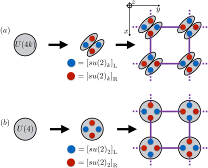
Figure 3: Schematic of two possible generalizations to 3D of the 2D setup depicted in Fig. 1. (a) The generalization presented in Sec. IV.1. In this case, the original wire (gray circle) has a $U(4k)$ symmetry that is broken into two copies of $U(2k)$, on which the conformal embedding (93) is performed. After gapping out the unwanted gapless sectors, the low-energy theory of a single wire is described by two decoupled $su(2)^{\,}_{k}$ CFTs, with each independent copy depicted as residing within a gray oval. The remaining low-energy degrees of freedom are then coupled by interwire current-current interactions (purple bonds), yielding a 3D phase that is equivalent to a stack of decoupled 2D topological phases of the type depicted in Fig. 1. (b) An alternative conformal embedding for $su(2)^{\,}_{2}\oplus su(2)^{\,}_{2}$ into $u(4)^{\,}_{1}$, discussed in Sec. IV.2. In this case the four chiral $su(2)^{\,}_{2}$ modes are depicted as residing within a single gray oval, representing the fact that the two copies of the $su(2)^{\,}_{2}$ CFT are no longer independent, as discussed in Sec. IV.2.

The simplest way to mimic the construction of Sec. III is to generalize the setup depicted in Fig. 1 to a set of wires placed on the sites of a square lattice, as depicted in Fig. 3. Since we will ultimately use current-current bilinears to gap out the array of wires, we need to choose wires that can be broken into a number of chiral channels that matches the coordination number 4 of the square lattice. This can be achieved by choosing wires with an internal symmetry group $U(4k)^{\,}_{\mathrm{L}}\times U(4k)^{\,}_{\mathrm{R}}$, corresponding to wires of the form (1) with $N^{\,}_{\mathrm{c}}=2k$. To obtain four chiral channels, we consider couplings symmetric under the diagonal subgroup $U(2k)\times U(2k)\subset U(4k)$, which effectively breaks each chiral channel $\mathrm{M}=\mathrm{L},\mathrm{R}$ into two identical copies. Then, we can use the identity

$$u(2k)^{\,}_{1}=u(1)\oplus su(2)^{\,}_{k}\oplus su(k)^{\,}_{2}$$ (93)

to define the $\mathrm{M}$-moving chiral currents $\widehat{j}^{\,}_{\mathrm{M},\gamma}$, $\widehat{J}^{a}_{\mathrm{M},\gamma}$, and $\widehat{\mathsf{J}}^{\mathsf{a}}_{\mathrm{M},\gamma}$, where $\gamma=1,2$ labels the two copies. These chiral currents, which are given by Eqs. (4) with the substitution $N^{\,}_{\mathrm{c}}\to k$, correspond to the $u(1)$, $su(2)^{\,}_{k}$, and $su(k)^{\,}_{2}$ sectors, respectively. We then proceed as in Sec. III.1. Namely, we gap out the $u(1)$ and $su(k)^{\,}_{2}$ degrees of freedom by turning on intrawire interactions of the form (8) and (9), respectively, for each $\gamma=1,2$. We then gap out the remaining $su(2)^{\,}_{k}$ channels using bilinear current-current interactions between the wires. This setup is depicted schematically in Fig. 3.

While the above scheme yields a gapped state of matter for the same reasons as the construction presented in Sec. III, this state of matter is not intrinsically 3D. Rather, it can be described as an array of decoupled 2D topological phases of the type constructed in Sec. III. This fact originates from the splitting of the degrees of freedom in the original wire into two groups, $U(4k)\supset U(2k)\times U(2k)$, where the latter two copies of $U(2k)$ are associated with the index $\gamma=1,2$. By splitting up the wire in this way, one imposes the constraint that any local operator in either of the two $su(2)^{\,}_{2}$ CFTs originating from the conformal embedding (93) must be defined exclusively within the $\gamma=1$ or $\gamma=2$ sector. This constraint is represented pictorially in Fig. 3 by the splitting of a gray circle (representing the original wire) into two gray ovals (representing the two channels $\gamma=1,2$). Thus, the array of coupled wires reduces to a set of decoupled planes, each of which is represented by a coupled-wire theory of the type constructed in Sec. III. When the coupled-wire array is defined on a three-torus (i.e., when periodic boundary conditions are imposed in all directions), each plane becomes a two-torus that contributes a factor of $k+1$ to the topological degeneracy, where $k+1$ is the degeneracy of the 2D $su(2)^{\,}_{k}$ topological phase realized by the class of models defined in Sec. III. The total topological degeneracy is then $(k+1)^{p}$, where $p$ is the number of independent planes in the array when periodic boundary conditions are imposed in all directions.

IV.2 Case (2): Reduction to an Abelian phase

One way to avoid reducing the coupled-wire array to a stack of decoupled 2D topological phases is to use a different conformal embedding. To illustrate this, let us take $su(2)^{\,}_{2}$ as our working example. Rather than starting from an array of wires with an internal $U(8)=U(4\times 2)$ symmetry, as outlined in Sec. IV.1, we will use wires with a $U(4)$ internal symmetry and the conformal embedding

$$u(4)^{\,}_{1}=u(1)\oplus su(2)^{\,}_{2}\oplus su(2)^{\,}_{2}.$$ (94)

At first glance, the low-energy theory obtained from the above conformal embedding after gapping the $u(1)$ sector is very similar to the one obtained in Sec. IV.1 by using the conformal embedding (93) on the two copies of the $u(2k)_{1}$ theory with $k=2$. Namely, in both cases the low-energy theory is described by the affine Lie algebra $su(2)^{\,}_{2}\oplus su(2)^{\,}_{2}$. Indeed, in both cases one can also obtain a fully gapped state of matter by adding current-current interactions on the bonds of the square lattice (see Fig. 3).

However, there is a very important physical difference between the theory arising from the conformal embedding (93) and the one arising from the conformal embedding (94). In the former case, the $su(2)^{\,}_{2}\oplus su(2)^{\,}_{2}$ algebra is embedded in a $u(4)_{1}\oplus u(4)_{1}$ algebra, so that each copy of $su(2)^{\,}_{2}$ comes from an independent copy of $u(4)_{1}$. However in the latter case, which is of interest to us here, both copies of $su(2)^{\,}_{2}$ come from the same copy of $u(4)_{1}$. Thus, in the latter case, the two copies of $su(2)^{\,}_{2}$ are not independent but instead nontrivially intertwined. At a technical level, the difference between these two theories is that they have different partition functions. The partition function in the case of the conformal embedding $su(2)^{\,}_{2}\oplus su(2)^{\,}_{2}\subset u(4)_{1}\oplus u(4)_{1}$ is known as the “diagonal” partition function, whereas the partition function in the case of the conformal embedding $su(2)^{\,}_{2}\oplus su(2)^{\,}_{2}\subset u(4)_{1}$ is known as the “off-diagonal” partition function. For explicit expressions for these partition functions, we refer the reader to Sec. 2.2 of Ref. Lah, , which treats the case of two copies of the Ising CFT. The partition functions appearing there can be translated to the $su(2)^{\,}_{2}$ setting simply by making the substitutions $(1,\sigma,\psi)\to(0,\frac{1}{2},1)$, where the symbols on the left hand side label primary fields for the Ising CFT and the symbols on the right-hand side label the primary fields of the $su(2)^{\,}_{2}$ CFT as in Sec. III.3.2. The off-diagonal partition function for the Ising case is associated with the conformal embedding of two Ising CFTs into a $u(1)^{\,}_{4}$ CFT, which is directly analogous to the conformal embedding $su(2)^{\,}_{2}\oplus su(2)^{\,}_{2}\subset u(4)^{\,}_{1}$. [That $u(1)^{\,}_{4}$ is relevant to the Ising case while $u(4)^{\,}_{1}$ is relevant to the $su(2)^{\,}_{2}$ case is a consequence of the fact that the central charge of the Ising $\times$ Ising CFT is $1$, matching the central charge of $u(1)^{\,}_{4}$, while the central charge of the $su(2)^{\,}_{2}\oplus su(2)^{\,}_{2}$ CFT is $3$, matching the central charge of $u(4)^{\,}_{1}/u(1)$.]

As explained in Refs. Lah, and Neupert et al., 2016, the off-diagonal partition function associated with the conformal embedding of two Ising CFTs into a $u(1)^{\,}_{4}$ CFT has an interpretation in terms of anyon condensation Bais and Slingerland (2009) in the Ising $\times$ Ising topological quantum field theory. (This interpretation is a specific instance of the more general correspondence laid out in Ref. Bais and Slingerland, 2009 between anyon condensation and conformal embeddings.) Using this correspondence, one can argue as is done in Refs. Bais and Slingerland, 2009; Neupert et al., 2016; Lah, that the theory described by the off-diagonal partition function is in fact Abelian (as it should be, since the primaries of the $u(1)^{\,}_{4}$ CFT have Abelian fusion rules), even though the underlying Ising $\times$ Ising theory is non-Abelian. This reduction of the non-Abelian theory to an Abelian one arises from constraints imposed by the branching rules of the conformal embedding, which ensure that the two copies of the Ising theory are not independent when embedded within $u(1)^{\,}_{4}$. This argument can be directly extended to the case of the affine Lie algebra $su(2)^{\,}_{2}\oplus su(2)^{\,}_{2}$ considered here if we replace $u(1)^{\,}_{4}$ by $u(4)^{\,}_{1}$. Indeed, we have made extensive use in this paper of the fact that the $su(2)^{\,}_{2}$ CFT is the tensor product of the Ising CFT and the $u(1)^{\,}_{2}$ CFT. We are thus led to the conclusion that the gapped phase obtained from the coupled-wire theory based on the conformal embedding (94) is Abelian, despite the fact that non-Abelian CFTs were used in its construction.

IV.3 Possible workarounds

In order to circumvent the outcomes discussed in Secs. IV.1 and IV.2, one must go beyond the approach used in this paper. We now suggest two possible workarounds that could allow one to construct topological phases that are both (1) intrinsically 3D (i.e., not adiabatically connected to a stack of decoupled 2D topological phases) and (2) support non-Abelian pointlike or stringlike excitations. The approaches we suggest might yield 3D phases described by topological quantum field theories in (3+1)-dimensional spacetime, or could yield phases that, like fracton phases Chamon (2005); Bravyi et al. (2011); Haah (2011); Castelnovo and Chamon (2012); Yoshida (2013); Vijay et al. (2015); Son ; Pre , evade a purely topological field-theoretic description.

IV.3.1 Adding additional intrawire interactions

One approach worth exploring further involves starting from a stack of decoupled 2D topological phases realized using the conformal embedding procedure described in Sec. IV.1, and then adding additional intrawire interactions within the $su(2)^{\,}_{k}\oplus su(2)^{\,}_{k}$ sector. Adding such intrawire interactions would amount to adding couplings between the previously decoupled 2D planes. These couplings should be chosen such that they would not fully gap out the $su(2)^{\,}_{k}\oplus su(2)^{\,}_{k}$ sector of the array of quantum wires if their strength was taken to be much larger than the interwire couplings (if they were not chosen in this way, then the resulting phase would be adiabatically connected to a set of individually gapped, decoupled wires, rendering it topologically trivial). One class of intrawire interactions that might satisfy this condition would be a set of interactions that drive an anyon condensation transition in the case of an isolated bilayer of $su(2)^{\,}_{k}$ topological phases (which can be viewed as a single 2D system). If the 2D condensation transition driven by these interactions yields another gapped non-Abelian topological phase, then there is hope that the 3D phase obtained by coupling more than two layers would also be non-Abelian. This approach would make contact with the coupled-layer construction developed in Ref. Jian and Qi, 2014 for Abelian topological phases (see also Ref. Fuj, ).

In order to move in this direction, it will be important to develop a detailed understanding of how anyon condensation can be implemented in coupled-wire constructions of 2D topological phases by adding appropriate intrawire interactions. This direction is, to our knowledge, as yet unexplored. The possible applications to 3D topological phases mentioned above provide substantial motivation for such a study.

IV.3.2 Moving beyond bilinear current-current interactions

Another aspect of our approach that hampers generalizations to 3D is the fact that we restricted our attention to interwire interactions that are simple bilinears of currents in neighboring wires, as in Eq. (13). Such interactions have the advantage of being both mutually commuting and marginally relevant under RG, and thus they can always be used to open a gap in an array of coupled wires. Furthermore, such bilinear interactions are the most natural ones to use in coupled-wire constructions of 2D topological phases because they can be viewed as dimerizing a 1D cross-section of the 2D system (see Fig. 1). The 3D case is more complicated, however. If we generalize the 1D setup in such a way that a 2D cross-section of the wire array looks like a 2D lattice (see Fig. 3), there are many other kinds of couplings one could imagine adding. For example, one could use couplings defined on plaquettes of the 2D lattice that are products of current-current bilinears. Combining the plethora of (1+1)-dimensional CFTs with the richer set of 2D lattices yields a large space of possible 3D coupled-wire theories that has not yet been explored.

Interactions that cannot be written as bilinears of currents have already been explored in the context of coupled-wire constructions of Abelian topological phases in 3D (see, e.g., Ref. Iadecola et al., 2016). In the non-Abelian case, such interactions suffer from the fact that they are irrelevant under RG as they involve more than two currents. This does not exclude the possibility of using such interactions to open a gap, however, as one can simply treat the system at strong coupling. However, such a treatment necessitates the use of nonperturbative techniques to verify that a gap indeed opens at strong coupling. This was done for the Abelian case in Ref. Iadecola et al., 2016, but the extension to non-Abelian phases is not obvious. We plan to explore the possibility of extending the methods of Ref. Iadecola et al., 2016 to the non-Abelian case in future work.

V Conclusions

In this paper, we studied coupled-wire realizations of $su(2)^{\,}_{k}$ topological phases in two spatial dimensions. These phases inherit their non-Abelian character from the underlying $su(2)^{\,}_{k}$ CFTs that describe the constituent interacting fermionic quantum wires in the decoupled limit. For the special case of $su(2)^{\,}_{2}$, we showed explicitly how to construct a set of nonlocal operators that can be used to label a set of degenerate ground states and to cycle between states in this set, thus demonstrating how the expected threefold degeneracy arises in a coupled-wire construction. This calculation relies on the operator algebra of the underlying CFTs that furnish the low-energy degrees of freedom for the coupled-wire construction, thus making explicit the connection between these CFTs and the emergent topological phase.

There are a number of open directions for the study of coupled-wire constructions that are worth exploring further. One natural question is how to extend the methods developed in this paper for calculating topological degeneracies to the class of 2D topological phases constructed, e.g., in Refs. Teo and Kane, 2014; Huang et al., 2016 whose edge states are described by coset conformal field theories. Another interesting question raised in Sec. IV concerns how to describe anyon condensation transitions Bais and Slingerland (2009) within the coupled-wire framework. As pointed out in Sec. IV.3.1, answering this question could provide a useful path forward for defining interesting non-Abelian coupled-wire models in 3D. A related direction of interest is to study how the gauging of anyonic symmetries in 2D topological order Teo et al. (2015) can be implemented at the level of coupled-wire constructions. This gauging procedure is related to the orbifold construction in CFT Di Francesco et al. (1997); Ginsparg (1988); Dijkgraaf et al. (1989); Moore and Seiberg (1989b), which has been investigated in the context of coupled-wire constructions in Ref. Kane and Stern, 2018. A final direction worth pursuing is to investigate whether more complicated current-current interactions like those suggested in Sec. IV.3.2 could be used to develop new non-Abelian topological phases in 3D.

Appendix A The parafermion current algebra

We are going to review how the affine Lie algebra of level $k=1,2,3,\cdots$ for the compact connected Lie group $SU(2)$ can be represented in terms of parafermions as was done by Zamolodchikov and Fateev in Ref. Zamolodchikov and Fateev, 1985.

A.1 Gaussian algebra

For any $\kappa>0$, define the Euclidean action

$$S\,\raisebox{0.85pt}{.}\raisebox{2.85pt}{.}\!\!=\,\frac{\kappa}{2}\int\mathrm{d}^{2}\bm{x}\,(\bm{\partial}\varphi)^{2}$$ (95)

for the real-valued scalar field $\varphi$ and the positive number $0<\kappa\in\mathbb{R}$. Its two-point function is

$$\langle\varphi(\bm{x})\,\varphi(\bm{y})\rangle=-\frac{1}{4\pi\kappa}\,\ln|\bm{x}-\bm{y}|^{2}$$ (96)

up to an additive dimensionful constant that depends on the boundary condition imposed on the Laplacian. If we trade the complex coordinates $v\in\mathbb{C}$ and $w\in\mathbb{C}$ in two-dimensional Euclidean space for the Cartesian coordinates $\bm{x}\in\mathbb{R}^{2}$ and $\bm{y}\in\mathbb{R}^{2}$, respectively, then

$$|\bm{x}-\bm{y}|^{2}=(v-w)\,(\overline{v}-\overline{w})$$ (97)

and

$$\langle\varphi(\bm{x})\,\varphi(\bm{y})\rangle=-\frac{1}{4\pi\kappa}\,\left[\log(v-w)+\log(\overline{v}-\overline{w})\right],$$ (98a)

$$\langle\partial^{\,}_{v}\varphi(\bm{x})\,\varphi(\bm{y})\rangle=-\frac{1}{4\pi\kappa}\,\frac{1}{(v-w)},$$ (98b)

$$\langle\partial^{\,}_{v}\varphi(\bm{x})\,\partial^{\,}_{w}\varphi(\bm{y})\rangle=-\frac{1}{4\pi\kappa}\,\frac{1}{(v-w)^{2}},$$ (98c)

$$\langle\partial^{\,}_{\overline{v}}\varphi(\bm{x})\,\varphi(\bm{y})\rangle=-\frac{1}{4\pi\kappa}\,\frac{1}{(\overline{v}-\overline{w})},$$ (98d)

$$\langle\partial^{\,}_{\overline{v}}\varphi(\bm{x})\,\partial^{\,}_{\overline{w}}\varphi(\bm{y})\rangle=-\frac{1}{4\pi\kappa}\,\frac{1}{(\overline{v}-\overline{w})^{2}}.$$ (98e)

There follows the chiral Abelian OPEs

$$\partial^{\,}_{v}\varphi(\bm{x})\,\varphi(\bm{y})=-\frac{1}{4\pi\kappa}\,\frac{1}{(v-w)}+\cdots,$$ (99a)

$$\partial^{\,}_{v}\varphi(\bm{x})\,\partial^{\,}_{w}\varphi(\bm{y})=-\frac{1}{4\pi\kappa}\,\frac{1}{(v-w)^{2}}+\cdots,$$ (99b)

$$\partial^{\,}_{\overline{v}}\varphi(\bm{x})\,\varphi(\bm{y})=-\frac{1}{4\pi\kappa}\,\frac{1}{(\overline{v}-\overline{w})}+\cdots,$$ (99c)

$$\partial^{\,}_{\overline{v}}\varphi(\bm{x})\,\partial^{\,}_{\overline{w}}\varphi(\bm{y})=-\frac{1}{4\pi\kappa}\,\frac{1}{(\overline{v}-\overline{w})^{2}}+\cdots,$$ (99d)

$$\partial^{\,}_{v}\varphi(\bm{x})\,\partial^{\,}_{\overline{w}}\varphi(\bm{y})=0.$$ (99e)

The conformal weights of the field $\partial^{\,}_{v}\phi$ are

$$(\Delta^{\,}_{\partial^{\,}_{v}\phi},\overline{\Delta}^{\,}_{\partial^{\,}_{v}\phi})=(1,0).$$ (100)

Another set of chiral Abelian OPEs follows from making the Ansatz

$$\varphi(v,\overline{v})\,=\!\!\raisebox{0.85pt}{.}\raisebox{2.85pt}{.}\,\phi^{\,}_{\mathrm{L}}(v)+\phi^{\,}_{\mathrm{R}}(\overline{v}),$$ (101a)

$$\left\langle\partial^{\,}_{v}\phi^{\,}_{\mathrm{L}}(v)\,\phi^{\,}_{\mathrm{L}}(w)\right\rangle=-\frac{1}{4\pi\,\kappa}\frac{1}{v-w},$$ (101b)

$$\left\langle\partial^{\,}_{v}\phi^{\,}_{\mathrm{R}}(\overline{v})\,\phi^{\,}_{\mathrm{R}}(\overline{w})\right\rangle=-\frac{1}{4\pi\,\kappa}\frac{1}{\overline{v}-\overline{w}},$$ (101c)

$$\left\langle\phi^{\,}_{\mathrm{R}}(v)\,\phi^{\,}_{\mathrm{L}}(\overline{w})\right\rangle=0.$$ (101d)

The holomorphic, $\phi^{\,}_{\mathrm{L}}$, and antiholomorphic, $\phi^{\,}_{\mathrm{R}}$, fields are uniquely defined up to the addition of holomorphic and antiholomorphic functions, respectively. One then deduces from

$$\left\langle e^{+\mathrm{i}a\,\phi^{\,}_{\mathrm{L}}(v)}\,e^{-\mathrm{i}a\,\phi^{\,}_{\mathrm{L}}(w)}\right\rangle=\frac{1}{(v-w)^{\frac{a^{2}}{4\pi\kappa}}},$$ (102a)

$$\left\langle e^{+\mathrm{i}a\,\phi^{\,}_{\mathrm{L}}(v)}\,e^{+\mathrm{i}a\,\phi^{\,}_{\mathrm{L}}(w)}\right\rangle=0,$$ (102b)

$$\left\langle e^{+\mathrm{i}a\,\phi^{\,}_{\mathrm{R}}(\overline{v})}\,e^{-\mathrm{i}a\,\phi^{\,}_{\mathrm{R}}(\overline{w})}\right\rangle=\frac{1}{(\overline{v}-\overline{w})^{\frac{a^{2}}{4\pi\kappa}}},$$ (102c)

$$\left\langle e^{+\mathrm{i}a\,\phi^{\,}_{\mathrm{R}}(\overline{v})}\,e^{+\mathrm{i}a\,\phi^{\,}_{\mathrm{R}}(\overline{w})}\right\rangle=0,$$ (102d)

$$\left\langle e^{\pm\mathrm{i}a\,\phi^{\,}_{\mathrm{L}}(v)}\,e^{\pm\mathrm{i}a\,\phi^{\,}_{\mathrm{R}}(\overline{w})}\right\rangle=0,$$ (102e)

that

$$e^{+\mathrm{i}a\,\phi^{\,}_{\mathrm{L}}(v)}\,e^{-\mathrm{i}a\,\phi^{\,}_{\mathrm{L}}(w)}=\frac{1}{(v-w)^{\frac{a^{2}}{4\pi\kappa}}}$$

$$\hphantom{e^{+\mathrm{i}a\,\phi^{\,}_{\mathrm{L}}(v)}\,e^{-\mathrm{i}a\,\phi^{\,}_{\mathrm{L}}(w)}=}+\frac{\mathrm{i}a}{(v-w)^{\frac{a^{2}}{4\pi\kappa}-1}}\,(\partial^{\,}_{w}\phi^{\,}_{\mathrm{L}})(w)+\cdots,$$ (103a)

$$e^{+\mathrm{i}a\,\phi^{\,}_{\mathrm{R}}(\overline{v})}\,e^{-\mathrm{i}a\,\phi^{\,}_{\mathrm{R}}(\overline{w})}=\frac{1}{(\overline{v}-\overline{w})^{\frac{a^{2}}{4\pi\kappa}}}$$

$$\hphantom{e^{+\mathrm{i}a\,\phi^{\,}_{\mathrm{L}}(v)}\,e^{-\mathrm{i}a\,\phi^{\,}_{\mathrm{L}}(w)}=}+\frac{\mathrm{i}a}{(\overline{z}-\overline{w})^{\frac{a^{2}}{4\pi\kappa}-1}}\,(\partial^{\,}_{\overline{w}}\phi^{\,}_{\mathrm{R}})(\overline{w})+\cdots,$$ (103b)

are the only chiral Abelian OPEs between the vertex fields $e^{\pm\mathrm{i}a\,\phi^{\,}_{\mathrm{L}}(v)}$ and $e^{\pm\mathrm{i}a\,\phi^{\,}_{\mathrm{R}}(\overline{v})}$ that are proportional to the identity operator to leading order.

At last, we shall need the OPEs

$$\partial^{\,}_{v}\phi^{\,}_{\mathrm{L}}(v)\,e^{+\mathrm{i}a\phi^{\,}_{\mathrm{L}}(w)}=-\frac{\mathrm{i}a}{4\pi\kappa}\frac{1}{(v-w)}\,e^{+\mathrm{i}a\phi^{\,}_{\mathrm{L}}(w)}+\cdots,$$ (104a)

$$\partial^{\,}_{\overline{v}}\phi^{\,}_{\mathrm{R}}(\overline{v})\,e^{+\mathrm{i}a\phi^{\,}_{\mathrm{R}}(\overline{w})}=-\frac{\mathrm{i}a}{4\pi\kappa}\frac{1}{(\overline{v}-\overline{w})}\,e^{+\mathrm{i}a\phi^{\,}_{\mathrm{R}}(\overline{w})}+\cdots.$$ (104b)

In the following, we make the choice

$$\kappa=\frac{1}{8\pi}.$$ (105)

With this choice, the conformal weights of the vertex fields $\exp\big{(}\mathrm{i}a\phi^{\,}_{\mathrm{L}}\big{)}$ and $\exp\big{(}\mathrm{i}a\phi^{\,}_{\mathrm{R}}\big{)}$ are

$$(\Delta^{\,}_{a},\overline{\Delta}^{\,}_{a})\equiv(a^{2},0),\qquad(\Delta^{\,}_{\overline{a}},\overline{\Delta}^{\,}_{\overline{a}})\equiv(0,a^{2}),$$ (106)

respectively. Moreover, the proportionality constant on the right-hand side of Eq. (104) is $-2a\mathrm{i}$.

A.2 Parafermion algebra

Let $k=0,1,2,\cdots$ be a positive integer. Define the holomorphic conformal weights

$$\Delta^{\,}_{l}\,\raisebox{0.85pt}{.}\raisebox{2.85pt}{.}\!\!=\,\frac{l(k-l)}{k},\qquad l=0,\cdots,k-1.$$ (107a)

We posit the family of $$k$$ local parafermion fields

$$I,\Psi^{\,}_{1}(v),\cdots,\Psi^{\,}_{k-1}(v),$$ (107b)

where $$I$$ is the identity operator with the conformal weights

$$(\Delta^{\,}_{I},\overline{\Delta}^{\,}_{I})\equiv(\Delta^{\,}_{0},\overline{\Delta}^{\,}_{0})=(0,0).$$ (107c)

For any $$m,n=0,\cdots,k-1$$, we impose the OPEs Zamolodchikov and Fateev (1985)

$$\begin{split}\Psi^{\,}_{m}(v)\,\Psi^{\,}_{n}(v^{\prime})=&\,\frac{C^{\Psi^{\,}_{m+n}}_{\Psi^{\,}_{m}\Psi^{\,}_{n}}\,\Psi^{\,}_{m+n}(v^{\prime})}{(v-v^{\prime})^{\Delta^{\,}_{m}+\Delta^{\,}_{n}-\Delta^{\,}_{m+n}}}+\cdots\end{split}$$ (107d)

with the understanding that $$m+n k$$ is defined modulo , i.e.,

$$\Psi^{\,}_{0}\equiv\Psi^{\,}_{k}\equiv I.$$ (107e)

The complex-valued number $$C^{\Psi^{\,}_{m+n}}_{\Psi^{\,}_{m}\Psi^{\,}_{n}}$$ is called a structure constant. Demanding that the OPEs for the parafermions are associative fixes this structure constant to be the positive roots of Zamolodchikov and Fateev (1985)

$$\begin{split}&\left(C^{\Psi^{\,}_{m+n}}_{\Psi^{\,}_{m}\Psi^{\,}_{n}}\right)^{2}=\\ &\quad\frac{\Gamma(m+n+1)\,\Gamma(k-m+1)\,\Gamma(k-n+1)}{\Gamma(m+1)\,\Gamma(n+1)\,\Gamma(k-m-n+1)\,\Gamma(k+1)},\end{split}$$ (107f)

provided the normalization conditions

$$C^{\Psi^{\,}_{k}}_{\Psi^{\,}_{m}\Psi^{\,}_{k-m}}=1,\qquad m=0,\cdots,k-1$$ (107g)

are imposed.

An important consequence of (107f) is the symmetry

$$C^{\Psi^{\,}_{m+n}}_{\Psi^{\,}_{m}\Psi^{\,}_{n}}=C^{\Psi^{\,}_{m+n}}_{\Psi^{\,}_{n}\Psi^{\,}_{m}}\qquad m,n=0,\cdots,k-1,$$ (108)

under interchanging $m$ and $n$. This is why

$$\Psi^{\,}_{n}(v^{\prime})\,\Psi^{\,}_{m}(v)=(-1)^{\Delta^{\,}_{m+n}-\Delta^{\,}_{m}-\Delta^{\,}_{n}}\,\Psi^{\,}_{m}(v)\,\Psi^{\,}_{n}(v^{\prime}),$$ (109a)

where

$$\Delta^{\,}_{m+n}-\Delta^{\,}_{m}-\Delta^{\,}_{n}=-\frac{2mn}{k}\equiv S^{(k)}_{m,n}.$$ (109b)

We shall call $\pi\,S^{(k)}_{m,n}$ the mutual (self) statistical angle between the parafermion $m$ and the parafermion $n\neq m$ (when $n=m$).

Because the OPE between $\Psi^{\,}_{m}$ and $\Psi^{\,}_{k-m}$ gives the identity operator, we shall use the notation

$$\Psi^{{\dagger}}_{m}\equiv\Psi^{\,}_{k-m}$$ (110a)

for $$m=1,\cdots,k-1 m$$. The self statistical angle of the parafermion is

$$S^{(k)}_{m,m}=-\frac{2m^{2}}{k}.$$ (110b)

The self statistical angle of the parafermion $$k-m$$ is

$$S^{(k)}_{k-m,k-m}=-\frac{2(k-m)^{2}}{k}=S^{(k)}_{m,m}\hbox{ mod }\mathbb{Z}.$$ (110c)

The mutual statistics between parafermion $$m k-m$$ and is

$$S^{(k)}_{m,k-m}=-\frac{2m(k-m)}{k}=-S^{(k)}_{m,m}\hbox{ mod }\mathbb{Z}.$$ (110d)

A.3 Parafermion representation of the $su(2)^{\,}_{k}$ current algebra

The $su(2)^{\,}_{k}$ current algebra is defined by the holomorphic current algebra Di Francesco et al. (1997)

$$J^{a}(v)\,J^{b}(w)=\frac{(k/2)\,\delta^{ab}}{(v-w)^{2}}+\frac{\mathrm{i}\epsilon^{abc}}{(v-w)}\,J^{c}(w)+\cdots$$ (111)

for any $a,b=1,2,3$ together with its antiholomorphic copy. Without loss of generality, we consider only this holomorphic current algebra.

In the basis

$$J^{\pm}\,\raisebox{0.85pt}{.}\raisebox{2.85pt}{.}\!\!=\,J^{1}\pm\mathrm{i}J^{2},\qquad J^{3},$$ (112a)

the holomorphic current algebra (111) reads

$$J^{\pm}(v)\,J^{\pm}(w)=0+\cdots,$$ (112b)

$$J^{+}(v)\,J^{-}(w)=\frac{k}{(v-w)^{2}}+\frac{2}{(v-w)}\,J^{3}(w)+\cdots,$$ (112c)

$$J^{3}(v)\,J^{\pm}(w)=\pm\frac{1}{(v-w)}\,J^{\pm}(w)+\cdots,$$ (112d)

$$J^{3}(v)\,J^{3}(w)=\frac{(k/2)}{(v-w)^{2}}+\cdots.$$ (112e)

We are going to verify that this current algebra can be represented in terms of the Gaussian boson $\phi$ from Appendix A.1 and the pair of parafermions $\Psi^{\,}_{1}\equiv\Psi$ and $\Psi^{\,}_{k-1}\equiv\Psi^{{\dagger}}$ from Appendix A.2.

We make the Ansatz

$$J^{+}(v)=\mathcal{N}\,\Psi^{\,}_{1}(v)\,e^{+\mathrm{i}\sqrt{\frac{1}{k}}\,\phi(v)}$$

$$\hphantom{J^{+}(v)}\equiv\mathcal{N}\,\Psi(v)\,e^{+\mathrm{i}\sqrt{\frac{1}{k}}\,\phi(v)},$$ (113a)

$$J^{-}(v)=\mathcal{N}\,e^{-\mathrm{i}\sqrt{\frac{1}{k}}\,\phi(v)}\Psi^{\,}_{k-1}(v)$$

$$\hphantom{J^{-}(v)}\equiv\mathcal{N}\,e^{-\mathrm{i}\sqrt{\frac{1}{k}}\,\phi(v)}\,\Psi^{{\dagger}}(v),$$ (113b)

$$J^{3}(v)=\mathrm{i}\frac{\sqrt{k}}{2}\,(\partial^{\,}_{v}\phi)(v),$$ (113c)

where we impose on $\partial^{\,}_{v}\phi$ the Gaussian algebra

$$\partial^{\,}_{v}\phi(v)\,\partial^{\,}_{w}\phi(w)=-\frac{2}{(v-w)^{2}}+\cdots,$$ (114a)

while we impose on $$\Psi \Psi^{{\dagger}}$$ and the parafermion algebra

$$\Psi(v)\,\Psi(w)=\frac{C^{I}_{\Psi\Psi}}{(v-w)^{2(k-1)/k}}+\cdots,$$ (114b)

$$\Psi^{{\dagger}}(v)\,\Psi^{{\dagger}}(w)=\frac{C^{I}_{\Psi^{{}^{{\dagger}}}\Psi^{{}^{{\dagger}}}}}{(v-w)^{2(k-1)/k}}+\cdots,$$ (114c)

$$\Psi^{\,}(v)\,\Psi^{{\dagger}}(w)=\frac{1}{(v-w)^{2(k-1)/k}}+\cdots.$$ (114d)

The OPE (112e) follows from the Ansatz (113c) with the OPE (114a). Because of the OPE (104), we have the OPE

$$\partial^{\,}_{v}\phi(v)\,e^{\pm\mathrm{i}\sqrt{\frac{1}{k}}\,\phi(w)}=\mp\mathrm{i}\sqrt{\frac{1}{k}}\,\frac{2}{(v-w)}\,e^{\pm\mathrm{i}\sqrt{\frac{1}{k}}\,\phi(w)}.$$ (115)

The OPE (112d) follows from the Ansatz (113) with the OPE (115). We thus see that the multiplicative factor $\sqrt{1/k}$ entering the argument of the vertex fields $\exp(\pm\mathrm{i}\sqrt{1/k}\,\phi)$ is fixed by the condition that the two currents have the holomorphic conformal weight one. In turn, the normalization factor $\mathcal{N}$ is fixed by the following considerations. Because of the OPEs (107) and (103), we have the OPE

$$J^{+}(v)\,J^{-}(w)= \,\mathcal{N}^{2}\,\Psi^{\,}_{1}(v)\,\Psi^{\,}_{k-1}(w)\,e^{+\mathrm{i}\sqrt{\frac{1}{k}}\,\phi(v)}\,e^{-\mathrm{i}\sqrt{\frac{1}{k}}\,\phi(w)}$$

$$= \,\left(\frac{\mathcal{N}^{2}}{(v-w)^{1-\frac{1}{k}+1-\frac{1}{k}}}+\cdots\right)\frac{1}{(v-w)^{\frac{2}{k}}}\left(1+\mathrm{i}\sqrt{\frac{1}{k}}\,(v-w)(\partial^{\,}_{w}\phi)(w)+\cdots\right)$$

$$= \,\frac{\mathcal{N}^{2}}{(v-w)^{2}}+\frac{(2\mathcal{N}^{2}/k)}{(v-w)}\,J^{3}(w)+\cdots.$$ (116)

The leading singularity on the right-hand side of this OPE agrees with the one on the right-hand side of Eq. (112c) if

$$\mathcal{N}^{2}=k.$$ (117)

Finally, the vanishing OPE (112b) follows from the fact that the OPE between any two vertex fields such that the $\mathbb{C}$-valued prefactors to the fields $\phi(v)$ and $\phi(w)$ in the arguments of the vertex fields are not of opposite sign, vanishes to leading order.

We close Appendix A.3 by observing that the Ansatz (113) is not unique. Indeed, the transformation

$$\Psi(v)\mapsto\Psi(v)\,e^{+\mathrm{i}\alpha},$$ (118a)

$$\Psi^{{\dagger}}(v)\mapsto\Psi^{{\dagger}}(v)\,e^{-\mathrm{i}\alpha},$$ (118b)

$$\phi(v)\mapsto\phi(v)-\sqrt{k}\,\alpha,$$ (118c)

leaves the $su(2)^{\,}_{k}$ currents (112a) invariant for any choice of the number $\alpha$. The number $\alpha$ is defined modulo $2\pi$ and takes $k$ inequivalent values $2\pi n/k$, $n=0,\cdots,k-1$.

Appendix B Commutation of string operators and the Hamiltonian; “Analytic” proof of state exclusion

B.1 Introduction

We are given the Hamiltonian

$$\widehat{H}^{\,}_{\mathrm{bs}}\,\raisebox{0.85pt}{.}\raisebox{2.85pt}{.}\!\!=\,\int\limits_{0}^{L^{\,}_{z}}\mathrm{d}z\,\widehat{\mathcal{H}}^{\,}_{\mathrm{bs}}$$ (119)

and we are told that it commutes with two nonlocal operators $\widehat{\Gamma}^{(1)}_{1}$ and $\widehat{\Gamma}^{(1)}_{2}$. Moreover, we are told that $\widehat{\Gamma}^{(1)}_{1}$ and $\widehat{\Gamma}^{(1)}_{2}$ commute pairwise. Hence, we can label any eigenstate of the Hamiltonian $\widehat{H}^{\,}_{\mathrm{bs}}$ by the simultaneous eigenvalues $\omega^{(1)}_{1}$ and $\omega^{(1)}_{2}$ of the operators $\widehat{\Gamma}^{(1)}_{1}$ and $\widehat{\Gamma}^{(1)}_{2}$. In particular, we can label the basis for the ground-state manifold by

$$\{|\omega^{(1)}_{1},\omega^{(1)}_{2},\cdots\rangle\}$$ (120)

where the $\cdots$ allow for additional sources of degeneracies. We shall demand that this basis is orthonormal.

In order to establish the set to which the eigenvalues $\omega^{(1)}_{1}$ and $\omega^{(1)}_{2}$ belong, we note that we are given two nonlocal operators

$$\widehat{\Gamma}^{(\frac{1}{2})}_{1}(t,z) \,\raisebox{0.85pt}{.}\raisebox{2.85pt}{.}\!\!=\,\prod_{y=0}^{L^{\,}_{y}}\widehat{\sigma}^{\,}_{\mathrm{L},y}(t,z)\,\widehat{\sigma}^{\,}_{\mathrm{R},y}(t,z),$$ (121a)

and

$$\begin{split}\widehat{\Gamma}^{(\frac{1}{2})}_{\mathrm{R},2,y}(t,\epsilon)&\,\raisebox{0.85pt}{.}\raisebox{2.85pt}{.}\!\!=\,\,\exp\Bigg{(}-\frac{\mathrm{i}}{2\sqrt{2}}\int\limits^{L^{\,}_{z}}_{0}\mathrm{d}z\,\partial^{\,}_{z}\widehat{\phi}^{\,}_{\mathrm{R},y}(t,z)\Bigg{)}\\ &\qquad\times\,\widehat{\mathcal{P}}^{\,}_{\mathbbm{1}}\,\widehat{\sigma}^{\,}_{\mathrm{R},y}(t,0)\,\widehat{\sigma}^{\,}_{\mathrm{R},y}(t,\epsilon)\,\widehat{\mathcal{P}}^{\,}_{\mathbbm{1}}\end{split}$$ (121b)

$$\equiv\,\widehat{\mathcal{U}}\,\times\,\widehat{\mathcal{P}}^{\,}_{\mathbbm{1}}\,\widehat{\sigma}^{\,}_{\mathrm{R},y}(t,0)\,\widehat{\sigma}^{\,}_{\mathrm{R},y}(t,\epsilon)\,\widehat{\mathcal{P}}^{\,}_{\mathbbm{1}}.$$ (121c)

The operator $\widehat{\Gamma}^{(\frac{1}{2})}_{1}$ is a discrete product of a countable number of operators acting along a closed $y$-cycle of the two-torus. It requires no regularization for its definition. It anticommutes with $\widehat{\Gamma}^{(1)}_{2}$, and commutes with $\widehat{\Gamma}^{(1)}_{1}$ and with the Hamiltonian (119). In contrast, the operator $\widehat{\Gamma}^{(\frac{1}{2})}_{\mathrm{R},2,y}(t,\epsilon)$ is a nonlocal operator defined within one chiral channel of the wire $y$. It acts along an open string (along the $z$-cycle coinciding with wire $y$) that fails to close by the infinitesimal amount $\epsilon>0$. It anticommutes with $\widehat{\Gamma}^{(1)}_{1}$ in the limit $\epsilon\to 0$.

If both $\widehat{\Gamma}^{(\frac{1}{2})}_{1}(t,z)$ and $\lim_{\epsilon\to 0}\widehat{\Gamma}^{(\frac{1}{2})}_{\mathrm{R},2,y}(t,\epsilon)$ were to commute with the Hamiltonian, then so would their product. The ground-state manifold would then be four-dimensional, with the orthogonal basis

$$|\Omega,\cdots\rangle\,\raisebox{0.85pt}{.}\raisebox{2.85pt}{.}\!\!=\,|\omega^{(1)}_{1},\omega^{(1)}_{2},\cdots\rangle,$$ (122a)

$$\widehat{\Gamma}^{(\frac{1}{2})}_{1}(t,z)\,|\Omega,\cdots\rangle\equiv\mathcal{N}^{\,}_{1}\,|\omega^{(1)}_{1},-\omega^{(1)}_{2},\cdots\rangle,$$ (122b)

$$\lim_{\epsilon\to 0}\widehat{\Gamma}^{(\frac{1}{2})}_{\mathrm{R},2,y}(t,\epsilon)\,|\Omega,\cdots\rangle\equiv\mathcal{N}^{\,}_{2}\,|-\omega^{(1)}_{1},\omega^{(1)}_{2},\cdots\rangle,$$ (122c)

$$\begin{split}&\widehat{\Gamma}^{(\frac{1}{2})}_{1}(t,z)\,\left[\lim_{\epsilon\to 0}\widehat{\Gamma}^{(\frac{1}{2})}_{\mathrm{R},2,y}(t,\epsilon)\,|\Omega,\cdots\rangle\right]\\ &\qquad\qquad\qquad\equiv\mathcal{N}^{\,}_{12}\,|-\omega^{(1)}_{1},-\omega^{(1)}_{2},\cdots\rangle,\end{split}$$ (122d)

$$\cdots.$$ (122e)

We demand that the states on the left-hand side can be normalized. This can only be achieved if the normalizations $\mathcal{N}^{\,}_{1}$, $\mathcal{N}^{\,}_{2}$, and $\mathcal{N}^{\,}_{12}$ are neither zero nor infinity, for the basis (120) is orthonormal by assumption.

However, the logical possibility that one or more of these normalizations are zero or infinity cannot be excluded. In this appendix, we will assume $\mathcal{N}^{\,}_{1}$ and $\mathcal{N}^{\,}_{2}$ to be nonvanishing and finite. This assumption amounts to choosing the “highest-weight state” (122a) appropriately. The quantity $\mathcal{N}^{\,}_{12}$ could be determined by direct calculation, provided that the explicit form of the state $\ket{\Omega,\cdots}$ is known. Since we do not have this knowledge, we leave its value unspecified for the moment.

Given that we do not know the value of $\mathcal{N}^{\,}_{12}$, we proceed by an alternate route. This line of reasoning makes use of the fact that it is not correct to think of the operator $\lim_{\epsilon\to 0}\widehat{\Gamma}^{(\frac{1}{2})}_{\mathrm{R},2,y}(t,\epsilon)$ as commuting with the Hamiltonian (119). It is a nonlocal operator that changes the topological sector of the state on which it acts, and can potentially exhibit different limiting behavior as a function of $\epsilon$ when acting on states belonging to different topological sectors. Thus, the limit $\epsilon\to 0$ must be treated carefully when multiplying the operators $\widehat{\Gamma}^{(\frac{1}{2})}_{\mathrm{R},2,y}(t,\epsilon)$ and $\widehat{\Gamma}^{(\frac{1}{2})}_{1}$. Indeed, instead of the set of states (122), we can also consider the following set of states,

$$|\Omega,\cdots\rangle\,\raisebox{0.85pt}{.}\raisebox{2.85pt}{.}\!\!=\,|\omega^{(1)}_{1},\omega^{(1)}_{2},\cdots\rangle,$$ (123a)

$$\ket{\widehat{\Gamma}^{(\frac{1}{2})}_{1},\cdots}\,\raisebox{0.85pt}{.}\raisebox{2.85pt}{.}\!\!=\,\widehat{\Gamma}^{(\frac{1}{2})}_{1}(t,z)\,|\Omega,\cdots\rangle,$$ (123b)

$$\ket{\widehat{\Gamma}^{(\frac{1}{2})}_{2},\cdots}\,\raisebox{0.85pt}{.}\raisebox{2.85pt}{.}\!\!=\,\lim_{\epsilon\to 0}\widehat{\Gamma}^{(\frac{1}{2})}_{\mathrm{R},2,y}(t,\epsilon)\ket{\Omega,\cdots},$$ (123c)

$$\ket{\widehat{\Gamma}^{(\frac{1}{2})}_{1}\widehat{\Gamma}^{(\frac{1}{2})}_{2},\cdots}\,\raisebox{0.85pt}{.}\raisebox{2.85pt}{.}\!\!=\,\lim_{\epsilon\to 0}\left[\widehat{\Gamma}^{(\frac{1}{2})}_{1}(t,z)\,\widehat{\Gamma}^{(\frac{1}{2})}_{\mathrm{R},2,y}(t,\epsilon)\ket{\Omega,\cdots}\right].$$ (123d)

The only difference between the states (123) and the states (122) is that the limit $\epsilon\to 0$ is taken after forming the product $\widehat{\Gamma}^{(\frac{1}{2})}_{1}\,\widehat{\Gamma}^{(\frac{1}{2})}_{\mathrm{R},2,y}(t,\epsilon)$ in Eq. (123d). We adopt the point of view that the dimension of the ground-state manifold of the Hamiltonian (119) cannot depend on the choice of when [i.e., before or after forming the product $\widehat{\Gamma}^{(\frac{1}{2})}_{1}\,\widehat{\Gamma}^{(\frac{1}{2})}_{\mathrm{R},2,y}(t,\epsilon)$] the limit $\epsilon\to 0$ is taken. Hence, the number of ground states present in Eqs. (122) and (123) must agree with one another. For this reason, we ask how many of the states (123) are indeed ground states of the interaction (119). This allows us to scrutinize the limiting behavior of operator products without losing important information related to the nonlocality of its constituent operators. We will show that the state (123d) cannot be in the ground-state manifold of the interaction (119). Logical consistency then demands that $\mathcal{N}^{\,}_{12}=0$ or $\infty$ in Eqs. (122), as these are the only two possibilities that would exclude the state (122d) from the ground-state manifold.

The operator $\widehat{\Gamma}^{(\frac{1}{2})}_{\mathrm{R},2,y}(t,\epsilon)$ does not commute with the interaction $\widehat{H}^{\,}_{\mathrm{bs}}$ defined by Eq. (119). The purpose of this appendix is to determine whether the states (123c) and (123d), which involve taking the limit $\epsilon\to 0$, indeed belong to the ground-state manifold of the interaction (119) once this limit is taken. More precisely, we define

$$\left[\widehat{H}^{\,}_{\mathrm{bs}},\widehat{\Gamma}^{(\frac{1}{2})}_{\mathrm{R},2,y}(t,\epsilon)\right]\,=\!\!\raisebox{0.85pt}{.}\raisebox{2.85pt}{.}\,\widehat{\mathcal{D}}^{\,}_{\mathrm{R},2,y}(t,\epsilon),$$ (124a)

where the operator $$\widehat{\mathcal{D}}^{\,}_{\mathrm{R},2,y}(t,\epsilon)$$ is nonlocal, as we shall see below, and nonvanishing in general. We further define

$$\begin{split}\left[\widehat{H}^{\,}_{\mathrm{bs}},\widehat{\Gamma}^{(\frac{1}{2})}_{1}(t,z)\,\widehat{\Gamma}^{(\frac{1}{2})}_{\mathrm{R},2,y}(t,\epsilon)\right]&=\widehat{\Gamma}^{(\frac{1}{2})}_{1}(t,z)\,\widehat{\mathcal{D}}^{\,}_{\mathrm{R},2,y}(t,\epsilon)\\ &\,=\!\!\raisebox{0.85pt}{.}\raisebox{2.85pt}{.}\,\widehat{\mathcal{D}}^{\,}_{1\mathrm{R},2,y}(z,\epsilon).\end{split}$$ (124b)

We are going to show that

$$\lim_{\epsilon\to 0}\widehat{\mathcal{D}}^{\,}_{\mathrm{R},2,y}(t,\epsilon)\ket{\Omega,\cdots} =0.$$ (125a)

Equation (125a) is equivalent to the statement

$$\lim_{\epsilon\to 0}\left[\widehat{H}^{\,}_{\mathrm{bs}},\widehat{\Gamma}^{(\frac{1}{2})}_{\mathrm{R},2,y}(t,\epsilon)\right]\ket{\Omega,\cdots}=(\widehat{H}^{\,}_{\mathrm{bs}}-E^{\,}_{\Omega})\,\ket{\widehat{\Gamma}^{(\frac{1}{2})}_{2},\cdots}=0,$$ (125b)

where $E^{\,}_{\Omega}$ is the energy eigenvalue of the state $\ket{\Omega,\cdots}$. From this it immediately follows that the state $\ket{\widehat{\Gamma}^{(\frac{1}{2})}_{2},\cdots}$ indeed belongs to the ground-state manifold of the interaction (119).

We are also going to show that the state

$$\lim_{\epsilon\to 0}\widehat{\mathcal{D}}^{\,}_{1\mathrm{R},2,y}(z,\epsilon)\ket{\Omega,\cdots}$$ (126a)

has infinite norm as $$z\to 0$$. Equation (126a) is equivalent to the statement that

$$\begin{split}&\lim_{z\to 0}\lim_{\epsilon\to 0}\left[\widehat{H}^{\,}_{\mathrm{bs}},\widehat{\Gamma}^{(\frac{1}{2})}_{1}(t,z)\,\widehat{\Gamma}^{(\frac{1}{2})}_{\mathrm{R},2,y}(t,\epsilon)\right]\ket{\Omega,\cdots}\\ &\qquad\qquad=\lim_{z\to 0}\left(\widehat{H}^{\,}_{\mathrm{bs}}\,-E^{\,}_{\Omega}\right)\ket{\widehat{\Gamma}^{(\frac{1}{2})}_{1}\widehat{\Gamma}^{(\frac{1}{2})}_{2},\cdots}\end{split}$$ (126b)

is a state with infinite norm. That this divergence occurs as $z\to 0$ is especially problematic. In order for the product $\widehat{\Gamma}^{(\frac{1}{2})}_{1}(t,z)\widehat{\Gamma}^{(\frac{1}{2})}_{\mathrm{R},2,y}(t,\epsilon)$ of string operators to yield a topologically-degenerate ground state when acting on the state $\ket{\Omega,\cdots}$, the resulting state cannot depend on the quantities $z$ and $\epsilon$ in an observable way as $z\to 0$ and $\epsilon\to 0$. If this were the case, then the states $\ket{\Omega,\cdots}$ and $\ket{\widehat{\Gamma}^{(\frac{1}{2})}_{1}\widehat{\Gamma}^{(\frac{1}{2})}_{2},\cdots}$ could be distinguished by simply evaluating the string operator $\widehat{\Gamma}^{(\frac{1}{2})}_{1}(t,z)$ near the point $z=0$. Hence, proving that the state defined in Eq. (126a) is not normalizable will allow us to conclude that the state $\ket{\widehat{\Gamma}^{(\frac{1}{2})}_{1}\,\widehat{\Gamma}^{(\frac{1}{2})}_{2},\cdots}$ does not belong to the ground-state manifold of the interaction (119).

We are left with the conclusion of the paper, namely that the ground-state manifold of the interaction (119) includes the states (123a)–(123c), and excludes the state (123d). From now on, we ignore the $\cdots$ representing additional degeneracies for the ground-state manifold.

B.2 Calculation

We first prove Eq. (125a). We begin by calculating $\widehat{\mathcal{D}}^{\,}_{\mathrm{R},2,y}(t,\epsilon)$. For finite $\epsilon>0$, we have

$$\widehat{\mathcal{H}}^{\,}_{\mathrm{bs}}\,\widehat{\Gamma}^{(\frac{1}{2})}_{\mathrm{R},2,y}(t,\epsilon) =\widehat{\Gamma}^{(\frac{1}{2})}_{\mathrm{R},2,y}(t,\epsilon)\,\widehat{\mathcal{H}}^{\,}_{\mathrm{bs}}\,\times\begin{cases}+1,&z>\epsilon,\\ +\mathrm{i},&z=\epsilon,\\ -1,&z<\epsilon.\end{cases}$$ (127)

We now use the definition (124a), along with the identity

$$\widehat{A}\,\widehat{B} =\widehat{B}\,\widehat{A}\,f(z,\epsilon)\iff\left[\widehat{A},\widehat{B}\right]=\widehat{B}\,\widehat{A}\,\left[f(z,\epsilon)-1\right],$$ (128)

which gives

$$\widehat{\mathcal{D}}^{\,}_{\mathrm{R},2,y}(t,\epsilon)= \,-4\mathrm{i}\int\limits^{\epsilon}_{0}\!\mathrm{d}z\,\sin\left(\frac{1}{\sqrt{2}}\left(\widehat{\phi}^{\,}_{\mathrm{R},y}(t,z)-\widehat{\phi}^{\,}_{\mathrm{L},y+1}(t,z)\right)\right)\,\widehat{\mathcal{U}}\,\widehat{\psi}^{\,}_{\mathrm{L},y+1}(t,z)\,\widehat{\psi}^{\,}_{\mathrm{R},y}(t,z)\,\widehat{\mathcal{P}}^{\,}_{\mathbbm{1}}\,\widehat{\sigma}^{\,}_{\mathrm{R},y}(t,0)\,\widehat{\sigma}^{\,}_{\mathrm{R},y}(t,\epsilon)\,\widehat{\mathcal{P}}^{\,}_{\mathbbm{1}},$$ (129)

up to a contribution from the set of measure zero where $z=\epsilon$, which we will ignore.

To prove Eq. (125a), we compute the leading contribution to $\widehat{\mathcal{D}}^{\,}_{2}(t,\epsilon)$ as $\epsilon\to 0$. For $\epsilon$ infinitesimal, we may replace the integral in Eq. (129) by the value of the integrand at the midpoint of the integration domain,

$$\begin{split}\widehat{\mathcal{D}}^{\,}_{\mathrm{R},2,y}(t,\epsilon)\approx-4\mathrm{i}\,\epsilon\,\sin\left(\frac{1}{\sqrt{2}}\left[\widehat{\phi}^{\,}_{\mathrm{R},y}\left(\frac{\epsilon}{2}\right)-\widehat{\phi}^{\,}_{\mathrm{L},y+1}\left(\frac{\epsilon}{2}\right)\right]\right)\,\widehat{\mathcal{U}}\,\widehat{\psi}^{\,}_{\mathrm{L},y+1}\left(\frac{\epsilon}{2}\right)\,\widehat{\psi}^{\,}_{\mathrm{R},y}\left(\frac{\epsilon}{2}\right)\,\widehat{\mathcal{P}}^{\,}_{\mathbbm{1}}\,\widehat{\sigma}^{\,}_{\mathrm{R},y}(t,0)\,\widehat{\sigma}^{\,}_{\mathrm{R},y}(t,\epsilon)\,\widehat{\mathcal{P}}^{\,}_{\mathbbm{1}}.\end{split}$$ (130)

We now perform the (equal-time) OPE

$$\sin\left(\frac{1}{\sqrt{2}}\left[\widehat{\phi}^{\,}_{\mathrm{R},y}\left(\frac{\epsilon}{2}\right)-\widehat{\phi}^{\,}_{\mathrm{L},y+1}\left(\frac{\epsilon}{2}\right)\right]\right)\,\widehat{\mathcal{U}}= \,\sin\left(\frac{1}{\sqrt{2}}\left[\widehat{\phi}^{\,}_{\mathrm{R},y}\left(\frac{\epsilon}{2}\right)-\widehat{\phi}^{\,}_{\mathrm{L},y+1}\left(\frac{\epsilon}{2}\right)\right]\right)\,\exp\Bigg{(}\!-\!\frac{\mathrm{i}}{2\sqrt{2}}\int\limits^{L^{\,}_{z}}_{0}\mathrm{d}z\,\partial^{\,}_{z}\,\widehat{\phi}^{\,}_{\mathrm{R},y}(t,z)\Bigg{)}.$$ (131)

Inserting the OPEs

$$\lim_{\epsilon\to 0}e^{+\frac{\mathrm{i}}{\sqrt{2}}\widehat{\phi}^{\,}_{\mathrm{R},y}\left(\frac{\epsilon}{2}\right)}e^{-\frac{\mathrm{i}}{2\sqrt{2}}\widehat{\phi}^{\,}_{\mathrm{R},y}(L^{\,}_{z})}\sim\frac{1}{\epsilon^{1/2}}\,e^{+\frac{\mathrm{i}}{2\sqrt{2}}\widehat{\phi}^{\,}_{\mathrm{R},y}(\frac{\epsilon}{2})},$$ (132a)

$$\lim_{\epsilon\to 0}e^{-\frac{\mathrm{i}}{\sqrt{2}}\widehat{\phi}^{\,}_{\mathrm{R},y}(\frac{\epsilon}{2})}e^{+\frac{\mathrm{i}}{2\sqrt{2}}\widehat{\phi}^{\,}_{\mathrm{R},y}\left(0\right)}\sim\frac{1}{\epsilon^{1/2}}\,e^{-\frac{\mathrm{i}}{2\sqrt{2}}\widehat{\phi}^{\,}_{\mathrm{R},y}(\frac{\epsilon}{2})},$$ (132b)

$$\lim_{\epsilon\to 0}e^{+\frac{\mathrm{i}}{2\sqrt{2}}\widehat{\phi}^{\,}_{\mathrm{R},y}(\frac{\epsilon}{2})}e^{+\frac{\mathrm{i}}{2\sqrt{2}}\widehat{\phi}^{\,}_{\mathrm{R},y}\left(0\right)}\sim\epsilon^{1/4}\,e^{+\frac{\mathrm{i}}{\sqrt{2}}\widehat{\phi}^{\,}_{\mathrm{R},y}(\frac{\epsilon}{2})},$$ (132c)

$$\lim_{\epsilon\to 0}e^{-\frac{\mathrm{i}}{2\sqrt{2}}\widehat{\phi}^{\,}_{\mathrm{R},y}(L^{\,}_{z})}e^{-\frac{\mathrm{i}}{2\sqrt{2}}\widehat{\phi}^{\,}_{\mathrm{R},y}\left(\frac{\epsilon}{2}\right)}\sim\epsilon^{1/4}\,e^{-\frac{\mathrm{i}}{\sqrt{2}}\widehat{\phi}^{\,}_{\mathrm{R},y}(\frac{\epsilon}{2})},$$ (132d)

where “$\sim$” denotes equality up to constant factors and nonsingular terms, and using the fact that $L^{\,}_{z}\sim 0$ by periodic boundary conditions, we find

$$\sin\left(\frac{1}{\sqrt{2}}\left[\widehat{\phi}^{\,}_{\mathrm{R},y}\left(\frac{\epsilon}{2}\right)-\widehat{\phi}^{\,}_{\mathrm{L},y+1}\left(\frac{\epsilon}{2}\right)\right]\right)\,\widehat{\mathcal{U}}\sim \,\frac{1}{\epsilon^{1/4}}\,\sin\left(\frac{1}{\sqrt{2}}\left[\widehat{\phi}^{\,}_{\mathrm{R},y}\left(\frac{\epsilon}{2}\right)-\widehat{\phi}^{\,}_{\mathrm{L},y+1}\left(\frac{\epsilon}{2}\right)\right]\right).$$ (133)

Next, we perform the OPE

$$\widehat{\mathcal{P}}^{\,}_{\mathbbm{1}}\,\widehat{\sigma}^{\,}_{\mathrm{R},y}(t,0)\,\widehat{\sigma}^{\,}_{\mathrm{R},y}(t,\epsilon)\,\widehat{\mathcal{P}}^{\,}_{\mathbbm{1}} \sim\frac{1}{\epsilon^{1/8}}.$$ (134)

Inserting this pair of OPEs into Eq. (130), we find

$$\begin{split}\lim_{\epsilon\to 0}\widehat{\mathcal{D}}^{\,}_{\mathrm{R},2,y}(t,\epsilon)\ket{\Omega}&\sim\lim_{\epsilon\to 0}\epsilon^{5/8}\,\sin\left(\frac{1}{\sqrt{2}}\left[\widehat{\phi}^{\,}_{\mathrm{R},y}\left(\frac{\epsilon}{2}\right)-\widehat{\phi}^{\,}_{\mathrm{L},y+1}\left(\frac{\epsilon}{2}\right)\right]\right)\,\widehat{\psi}^{\,}_{\mathrm{L},y+1}\left(\frac{\epsilon}{2}\right)\,\widehat{\psi}^{\,}_{\mathrm{R},y}\left(\frac{\epsilon}{2}\right)\ket{\Omega}=0.\end{split}$$ (135)

The form of the operator appearing on the RHS above is not important. All that matters is that its expectation value in the state $\ket{\Omega}$ is not singular in the limit $\epsilon\to 0$. Also of crucial importance is the factor $\epsilon^{5/8}$ that sends $\lim_{\epsilon\to 0}\widehat{\mathcal{D}}^{\,}_{\mathrm{R},2,y}(t,\epsilon)\ket{\Omega}\to 0$ as $\epsilon\to 0$. Hence, we may conclude that the state $\ket{\widehat{\Gamma}^{(\frac{1}{2})}_{2}}$, defined in Eq. (123c), is a ground state.

We now turn to the state $\ket{\widehat{\Gamma}^{(\frac{1}{2})}_{1}\,\widehat{\Gamma}^{(\frac{1}{2})}_{2}}$, defined in Eq. (123d), and ask if it, too, is a ground state. We will see that it cannot be a ground state by proving that the state defined in Eq. (126a) has infinite norm as $z\to 0$ and $\epsilon\to 0$. We proceed by setting $z=z^{\,}_{0}=0$ from the outset. Using Eq. (130),

$$\begin{split}\widehat{\Gamma}^{(\frac{1}{2})}_{1}(t,0)\,\widehat{\mathcal{D}}^{\,}_{\mathrm{R},2,y}(t,\epsilon)\approx&\,-4\mathrm{i}\,\epsilon\,\Bigg{(}\prod_{y^{\prime}}\widehat{\sigma}^{\,}_{\mathrm{L},y^{\prime}}(t,0)\,\widehat{\sigma}^{\,}_{\mathrm{R},y^{\prime}}(t,0)\Bigg{)}\,\sin\left(\frac{1}{\sqrt{2}}\left[\widehat{\phi}^{\,}_{\mathrm{R},y}\left(\frac{\epsilon}{2}\right)-\widehat{\phi}^{\,}_{\mathrm{L},y+1}\left(\frac{\epsilon}{2}\right)\right]\right)\,\widehat{\mathcal{U}}\,\\ &\,\times\widehat{\psi}^{\,}_{\mathrm{L},y+1}\left(\frac{\epsilon}{2}\right)\,\widehat{\psi}^{\,}_{\mathrm{R},y}\left(\frac{\epsilon}{2}\right)\,\widehat{\mathcal{P}}^{\,}_{\mathbbm{1}}\,\widehat{\sigma}^{\,}_{\mathrm{R},y}(t,0)\,\widehat{\sigma}^{\,}_{\mathrm{R},y}(t,\epsilon)\,\widehat{\mathcal{P}}^{\,}_{\mathbbm{1}}.\end{split}$$ (136)

Using the OPEs (131) in conjunction with the OPEs

$$\widehat{\sigma}^{\,}_{\mathrm{R},y}(t,0)\,\widehat{\psi}^{\,}_{\mathrm{R},y}\left(\frac{\epsilon}{2}\right)\sim\frac{1}{\epsilon^{1/2}}\,\widehat{\sigma}^{\,}_{\mathrm{R},y}(t,0),$$ (137a)

$$\widehat{\sigma}^{\,}_{\mathrm{L},y+1}(t,0)\,\widehat{\psi}^{\,}_{\mathrm{L},y+1}\left(\frac{\epsilon}{2}\right)\sim\frac{1}{\epsilon^{1/2}}\,\widehat{\sigma}^{\,}_{\mathrm{L},y+1}(t,0),$$ (137b)

we find

$$\widehat{\Gamma}^{(\frac{1}{2})}_{1}(t,0)\,\widehat{\mathcal{D}}^{\,}_{\mathrm{R},2,y}(t,\epsilon)\sim\frac{1}{\epsilon^{3/8}}\sin\left(\frac{1}{\sqrt{2}}\left[\widehat{\phi}^{\,}_{\mathrm{R},y}\left(\frac{\epsilon}{2}\right)-\widehat{\phi}^{\,}_{\mathrm{L},y+1}\left(\frac{\epsilon}{2}\right)\right]\right)\,\widehat{\Gamma}^{(\frac{1}{2})}_{1}(t,0).$$

In contrast to the RHS of Eq. (135), we now have the product between a local operator and a nonlocal operator on the RHS. Furthermore, the real-valued prefactor is a function of $\epsilon$ that diverges as $\epsilon\to 0$. We conclude that

$$\lim_{\epsilon\to 0}\widehat{\mathcal{D}}^{\,}_{1\mathrm{R},2,y}(0,\epsilon)\ket{\Omega} =\widehat{\Gamma}^{(\frac{1}{2})}_{1}(t,0)\,\widehat{\mathcal{D}}^{\,}_{\mathrm{R},2,y}(t,\epsilon)\ket{\Omega}\sim\frac{1}{\epsilon^{3/8}}\sin\left(\frac{1}{\sqrt{2}}\left[\widehat{\phi}^{\,}_{\mathrm{R},y}\left(\frac{\epsilon}{2}\right)-\widehat{\phi}^{\,}_{\mathrm{L},y+1}\left(\frac{\epsilon}{2}\right)\right]\right)\ket{\widehat{\Gamma}^{(\frac{1}{2})}_{1}}$$ (138)

is a state with infinite norm, as advertised, provided that the operator $\sin\Big{(}\frac{1}{\sqrt{2}}[\widehat{\phi}^{\,}_{\mathrm{R},y}(\epsilon/2)-\widehat{\phi}^{\,}_{\mathrm{L},y+1}(\epsilon/2)]\Big{)}$ does not annihilate the state $\ket{\widehat{\Gamma}^{(\frac{1}{2})}_{1}}$. (Determining whether or not this is the case again requires an explicit expression for the state $\ket{\Omega}$, which we do not have at our disposal.) In that case, we conclude that the state $\ket{\widehat{\Gamma}^{(\frac{1}{2})}_{1}\,\widehat{\Gamma}^{(\frac{1}{2})}_{2}}$ cannot be a ground state of the interaction $\widehat{H}^{\,}_{\mathrm{bs}}$ defined by Eq. (119).

Appendix C Diagrammatics for operator algebra in the Ising CFT

The discussion surrounding Eqs. (36) in the main text concerns how to infer the exchange algebra of two chiral primary operators in the Ising CFT from their operator product expansion. This exchange algebra is simple to determine in cases where the two primary operators have a unique fusion product, as in the case of the $\sigma$ and $\psi$ operators in Eqs. (36). However, when the two primary operators do not have a unique fusion product, as occurs in the case of two $\sigma$ operators [see the OPEs in Eqs. (37)], the exchange algebra depends on the fusion channel in which the product of the pair of operators is evaluated [see the exchange algebra in Eqs. (38)]. This poses a challenge for calculations. It is necessary to keep track of both fusion and braiding in a way that respects consistency conditions between the two. This challenge is the essence of the difference between Abelian and non-Abelian excitations in quantum field theory.

To this end, it is expedient to make use of the diagrammatic calculus developed in, e.g., Refs. Friedan and Shenker, 1987; Vafa, 1988; Verlinde, 1988; Moore and Seiberg, 1989a to represent chiral algebras associated with rational conformal field theories (RCFTs). In this Appendix, we review aspects of this calculus, as they relate to the wire constructions of non-Abelian topological phases discussed in this work. For simplicity, we focus on the example of the Ising CFT, although generalizations to other RCFTs are straightforward.

We first define the data necessary to compute the exchange algebra of chiral primary fields in a general RCFT. These are the fusion rules, the $R$-symbols, and the $F$-symbols. The nontrivial fusion rules of the Ising ($\mathbb{Z}^{\,}_{2}$) RCFT are

$$\psi\times\psi =\mathbbm{1}$$ (139a)

$$\sigma\times\sigma =\mathbbm{1}+\psi$$ (139b)

$$\sigma\times\psi =\sigma.$$ (139c)

In general, for chiral primary fields $a$, $b$, and $c$, the fusion rules take the form

$$a\times b=\sum_{c}N^{c}_{ab}\,c\,,$$ (140a)

with $$N^{c}_{ab} a b c$$ nonnegative integers. The diagrammatic representation of a product of two chiral primary fields and that fuse to is

$$\includegraphics[width=39.0242pt]{Figures16}.$$ (140b)

The requirement that the fusion algebra (140a) be associative imposes the constraints

$$\sum_{d}N^{d}_{ab}\,N^{e}_{dc}=\sum_{f}N^{e}_{af}\,N^{f}_{bc}.$$ (140c)

For many interesting RCFTs, including all of the $\mathbbm{Z}^{\,}_{k}$ CFTs, the fusion coefficients $N^{c}_{ab}=0$ or $1$. For simplicity, we will restrict ourselves to this class of RCFTs, which is known as the class of RCFTs without fusion multiplicity since the nonnegative integers $N^{c}_{ab}=0$ are never larger than one.

Read from bottom to top, diagram (140b) is an element of the vector space $V^{ab}_{c}$, which is known as a “splitting space.” Read from top to bottom, it is an element of the vector space $V^{c}_{ab}$, which is known as a “fusion space.” These vector spaces are dual to one another, and we will use the terms “fusion” and “splitting” interchangeably unless otherwise noted. The $R$-symbols are defined to be unitary maps

$$R^{ab}_{c}:V^{ba}_{c}\to V^{ab}_{c}$$ (141a)

that implement the diagrammatic braiding operation

$$\includegraphics[width=86.72267pt]{Figures17}.$$ (141b)

Note that we have defined the diagrammatic action of the $R$-symbols in such a way that the left leg of the fusion tree passes over the right leg. If instead the right leg passes over the left leg, then the inverse $R$-symbol $(R^{ab}_{c})^{-1}$ appears. The $R$-symbols are essential for determining how primary operators in an RCFT behave under exchange.

The final data necessary to determine the exchange algebra of primary operators in an RCFT are the $F$-symbols. These are required if exchange of chiral primary fields is to be associative. Associativity of the fusions rules (140a) is encoded by Eq. (140c). Equation (140c) suggests that one defines the splitting space $V^{abc}_{d}$ that encodes the fusion of three chiral fields $a$, $b$, $c$ into one chiral field $d$ by demanding that

$$\sum_{e}V^{ab}_{e}\otimes V^{ec}_{d}=\sum_{f}V^{af}_{d}\otimes V^{bc}_{f}\equiv V^{abc}_{d}$$ (142a)

holds. The $$F$$-symbols are then defined to be unitary maps

$$[F^{abc}_{d}]^{\,}_{ef}:V^{ab}_{e}\otimes V^{ec}_{d}\to V^{af}_{d}\otimes V^{bc}_{f}$$ (142b)

that implement the diagrammatic operation

$$\includegraphics[width=130.08731pt]{Figures18}.$$ (142c)

The $F$-symbols $F^{abc}_{d}$ are thus automorphisms (i.e., changes of basis) of the splitting space $V^{abc}_{d}$. The fusion rules, $F$-symbols, and $R$-symbols define a mathematical structure known as a braided fusion category (BFC). This structure can be used as a starting point for an axiomatic formulation of RCFT Moore and Seiberg (1989a).

For the Ising RCFT, whose fusion rules are given in Eqs. (139a), the $R$-symbols are given by Rowell et al. (2009)

$$R^{\sigma\sigma}_{\mathbbm{1}}=e^{+\mathrm{i}\,\frac{\pi}{8}},$$ (143a)

$$R^{\sigma\sigma}_{\psi}=e^{-\mathrm{i}\,\frac{3\pi}{8}},$$ (143b)

$$R^{\psi\psi}_{\mathbbm{1}}=-1,$$ (143c)

$$R^{\psi\sigma}_{\sigma}=R^{\sigma\psi}_{\sigma}=+\mathrm{i},$$ (143d)

with all other $R$-symbols trivial (i.e., equal to $+1$). Note that, up to complex conjugation, these $R$-symbols coincide with the phases acquired in Eqs. (36) and (38) when the corresponding chiral primary fields are exchanged. This is by design. The $R$-symbols reflect the monodromy of products of chiral primary fields in the corresponding RCFT. The $F$-symbols for the Ising RCFT are given by Rowell et al. (2009)

$$F^{\psi\psi\sigma}_{\sigma}=F^{\psi\sigma\psi}_{\sigma}=F^{\sigma\psi\psi}_{\sigma}=-1,$$ (144a)

$$F^{\psi\sigma\sigma}_{\psi}=F^{\sigma\psi\sigma}_{\psi}=F^{\sigma\sigma\psi}_{\psi}=-1,$$ (144b)

$$F^{\sigma\sigma\sigma}_{\sigma}=\frac{1}{\sqrt{2}}\begin{pmatrix}1&1\\ 1&-1\end{pmatrix},$$ (144c)

with all other $F$-symbols trivial (i.e., equal to $+1$).

We will now demonstrate, using the example of the Ising RCFT, how to translate diagrams like those appearing in Eqs. (141b) and (142c) into algebraic statements. Performing this translation requires one to fix a chiral sector of the CFT. We choose to work with the chiral sector $\mathrm{M}=\mathrm{R}$. Once this choice is made, the starting point for this “dictionary” is to compare the diagram corresponding to the action of a particular $R$-symbol, say

$$\includegraphics[width=86.72267pt]{Figures19},$$ (145a)

with its algebraic analogue, given up to a constant phase factor by Eq. (36),

$$\widehat{\psi}^{\,}_{\mathrm{R}}(z)\,\widehat{\sigma}^{\,}_{\mathrm{R}}(z^{\prime})=\widehat{\sigma}^{\,}_{\mathrm{R}}(z^{\prime})\,\widehat{\psi}^{\,}_{\mathrm{R}}(z)\,e^{+\mathrm{i}\,\frac{\pi}{2}\,\mathrm{sgn}(z-z^{\prime})},$$ (145b)

where we have suppressed the coordinate $t$ as we assume all operators to be evaluated at equal times, and where we have suppressed the wire labels $y,y^{\prime}$ as we are working within a single chiral sector of a single CFT. [The exchange algebra Eq. (145b) arises from a different choice of gauge for the monodromy of a $\widehat{\psi}$ and a $\widehat{\sigma}$ operator, in which the total phase $-1$ arising upon a full winding of the operator coordinates by $2\pi$ arises as a product of two factors $e^{+\mathrm{i}\,\pi/2}$ arising from the first and second “halves” of the winding process. We choose this gauge for consistency with the axiomatic RCFT data (143a), and only use it to consider the braiding of excitations, which is gauge-invariant.] Comparing Eqs. (145a) and (145b), we see that the phases only coincide if the diagram (145a) is interpreted such that the coordinate $z$ attached to the $\psi$ branch is larger than the coordinate $z^{\prime}$ attached to the $\sigma$ branch [i.e., if $\mathrm{sgn}(z-z^{\prime})=+1$]. We thus establish

(146)

As a sanity check of this rule, we note that if the $\psi$ branch instead passed over the $\sigma$ branch in the diagram in Eq. (145a), we would use $(R^{\psi\sigma}_{\sigma})^{-1}=-\mathrm{i}$ instead, in accordance with Eq. (141b), but the ordering of the legs would now dictate that $\text{sgn}(z-z^{\prime})=-1$ in Eq. (145b). Thus, Rule 1 ensures a meaningful correspondence between the $R$-symbols in the diagrammatics and the phases acquired under exchanging two operators in the CFT.

Next, we need to establish a convention for ordering the operators in an algebraic expression based on a fusion tree, and vice versa. There are various ways of doing this, but we choose to use

(147)

In Rule 2, the word “before” is interpreted under the assumption that the diagram is read from bottom to top. In this way, the ordering of operators in Eq. (145b) agrees with the ordering of the branches of the fusion tree in Eq. (145a).

With Rules 1 and 2 in place, we can now reliably translate fusion diagrams into equations and vice versa. For example, the correspondence

(148)

is used in Eqs. (82) and (83) of the main text.

Appendix D Independence of string-operator algebra on arbitrary phase factors

We have made extensive use of the fact that the OPE of two operators in the same wire determines the algebra of these two operators under exchange. However, in certain situations [e.g., Eq. (15)], we found it important (on physical grounds) to modify the exchange algebra between operators in different wires. We will now show that, despite their importance in calculating local quantities, these modifications have no effect on topological features like the ground state degeneracy.

We proceed with an explicit example that illustrates how this comes about for the $su(2)^{\,}_{2}$ case in 2D studied in Sec. III.3. We begin by rewriting the exchange algebra (36), but this time allowing for operators in different wires to have nontrivial commutation with one another. Hence, we posit that

$$\widehat{\psi}^{\,}_{\mathrm{M},y}(t,z)\,\widehat{\sigma}^{\,}_{\mathrm{M}^{\prime},y^{\prime}}(t,z^{\prime})=\widehat{\sigma}^{\,}_{\mathrm{M}^{\prime},y^{\prime}}(t,z^{\prime})\,\widehat{\psi}^{\,}_{\mathrm{M},y}(t,z)\,e^{+\mathrm{i}\,\pi\,(-1)^{M}\,\delta^{\,}_{\mathrm{M},\mathrm{M}^{\prime}}\,\delta^{\,}_{y,y^{\prime}}\,\Theta(z-z^{\prime})}\,e^{+\mathrm{i}\,\epsilon^{\,}_{\mathrm{M},\mathrm{M}^{\prime}}\,\delta^{\,}_{y,y^{\prime}}\,\varphi}\,e^{+\mathrm{i}\,\mathrm{sgn}(y-y^{\prime})\,\theta^{\,}_{\mathrm{M},\mathrm{M}^{\prime}}},$$ (149)

where $(-1)^{\mathrm{R}}\equiv-(-1)^{\mathrm{L}}\equiv 1$, $\epsilon^{\,}_{\mathrm{L},\mathrm{R}}=-\epsilon^{\,}_{\mathrm{R},\mathrm{L}}=1$, and $\epsilon^{\,}_{\mathrm{R},\mathrm{R}}=\epsilon^{\,}_{\mathrm{L},\mathrm{L}}=0$. The reason why the choice (149) has no effect on the topological features of the phase is that all of these features depend on the algebra of string operators, which are constructed from bilinears in the operators $\widehat{\psi}^{\,}_{\mathrm{M},y}$ and $\widehat{\sigma}^{\,}_{\mathrm{M},y}$. In particular, for Majorana and twist-field operators in the same wire $y$, we have

$$\begin{split}\widehat{\psi}^{\,}_{\mathrm{R},y}(t,z)\,\widehat{\psi}^{\,}_{\mathrm{L},y}(t,z)\,\widehat{\sigma}^{\,}_{\mathrm{R},y}(t,z^{\prime})\,\widehat{\sigma}^{\,}_{\mathrm{L},y}(t,z^{\prime})=&\,\widehat{\sigma}^{\,}_{\mathrm{R},y}(t,z^{\prime})\,\widehat{\sigma}^{\,}_{\mathrm{L},y}(t,z^{\prime})\,\widehat{\psi}^{\,}_{\mathrm{R},y}(t,z)\,\widehat{\psi}^{\,}_{\mathrm{L},y}(t,z)\\ &\,\times e^{+\mathrm{i}\,\epsilon^{\,}_{\mathrm{L},\mathrm{R}}\,\varphi}\,e^{+\mathrm{i}\,\pi\,\Theta(y-y^{\prime})}\,e^{-\mathrm{i}\,\pi\,\Theta(y-y^{\prime})}\,e^{+\mathrm{i}\,\epsilon^{\,}_{\mathrm{R},\mathrm{L}}\,\varphi}\\ =&\,\widehat{\sigma}^{\,}_{\mathrm{R},y}(t,z^{\prime})\,\widehat{\sigma}^{\,}_{\mathrm{L},y}(t,z^{\prime})\,\widehat{\psi}^{\,}_{\mathrm{R},y}(t,z)\,\widehat{\psi}^{\,}_{\mathrm{L},y}(t,z).\end{split}$$ (150)

For Majorana and twist-field operators in different wires $y\neq y^{\prime}$, we find that

$$\begin{split}\widehat{\psi}^{\,}_{\mathrm{R},y}(t,z)\,\widehat{\psi}^{\,}_{\mathrm{L},y}(t,z)\,\widehat{\sigma}^{\,}_{\mathrm{R},y^{\prime}}(t,z^{\prime})\,\widehat{\sigma}^{\,}_{\mathrm{L},y^{\prime}}(t,z^{\prime})=&\,\widehat{\sigma}^{\,}_{\mathrm{R},y^{\prime}}(t,z^{\prime})\,\widehat{\sigma}^{\,}_{\mathrm{L},y^{\prime}}(t,z^{\prime})\,\widehat{\psi}^{\,}_{\mathrm{R},y}(t,z)\,\widehat{\psi}^{\,}_{\mathrm{L},y}(t,z)\,\\ &\,\times e^{+\mathrm{i}\,\mathrm{sgn}(y-y^{\prime})\,\left(\theta^{\,}_{\mathrm{L},\mathrm{R}}+\theta^{\,}_{\mathrm{L},\mathrm{L}}+\theta^{\,}_{\mathrm{R},\mathrm{R}}+\theta^{\,}_{\mathrm{R},\mathrm{L}}\right)}\\ =&\widehat{\sigma}^{\,}_{\mathrm{R},y^{\prime}}(t,z^{\prime})\,\widehat{\sigma}^{\,}_{\mathrm{L},y^{\prime}}(t,z^{\prime})\,\widehat{\psi}^{\,}_{\mathrm{R},y}(t,z)\,\widehat{\psi}^{\,}_{\mathrm{L},y}(t,z)\end{split}$$ (151)

holds so long as the angles $\theta^{\,}_{\mathrm{M},\mathrm{M}^{\prime}}$ satisfy

$$\theta^{\,}_{\mathrm{L},\mathrm{R}}+\theta^{\,}_{\mathrm{L},\mathrm{L}}+\theta^{\,}_{\mathrm{R},\mathrm{R}}+\theta^{\,}_{\mathrm{R},\mathrm{L}}\in 2\pi\,\mathbb{Z}.$$ (152a)

For general choices of the angles $$\theta^{\,}_{\mathrm{M},\mathrm{M}^{\prime}}$$, Eq. (152a) is automatically satisfied if

$$\theta^{\,}_{\mathrm{R},\mathrm{R}}=-\theta^{\,}_{\mathrm{L},\mathrm{L}},\qquad\indent\theta^{\,}_{\mathrm{L},\mathrm{R}}=-\theta^{\,}_{\mathrm{R},\mathrm{L}}.$$ (152b)

Thus, when string operators are built from bilinears like $\widehat{\psi}^{\,}_{\mathrm{R},y}\,\widehat{\psi}^{\,}_{\mathrm{L},y}$ and $\widehat{\sigma}^{\,}_{\mathrm{R},y},\widehat{\sigma}^{\,}_{\mathrm{L},y}$, the additional phases in the exchange algebra (149) drop out of all calculations.

The calculations of the previous paragraph generalize readily to other combinations of primary operators. The key observation in all cases is that string operators are built either from nonchiral bilinears of primary operators, like the ones studied in the previous paragraph, or from operators like $\widehat{\mathcal{U}}^{\,}_{\alpha}(t)$ [defined in Eq. (24)] that act only within one channel of one wire.

References

• Wen (1989) X.-G. Wen, Phys. Rev. B 40, 7387 (1989).
• Oshikawa and Senthil (2006) M. Oshikawa and T. Senthil, Phys. Rev. Lett. 96, 060601 (2006).
• Friedan and Shenker (1987) D. Friedan and S. Shenker, Nucl. Phys. B 281, 509 (1987).
• Fröhlich (1988) J. Fröhlich, in Nonperturbative Quantum Field Theory, edited by G. ’t Hooft, A. Jaffe, G. Mack, P. Mitter, and R. Stora (Springer US, 1988), vol. 185 of NATO ASI Series, pp. 71–100.
• Moore and Seiberg (1989a) G. Moore and N. Seiberg, Comm. Math. Phys. 123, 177 (1989a).
• Fröhlich and Gabbiani (1990) J. Fröhlich and F. Gabbiani, Rev. Math. Phys. 02, 251 (1990).
• Etingof et al. (2015) P. Etingof, S. Gelaki, D. Nikshych, and V. Ostrik, Tensor categories (Mathematical Surveys and Monographs, American Mathematical Society, 2015).
• Bar (a) M. Barkeshli, P. Bonderson, M. Cheng, and Z. Wang, arXiv:1410.4540 (unpublished).
• Teo et al. (2015) J. C. Y. Teo, T. L. Hughes, and E. Fradkin, Ann. Phys. (N. Y.) 360, 349 (2015).
• Bar (b) M. Barkeshli, P. Bonderson, C.-M. Jian, M. Cheng, and K. Walker, arXiv:1612.07792 (unpublished).
• (11) R. Thorngren and D. V. Else, arXiv:1612.00846 (unpublished).
• Gu and Wen (2014) Z.-C. Gu and X.-G. Wen, Phys. Rev. B 90, 115141 (2014).
• Che (a) M. Cheng, Z. Bi, Y.-Z. You, and Z.-C. Gu, arXiv:1501.01313 (unpublished).
• Kapustin et al. (2015) A. Kapustin, R. Thorngren, A. Turzillo, and Z. Wang, J. High Energy Phys. 2015, 52 (2015).
• Gaiotto and Kapustin (2016) D. Gaiotto and A. Kapustin, Int. J. Mod. Phys. A 31, 1645044 (2016).
• Ware et al. (2016) B. Ware, J. H. Son, M. Cheng, R. V. Mishmash, J. Alicea, and B. Bauer, Phys. Rev. B 94, 115127 (2016).
• Tarantino and Fidkowski (2016) N. Tarantino and L. Fidkowski, Phys. Rev. B 94, 115115 (2016).
• (18) D. J. Williamson, N. Bultinck, J. Haegeman, and F. Verstraete, arXiv:1609.02897 (unpublished).
• (19) A. Kapustin and L. Fidkowski, arXiv:1810.07756 (unpublished).
• Kitaev (2003) A. Kitaev, Ann. Phys. 303, 2 (2003).
• Emery et al. (2000) V. J. Emery, E. Fradkin, S. A. Kivelson, and T. C. Lubensky, Phys. Rev. Lett. 85, 2160 (2000).
• Mukhopadhyay et al. (2001) R. Mukhopadhyay, C. L. Kane, and T. C. Lubensky, Phys. Rev. B 63, 081103 (2001).
• Vishwanath and Carpentier (2001) A. Vishwanath and D. Carpentier, Phys. Rev. Lett. 86, 676 (2001).
• Poilblanc et al. (1987) D. Poilblanc, G. Montambaux, M. Héritier, and P. Lederer, Phys. Rev. Lett. 58, 270 (1987).
• Yakovenko (1991) V. M. Yakovenko, Phys. Rev. B 43, 11353 (1991).
• Lee (1994) D.-H. Lee, Phys. Rev. B 50, 10788 (1994).
• Sondhi and Yang (2001) S. L. Sondhi and K. Yang, Phys. Rev. B 63, 054430 (2001).
• Kane et al. (2002) C. L. Kane, R. Mukhopadhyay, and T. C. Lubensky, Phys. Rev. Lett. 88, 036401 (2002).
• Teo and Kane (2014) J. C. Y. Teo and C. L. Kane, Phys. Rev. B 89, 085101 (2014).
• Mong et al. (2014) R. S. K. Mong, D. J. Clarke, J. Alicea, N. H. Lindner, P. Fendley, C. Nayak, Y. Oreg, A. Stern, E. Berg, K. Shtengel, et al., Phys. Rev. X 4, 011036 (2014).
• Neupert et al. (2014) T. Neupert, C. Chamon, C. Mudry, and R. Thomale, Phys. Rev. B 90, 205101 (2014).
• Meng et al. (2015) T. Meng, T. Neupert, M. Greiter, and R. Thomale, Phys. Rev. B 91, 241106 (2015).
• Gorohovsky et al. (2015) G. Gorohovsky, R. G. Pereira, and E. Sela, Phys. Rev. B 91, 245139 (2015).
• Huang et al. (2016) P.-H. Huang, J.-H. Chen, P. R. S. Gomes, T. Neupert, C. Chamon, and C. Mudry, Phys. Rev. B 93, 205123 (2016).
• Huang et al. (2017) P.-H. Huang, J.-H. Chen, A. E. Feiguin, C. Chamon, and C. Mudry, Phys. Rev. B 95, 144413 (2017).
• Chen et al. (2017) J.-H. Chen, C. Mudry, C. Chamon, and A. M. Tsvelik, Phys. Rev. B 96, 224420 (2017).
• Witten (1984) E. Witten, Comm. Math. Phys. 92, 455 (1984).
• Witten (1989) E. Witten, Comm. Math. Phys. 121, 351 (1989).
• Cabra et al. (2000) D. C. Cabra, E. Fradkin, G. L. Rossini, and F. A. Schaposnik, Int. J. Mod. Phys. A 15, 4857 (2000).
• Oshikawa et al. (2007) M. Oshikawa, Y. B. Kim, K. Shtengel, C. Nayak, and S. Tewari, Ann. Phys. 322, 1477 (2007).
• Fu et al. (2007) L. Fu, C. L. Kane, and E. J. Mele, Phys. Rev. Lett. 98, 106803 (2007).
• Moore and Balents (2007) J. E. Moore and L. Balents, Phys. Rev. B 75, 121306 (2007).
• (43) D. Hsieh, D. Qian, L. Wray, Y. Xia, Y. S. Hor, R. J. Cava, and M. Z. Hasan, Nature (London) 452, 970 (2008).
• Che (b) Y. L. Chen, J. G. Analytis, J. H. Chu, Z. K. Liu, S. K. Mo, X. L. Qi, H. J. Zhang, D. H. Lu, X. Dai, Z. Fang, S. C. Zhang, I. R. Fisher, Z. Hussain, Z. X. Shen, Science 325, 178 (2009).
• Hsieh et al. (2009a) D. Hsieh, Y. Xia, D. Qian, L. Wray, F. Meier, J. H. Dil, J. Osterwalder, L. Patthey, A. V. Fedorov, H. Lin, et al., Phys. Rev. Lett. 103, 146401 (2009a).
• Hsieh et al. (2009b) D. Hsieh, Y. Xia, D. Qian, L. Wray, J. Dil, F. Meier, J. Osterwalder, L. Patthey, J. Checkelsky, N. Ong, et al., Nature (London) 460, 1101 (2009b).
• Maciejko et al. (2010) J. Maciejko, X.-L. Qi, A. Karch, and S.-C. Zhang, Phys. Rev. Lett. 105, 246809 (2010).
• Swingle et al. (2011) B. Swingle, M. Barkeshli, J. McGreevy, and T. Senthil, Phys. Rev. B 83, 195139 (2011).
• Dijkgraaf and Witten (1990) R. Dijkgraaf and E. Witten, Comm. Math. Phys. 129, 393 (1990).
• Wang and Wen (2015) J. C. Wang and X.-G. Wen, Phys. Rev. B 91, 035134 (2015).
• Wan et al. (2015) Y. Wan, J. C. Wang, and H. He, Phys. Rev. B 92, 045101 (2015).
• (52) D. V. Else and C. Nayak, arXiv:1702.02148 (unpublished).
• Crane and Yetter (1993) L. Crane and D. Yetter, in Quantum Topology, edited by L. H. Kauffman and R. A. Baadhio (World Scientific, 1993), p. 120.
• Walker and Wang (2012) K. Walker and Z. Wang, Frontiers of Physics 7, 150 (2012).
• Wang and Chen (2017) Z. Wang and X. Chen, Phys. Rev. B 95, 115142 (2017).
• Williamson and Wang (2017) D. J. Williamson and Z. Wang, Ann. Phys. 377, 311 (2017).
• Vazifeh (2013) M. M. Vazifeh, Europhys. Lett. 102, 67011 (2013).
• Meng (2015) T. Meng, Phys. Rev. B 92, 115152 (2015).
• Sagi and Oreg (2015) E. Sagi and Y. Oreg, Phys. Rev. B 92, 195137 (2015).
• Iadecola et al. (2016) T. Iadecola, T. Neupert, C. Chamon, and C. Mudry, Phys. Rev. B 93, 195136 (2016).
• (61) Y. Fuji and A. Furusaki, arXiv:1901.05918 (unpublished).
• Affleck (1990) I. Affleck, Nucl. Phys. B 336, 517 (1990).
• Affleck and Ludwig (1991a) I. Affleck and A. W. W. Ludwig, Nucl. Phys. B 352, 849 (1991a).
• Affleck and Ludwig (1991b) I. Affleck and A. W. W. Ludwig, Nucl. Phys. B 360, 641 (1991b).
• Tsvelik (2014) A. M. Tsvelik, Phys. Rev. Lett. 113, 066401 (2014).
• Di Francesco et al. (1997) P. Di Francesco, P. Mathieu, and D. Sénéchal, Conformal field theory, Graduate texts in contemporary physics (Springer, New York, 1997).
• Sugawara (1968) H. Sugawara, Phys. Rev. 170, 1659 (1968).
• Wess and Zumino (1971) J. Wess and B. Zumino, Phys. Lett. B 37, 95 (1971).
• Read and Rezayi (1999) N. Read and E. Rezayi, Phys. Rev. B 59, 8084 (1999).
• Zamolodchikov and Fateev (1985) A. B. Zamolodchikov and V. A. Fateev, Zh. Eksp. Teor. Fiz. 89, 380 (1985).
• Knizhnik and Zamolodchikov (1984) V. G. Knizhnik and A. B. Zamolodchikov, Nucl. Phys. B 247, 83 (1984).
• Tsvelik (1990) A. M. Tsvelik, Phys. Rev. B 42, 10499 (1990).
• Ardonne and Sierra (2010) E. Ardonne and G. Sierra, Journal of Physics A: Mathematical and Theoretical 43, 505402 (2010).
• Schroer and Truong (1978) B. Schroer and T. Truong, Nucl. Phys. B 144, 80 (1978).
• Fendley et al. (2007) P. Fendley, M. P. A. Fisher, and C. Nayak, Phys. Rev. B 75, 045317 (2007).
• (76) There is a caveat here that has extremely important implications for the derivation of the topological degeneracy, and that we discuss in detail in Appendix  B. The caveat is that, although the operator $\widehat{\Gamma}^{(\frac{1}{2})}_{2,\mathrm{M},y^{\prime}}(t,\epsilon)$ commutes with the interaction (19) in the limit $\epsilon\to 0$, this need not be (and, in fact, is not) true of the operator products $\widehat{\Gamma}^{(\frac{1}{2})}_{1}(t,z)\,\widehat{\Gamma}^{(\frac{1}{2})}_{2,\mathrm{M},y^{\prime}}(t,\epsilon)$ and $\widehat{\Gamma}^{(\frac{1}{2})}_{2,\mathrm{M},y^{\prime}}(t,\epsilon)\,\widehat{\Gamma}^{(\frac{1}{2})}_{1}(t,z)$ in the same limit. As discussed in Appendix  B, the reason for this unusual limiting behavior as a function of the regulator $\epsilon$ has to do with the fact that $\widehat{\Gamma}^{(\frac{1}{2})}_{1}(t,z)$ and $\widehat{\Gamma}^{(\frac{1}{2})}_{2,\mathrm{M},y^{\prime}}(t,\epsilon)$ are nonlocal, and nonunitary, operators that change the topological sectors of the states on which they act, and is inextricably related to the non-Abelian nature of the topological phase. To keep careful track of this limiting behavior, we will always defer the evaluation of the limit $\epsilon\to 0$ to the end of all calculations.
• Read and Green (2000) N. Read and D. Green, Phys. Rev. B 61, 10267 (2000).
• (78) V. Lahtinen, T. Månsson, and E. Ardonne, arXiv:1709.04259 (unpublished).
• Neupert et al. (2016) T. Neupert, H. He, C. von Keyserlingk, G. Sierra, and B. A. Bernevig, Phys. Rev. B 93, 115103 (2016).
• Bais and Slingerland (2009) F. A. Bais and J. K. Slingerland, Phys. Rev. B 79, 045316 (2009).
• Chamon (2005) C. Chamon, Phys. Rev. Lett. 94, 040402 (2005).
• Bravyi et al. (2011) S. Bravyi, B. Leemhuis, and B. M. Terhal, Ann. Phys. (N.Y.) 326, 839 (2011).
• Haah (2011) J. Haah, Phys. Rev. A 83, 042330 (2011).
• Castelnovo and Chamon (2012) C. Castelnovo and C. Chamon, Philos. Mag 92, 304 (2012).
• Yoshida (2013) B. Yoshida, Phys. Rev. B 88, 125122 (2013).
• Vijay et al. (2015) S. Vijay, J. Haah, and L. Fu, Phys. Rev. B 92, 235136 (2015).
• (87) H. Song, A. Prem, S.-J. Huang, and M. A. Martin-Delgado, arXiv:1805.06899 (unpublished).
• (88) A. Prem, S.-J. Huang, H. Song, and M. Hermele, arXiv:1806.04687 (unpublished).
• Jian and Qi (2014) C.-M. Jian and X.-L. Qi, Phys. Rev. X 4, 041043 (2014).
• Ginsparg (1988) P. Ginsparg, Nucl. Phys. B 295, 153 (1988).
• Dijkgraaf et al. (1989) R. Dijkgraaf, C. Vafa, E. Verlinde, and H. Verlinde, Comm. Math. Phys. 123, 485 (1989).
• Moore and Seiberg (1989b) G. Moore and N. Seiberg, Phys.  Lett. B 220, 422 (1989b).
• Kane and Stern (2018) C. L. Kane and A. Stern, Phys. Rev. B 98, 085302 (2018).
• Vafa (1988) C. Vafa, Phys. Lett. B 206, 421 (1988).
• Verlinde (1988) E. Verlinde, Nucl. Phys. B 300, 360 (1988).
• Rowell et al. (2009) E. Rowell, R. Stong, and Z. Wang, Comm. Math. Phys. 292, 343 (2009).