Fluctuation induced forces in critical films with disorder at their surfaces

Abstract

We investigate the effect of quenched surface disorder on effective interactions between two planar surfaces immersed in fluids which are near criticality and belong to the Ising bulk universality class. We consider the case that, in the absence of random surface fields, the surfaces of the film belong to the surface universality class of the so-called ordinary transition. We find analytically that in the linear weak-coupling regime, i.e., upon including the mean-field contribution and Gaussian fluctuations, the presence of random surface fields with zero mean leads to an attractive, disorder-induced contribution to the critical Casimir interactions between the two confining surfaces. Our analytical, field-theoretic results are compared with corresponding Monte Carlo simulation data.

I Introduction

Critical fluids generate long-ranged forces between their confining walls FdG . This phenomenon is an analogue of the well-known Casimir effect in quantum electrodynamics Casimir ; krech:99:0 . These so-called critical Casimir forces (CCF) are described in terms of universal scaling functions which are determined by the universality class of the bulk liquid and the surface universality classes of the confining surfaces binder . Classical fluids belong to the Ising bulk universality class. The confining surfaces, such as the container walls, typically realize the surface universality class of the so-called normal transition pershan ; rafai ; nature ; nature_long ; nellen , which is characterized by a strong effective surface field acting on the order parameter of the fluid. For example, for a binary liquid mixture near its demixing transition the order parameter is defined as the deviation of the concentration from its critical value and the surface field describes the preference of the container wall for one of the two components of the mixture. If there is no such preference, the surface typically belongs to the surface universality class of the so-called ordinary transition corresponding to Dirichlet boundary conditions (BC) for the order parameter binder . While Dirichlet BC are difficult to realize for classical fluids, they occur naturally for ⁴He near its superfluid transition chan . For ³He/⁴He mixtures near their tricritical point both types of BC can occur chan1 . The scaling functions of the CCF for various bulk and surface universality classes have been determined analytically by mean field theory and beyond dietrich_krech ; krech ; upton ; Borjan ; md as well as by using Monte Carlo simulations VGMD ; hucht ; Hasenbusch ; if applicable they are in fine agreement with the experimental findings.

The properties of the CCF $f_{\mathrm{C}}$, such as the sign and the strength, depend crucially on the surface fields characterizing the confining surfaces. By suitable surface treatments one can design the sign of the surface fields, e.g., in the case of aqueous mixtures by fabricating hydrophilic or hydrophobic surfaces nature ; nature_long . One can also create spatially varying surface fields by modulating the chemical composition of the surfaces. In Ref. NHB a smooth lateral variation of the surface field between hydrophilic (positive surface field) and hydrophobic (negative surface field) parts of the surface has been achieved. Along this gradient, the CCF acting on a colloidal particle have been measured. Various other crossover behaviors of CCF have been analyzed analytically and by computer simulations MMD ; abraham_maciolek ; vas-11 ; diehl . The CCF for surfaces endowed with geometrically well defined alternating chemical stripes have been investigated experimentally and theoretically TZGVHBD .

Even very carefully fabricated surfaces are not perfectly smooth or homogenous. Typically they carry random chemical heterogeneities due to adsorbed impurities which act as local surface fields. Here we focus on kinetically frozen surface fields which form quenched disorder and study CCF acting in their presence. It is known that for quenched random-charge disorder on surfaces of dielectric parallel walls at a distance $L$ long-ranged forces $\propto\;L^{-2}$ emerge, even if the surfaces are on average neutral NDSHP ; BAD . For large $L$ these forces, induced by quenched disorder, dominate the pure van der Waals interactions, which decay as $L^{-3}$. This differs from the behavior of systems which exhibit quenched random surface fields (RSF).

Recent MC simulations for three-dimensional Ising films MVDD have shown that the presence of random surfaces fields with zero mean leads to CCF which at bulk criticality asymptotically decay as function of the film thickness $L$ as $L^{-3}$. This is the same behavior as for the pure critical system and as for the pure van der Waals term. This result has been obtained for the case in which in the absence of RSF the surfaces of the film belong to the surface universality class of the ordinary transition ($(o,o)$ BC). Roughly speaking, such surfaces are realized in systems in which droplets of, for example, the demixed binary liquid mixture form a contact angle of $90^{0}$ with the chemically disordered substrate (see the intermediate substrate compositions discussed in Ref. NHB ).

It follows from finite-size scaling analyses, in agreement with the corresponding MC simulation data MVDD , that for weak disorder the CCF still exhibit scaling, acquiring a random field scaling variable $w$ which is zero for pure systems. The data of the MC simulations suggest that for weak disorder the difference between the force corresponding to the random surface field and the corresponding force for the pure system (with $(o,o)$ BC) varies as $f_{\mathrm{C}}(w\to 0)-f_{\mathrm{C}}(w=0)\sim w^{2}$. Moreover, for thin films such that $w\simeq 1$, the presence of RSF with vanishing mean value increases significantly the strength of CCF, as compared to systems without them, and shifts the extremum of the scaling function of $f_{\mathrm{C}}$ towards lower temperatures. But $f_{\mathrm{C}}$ remains attractive. Finite-size scaling predicts that asymptotically, for large $L$, $w$ scales as $w\sim L^{-0.26}\to 0$ indicating that this type of disorder is an irrelevant perturbation of the ordinary surface universality class.

This conjecture is consistent with results of Ref. francesco in which the so-called ’improved’ Blume-Capel model Blume ; capel ; Hasenbusch was studied by MC simulations. This work is concerned with quenched random disorder which is present only at one of the two surfaces and is governed by the binomial distribution, i.e., spins at the surface, which are subjected to disorder, take the value 1 with probability $p$ and the value -1 with probability $1-p$. It has been found that for $p=0.5$ the leading critical behavior of the CCF is still governed by the ordinary fixed point. These findings are in agreement with the Harris criterion which concerns the relevance of disorder for bulk critical phenomena and which has been generalized to surface critical behavior diehl_nusser1 . Within the framework and limitations of a weak-disorder expansion, quenched random surface fields with vanishing mean value are expected to be irrelevant if the pure system belongs to the ordinary surface universality class diehl_nusser1 . For the three-dimensional ($d=3$) Ising model, in Ref. mon_nig this was pointed out and confirmed by Monte Carlo simulations.

For semi-infinite systems the influence of random surface fields has been studied also in the context of wetting (for reviews see Ref. dietrich ) and surface critical phenomena mon_nig ; diehl_nusser1 ; igloi ; cardy (for a review see Ref. Pleimling ). In contrast to the case of simple fluids or binary liquid mixtures, for complex fluids surface disorder effects on Casimir-like interactions can be dominant as shown recently for nematic liquid-crystalline films podgornik .

So far, except of the general finite-size scaling analysis, the CCF in the presence of RSF has not been studied analytically. This lack of theoretical insight has rendered the corresponding MC simulations data obtained in Ref. MVDD rather difficult to interpret. Here we develop a fieldtheoretical approach in terms of Gaussian perturbation theory, which is valid in the limit of weak disorder. As in Ref. MVDD , we consider films of thickness $L$, which in the three-dimensional bulk belong to the Ising universality class and the surfaces of which in the absence of RSF belong to the surface universality class of the ordinary transition.

Our presentation is organized as follows. In Sec. II we briefly summarize the results of the finite-size scaling analysis in the presence of a random surface field, which were derived in Ref. MVDD and which form the analytical basis of the present study. In Sec. III we introduce and discuss our model in the absence of RSF. In Sec. IV we include RSF and calculate the corresponding scaling function of the CCF. In Sec. V we compare our findings with MC simulations data and provide an outlook. Technical details of the calculations in Sec. IV are given in Appendices A and B.

II Scaling

Within mean field theory, for pure systems within the basin of attraction of the ordinary transition of semi-infinite systems, in the ordered phase the order parameter profile exhibits an extrapolation length $1/c$; $c=\infty$ is the fixed point of the ordinary transition (o)  binder . Close to this transition there is a single linear scaling field $g_{1}=H_{1}/{\tilde{c}}^{y_{c}}$ associated with the dimensionless, uniform surface field of strength $H_{1}$ and with the dimensionless surface enhancement parameter $\tilde{c}=ca$, where $a$ is a characteristic microscopic length scale of the system binder such as the amplitudes $\xi_{0}^{\pm}$ of the bulk correlation length $\xi_{b}(t=\frac{T-T_{c}}{T_{c}}\to 0^{\pm})\;\simeq\;\xi_{0}^{\pm}|t|^{-\nu}$ ( the symbol “$\simeq$” stands for asymptotic equality). In the following all lengths, such as $L$ and $1/c$, are taken in units of $a$ and thus are dimensionless. The above scaling exponent is $y_{c}=\left(\Delta_{1}^{sp}-\Delta_{1}^{ord}\right)/\Phi$, where $\Delta^{ord}_{1}$ and $\Delta^{sp}_{1}$ are the surface counterparts at the ordinary and special transition, respectively, of the bulk gap exponent $\Delta$, and $\Phi$ is a crossover exponent binder . Within mean field theory one has $y_{c}=1$ whereas $y_{c}(d=3)\;\approx\;0.87$  binder ; GZ . Close to the critical point, the singular part $f_{sing}$ of the free energy per $k_{B}T$ and per volume of a film of thickness $L$ scales as $f_{sing}(t,h_{b},g_{1};L^{-1})\;\simeq\;L^{-d}f_{sing}(L^{1/\nu}t,L^{\Delta/\nu}h_{b},L^{\Delta^{ord}_{1}/\nu}g_{1};1)$, where $h_{b}$ is the dimensionless bulk ordering field.

In the presence of random surface fields with a Gaussian distribution and with the ensemble averages

$$\overline{H_{1}(\mathbf{r})}=0\qquad\mathrm{and}\qquad\overline{H_{1}(\mathbf{r})H_{1}(\mathbf{r}^{\prime})}=h^{2}\delta(\mathbf{r}-\mathbf{r}^{\prime}),$$ (1)

where $\mathbf{r}$ and $\mathbf{r^{\prime}}$ denote dimensionless lateral positions, finite-size scaling predicts  MVDD that the appropriate scaling variable, which replaces $L^{\Delta^{ord}_{1}/\nu}g_{1}$ for the pure system, is

$$w\equiv\kappa L^{\Delta^{ord}_{1}/\nu-(d-1)/2}h/c^{y_{c}}=\kappa L^{y_{1}-(d-1)/2}h/c^{y_{c}},$$ (2)

where $\kappa$ is a nonuniversal amplitude. The scaling exponent $y_{1}-(d-1)/2$ has been derived in Ref. diehl_nusser1 ; there it was shown that it is related to $\gamma_{11}$, which is a standard surface susceptibility exponent of the ordinary transition: $\gamma_{11}=\nu(1-\eta_{||})=-(d-1-2y_{1})\nu$. In the MC simulation study reported in Ref. MVDD for the three-dimensional $(d=3)$ Ising model, the following values of the critical exponents have been used: $\Delta^{ord}_{1}\;\approx\;0.46(2)$ GZ , $\Delta^{sp}_{1}\;\approx\;1.05$ binder , $\Phi\;\approx\;0.68$ binder , and $\nu\approx 0.63$ PV ; Hasenbusch . These values yield $y_{1}-(d-1)/2\;\approx\;-0.26(6)$. (More accurate estimates for the surface critical exponents at the special and ordinary transitions were obtained recently from MC simulations Hasenbusch84 . They yield $y_{c}\approx 1.282(5)$ and $y_{1}\approx 0.7249(6)$ so that $y_{1}-(d-1)/2\approx-0.2750(4)$.) Within mean field theory, i.e., for $d=4$, one has $\Delta_{1}^{ord}=\nu=1/2$ binder so that $y_{1}-(d-1)/2=-1/2$. Accordingly, for the $d=3$ Ising model one has $w=\kappa(h/c^{0.87})L^{-0.26}$ whereas within mean field theory $w=\kappa(h/c)L^{-1/2}$. Because the scaling exponent of the random surface field is negative, the scaling field $h/c^{y_{c}}$ is irrelevant in the sense of renormalization-group theory, which implies that for sufficiently thick films the effect of disorder is expected to be negligible.

III Pure system

Within the field-theoretic framework, near criticality a symmetric Ising film of thickness $L$ without ordering fields is described by the (dimensionless) $d$-dimensional Ginzburg-Landau Hamiltonian for the order parameter $\phi(\mathbf{r},z)$ binder :

$${\cal H}_{0}[\phi]=\int d^{d-1}r\int_{0}^{L}dz\Bigl{[}\frac{1}{2}\bigl{(}\nabla\phi\bigr{)}^{2}+\frac{1}{2}\tau\phi^{2}+\frac{1}{4!}g\phi^{4}+\frac{1}{2}c\phi^{2}\bigl{[}\delta(z)+\delta(z-L)\bigr{]}\Bigr{]}$$ (3)

where $\mathbf{r}$ is a $(d-1)$-dimensional lateral vector with $|\mathbf{r}|<R$; the thermodynamic limit requires $R\to\infty$, while the width $L$ remains large but finite. In Eq. (3) and below the integral over $z$ is understood to be taken as $\lim_{\epsilon\to 0}\int_{0-\epsilon}^{L+\epsilon}dz$. Negative values of the temperature variable $\tau\sim t$ correspond to the bulk ferromagnetic phase which we study in the following (concerning the disordered phase see Appendix B). We also assume that the surface coupling parameter is large, i.e., $c\gg 1$, which corresponds to the ordinary transition in semi-infinite systems. In particular this implies that for $\tau\geq 0$ the order parameter is identically zero.

The mean field equilibrium configuration $\phi_{*}(\mathbf{r},z)$ minimizes ${\cal H}_{0}[\phi]$, satisfying $\phi_{*}^{\prime\prime}(z)=-|\tau|\phi_{*}(z)+\frac{1}{6}g\phi_{*}^{3}(z)$ with the boundary conditions $\phi_{*}^{\prime}(z)\Big{|}_{z=0}=c\phi_{*}(0)$ and $\phi_{*}^{\prime}(z)\Big{|}_{z=L}=-c\phi_{*}(L)$. With the bulk correlation length $\xi_{-}=1/\sqrt{2|\tau|}=\xi_{0}^{-}|t|^{-1/2}$ for $\tau<0$ and $\xi_{+}=1/\sqrt{\tau}=\xi_{0}^{+}|t|^{-1/2}$ for $\tau>0$ the function $\phi_{*}(z,t<0,L)=\phi_{0}\times\bigl{(}L/\xi_{0}^{-}\bigr{)}^{-\beta/\nu}\psi_{-}\bigl{(}z/L,L/\xi_{-}\bigr{)}$ decomposes into the amplitude $\phi_{0}$ of the bulk order parameter $\phi_{b}=\phi_{0}|t|^{\beta}$, the power law $(L/\xi_{0}^{-})^{-\beta/\nu}$ and a universal scaling function $\psi_{-}\bigl{(}s=z/L,x_{-}=L/\xi_{-}\bigr{)}$ with $0\leq s\leq 1$ and $\psi_{-}\bigl{(}1-s,x_{-}\bigr{)}=\psi_{-}\bigl{(}s,x_{-}\bigr{)}$; $\phi_{*}\equiv 0$ for $t\geq 0$. Within the present mean field theory (MFT) $\tau=t/\bigl{(}2(\xi_{0}^{-})^{2}\bigr{)}$ and $\phi_{0}=\sqrt{3/g}/\xi_{0}^{-}$ with the universal ratio $\xi_{0}^{+}/\xi_{0}^{-}=\sqrt{2}$. The above scaling form for $\phi_{*}(z,t,L)$ holds beyond MFT.

The MFT scaling function satisfies the differential equation

$$\frac{\partial^{2}}{\partial s^{2}}\psi_{-}(s,x_{-})=-x_{-}^{2}\psi_{-}(s,x_{-})+\psi_{-}^{3}(s,x_{-})$$ (4)

with the boundary conditions $\frac{\partial}{\partial s}\psi_{-}(s,x_{-})\Big{|}_{s=0}=cL\psi_{-}(s=0,x_{-})$ and $\frac{\partial}{\partial s}\psi_{-}(s,x_{-})\Big{|}_{s=1}~{}=~{}-cL\psi_{-}(s=1,x_{-})\,.$ In the following we refrain from indicating the dependence of the scaling function $\psi_{-}$ on $x_{-}$ unless it is necessary.

The limit $c\to\infty$ has been studied in detail in Ref. Gambassi_Dietrich . In this case the scaling function $\psi_{-}(s)$ can be expressed in terms of the Jacobi elliptic function $sn(s)$ which satisfies $sn(s=0)=sn(s=1)=0$ while its derivatives at $s=0$ and at $s=1$ are nonzero. This solution is the equilibrium one only for $\tau<\tau_{c}\equiv-\pi^{2}/L^{2}$; for $\tau\geq\tau_{c}$ one has $\phi_{*}(z)\equiv 0$ (Beyond MFT this holds only for $\tau\geq 0$. Within MFT, in the interval $-\pi^{2}/L^{2}<\tau\leq 0$, or equivalently $-\sqrt{2}\pi<x_{-}\leq 0$, the film is disordered although the bulk is ordered.) For large $x_{-}$ the scaling function $\psi_{-}(s)$ approaches that of the semi-infinite system: $\psi_{-}\bigl{(}s\to 0,x_{-}\to\infty;sx_{-}=y_{-}\bigr{)}=x_{-}^{\beta/\nu}\,P_{-}\bigl{(}y_{-}=z/\xi_{-}\bigr{)}$ with $P_{-}(y_{-}=\infty)=1$ and $P_{-}(y_{-}\to 0)\sim y_{-}^{(\beta_{1}-\beta)/\nu}$ where $\beta_{1}(d=4)=1$ and $\beta_{1}(d=3)=0.80(1)$ diehl_rev ; LZ is a surface critical exponent; within mean field theory $P_{-}(y_{-})=\tanh(y_{-})$. For large but finite values of the surface enhancement parameter $cL$ the scaling function $\psi_{-}(s)$ is close to its fixed point form corresponding to $c=\infty$ but still with nonzero values $\psi_{-}(0)$ and $\psi_{-}(1)$, in accordance with the boundary conditions $\psi_{-}(s=0)=\psi_{-}(s=1)\sim 1/c$.

We now consider fluctuations $\varphi(\mathbf{r},z)$ around the mean field equilibrium profile $\phi_{*}(z)=\bigl{(}\phi_{0}\xi_{0}^{-}/L\bigr{)}\psi_{-}(z/L,L/\xi_{-})\theta(-\tau)$, where $\theta$ is the Heaviside function. Inserting $\phi(\mathbf{r},z)=\phi_{*}(z)+\varphi(\mathbf{r},z)$ into ${\cal H}_{0}[\phi]$ and subtracting the bulk contribution ${\cal H}_{0}[\phi_{b}]=S_{d-1}L\bigl{(}-\frac{3\tau^{2}}{2g}\bigr{)}\theta(-\tau)$ one obtains within Gaussian approximation

$${\cal H}_{0}[\varphi]-{\cal H}_{0}[\phi_{b}] = E_{0}S_{d-1}+\frac{1}{2}\int d^{d-1}r\int_{0}^{L}dz\Bigl{[}\bigl{(}\nabla\varphi\bigr{)}^{2}+\xi_{-}^{-2}\varphi^{2}-\xi_{-}^{-2}m_{-}(z/L,x_{-})\varphi^{2}$$

$$+ c\varphi^{2}\bigl{[}\delta(z)+\delta(z-L)\bigr{]}\Bigr{]}$$

where $m_{-}(z/L,x_{-})=\frac{3}{2}\Bigl{[}1-\frac{1}{x_{-}^{2}}\psi_{-}^{2}(z/L)\Bigr{]},\;-\frac{1}{2}\xi_{-}^{2}=\tau,$ $S_{d-1}$ is the $(d-1)$-dimensional crossectional area of the system such that $S_{d-1}L$ is the volume of the film, and $E_{0}$ is the mean field excess free energy density (per area) of a film over the bulk value (obtained by inserting the mean-field profile $\phi_{*}(z)$ into Eq. (3) and subtracting ${\cal H}_{0}[\phi_{b}]$):

$$E_{0}=-\frac{g}{24}\int_{0}^{L}dz\;\phi_{*}^{4}(z)+L\frac{3\tau^{2}}{2g}\theta(-\tau)=-\frac{3}{8g}L^{-3}\int_{0}^{1}ds\;\psi_{-}^{4}(s,L/\xi)+L\frac{3\tau^{2}}{2g}\theta(-\tau).$$ (6)

Note that $E_{0}$ depends on $c$ via $m_{-}$ and $\psi_{-}$. In the limit $L\to\infty$, $\;E_{0}$ reduces to twice the surface energy of the corresponding semi-infinite system. In terms of the Fourier representation

$$\varphi(\mathbf{r},z)=\int\frac{d^{d-1}p}{(2\pi)^{d-1}}\,\frac{1}{L}\sum_{l=-\infty}^{+\infty}\tilde{\varphi}({\bf p},l)\,\exp\Bigl{[}i\,{\bf p}\cdot\mathbf{r}+\frac{2\pi i}{L}lz\Bigr{]}\;,$$ (7)

where $\tilde{\varphi}({\bf p},l)$ is given by the inverse Fourier transform

$$\tilde{\varphi}({\bf p},l)=\int d^{d-1}r\,\int_{0}^{L}dz\,\varphi(\mathbf{r},z)\,\exp\Bigl{[}-i\,{\bf p}\cdot\mathbf{r}-\frac{2\pi i}{L}lz\Bigr{]}\;,$$ (8)

Eq. (III) yields

$${\cal H}_{0}[\varphi]-{\cal H}_{0}[\phi_{b}]=E_{0}S_{d-1}+\frac{1}{2}\int\frac{d^{d-1}p}{(2\pi)^{d-1}}\,\frac{1}{L^{2}}\sum_{l,l^{\prime}=-\infty}^{+\infty}G^{-1}_{l,l^{\prime}}(p)\,\tilde{\varphi}({\bf p},l)\tilde{\varphi}(-{\bf p},l^{\prime})$$ (9)

where

$$G^{-1}_{l,l^{\prime}}(p)\;\equiv\;L\Bigl{[}p^{2}+\xi_{-}^{-2}+\frac{4\pi^{2}}{L^{2}}l^{2}\Bigr{]}\delta_{l,-l^{\prime}}\,-\,\tilde{m}_{-}(l+l^{\prime},x_{-})\,+\,2c;$$ (10)

$\delta_{l,-l^{\prime}}$ is the Kronecker symbol and (due to $\psi_{-}(s,x_{-})=\psi_{-}(1-s,x_{-})$)

$$\tilde{m}_{-}(l,x_{-})=\frac{3x_{-}}{\xi_{-}}\int_{0}^{1/2}ds\,\bigl{[}1-\frac{1}{x^{2}_{-}}\psi_{-}^{2}(s,x_{-})\bigr{]}\,\cos\bigl{(}2\pi s\,l\bigr{)}.$$ (11)

Accordingly, one has $\tilde{m}_{-}(l,x_{-})=\frac{3}{\xi_{-}}\,f_{-}(l,x_{-})$ with

$$f_{-}(l,x_{-})\;=\;\int_{0}^{x_{-}/2}ds^{\prime}\,\bigl{[}1-\frac{1}{x_{-}^{2}}\psi_{-}^{2}(s^{\prime}/x_{-},x_{-})\bigr{]}\cos\Bigl{(}\frac{2\pi}{x_{-}}ls^{\prime}\Bigr{)}.$$ (12)

Due to $\psi_{-}(s\ll 1,x_{-}\gg 1)\simeq x_{-}\tanh(sx_{-})$, taken to be valid up to $s=1/2$, one finds

$$f_{-}(l,x_{-}\gg 1)\simeq\int_{0}^{x_{-}/2}ds\bigl{[}1-\tanh^{2}(s)\bigr{]}\cos\Bigl{(}\frac{2\pi l}{x_{-}}s\Bigr{)}=\int_{0}^{x_{-}/2}ds\;\cosh^{-2}(s)\cos\Bigl{(}\frac{2\pi l}{x_{-}}s\Bigr{)}\,.$$ (13)

In other words, the off-diagonal terms $\tilde{m}_{-}(l,x_{-})$ of the matrix given by Eqs. (10) and (11) can be approximated as follows:

$$\tilde{m}_{-}(l,x_{-}\gg 1)\simeq\frac{3}{\xi_{-}}\int_{0}^{x_{-}/2}ds\cosh^{-2}(s)\cos\Bigl{(}\frac{2\pi l}{x_{-}}s\Bigr{)}\,.$$ (14)

IV Random surface fields

Within the present model the presence of random surface fields is described by

$${\cal H}[\phi]={\cal H}_{0}[\phi]+\int d^{d-1}r\;\Bigl{[}H_{1}(\mathbf{r})\phi(\mathbf{r},0)+H_{2}(\mathbf{r})\phi(\mathbf{r},L)\Bigr{]}$$ (15)

where ${\cal H}_{0}[\phi]$ is the Ginzburg-Landau Hamiltonian of the pure system (Eq. (3)) and $H_{i}(\mathbf{r})$ ($i=1,2$) are random surface fields (see the Introduction). $H_{1}$ and $H_{2}$ are taken to be uncorrelated.

Considering the fluctuations $\varphi(\mathbf{r},z)$, as introduced in the context of Eq. (III), leads to

$${\cal H}[\varphi]={\cal H}_{0}[\varphi]+\int d^{d-1}r\;\Bigl{[}H_{1}(\mathbf{r})\phi_{*}(0)+H_{2}(\mathbf{r})\phi_{*}(L)+H_{1}(\mathbf{r})\varphi(\mathbf{r},0)+H_{2}(\mathbf{r})\varphi(\mathbf{r},L)\Bigr{]}$$ (16)

where ${\cal H}_{0}[\varphi]$ is the Gaussian Hamiltonian of the pure system (Eq. (9)). The partition function is

$$Z=\int{\cal D}[\varphi]\exp\Bigl{\{}-{\cal H}[\varphi]\Bigr{\}}$$

$$=Z_{bulk}\int{\cal D}[\varphi]\exp\Biggl{\{}-E_{0}S_{d-1}-\frac{1}{2}\int\frac{d^{d-1}p}{(2\pi)^{d-1}}\,\frac{1}{L^{2}}\sum_{l,l^{\prime}=-\infty}^{+\infty}G^{-1}_{l,l^{\prime}}(p)\,\tilde{\varphi}({\bf p},l)\tilde{\varphi}(-{\bf p},l^{\prime})$$

$$-\int d^{d-1}r\;\Bigl{[}H_{1}(\mathbf{r})\phi_{*}(0)+H_{2}(\mathbf{r})\phi_{*}(L)\Bigr{]}-\int d^{d-1}r\;\Bigl{[}H_{1}(\mathbf{r})\varphi(\mathbf{r},0)+H_{2}(\mathbf{r})\varphi(\mathbf{r},L)\Bigr{]}\Biggr{\}}$$ (17)

where $Z_{bulk}=\exp\bigl{\{}-S_{d-1}L\bigl{(}-\frac{3\tau^{2}}{2g}\bigr{)}\theta(-\tau)\bigr{\}}$ and the elements $G_{l,l^{\prime}}^{-1}(\bf{p})$ of the matrix $\hat{G}^{-1}(p)$ are given by Eqs. (10) and (11). Regrouping the terms in the above equation one finds

$$\frac{Z}{Z_{bulk}} = Z_{0}\exp\Biggl{\{}-E_{0}S_{d-1}\,-\,\int d^{d-1}r\;\Bigl{[}H_{1}(\mathbf{r})\phi_{*}(0)+H_{2}(\mathbf{r})\phi_{*}(L)\Bigr{]}\Biggr{\}}$$ (18)

$$\times \Biggl{<}\exp\Biggl{\{}-\int d^{d-1}r\;\Bigl{[}H_{1}(\mathbf{r})\varphi(\mathbf{r},0)+H_{2}(\mathbf{r})\varphi(\mathbf{r},L)\Bigr{]}\Biggr{\}}\Biggr{>}_{0}\;.$$

Here $\langle...\rangle_{0}$ denotes the thermal average taken with the Gaussian Hamiltonian of the pure system (Eq. (9)):

$$\bigl{<}\bigl{(}...\bigr{)}\bigr{>}_{0}\equiv Z_{0}^{-1}\int{\cal D}[\varphi]\;(...)\;\exp\Biggl{\{}-\frac{1}{2}\int\frac{d^{d-1}p}{(2\pi)^{d-1}}\,\frac{1}{L^{2}}\sum_{l,l^{\prime}=-\infty}^{+\infty}G^{-1}_{l,l^{\prime}}(p)\,\tilde{\varphi}({\bf p},l)\tilde{\varphi}(-{\bf p},l^{\prime})\Biggr{\}}\,.$$ (19)

Using the general formula for Gaussian integrals,

$$\prod_{k=1}^{M}\int_{-\infty}^{+\infty}d\varphi_{k}\,\exp\Bigl{\{}-\frac{1}{2}\sum_{k,k^{\prime}=1}^{M}A_{k,k^{\prime}}\,\varphi_{k}\varphi_{k^{\prime}}\Bigr{\}}\;=\;(2\pi)^{M/2}\exp\Bigl{\{}-\frac{1}{2}\mbox{Tr}\ln\bigl{[}\hat{A}\bigr{]}\Bigr{\}}$$ (20)

which is valid for any matrix $A_{k,k^{\prime}}$ with positive eigenvalues, one has

$$Z_{0} = \int{\cal D}[\varphi]\;\exp\Biggl{\{}-\frac{1}{2}\int\frac{d^{d-1}p}{(2\pi)^{d-1}}\,\frac{1}{L^{2}}\sum_{l,l^{\prime}=-\infty}^{+\infty}G^{-1}_{l,l^{\prime}}(p)\,\tilde{\varphi}({\bf p},l)\tilde{\varphi}(-{\bf p},l^{\prime})\Biggr{\}}$$ (21)

$$= {\cal B}\,\exp\Biggl{\{}-\frac{1}{2}S_{d-1}\int\frac{d^{d-1}p}{(2\pi)^{d-1}}\;\mbox{Tr}\ln\bigl{[}\hat{G}^{-1}(p)\bigr{]}\Biggr{\}}$$

where Tr denotes the matrix trace and the factor $L^{-2}$ in the exponential of Eq. (19) is absorbed into the pre-exponential factor ${\cal B}$ in Eq. (21). Note that the value of this pre-exponential factor depends on the definition of the integration measure of the the fields $\varphi$. Since the prefactor ${\cal B}$ drops out of Eq. (19) it is irrelevant for the considered problem and thus will be omitted in the further calculations. The average in Eq. (18) is calculated by using the Gaussian relation $\langle\exp({\bf\lambda\cdot x})\rangle_{0}=\exp\bigl{(}\frac{1}{2}\langle({\bf\lambda\cdot x})^{2}\rangle_{0}\bigr{)}$. Performing the Gaussian integrals over the fluctuating field $\varphi(\mathbf{r},z)$ leads to

$$\ln\bigl{(}Z/Z_{bulk}\bigr{)} = -E_{0}S_{d-1}-\frac{1}{2}S_{d-1}\int\frac{d^{d-1}p}{(2\pi)^{d-1}}\;\mbox{Tr}\ln\bigl{[}\hat{G}^{-1}(p)\bigr{]}$$ (22)

$$- \int d^{d-1}r\;\Bigl{[}H_{1}(\mathbf{r})\phi_{*}(0)+H_{2}(\mathbf{r})\phi_{*}(L)\Bigr{]}$$

$$+ \frac{1}{2}\Biggl{<}\Biggl{(}\int d^{d-1}r\Bigl{[}H_{1}(\mathbf{r})\varphi(\mathbf{r},0)+H_{2}(\mathbf{r})\varphi(\mathbf{r},L)\Bigr{]}\Biggr{)}^{2}\Biggr{>}_{0}\Biggr{\}}\,.$$

Note that the first two terms on the rhs of Eq. (22) are independent of $H_{1}$ and $H_{2}$. Accordingly, for the free energy (per $k_{B}T_{c}$ and in excess of the bulk contribution $\overline{F}_{b}$) averaged over the random surface fields we find ($\overline{H_{1}\;H_{2}}\;=\;\overline{H_{1}}\;\overline{H_{2}}\;=\;0$)

$$\frac{\overline{F}-\overline{F}_{b}}{S_{d-1}}=E_{0}+\frac{1}{2}\,\int\frac{d^{d-1}p}{(2\pi)^{d-1}}\;\mbox{Tr}\ln\bigl{[}\hat{G}^{-1}(p)\bigr{]}-\frac{1}{2}h^{2}\Bigl{(}\bigl{<}\varphi^{2}(\mathbf{r},0)\bigr{>}_{0}+\bigl{<}\varphi^{2}(\mathbf{r},L)\bigr{>}_{0}\Bigr{)}\,.$$ (23)

In terms of the Gaussian integral, Eqs. (19) and (21), for the correlation function of the fields $\tilde{\varphi}({\bf p},l)$ one obtains

$$\bigl{<}\tilde{\varphi}({\bf p},l)\tilde{\varphi}({\bf p}^{\prime},l^{\prime})\bigr{>}_{0}\;=\;L^{2}G_{l,l^{\prime}}(p)\;(2\pi)^{d-1}\delta\bigl{(}{\bf p}+{\bf p}^{\prime}\bigr{)}\,.$$ (24)

Thus, using the Fourier representation in Eq.(7) the thermal averages in Eq. (23) can be represented as

$$\bigl{<}\varphi^{2}(\mathbf{r},L)\bigr{>}_{0}=\bigl{<}\varphi^{2}(\mathbf{r},0)\bigr{>}_{0}$$

$$=\int\frac{d^{d-1}p}{(2\pi)^{d-1}}\int\frac{d^{d-1}p^{\prime}}{(2\pi)^{d-1}}\,\frac{1}{L^{2}}\sum_{l,l^{\prime}=-\infty}^{+\infty}\bigl{<}\tilde{\varphi}({\bf p},l)\,\tilde{\varphi}({\bf p^{\prime}},l^{\prime})\bigr{>}_{0}\exp\Bigl{[}i\,({\bf p}+{\bf p}^{\prime})\cdot\mathbf{r}\Bigr{]}$$

$$=\int\frac{d^{d-1}p}{(2\pi)^{d-1}}\int\frac{d^{d-1}p^{\prime}}{(2\pi)^{d-1}}\,\frac{1}{L^{2}}\sum_{l,l^{\prime}=-\infty}^{+\infty}L^{2}\;G_{l,l^{\prime}}(p)\;(2\pi)^{d-1}\delta\bigl{(}{\bf p}+{\bf p}^{\prime}\bigr{)}\exp\Bigl{[}i\,({\bf p}+{\bf p}^{\prime})\cdot\mathbf{r}\Bigr{]}$$

$$=\int\frac{d^{d-1}p}{(2\pi)^{d-1}}\;\sum_{l,l^{\prime}=-\infty}^{+\infty}G_{l,l^{\prime}}(p)$$ (25)

where $\hat{G}(\bf{p})$ is defined via $\hat{G}^{-1}(\bf{p})$ as $\sum_{l^{\prime\prime}=-\infty}^{+\infty}G^{-1}_{l,l^{\prime\prime}}({\bf p})G_{l^{\prime\prime},l^{\prime}}({\bf p})=\delta_{l,-l^{\prime}}$. Within the present approach, $\bigl{<}\varphi^{2}(\mathbf{r},L)\bigr{>}_{0}={\cal E}(z=L)$ and $\bigl{<}\varphi^{2}(\mathbf{r},0)\bigr{>}_{0}={\cal E}(z=0)$, where ${\cal E}(z=L)={\cal E}(z=0)$ is the fluctuation contribution to the energy density at the surfaces of the pure film system without surface fields DD ; KED ; this quantity is independent of $\mathbf{r}$.

Subtracting the free energy of the pure system, one has for the free energy contribution $\Delta F(h,L)$ due to the random field:

$$\frac{\Delta F(h,L)}{S_{d-1}}=-h^{2}\bigl{<}\varphi^{2}(\mathbf{r},0)\bigr{>}_{0}=-h^{2}\int\frac{d^{d-1}p}{(2\pi)^{d-1}}\,\sum_{l,l^{\prime}=-\infty}^{+\infty}G_{l,l^{\prime}}(p).$$ (26)

In order to deal with the divergent integral over $p$ we use dimensional regularization. Using the explicit expressions in Eqs. (10) and (14) together with the relation $\sum_{l^{\prime\prime}=-\infty}^{+\infty}G^{-1}_{l,l^{\prime\prime}}(p)G_{l^{\prime\prime},l^{\prime}}(p)~{}=~{}\delta_{l,-l^{\prime}}$, one finds (see Appendix A)

$$\sum_{l,l^{\prime}=-\infty}^{+\infty}G_{l,l^{\prime}}(p)\;=\;\frac{g(p,L,\xi_{-})}{1+2c\,g(p,L,\xi_{-})-g_{1}\bigl{(}(p\xi_{-})^{2},x_{-}\bigr{)}}$$ (27)

where

$$g(p,L,\xi_{-}) = \frac{1}{L}\sum_{l=-\infty}^{+\infty}\Bigl{[}p^{2}+\xi_{-}^{-2}+\Bigl{(}\frac{2\pi l}{L}\Bigr{)}^{2}\Bigr{]}^{-1}\;=\;\frac{1}{2\sqrt{p^{2}+\xi_{-}^{-2}}\,\tanh\Bigl{(}\frac{L}{2}\sqrt{p^{2}+\xi_{-}^{-2}}\Bigr{)}}\;=\;$$ (28)

$$= \frac{\xi_{-}}{2\sqrt{1+(p\xi_{-})^{2}}\,\tanh\Bigl{(}\frac{x_{-}}{2}\sqrt{1+(p\xi_{-})^{2}}\Bigr{)}}$$

and

$$g_{1}\bigl{(}(p\xi_{-})^{2},x_{-}\bigr{)}\;=\;\frac{3}{2\sqrt{(p\xi_{-})^{2}+1}}\int_{0}^{x_{-}/2}ds\;\cosh^{-2}(s)\;\exp\Bigl{\{}-s\sqrt{(p\xi_{-})^{2}+1}\Bigr{\}}\;.$$ (29)

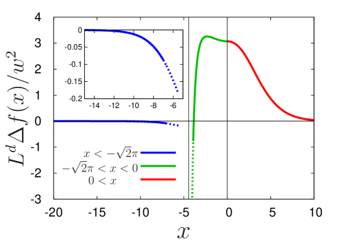
Figure 1: The scaling function $\Delta fL^{d}/w^{2}$ of the contribution to the critical Casimir force due to random surface fields as given by Eqs. (34) and (35). The underlying Gaussian approximation is evaluated for $d=4$, for which it is exact. The scaling variable $x$ equals $-L/\xi_{-}$ for $T\leq T_{c,bulk}$ and $+L/\xi_{+}$ for $T\geq T_{c,bulk}$. Withing mean field theory the critical temperature $T_{c,film}(L)$ corresponds to $x_{c}=-\sqrt{2}\,\pi$. The left vertical line corresponds to $x=x_{c}=-\sqrt{2}\pi$ whereas the right vertical line denotes $x=0$, i.e., the bulk critical point. The inset shows the magnified part of $\Delta fL^{d}/w^{2}$ as it is given by Eq. (34).

By inserting Eq. (27) into Eq. (26) and rearranging the integrand one obtains

$$\frac{\Delta F}{S_{d-1}}\;=\;\frac{h^{2}}{2c}\int\frac{d^{d-1}p}{(2\pi)^{d-1}}\Biggl{(}\frac{1-g_{1}}{2cg+1-g_{1}}\;-\;1\Biggr{)}\;.$$ (30)

In the next step, we insert the explicit expressions for $g$ and $g_{1}$ (Eqs. (28) and (29)) and determine the surface terms by taking the limit $x_{-}=L/\xi_{-}\to\infty$. Subtracting these $L$-independent terms we obtain the excess free energy (denoted by $\Delta\tilde{F}$)

$$\frac{\Delta\tilde{F}}{S_{d-1}} = \frac{h^{2}}{2c^{2}}\int\frac{d^{d-1}p}{(2\pi)^{d-1}}\sqrt{p^{2}+\xi_{-}^{-2}}\,\tanh\Bigl{(}\frac{L}{2}\sqrt{p^{2}+\xi_{-}^{-2}}\Bigr{)}\times$$ (31)

$$\times \Biggl{[}1\;-\;\frac{3}{2\sqrt{(p\xi_{-})^{2}+1}}\int_{0}^{x_{-}/2}ds\;\cosh^{-2}(s)\;\exp\Bigl{\{}-s\sqrt{(p\xi_{-})^{2}+1}\Bigr{\}}\Biggr{]}\,.$$

This expression is valid for large $c$ to leading order in an expansion in terms of $1/c$. Using the substitution $p=y/\xi_{-}$ and integrating over the angular part of the momenta, we obtain

$$\frac{\Delta\tilde{F}}{S_{d-1}} = \frac{\pi^{\frac{1-d}{2}}}{\Gamma\bigl{(}\frac{d+1}{2}\bigr{)}}\,\frac{h^{2}}{2c^{2}\xi_{-}^{d}}\;\int_{0}^{\infty}dy\;y^{d-2}\sqrt{y^{2}+1}\tanh\Bigl{(}\frac{x_{-}}{2}\sqrt{1+y^{2}}\Bigr{)}\times$$ (32)

$$\times \Biggl{[}1\;-\;\frac{3}{2\sqrt{y^{2}+1}}\int_{0}^{x_{-}/2}ds\;\cosh^{-2}(s)\;\exp\Bigl{\{}-s\sqrt{y^{2}+1}\Bigr{\}}\Biggr{]}\,.$$

Taking the negative derivative of this expression with respect to $L$, which amounts to $-\frac{\partial}{\partial L}=-\xi_{-}^{-1}\frac{\partial}{\partial x_{-}}$, renders the critical Casimir force $\Delta f$, per $k_{B}T$ and per area $S_{d-1}$, in excess to its value without random fields:

$$\Delta f \simeq -\frac{\pi^{\frac{1-d}{2}}}{\Gamma\bigl{(}\frac{d+1}{2}\bigr{)}}\,\frac{h^{2}}{4c^{2}\xi_{-}^{d+1}}$$ (33)

$$\int_{0}^{\infty}dy\;y^{d-2}\Biggl{\{}\frac{y^{2}+1}{\cosh^{2}\Bigl{[}\frac{x_{-}}{2}\sqrt{1+y^{2}}\Bigr{]}}\Biggl{[}1-\frac{3}{2\sqrt{y^{2}+1}}\int_{0}^{x_{-}/2}ds\frac{\exp\Bigl{(}-s\sqrt{y^{2}+1}\Bigr{)}}{\cosh^{2}(s)}\Biggr{]}\;-\;$$

$$- \frac{3\tanh\Bigl{(}\frac{x_{-}}{2}\sqrt{1+y^{2}}\Bigr{)}\exp\Bigl{(}-\frac{1}{2}x_{-}\sqrt{y^{2}+1}\Bigr{)}}{2\cosh^{2}\bigl{(}\frac{1}{2}x_{-}\bigr{)}}\Biggr{\}}\,.$$

Replacing $\xi_{-}$ by $L/x_{-}$ and identifying the dimensionless scaling variable $w^{2}=h^{2}/(c^{2}L)$ (see Introduction), leads to the following final result:

$$\Delta f \simeq -\mathcal{A}(d)\frac{w^{2}x_{-}^{d+1}}{L^{d}}\int_{0}^{\infty}dy\;y^{d-2}\times$$ (34)

$$\times \Biggl{\{}\frac{y^{2}+1}{\cosh^{2}\Bigl{[}\frac{x_{-}}{2}\sqrt{1+y^{2}}\Bigr{]}}\Biggl{(}1-\frac{3}{2\sqrt{y^{2}+1}}\int_{0}^{x_{-}/2}ds\frac{\exp\Bigl{[}-s\sqrt{y^{2}+1}\Bigr{]}}{\cosh^{2}(s)}\Biggr{)}$$

$$- \frac{3\tanh\Bigl{(}\frac{x_{-}}{2}\sqrt{1+y^{2}}\Bigr{)}\exp\Bigl{[}-\frac{1}{2}x_{-}\sqrt{y^{2}+1}\Bigr{]}}{2\cosh^{2}\bigl{(}\frac{1}{2}x_{-}\bigr{)}}\Biggr{\}}$$

which is valid for $x_{-}\gg 1$ , $c\gg 1$ (to leading order $O(1/c^{3})$; compare Eqs. (12) and (13)). The prefactor is given by $\mathcal{A}(d)=\pi^{\frac{1-d}{2}}/(4\Gamma\bigl{(}\frac{d+1}{2}\bigr{)})$ .

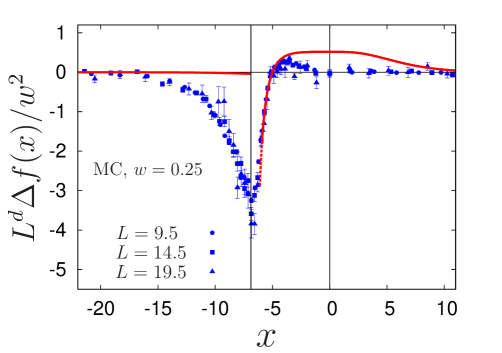
Figure 2: The scaling function $\Delta fL^{3}/w^{2}$ of the contribution to the critical Casimir force due to random surface fields calculated within Gaussian approximation in $d=3$ and given by Eqs. (34) and (35). These results are compared with Monte Carlo (MC) simulations data or the $3d$ Ising film with random surface fields taken from Fig. 3(b) in Ref. MVDD . In order to obtain the best fit, the analytic results have been rescaled as follows: $x\to 1.55x$, $y\to 0.3y$. For the $3d$ Ising model the random surface field scaling variable is $\hat{w}=h/L^{0.26}$ (see Eq. (2)). The vertical lines indicate $T_{c,bulk}$ and $T_{c,film}(L)$ within MFT, corresponding to $x=0$ and $x=-6.88$, respectively. Concerning the reason for the discrepancy between the MC data and the analytic result below $x\lesssim-6.88$ see the main text after Eq. (35).

Analogous calculations (see Appendix B) for the contribution of random surface fields to the critical Casimir force in the disordered film phase for $-\pi^{2}/L^{2}=\;\tau_{c}<\tau<0$ and for $\tau>0$ yield

$$\Delta f=-\frac{\mathcal{A}(d)w^{2}}{L^{d}}\left\{\begin{array}[]{ll}\int_{0}^{1}dy\frac{x_{-}^{d+1}y^{d-2}(1-y^{2})}{2^{(d+1)/2}\cos^{2}\Bigl{(}\frac{x_{-}}{2\sqrt{2}}\sqrt{1-y^{2}}\Bigr{)}}\\ -\int_{1}^{\infty}dy\frac{x_{-}^{d+1}y^{d-2}(y^{2}-1)}{2^{(d+1)/2}\cosh^{2}\Bigl{(}\frac{x_{-}}{2\sqrt{2}}\sqrt{y^{2}-1}\Bigr{)}},\;-\sqrt{2}\pi<-x_{-}\leq 0\\ \\ -\int_{0}^{\infty}dy\frac{x_{+}^{d+1}y^{d-2}(y^{2}+1)}{\cosh^{2}\Bigl{(}\frac{x_{+}}{2}\sqrt{y^{2}+1}\Bigr{)}},\;\;\;x_{+}\geq 0\end{array}\right.$$ (35)

where $x_{-}=-L/\xi_{-}$ and $x_{+}=L/\xi_{+}$. Note that because in the disordered phase the mean field OP profile $\psi_{-}(s,x_{-})$ is identically equal to zero, the derivation of the above result turns out to be much more simple than the one for the ordered phase in Eq. (34). Whereas Eq. ( 34) is only approximately valid for $x_{-}\gg 1$, i.e., $x=-x_{-}\to-\infty$, Eq. (35) holds for $0>-x_{-}\gtrsim-\sqrt{2}\pi$, i.e., not too close to $\tau_{c}$, and for $x_{+}=L/\xi_{+}\geq 0$. The scaling function $\Delta fL^{d}/w^{2}$ of the random field contribution to the critical Casimir force as given by Eqs. (34) and (35) is shown in Fig. 1.

V Discussion and perspectives

It is interesting and instructive to compare the qualitative behavior of the contribution to the critical Casimir force due to random surface fields with the corresponding force for the pure system with Dirichlet-Dirichlet boundary conditions. In the absence of random surface fields (i.e., $h=0$) the free energy is given by the first two terms on the r.h.s. of Eq. (23). There, the first term is the standard mean field contribution (Eq. (6)), while the second term stems from the Gaussian fluctuations described by the correlation function matrix given in Eq. (10). Accordingly one finds for the CCF $f_{0}$ (per $k_{B}T$ and per area $S_{d-1}$ and in excess of the $L$-independent contribution from the bulk free energy) $f_{0}=-(\partial E_{0}/\partial L)+f_{0}^{(G)}$, where $f_{0}^{(G)}$ is the contribution from the Gaussian fluctuations. (The surface free energy of the film does not depend on the film thickness and thus it does not render a contribution to $f_{0}$.) An analytical expression for the mean field contribution $-\partial E_{0}/\partial L$ is available only for $d=4$; it is given by Eq. (56) and Fig. 9 in Ref. mgd . This result vanishes $\sim|x_{-}|^{2}\exp(-\sqrt{2}|x_{-}|)$ for $-x_{-}\to-\infty$, is parabolic for $-\sqrt{2}\pi\leq-x_{-}\leq 0$, and is zero for $x_{+}>0$. For $T<T_{c,b}$ the Gaussian contribution $f_{0}^{(G)}$ must be determined numerically (second term in Eq. (23)). For $T>T_{c,b}$ one has $f_{0}^{(G)}(x_{+}>0,d=4)=3\Theta_{+(0,0)}(x_{+})-x_{+}\Theta^{\prime}_{+(0,0)}(x_{+})$ with $\Theta_{+(0,0)}(x_{+})=-\bigl{(}x_{+}^{4}/(6\pi^{2})\bigr{)}\int_{1}^{\infty}dy(y^{2}-1)^{3/2}/(e^{2x_{+}y}-1)$ (see Eq. (6.12) for $\epsilon=0$ in the first entry of Ref. dietrich_krech ); accordingly $f_{0}^{(G)}(x_{+}\to\infty)=-\bigl{(}1/(16\pi^{3/2})\bigr{)}x_{+}^{3/2}e^{-2x_{+}}$. For $d=3$, the numerically evaluated mean field contribution is shown in Fig. 13 of Ref. VGMD . For $d=3$ and $T<T_{c,b}$, as for $d=4$, the Gaussian contribution $f_{0}^{(G)}$ must be determined numerically. For $d=3$ and $T>T_{c,b}$ one has $f_{0}^{(G)}(x_{+}>0,d=3)=3\Theta_{+(0,0)}(x_{+})-x_{+}\Theta^{\prime}_{+(0,0)}(x_{+})$ with $\Theta_{+(0,0)}(x_{+})=-x_{+}^{3/(4\pi)}\int_{1}^{\infty}dy(y^{2}-1)/(e^{2x_{+}y}-1)$ (see Eq. (6.6) in the first entry of Ref. dietrich_krech ); accordingly $f_{0}^{(G)}(x_{+}\to\infty)=-\bigl{(}1/(6\pi)\bigr{)}x_{+}e^{-2x_{+}}$.

Our results obtained within the Gaussian approximation for weak disorder in $d=3$ (Eqs. (34)) confirm the the interpretation of the MC simulation data in Ref. MVDD , formulated therein as a hypothesis. This hypothesis states that for small values of $w$ the contribution $\Delta f$ to the critical Casimir force due to random surface fields is, to leading order, proportional to $w^{2}$, i.e., for the scaling function $\vartheta$ of the critical Casimir force one has

$$f_{0}(T,L,h)L^{3}=\vartheta(x,w)\approx\vartheta(x,w=0)+w^{2}\delta\vartheta(x)\,,$$ (36)

where $\vartheta(x,w=0)$ is the scaling function of the critical Casimir force for $(o,o)$ BC without RSF and the universal scaling function $\delta\vartheta$, which is defined via Eq. (36), depends on $x$ only. The scaling variable $x$ equals $-L/\xi_{-}$ for $T\leq T_{c,b}$ and $+L/\xi_{+}$ for $T\geq T_{c,b}$. In Fig. 2, we compare $\Delta fL^{d}/w^{2}=L^{d}(f_{0}(T,L,h)-f_{0}(T,L,h=0))/w^{2}\;\simeq\delta\vartheta(x)$ as given by Eqs. (34) and (35) for $d=3$ with the MC simulation data obtained in Ref. MVDD for $3d$ Ising films with weak surface disorder corresponding to the scaling variable $\hat{w}=h/L^{0.26}=0.25$. (In the Ising model considered in Ref. MVDD , the coupling constant within the surface layers and between the surface layers and their neighboring layers has been taken to be the same as in the bulk. The corresponding surface enhancement is, within mean-field theory and in units of the lattice spacing, $c=1$ binder . Beyond mean field theory, the relation between $c$ and the coupling constants is not known. In Ref. MVDD the value of $c$ has been set such that $c^{0.87}=1/\kappa$ and the scaling variable $\hat{w}=h/L^{0.26}$ has been used.) The best fit of the MC data by the analytical result is achieved by stretching and compressing the scaling variable $x$ and the amplitude of the analytic result for $\Delta fL^{d}/w^{2}$ by a factor of $1.55$ and of $0.3$, respectively. As can be inferred from Fig. 2, the Gaussian approximation qualitatively captures the influence of the random surface fields on the CCF in the case of weak disorder. Quantitative agreement is not expected and, indeed, we find that for $-15\lesssim x\lesssim 10$ the analytic result for $d=3$ deviates from the MC data. The observed discrepancy is enhanced by the fact that the analytic calculations have been performed by assuming the limit $c\to\infty$, whereas the MC simulation data have been obtained for $c\simeq 1$. Moreover, for $x<x_{c}=-\sqrt{2}\pi$, the scaling function for the OP profile has been approximated by the scaling function for the associated semi-infinite system close to its fixed-point form corresponding to $c=\infty$ (compare Eqs. (12) and (13)). As already discussed earlier (see Section II, Eqs. (12) and (13)), this approximation is valid for $x_{-}\gg 1$. As can be seen in Fig. 3, for $c=1$, which corresponds to the model system studied within the MC simulation, even for $x_{-}$ as large as 20 the deviation of the OP scaling function for a film from the one for the corresponding semi-infinite system is considerable. The smaller the film thickness, the stronger is the deviation.

Concerning future studies, it would be desirable to consider spatially correlated random surface fields with nonzero mean which better mimic the actual physical systems. In addition, it would be interesting to study to which extent random surface fields eliminate the critical point $T_{c,film}$ of the film and, if not, how $T_{c,film}$ is shifted by the Gaussian fluctuations with and without random surface fields.

Finally it would be rewarding to make analytic progress beyond the Gaussian approximation. To this end one can extend the renormalization group analysis for the energy density at a single surface (i.e., for a semi-infinite system DD ) to that in the presence of a second surface at a distance $L$ (i.e., for the film geometry). This will lead to a scaling form of the surface energy density which is complicated due to the combination of multiplicative and additive renormalization. Even the comparison of this scaling property with the present explicit Gaussian result is expected to be impeded by logarithmic corrections appearing in $d=4$. Moreover, in order to be consistent the relation in Eq. (26) has to be augmented in order to capture non-Gaussian contributions.

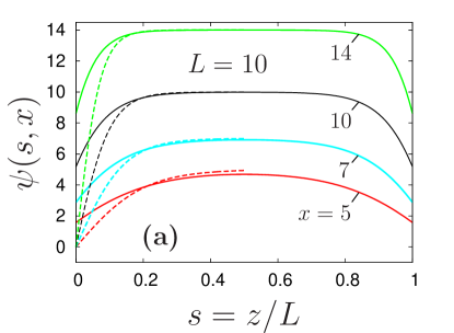
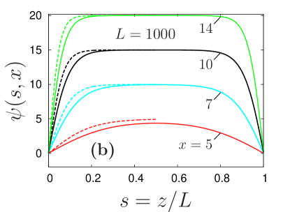
Figure 3: Scaling function $\psi(s,x)$ of the OP profile in the film (see Sec. III) of thickness $L=10$ (a) and $L=1000$ (b) with $(o,o)$ BCs for various values of the scaling variable $x_{-}=L/\xi_{-}$ (solid lines) as obtained within mean field theory for $c=1$ (see Ref. Gambassi_Dietrich ) compared with the ones for the corresponding semi-infinite system at the fixed point $c=\infty$ (dashed lines). For the narrow film with $L=10$, deviations from the semi-infinite OP scaling function are more pronounced and occur at smaller values of $x_{-}$ as for the thick films. Such narrow films have been studied by the MC simulations reported in Ref. MVDD .

Acknowledgments: The work by AM has been supported by the Polish National Science Center (Harmonia Grant No. 2015/18/M/ST3/00403).

Appendix A: ordered phase in the film

In this appendix we consider the Gaussian fluctuations around a nonzero mean field order parameter $\phi_{*}\not=0$. This occurs at $\tau<\tau_{c}=-\pi^{2}/L^{2}$, i.e., below the bulk critical point Gambassi_Dietrich . In terms of the scaling variable $x(\tau<0)=-x_{-}$ this appendix is concerned with $x<\sqrt{2}\pi$.

Accordingly, due to to Eqs. (10) and (14) the matrix elements $G_{l,l^{\prime}}^{-1}$ are given as

$$G_{l,l^{\prime}}^{-1}\;=\;a_{l}\delta_{l,-l^{\prime}}-\tilde{m}(l+l^{\prime};x_{-})+2c$$ (A1)

where

$$a_{l}=L\Bigl{[}p^{2}+\xi_{-}^{-2}+\Bigl{(}\frac{2\pi l}{L}\Bigr{)}^{2}\Bigr{]}$$ (A2)

and approximately

$$\tilde{m}(l;x_{-})=\frac{3}{\xi_{-}}\int_{0}^{x_{-}/2}ds\;\cosh^{-2}(s)\cos\Bigl{(}\frac{2\pi l}{x_{-}}s\Bigr{)}$$ (A3)

In view of Eq. (26) our aim is to compute the quantity

$$S\;=\;\sum_{l,l^{\prime}=-\infty}^{+\infty}G_{l,l^{\prime}}$$ (A4)

where the matrix $\hat{G}=\bigl{(}G_{l,l^{\prime}}\bigr{)}$ is the inverse of the matrix $\hat{G}^{-1}=\bigl{(}G_{l,l^{\prime}}^{-1}\bigr{)}$ given by Eq. (A1). It will turn out that the above sum $S$ can be computed without making use of an explicit expression for the matrix elements $G_{l,l^{\prime}}$.

To start with, we consider the matrices $G_{l,l^{\prime}}$ and $G_{l,l^{\prime}}^{-1}$ to have a very large but finite rank $N\times N$; only in the final result we shall take the limit $N\to\infty$. By definition the inverse matrix fulfills

$$\sum_{l^{\prime}=-N}^{N}G_{l_{1},l^{\prime}}^{-1}\,G_{l^{\prime},l_{2}}\;=\;\delta_{l_{1},l_{2}}\;.$$ (A5)

Summing the above relation over $l_{1}$ and $l_{2}$ we find

$$\sum_{l=-N}^{N}\tilde{C}_{l}\,C_{l}\;=\;2N+1$$ (A6)

where

$$C_{l}\;=\;\sum_{l^{\prime}=-N}^{N}G_{l,l^{\prime}}\;$$ (A7)

and, according to Eq. (A1),

$$\tilde{C}_{l}=\sum_{l^{\prime}=-N}^{N}G_{l,l^{\prime}}^{-1} = \sum_{l^{\prime}=-N}^{N}\Bigl{[}a_{l}\delta_{l,-l^{\prime}}-\tilde{m}(l+l^{\prime};x_{-})+2c\Bigr{]}$$ (A8)

$$= a_{l}-M(x_{-},l)+2c(2N+1)$$

where

$$M(x_{-},l)\;=\;\sum_{l^{\prime}=-N}^{N}\tilde{m}(l+l^{\prime};x_{-})\;=\;\frac{3}{\xi_{-}}\sum_{l^{\prime\prime}=-N+l}^{N+l}\int_{0}^{x_{-}/2}ds\;\cosh^{-2}(s)\cos\Bigl{(}\frac{2\pi l^{\prime\prime}}{x_{-}}s\Bigr{)}.$$ (A9)

$M(x_{-},l)$ can be written as

$$M(x_{-},l)\; = M(x_{-})+R(l;x_{-})\;=\;\sum_{l^{\prime}=-N}^{N}\tilde{m}(l^{\prime};x_{-})+R(l;N;x_{-})$$

$$= \;\frac{3}{\xi_{-}}\sum_{l^{\prime\prime}=-N}^{N}\int_{0}^{x_{-}/2}ds\;\cosh^{-2}(s)\cos\Bigl{(}\frac{2\pi l^{\prime\prime}}{x_{-}}s\Bigr{)}+R(l;N;x_{-})$$ (A10)

with $M(x_{-})=M(x_{-},l=0)$. In the limit of large $N$ (which will be taken to infinity in the final result) one has $R(l;N\to\infty;x_{-})=0$ for all $l$ and $x_{-}$. Substituting Eq. (A8) into Eq. (A6) and taking into account that according to the definition in Eq. (A4), one has $S=\sum_{l}C_{l}$ so that

$$\sum_{l=-N}^{N}\Bigl{(}a_{l}-R(l;N;x_{-})\Bigr{)}C_{l}+\Bigl{(}(4N+2)c-M(x_{-})\Bigr{)}\,S\;=\;2N+1.$$ (A11)

This equation is satisfied by

$$C_{l}\;=\;\Bigl{(}a_{l}-R(l;N;x_{-})\Bigr{)}^{-1}\Bigl{[}1+\tilde{m}(l;x_{-})S-2cS\Bigr{]}\;.$$ (A12)

Summing Eq. (A12) over $l$ we obtain a simple equation for $S$:

$$S\;=\;\sum_{l=-N}^{N}\Bigl{(}a_{l}-R(l;N;x_{-})\Bigr{)}^{-1}\;+\;S\sum_{l=-N}^{N}\frac{\tilde{m}(l;x_{-})}{a_{l}-R(l;N;x_{-})}\;-\;2cS\sum_{l=-N}^{N}\frac{1}{a_{l}-R(l;N;x_{-})}\,.$$ (A13)

In the limit $N\to\infty$ we eventually find

$$\sum_{l,l^{\prime}=-\infty}^{+\infty}G_{l,l^{\prime}}\;\equiv\;S\;=\;\frac{g}{1\;+\;2c\,g\;-g_{1}}$$ (A14)

which is Eq. (27). The series

$$g\;=\;\sum_{l=-\infty}^{+\infty}a_{l}^{-1}$$ (A15)

and

$$g_{1}\;=\;\sum_{l=-\infty}^{+\infty}a_{l}^{-1}\;\tilde{m}(l;x_{-})$$ (A16)

are still to be calculated.

With Eq. (A2) the series in Eq. (A15) can be written as

$$g\;=\;\frac{L}{4\pi^{2}}\Bigl{[}2\sum_{l=1}^{\infty}\frac{1}{l^{2}+\gamma^{2}}+\frac{1}{\gamma^{2}}\Bigr{]}\;,$$ (A17)

where

$$\gamma^{2}=\frac{L^{2}}{4\pi^{2}}\bigl{(}p^{2}+\xi_{-}^{-2}\bigr{)}\;=\;\frac{x_{-}^{2}}{4\pi^{2}}\;\bigl{[}(\xi_{-}p)^{2}+1\bigr{]}.$$ (A18)

The series in Eq. (A17) is known as $\sum_{l=1}^{\infty}(l^{2}+\gamma^{2})^{-1}=\frac{\pi}{2\gamma}[\tanh(\pi\gamma)]^{-1}-\frac{1}{2\gamma^{2}}$ (see Eq. (1.217.1) in Ref. Grandshteyn ). Thus we obtain

$$g\;\equiv\;g(p,L,\xi_{-})\;=\;\frac{1}{2\sqrt{p^{2}+\xi^{-2}_{-}}\tanh\Bigl{(}\frac{L}{2}\sqrt{p^{2}+\xi_{-}^{-2}}\Bigr{)}}\;,$$ (A19)

which is Eq. (28).

The series in Eq. (A16) can be written as

$$g_{1}\;=\;\frac{3L}{4\pi^{2}\xi_{-}}\int_{0}^{x_{-}/2}ds\;\cosh^{-2}(s)\sum_{l=-\infty}^{+\infty}\frac{1}{l^{2}+\gamma^{2}}\cos\Bigl{(}\frac{2\pi l}{x_{-}}s\Bigr{)}\,.$$ (A20)

For large values of $x_{-}$ the series in Eq. (A20) can be approximated by the integral

$$g_{1} = \frac{3}{4\pi^{2}}\int_{0}^{x_{-}/2}ds\;\cosh^{-2}(s)\frac{1}{x_{-}}\sum_{l=-\infty}^{+\infty}\frac{1}{\Bigl{(}\frac{l}{x_{-}}\Bigr{)}^{2}+\frac{1}{4\pi^{2}}\;\bigl{[}(p\xi_{-})^{2}+1\bigr{]}}\cos\Bigl{(}2\pi s\frac{l}{x_{-}}\Bigr{)}$$ (A21)

$$\simeq \frac{3}{4\pi^{2}}\int_{0}^{x_{-}/2}ds\;\cosh^{-2}(s)\;\int_{-\infty}^{+\infty}dt\frac{1}{t^{2}+\frac{1}{4\pi^{2}}\;\bigl{[}(p\xi_{-})^{2}+1\bigr{]}}\cos\Bigl{(}2\pi s\;t\Bigr{)}.$$

Simple integration over $t$ yields

$$g_{1}\equiv g_{1}\bigl{(}(p\xi_{-})^{2},x_{-}\bigr{)}\;=\;\frac{3}{2\sqrt{(p\xi_{-})^{2}+1}}\int_{0}^{x_{-}/2}ds\;\cosh^{-2}(s)\;\exp\Bigl{\{}-s\sqrt{(p\xi_{-})^{2}+1}\Bigr{\}}.$$ (A22)

Appendix B: disordered phase in the film

B1: $-\pi^{2}/L^{2}<\tau\leq 0$

In the disordered phase in the film below $T_{c,bulk}$ (for which the mean field equilibrium profile is identically zero, i.e., $\phi_{*}(z)\equiv 0$ as for $T>T_{c,bulk}$) the Hamiltonian, which describes the fluctuating field $\varphi({\bf r},z)$ within the Gaussian approximation, is given by

$${\cal H}_{0}[\varphi]=+\frac{1}{2}\int d^{d-1}r\int_{0}^{L}dz\Bigl{[}\bigl{(}\nabla\varphi\bigr{)}^{2}-\frac{1}{2}\xi_{-}^{-2}\varphi^{2}+c\varphi^{2}\bigl{[}\delta(z)+\delta(z-L)\bigr{]}\Bigr{]}\;.$$ (B1)

With $-\frac{1}{2}\xi_{-}^{-2}=\tau\;$ Eq. (B1) holds for the interval $-\pi^{2}/L^{2}<\tau\leq 0$ in which the bulk is ordered but the film is disordered. Inserting the Fourier representation (Eq. (7)) into Eq. (B1) yields

$${\cal H}_{0}[\tilde{\varphi}]=\frac{1}{2}\int\frac{d^{d-1}p}{(2\pi)^{d-1}}\,\frac{1}{L^{2}}\sum_{l,l^{\prime}=-\infty}^{+\infty}G^{-1}_{l,l^{\prime}}(p)\,\tilde{\varphi}({\bf p},l)\tilde{\varphi}(-{\bf p},l^{\prime})$$ (B2)

where the matrix elements $G^{-1}_{l,l^{\prime}}(p)$ have a much more simple structure compared with the ones in Eq. (10):

$$G^{-1}_{l,l^{\prime}}(p)\;=\;L\Bigl{[}p^{2}-\frac{1}{2}\xi_{-}^{-2}+\frac{4\pi^{2}}{L^{2}}l^{2}\Bigr{]}\delta_{l,-l^{\prime}}\,+\,2c.$$ (B3)

Following the same steps as in the calculation for the ordered phase, for the free energy contribution $\Delta F(h,L)$, caused by the random fields, one obtains the analogue of Eq. (26) for which instead of Eq. (27) one now finds a much more simple expression:

$$\sum_{l,l^{\prime}=-\infty}^{+\infty}G_{l,l^{\prime}}(p)\;=\;\frac{g(p,L,\xi_{-})}{1+2c\,g(p,L,\xi_{-})}$$ (B4)

with

$$g(p,L,\xi_{-})\;=\;\frac{1}{L}\sum_{l=-\infty}^{+\infty}\Bigl{[}p^{2}-\frac{1}{2}\xi_{-}^{-2}+\Bigl{(}\frac{2\pi l}{L}\Bigr{)}^{2}\Bigr{]}^{-1}.$$ (B5)

Repeating the calculations carried out in Appendix A, which lead to the result in Eq. (A19), one finds for the domain $p^{2}>\frac{1}{2}\xi_{-}^{-2}$

$$g(p,L,\xi_{-})\Big{|}_{p^{2}>\frac{1}{2}\xi_{-}^{-2}}\;\equiv\;g_{+}(p,L,\xi_{-})\;=\;\frac{1}{2\sqrt{p^{2}-\frac{1}{2}\xi_{-}^{-2}}\,\tanh\Bigl{(}\frac{L}{2}\sqrt{p^{2}-\frac{1}{2}\xi_{-}^{-2}}\Bigr{)}}\;.$$ (B6)

Similar calculations for the domain $p^{2}<\frac{1}{2}\xi_{-}^{-2}$ yield

$$g(p,L,\xi_{-})\Big{|}_{p^{2}<\frac{1}{2}\xi_{-}^{-2}}\;\equiv\;g_{-}(p,L,\xi_{-})\;=\;-\frac{1}{2\sqrt{\frac{1}{2}\xi_{-}^{-2}-p^{2}}\,\tan\Bigl{(}\frac{L}{2}\sqrt{\frac{1}{2}\xi_{-}^{-2}-p^{2}}\Bigr{)}}\;.$$ (B7)

Upon inserting Eq. (B4) into Eq. (26) and subtracting $L$-independent terms, for large $c$, i.e., to leading order in an expansion in terms of $1/c$, we obtain for the corresponding excess free energy (denoted as $\Delta\tilde{F}$)

$$\frac{\Delta\tilde{F}}{S_{d-1}}\;=\;\frac{h^{2}}{4c^{2}}\Biggl{[}\int_{|{\bf p}|<\frac{1}{\sqrt{2}\,\xi_{-}}}\frac{d^{d-1}p}{(2\pi)^{d-1}}\;\frac{1}{g_{-}(p,L,\xi_{-})}+\int_{|{\bf p}|>\frac{1}{\sqrt{2}\,\xi_{-}}}\frac{d^{d-1}p}{(2\pi)^{d-1}}\;\frac{1}{g_{+}(p,L,\xi_{-})}\Biggr{]}\,.$$ (B8)

Substituting here Eqs. (B6) and (B7) respectively, changing the integration variable according to $p=y/\sqrt{2}\xi_{-}$, and integrating over the angular part of the momenta we obtain

$$\frac{\Delta\tilde{F}}{S_{d-1}} = \frac{\pi^{\frac{1-d}{2}}h^{2}}{2\Gamma\bigl{(}\frac{d+1}{2}\bigr{)}c^{2}(\sqrt{2}\xi_{-})^{d}}\Biggl{[}-\int_{0}^{1}dy\sqrt{1-y^{2}}\tan\Bigl{(}\frac{x_{-}}{2\sqrt{2}}\sqrt{1-y^{2}}\Bigr{)}\;+$$ (B9)

$$+ \int_{1}^{\infty}dy\sqrt{y^{2}-1}\tanh\Bigl{(}\frac{x_{-}}{2\sqrt{2}}\sqrt{y^{2}-1}\Bigr{)}\Biggr{]}\,.$$

Taking the negative derivative of this expression with respect to $L$, $-\frac{\partial}{\partial L}=-\xi_{-}^{-1}\frac{\partial}{\partial x_{-}}$ renders the critical Casimir force $\Delta f$, per $k_{B}T$ and per area $S_{d-1}$, in excess to its value without random fields:

$$\Delta f\,=\,-\frac{\pi^{\frac{1-d}{2}}}{4\Gamma\bigl{(}\frac{d+1}{2}\bigr{)}}\;\frac{w^{2}x_{-}^{d+1}}{L^{d}2^{(d+1)/2}}\;\Biggl{[}\int_{0}^{1}dy\frac{y^{d-2}(1-y^{2})}{\cos^{2}\Bigl{(}\frac{x_{-}}{2\sqrt{2}}\sqrt{1-y^{2}}\Bigr{)}}\;-\;\int_{1}^{\infty}dy\frac{y^{d-2}(y^{2}-1)}{\cosh^{2}\Bigl{(}\frac{x_{-}}{2\sqrt{2}}\sqrt{y^{2}-1}\Bigr{)}}\Biggr{]}\;,$$ (B10)

which is valid for $-\pi^{2}/L^{2}<\tau\leq 0$ or equivalently for $-\sqrt{2}\,\pi<-x_{-}\leq 0$.

B2: $\tau>0$

For $\tau>0$ the Gaussian Hamiltonian for the fluctuating fields is (with $\xi_{+}^{-2}=\tau$)

$${\cal H}_{0}[\varphi]=+\frac{1}{2}\int d^{d-1}r\int_{0}^{L}dz\Bigl{[}\bigl{(}\nabla\varphi\bigr{)}^{2}+\xi_{+}^{-2}\varphi^{2}+c\varphi^{2}\bigl{[}\delta(z)+\delta(z-L)\bigr{]}\Bigr{]}\;.$$ (B11)

Correspondingly, in the Fourier representation (Eq. (7)) one obtains

$${\cal H}_{0}[\tilde{\varphi}]=\frac{1}{2}\int\frac{d^{d-1}p}{(2\pi)^{d-1}}\,\frac{1}{L^{2}}\sum_{l,l^{\prime}=-\infty}^{+\infty}G^{-1}_{l,l^{\prime}}(p)\,\tilde{\varphi}({\bf p},l)\tilde{\varphi}(-{\bf p},l^{\prime})$$ (B12)

where

$$G^{-1}_{l,l^{\prime}}(p)\;=\;L\Bigl{[}p^{2}+\xi_{+}^{-2}+\frac{4\pi^{2}}{L^{2}}l^{2}\Bigr{]}\delta_{l,-l^{\prime}}\,+\,2c\;.$$ (B13)

Following the same steps as above, for the free energy contribution $\Delta F(h,L)$ due to the random fields one finds Eq. (26) where

$$\sum_{l,l^{\prime}=-\infty}^{+\infty}G_{l,l^{\prime}}(p)\;=\;\frac{g(p,L,\xi_{+})}{1+2c\,g(p,L,\xi_{+})}$$ (B14)

with

$$g(p,L,\xi_{+})\;=\;\frac{1}{L}\sum_{l=-\infty}^{+\infty}\Bigl{[}p^{2}+\xi_{+}^{-2}+\Bigl{(}\frac{2\pi l}{L}\Bigr{)}^{2}\Bigr{]}^{-1}\;=\;\frac{1}{2\sqrt{p^{2}+\xi_{+}^{-2}}\,\tanh\Bigl{(}\frac{L}{2}\sqrt{p^{2}+\xi_{+}^{-2}}\Bigr{)}}\;.$$ (B15)

For $\tau>0$, this yields the expression analogous to Eq. (B10) for the critical Casimir force in excess to its value without random fields:

$$\Delta f\,=\,\frac{\pi^{\frac{1-d}{2}}}{4\Gamma\bigl{(}\frac{d+1}{2}\bigr{)}}\;\frac{w^{2}x_{+}^{d+1}}{L^{d}}\;\int_{0}^{\infty}dy\frac{y^{d-2}(y^{2}+1)}{\cosh^{2}\Bigl{(}\frac{x_{+}}{2}\sqrt{y^{2}+1}\Bigr{)}}\;,$$ (B16)

which is valid for $x_{+}>0$.

References

(1) M. E. Fisher and P. G. de Gennes, C. R. Seances Acad. Sci., Ser. B 287, 207 (1978).
(2)
H. B. Casimir H. B., Proc. K. Ned. Akad. Wet. 51, 793 (1948).
(3) M. Krech, Casimir Effect in Critical Systems (World Scientific, Singapore, 1994);
J. Phys.: Condens. Matter 11, R391 (1999);
M. Kardar and R. Golestanian, Rev. Mod. Phys. 71, 1233 (1999);
A. Gambassi, J. Phys.: Conf. Ser. 161, 012037 (2009).
(4)
K. Binder, in Phase Transitions and Critical Phenomena, edited by C. Domb and J. L. Lebowitz
(Academic, New York, 1983), Vol. 8, p. 1; H. W. Diehl, ibid. Vol. 10 (1986) p. 76.
(5) M. Fukuto, Y. F. Yano, and P. S. Pershan, Phys. Rev. Lett. 94, 135702 (2005).
(6) S. Rafaï S., D. Bonn, and J. Meunier, Physica A 386, 31 (2007).
(7) C. Hertlein, L. Helden, A. Gambassi, S. Dietrich, and C. Bechinger, Nature 451, 172 (2008).
(8)
A. Gambassi, A. Maciołek, C. Hertlein, U. Nellen, L. Helden, C. Bechinger, and S. Dietrich, Phys. Rev. E 80, 061143 (2009).
(9)
U. Nellen, J. Dietrich, L. Helden, S. Chodankar, K. Nygard, J. F. van der Veen, and C. Bechinger, Soft Matter 7, 5360 (2011).
(10) R. Garcia and M. H. W. Chan, Phys. Rev. Lett. 83, 1187 (1999);
A. Ganshin, S. Scheidemantel, R. Garcia, and M. H.W. Chan,
ibid.97, 075301 (2006).
(11) R. Garcia and M. H. W. Chan, Phys. Rev. Lett. 88, 086101 (2002).
(12) M. Krech and S. Dietrich, Phys. Rev. A 46, 1886 (1992); ibid.46, 1922 (1992).
(13) M. Krech, Phys. Rev. E 56, 1642 (1997).
(14) Z. Borjan and P. J. Upton, Phys. Rev. Lett. 81, 4911 (1998); ibid.101, 125702 (2008).
(15) Z. Borjan, EPL 99, 56004 (2012).
(16) A. Maciołek and S. Dietrich, Europhys. Lett. 74, 22 (2006).
(17) (a) O. Vasilyev, A. Gambassi, A. Maciołek, and S. Dietrich, EPL 80, 60009 (2007); (b)
Phys. Rev. E 79, 041142 (2009).
(18) A. Hucht, Phys. Rev. Lett. 99, 185301 (2007).
(19) M. Hasenbusch, Phys. Rev. B 82, 104425 (2010).
(20) U. Nellen, L. Helden, and C. Bechinger, EPL 88, 26001 (2009).
(21) T. F. Mohry, A. Maciołek, and S. Dietrich, Phys. Rev. E 81, 061117 (2010).
(22) D. B. Abraham and A. Maciołek, Phys. Rev. Lett. 105, 055701 (2010).
(23) O. Vasilyev, A. Maciołek, and S. Dietrich, Phys. Rev. E 84, 041605 (2011).
(24) F. M. Schmidt and H. W. Diehl, Phys. Rev. Lett. 101, 100601 (2008).
(25) M. Tröndle, O. Zvyagolskaya, A. Gambassi, D. Vogt, L. Harnau, C. Bechinger, and S. Dietrich, Mol. Phys. 109, 1169 (2011).
(26) A. Naji, D. S. Dean, J. Sarabadani, R. R. Horgan, and R. Podgornik, Phys. Rev. Lett. 104, 060601 (2010).
(27) D. Ben-Yaakov, D. Andelman, and H. Diamant, Phys. Rev. E 87, 022402 (2013).
(28) A. Maciołek, O. Vasilyev, V. Dotsenko, and S. Dietrich, Phys. Rev. E 91, 032408 (2015).
(29) F. Parisen Toldin, Phys. Rev. E 91, 032105 (2015).
(30) M. Blume, Phys. Rev. 141, 517 (1966).
(31) H. W. Capel, Physica 32, 966 (1966).
(32) H. W. Diehl and A. Nüsser, Z. Phys. B 79, 69 (1990).
(33) K. K. Mon and M. P. Nightingale, Phys. Rev. B 37, 3815 (1988).
(34) S. Dietrich, in Phase Transitions and Critical Phenomena, edited by C. Domb and J. L. Lebowitz, Vol. 12
(Academic, London, 1988), p.1;
G. Forgacs, R. Lipowsky, and T. M. Nieuwenhuizen, ibid. Vol. 14 (1991), p. 135.
(35) F. Iglói, L. Turban, and B. Berche, J. Phys. A: Math. Gen. 24, L1031 (1991).
(36) J. L. Cardy, J. Phys. A: Math. Gen. 24, L1315 (1991).
(37) M. Pleimling, J. Phys. A: Math. Gen. 37, R79 (2004).
(38) F. Karimi Pour Haddadan, A. Naji, A. Khame Seifi, and R. Podgornik, J. Phys.: Condens. Matter 26, 075103 (2014).
(39) R. Guida and J. Zinn Justin, J. Phys. A: Math. Gen. 31, 8103 (1998).
(40) A. Pelissetto and E. Vicari, Phys. Rep. 368, 549 (2002).
(41) M. Hasenbusch, Phys. Rev. B 84, 134405 (2011); ibid.83, 134425 (2011).
(42) A. Gambassi and S. Dietrich, J. Stat. Phys. 123, 929 (2006).
(43) H. W. Diehl H. W., Int. J. Mod. Phys. B 11, 3503 (1997).
(44) S. Z. Lin and B. Zheng, Phys. Rev. E 78, 011127 (2008).
(45) S. Dietrich and H. W. Diehl, Z. Phys. B 43, 315 (1981).
(46) M. Krech, E. Eisenriegler, and S. Dietrich, Phys. Rev. E 52, 1345 (1995).
(47) A. Maciołek, A. Gambassi, and S. Dietrich, Phys. Rev. E 76, 031124 (2007).
(48)
I. S. Gradshteyn and I. M. Ryzhik’s,
Table of Integrals, Series, and Products, edited by A. Jeffrey and D. Zwillinger (Academic, London, 2007).